Development of multi-component evaporation models and 3D ...
208
M : Institut National Polytechnique de Toulouse (INP Toulouse) Mécanique, Energétique, Génie civil et Procédés (MEGeP) Développement de modèles d'évaporation multi-composants et modélisation 3D des systèmes de réduction de NOx (SCR) lundi 2 mai 2011 Seyed Vahid EBRAHIMIAN SHIADEH Energétique et Transferts Sergei SAZHIN, Professeur d'Université de Brighton Alain BERLEMONT, Directeur de recherche, CNRS-CORIA, Université de Rouen Bénédicte CUENOT Chawki HABCHI, Co-directeur IFPEN Gérard LAVERGNE, Professeur, ISAE-ONERA, Toulouse, Membre Christian CHAUVEAU, Chargé de recherche, CNRS, Membre André NICOLLE, Dr. Ingénieur, IFPEN, Rueil-Malmaison, Invité Yohann PERROT, Dr. Ingénieur, Faurécia, BAVANS, Invité
Transcript of Development of multi-component evaporation models and 3D ...
M :
Institut National Polytechnique de Toulouse (INP Toulouse)
Mécanique, Energétique, Génie civil et Procédés (MEGeP)
Développement de modèles d'évaporation multi-composants et modélisation3D des systèmes de réduction de NOx (SCR)
lundi 2 mai 2011Seyed Vahid EBRAHIMIAN SHIADEH
Energétique et Transferts
Sergei SAZHIN, Professeur d'Université de BrightonAlain BERLEMONT, Directeur de recherche, CNRS-CORIA, Université de Rouen
Bénédicte CUENOTChawki HABCHI, Co-directeur
IFPEN
Gérard LAVERGNE, Professeur, ISAE-ONERA, Toulouse, MembreChristian CHAUVEAU, Chargé de recherche, CNRS, MembreAndré NICOLLE, Dr. Ingénieur, IFPEN, Rueil-Malmaison, InvitéYohann PERROT, Dr. Ingénieur, Faurécia, BAVANS, Invité

ii
iii
TTHHÈÈSSEE
En vue de l'obtention du
DOCTORAT DE L'UNIVERSITÈ DE TOULOUSE
Délivré par : Institut National Polytechnique de Toulouse (INP Toulouse)
Spécialité: Energétique et Transferts
Présentée et soutenue par :
Seyed Vahid EBRAHIMIAN SHIADEH
le : 2 Mai 2011
DDeevveellooppmmeenntt ooff mmuullttii--ccoommppoonneenntt eevvaappoorraattiioonn mmooddeellss aanndd 33DD mmooddeelliinngg ooff NNOOxx--SSCCRR rreedduuccttiioonn
ssyysstteemm
Ecole doctorale : Mécanique, Energétique, Génie civil et Procédés (MEGeP)
Unité de recherche : IFPEN
Directeurs de Thèse :
Bénédicte CUENOT et Chawki HABCHI
Rapporteurs :
SAZHIN Sergei Professeur, Université de Brighton BERLEMONT Alain Directeur de Recherche, CNRS-CORIA, Université de Rouen
Autres membres du jury :
LAVERGNE Gérard Professeur, ONERA, Toulouse CHAUVEAU Christian Docteur, CNRS-ICARE, Université d'Orléans NICOLLE André Dr. Ingénieur IFPEN, Rueil-Malmaison PERROT Yohann Dr. Ingénieur Faurécia, BAVANS

iv
v
Acknowledgement This work could not have been completed without the support of many people. Among these I wish
to express my sincere gratitude to my supervisor Dr. Bénédicte CUENOT for her invaluable
suggestions, constant encouragement, guide and support during the whole period of my PhD. I am also
very grateful to my co-supervisor, Dr. Chawki HABCHI for his patient advice, help and guidance
from the very early stage of this research as well as giving me extraordinary experiences through out
the work making me a better researcher, engineer and writer.
I am thankful to all members of Engine CFD and Simulation department (Modélisation et
Simulation Système-MSS) at IFP Energies nouvelles: Dr. Julein BOHBOT, Dr. Christian
ANGELBERGER and many others for their support and most importantly their friendship.
Particularly, I would like to thank Dr. André NICOLLE for his mutual and fruitful collaboration with
me during the last year. I gratefully acknowledge Dr. Antonio PIRES DA CRUZ for providing a good
atmosphere in MSS department for doing my research.
I would like to thank my friends for their faith in my successful completion of this thesis.
Last but not the least, I would like to express a deep sense of graduate to my parents to whom I owe
my life for their unconditional love and support in all my endeavors and to whom I would like to
dedicate this work.

vi

vii
To my parents

viii
ix
Abstract The aim of the present thesis is to develop a set of numerical models in order to simulate the physical and chemical processes in combustion chamber as well as in exhaust gas after-treatment system of internal combustion engines. In the first part of the thesis, two new multi-component evaporation models for droplet and liquid film are proposed. In the droplet evaporation model, a new expression of the evaporation rate has been proposed. It has been shown that taking into account the heat flux due to the enthalpy diffusion of species is of primary significance in the energy balance at the droplet surface. In addition, numerical investigations have shown the importance of considering a real gas equation of state in the high pressure and/or low temperature conditions. A multi-component liquid film evaporation model has then been developed based on the single-component film evaporation model already implemented in IFP-C3D code. Particularly, the wall laws have been generalized for the multi-component film evaporation taking into account the mentioned features applied to the droplet evaporation model. The importance of surface temperature in the evaporation of liquid film has also been shown. Contrary to the droplet evaporation, the numerical investigations on film evaporation have shown that using an ideal mixture equation of state leads to results similar to those obtained using a real gas equation of state. The second part of the thesis uses the evaporation models, developed in the first part of the thesis, along with a new developed thermolysis model in order to produce the ammonia needed for the SCR system. In the present study, ammonia is produced from the urea-water solution injected into the exhaust pipe line. Water evaporates and urea decomposes to ammonia needed for SCR system. The evaporation of water is modeled with the proposed evaporation models in the first part of the present thesis with some modifications in order to take into account the influence of urea on the water evaporation. New multi-step thermolysis model for urea is then implemented in the IFP-C3D code in order to simulate the distribution of gaseous ammonia at the entrance of SCR system. The present model is also able to simulate the formation of solid by-products from urea thermolysis. The numerical results of the developed models allow us to assess the contribution of the developments made during this work in the context of industrial applications. Keywords: Evaporation; multi-component; droplet; liquid film; thermolysis; urea-water solution
x
Résumé L'objectif de cette thèse est de développer un ensemble de modèles numériques afin de simuler les processus physico-chimiques dans la chambre de combustion ainsi que dans le système de post-traitement des gaz d'échappement des moteurs à combustion interne. Dans la première partie de cette thèse, deux nouveaux modèles d'évaporation de gouttelettes et de film liquide multi-composants sont proposés. Dans le modèle d'évaporation des gouttelettes, une nouvelle expression du débit d'évaporation a été proposée. Il a été montré que la prise en compte du flux de chaleur dû à la diffusion d'enthalpie des espèces est primordiale dans le bilan d'énergie à l'interface de la goutte. De plus, les investigations numériques ont montré l'importance de la prise en compte d'une équation d'état de gaz réel dans les conditions de hautes pressions et / ou de basses températures ambiantes. Un modèle d'évaporation multi-composant de film liquide a ensuite été développé sur la base du modèle d'évaporation de film mono-composant déjà mis en œuvre dans le code industriel IFP-C3D. En particulier, les lois de paroi ont été généralisées pour l'évaporation du film multi-composant de manière similaire au modèle de l'évaporation des gouttelettes. Il a été montré l'importance de la température de la paroi dans le processus d'évaporation d'un film liquide. Contrairement à l'évaporation des gouttes, les investigations numériques effectuées ont montré que l'utilisation d'une équation d'état de gaz parfait conduit à des résultats proches de ceux qui sont obtenus en utilisant une équation d'état de gaz réel. Ceci se traduit par un gain en temps de calculs important. La deuxième partie de la thèse utilise les modèles d'évaporation, développés dans la première partie de la thèse, avec un nouveau modèle de thermolyse développé afin de produire de l'ammoniac nécessaire pour le système SCR. Dans la présente étude, l'ammoniac est produit à partir de la solution aqueuse d'urée injectée dans la ligne de tuyau d'échappement. L'eau s'évapore et l'urée se décompose en ammoniac nécessaire pour le système SCR. L'évaporation de l'eau est modélisée avec les modèles d'évaporation proposés dans la première partie de cette thèse, avec quelques modifications afin de prendre en compte l'influence de l'urée sur l'évaporation de l'eau. Un nouveau modèle de thermolyse multi-étape pour l'urée a été ensuite implanté dans IFP-C3D afin de simuler la distribution de l'ammoniac gazeux à l'entrée de système de dépollution SCR. Ce modèle est également capable de simuler la formation de sous-produits (dépôt solide) de la thermolyse d'urée. Les résultats numériques des modèles développés ont permis de montrer le potentiel des développements réalisés au cours de ce travail dans le cadre d'applications industrielles. Mots-clés : Évaporation; Multi-composants; Gouttelettes; Film liquide; Thermolyse; Solution d'urée-eau.
xi
Contents
ACKNOWLEDGEMENT ............................................................................................................... V
ABSTRACT ................................................................................................................................... IX
RESUME.......................................................................................................................................... X
CONTENTS ................................................................................................................................... XI
NOMENCLATURE ...................................................................................................................... XV
ACRONYMS .............................................................................................................................. XIX
GENERAL INTRODUCTION................................................................................................... XXI
INTRODUCTION GENERALE .............................................................................................. XXVI
PART I ...................................................................................................................................... XXXI
MULTI-COMPONENT EVAPORATION MODELING ....................................................... XXXI
INTRODUCTION .................................................................................................................. XXXII
CHAPTER 1 .....................................................................................................................................1
MULTI-COMPONENT DROPLET EVAPORATION ..................................................................1 1.1 INTRODUCTION ..................................................................................................................................... 1 1.2 METHODOLOGY .................................................................................................................................... 4 1.3 GAS PHASE GOVERNING EQUATIONS ..................................................................................................... 4 1.4 LIQUID PHASE BALANCE EQUATION ...................................................................................................... 5 1.5 VAPOR-LIQUID EQUILIBRIUM ............................................................................................................... 6 1.6 MASS FLOW RATE ................................................................................................................................. 8 1.7 GASEOUS HEAT FLUX .......................................................................................................................... 11 1.8 BI-COMPONENT ISOLATED DROPLET EVAPORATION MODEL ................................................................ 13 1.9 MODEL VALIDATION ........................................................................................................................... 14
1.9.1 Single-component isolated droplet ................................................................................................ 14 1.9.2 Numerical study of pressure effects on droplet evaporation ......................................................... 23 1.9.3 Multi-component isolated droplet ................................................................................................. 25
1.10 CONCLUSIONS ..................................................................................................................................... 27 CHAPTER 2 ...................................................................................................................................28
MULTI-COMPONENT LIQUID FILM EVAPORATION ..........................................................28 2.1 INTRODUCTION ................................................................................................................................... 28 2.2 SPRAY-WALL INTERACTION: A BRIEF INTRODUCTION......................................................................... 30 2.3 GENERAL HYPOTHESES OF THE EVAPORATION MODEL ........................................................................ 31 2.4 EQUATIONS OF THE MODEL ................................................................................................................. 31 2.5 DETERMINATION OF THE LIQUID FILM TEMPERATURE ......................................................................... 34
xii
2.5.1 Temperature profile....................................................................................................................... 34 2.5.2 Discretization of energy equation ................................................................................................. 35
2.6 DETERMINATION OF GASEOUS HEAT FLUX .......................................................................................... 37 2.7 DETERMINATION OF THE SURFACE TEMPERATURE .............................................................................. 40 2.8 DETERMINATION OF STEPHAN VELOCITY............................................................................................ 40 2.9 VAPOR-LIQUID EQUILIBRIUM.............................................................................................................. 42 2.10 SYSTEM OF EQUATIONS FOR THE FILM EVAPORATION MODEL ............................................................. 42 2.11 MULTI-COMPONENT EVAPORATION RATES ......................................................................................... 44
2.11.1 Diffusion velocities ................................................................................................................... 45 2.11.2 Calculation of film evaporation rate for each component ........................................................ 45
2.12 LIQUID FILM EVAPORATION TEST CASES ............................................................................................. 46 2.12.1 Turbulent channel flow ............................................................................................................. 47 2.12.2 Single-component film evaporation .......................................................................................... 58
2.13 CONCLUSIONS ..................................................................................................................................... 65 CHAPTER 3 ...................................................................................................................................67
APPLICATION OF THE PROPOSED EVAPORATION MODELS IN DIESEL ENGINE ......67 3.1 MULTI-COMPONENT DIESEL ENGINE COMPUTATION ........................................................................... 67
3.1.1 Detail of the methodology of the calculation ................................................................................ 67 3.1.2 Results and discussions ................................................................................................................. 69 3.1.3 Conclusions ................................................................................................................................... 75
3.2 APPLICATION TO DIESEL ENGINE FUNCTIONING WITH BIOFUELS ........................................................ 76 3.2.1 Results and discussions ................................................................................................................. 77 3.2.2 Conclusions ................................................................................................................................... 80
CONCLUSIONS OF PART I .........................................................................................................81
PART II...........................................................................................................................................82
SCR MODELING ...........................................................................................................................82
INTRODUCTION ..........................................................................................................................83
CHAPTER 4 ...................................................................................................................................86
EVAPORATION MODEL FOR UREA-WATER SOLUTION ...................................................86 4.1 INTRODUCTION ................................................................................................................................... 86 4.2 UWS EVAPORATION MODEL ............................................................................................................... 87
4.2.1 Gas phase governing equations .................................................................................................... 87 4.2.2 Mass flow rate ............................................................................................................................... 87 4.2.3 Gaseous heat flux .......................................................................................................................... 89 4.2.4 Liquid phase balance equation...................................................................................................... 89
4.3 DETERMINATION OF UWS VAPOR PRESSURE ...................................................................................... 90 4.3.1 NRTL model .................................................................................................................................. 91
4.4 MODEL IMPLEMENTATION .................................................................................................................. 92 4.5 ISOLATED DROPLET EVAPORATION ..................................................................................................... 92 4.6 CONCLUSIONS ..................................................................................................................................... 94
CHAPTER 5 ...................................................................................................................................95
UREA THERMAL DECOMPOSITION MODELING.................................................................95 5.1 INTRODUCTION ................................................................................................................................... 95 5.2 PROPERTIES OF UREA AND ADBLUE.................................................................................................... 96 5.3 CHEMICAL REACTION PHENOMENON .................................................................................................. 96 5.4 THERMAL DECOMPOSITION DEFINITION .............................................................................................. 97 5.5 SCR SYSTEM MODELING FROM LITERATURES ..................................................................................... 97 5.6 SINGLE-STEP THERMOLYSIS MODELS .................................................................................................. 98
5.6.1 Gaseous urea thermolysis ............................................................................................................. 99
xiii
5.6.2 Liquid urea thermolysis ................................................................................................................. 99 5.6.3 Solid urea thermolysis ................................................................................................................. 100
5.7 MULTI-STEP DECOMPOSITION MODEL ............................................................................................... 101 5.7.1 Kinetic model .............................................................................................................................. 101
5.8 COUPLING WITH EVAPORATION MODELS........................................................................................... 103 5.9 RESULTS AND DISCUSSIONS .............................................................................................................. 103 5.10 CONCLUSIONS ................................................................................................................................... 106
CHAPTER 6 ................................................................................................................................. 108
SCR SYSTEM: APPLICATION OF THE MODELS ................................................................. 108 6.1 INTRODUCTION ................................................................................................................................. 108 6.2 DESCRIPTION OF THE EXHAUST TEST CASES ...................................................................................... 108 6.3 RESULTS AND DISCUSSIONS .............................................................................................................. 110
6.3.1 By-products production ............................................................................................................... 110 6.3.2 Gas phase distribution ................................................................................................................ 114 6.3.3 Injection angle effects on SCR system results ............................................................................. 116
6.4 CONCLUSIONS ................................................................................................................................... 121 CONCLUSIONS OF PART II ..................................................................................................... 123
CHAPTER 7 ................................................................................................................................. 124
CONCLUSIONS AND PROSPECTIVE...................................................................................... 124 7.1 SUMMARY OF THE THESIS ................................................................................................................. 124 7.2 CONCLUDING REMARKS .................................................................................................................... 124 7.3 RECOMMENDATIONS FOR FUTURE WORK .......................................................................................... 125
7.3.1 Towards further improvement of droplet evaporation ................................................................ 125 7.3.2 Liquid film evaporation ............................................................................................................... 125 7.3.3 Further investigations on the Equation of State .......................................................................... 125 7.3.4 DeNOx modeling ......................................................................................................................... 126 7.3.5 Model validation ......................................................................................................................... 126
APPENDIX A ............................................................................................................................... 127
PROPERTIES OF THE GAS MIXTURE ................................................................................... 127
APPENDIX B. ............................................................................................................................... 135
VAPOR-LIQUID EQUILIBRIUM .............................................................................................. 135
APPENDIX C................................................................................................................................ 138
HIRSCHFELDER'S LAW BY MASS FRACTION GRADIENT .............................................. 138
APPENDIX D................................................................................................................................ 141
WALL LAWS FOR MULTI-COMPONENT LIQUID FILM .................................................... 141
APPENDIX E ................................................................................................................................ 156
IFP-C3D CODE ............................................................................................................................ 156
BIBLIOGRAPHY ......................................................................................................................... 159

xiv
xv
Nomenclature A Surface area (m2)
fA Frequency factor (s-1)
fA Pre-exponential factor
Ar Averaging parameter
a, b, c Binary interaction parameters
C Concentration
Cp Specific heat of liquid at constant pressure
Cs Surface concentration
CT Thermal wall function parameter
Cu Dynamic wall function parameter
Cv Specific heat coefficient at constant volume
CY Mass wall function parameter
D Diffusion coefficient (m2/s)
d Diameter (m)
Ea Activation energy (J/mol)
Gr Grashof number
g0 Gravity acceleration (m/s2)
h Specific enthalpy (J/kg)
h Liquid film thickness (m)
I Internal energy for droplet (J)
Ie Internal energy for film (J)
J Heat flux vector (J/s)
k Karmann's constant
k Reaction rate constant
Lv Latent heat of vaporization (J/kg)
m Mass (kg)
M Mass evaporation rate (kg/s)
m Specific mass evaporation rate (kg/s/m2)
N Total number of species
xvi
Nu Nusselt number
P Pressure (Pa)
Pc Critical pressure
Pr Reduced pressure
Pr Prandtl number
Q Heat flux
R Gas constant = 8.314 (J/mol.K)
Re Reynolds number
r Radius (m) reactionr Net rate of formation
S Active surface (cm2)
S Normalized sensitivity coefficient
Sc Schmidt number
Sh Sherwood number
Sp Wall area covered by film particles
Tb Boiling temperature
Tc Critical temperature
Tr Reduced temperature
t Time (s)
u Velocity (m/s)
u Shear velocity
V Diffusion velocity
V Volume (m3)
Vc Critical molar volume (cm3/mol)
Vp Volume of particle
Vrel Relative velocity (m/s)
vs Stephan velocity (m/s)
W Molar weight (kg/mol)
We Weber number
X Mole fraction
Y Mass fraction
y Coordinate (m)
Z Compressibility factor
Greek letters Thermal diffusion coefficient (m2/s)
xvii
Site density (cm2/mol) Activity coefficient Viscosity (m2/s)
Dimensionless normal coordinate
lt Distance from film surface to laminar-turbulent transition
Thermal conduction coefficient (W/m/K) Dynamic viscosity Density (kg / m3)
Shear stress (N/m2) Number of sites occupied by each molecule
Average molar weight (kg/mol)
Viscosity (kg/m/s) Stoichiometric coefficient
Fugacity coefficient
Diffusive heat flux (J/s)
Acentric factor
Subscripts, superscripts and indices
i, k, j Species indice
infinity Infinity
d Droplet
l Liquid, laminar
v Vapor
c Corrected
ref Reference
g Gas
m Mixture
spec Species
b Boiling
w Wall, water
sat Saturation
N Nukyama
L Leidenfrost
wet Wet
xviii
dry Dry
p Particle
s Surface
0 Initial
+ Dimensionless
t Turbulent
lt Laminar-turbulent transition
n Cycle number
xix
Acronyms AKTIM Arc and Kernel Tracking Ignition Model
AS Abramzon & Sirignano
CA Crank Angle
CFD Computational Fluid Dynamics
CO Carbon Monoxide
CPA Cubic Plus Association
CSTR Continuously Stirred Reactors
CYA Cyanuric Acid
DEF Diesel Exhaust Fluid
DI Direct Injection
DIPPR Design Institute for Physical Properties
DNS Direct Numerical Simulations
DTA Differential Thermal Analysis
DSC Differential Scanning Calorimeter
ECFM3Z Extended Coherent Flame Model - 3 Zone
EGA Evolved Gas Analysis
EOS Equation of State
FIPA Fraction Induit Par Acceleration (Fractioning Induced Per Acceleration)
FTIR Fourier Transformed Infrared Spectroscopy
GD Gaëtan Desoutter
HBT Hankinson-Brobst-Thomson
HC Hydrocarbons
HPLC High Performance Liquid Chromatography
IMEP Indicated Mean Effective Pressure
ISE Ion-Selective Electrode
MS Mass Spectroscopy
NADI Narrow Angle Direct Injection
NOx Nitrogen Oxides
NRTL Non-Random Two Liquids
OA O'Rourke & Amsden
xx
PDF Probability Density Function
PR-EOS Peng-Robinson Equation of State
PT-EOS Patel-Teja Equation of State
RANS Reynolds Averaged Navier Stokes
ReFGen Representative Fuel Generator
RIM Refractive Index Matching
RM Rapid Mixing
SCR Selective Catalytic Reduction
SI Spark Ignition
SMR Sauter Mean Radius
SMD Sauter Mean Diameter
TGA Thermo-Gravimetric Analysis
TKI Tabulated Kinetics for Ignition
UWS Urea Water Solution
WVMF Water Vapor Mass Fraction
xxi
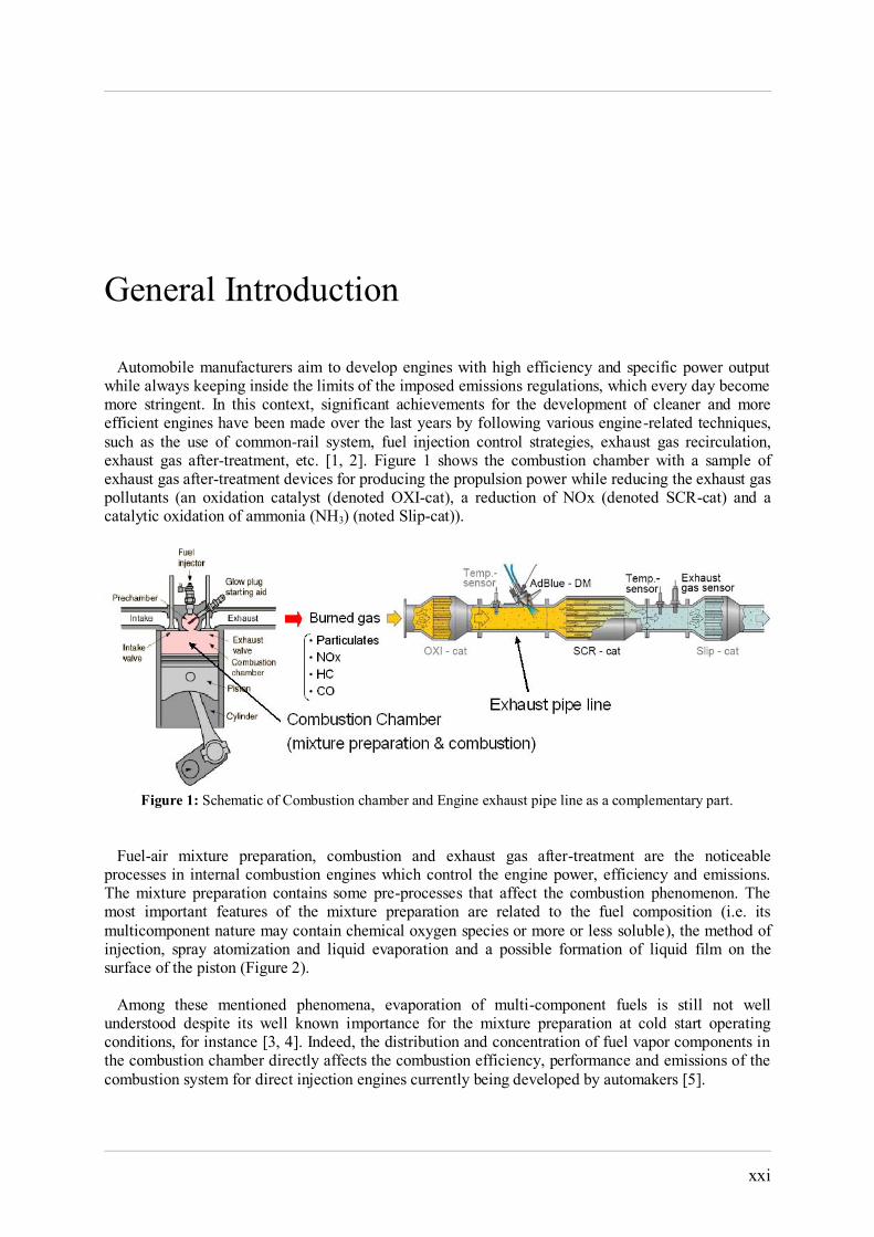
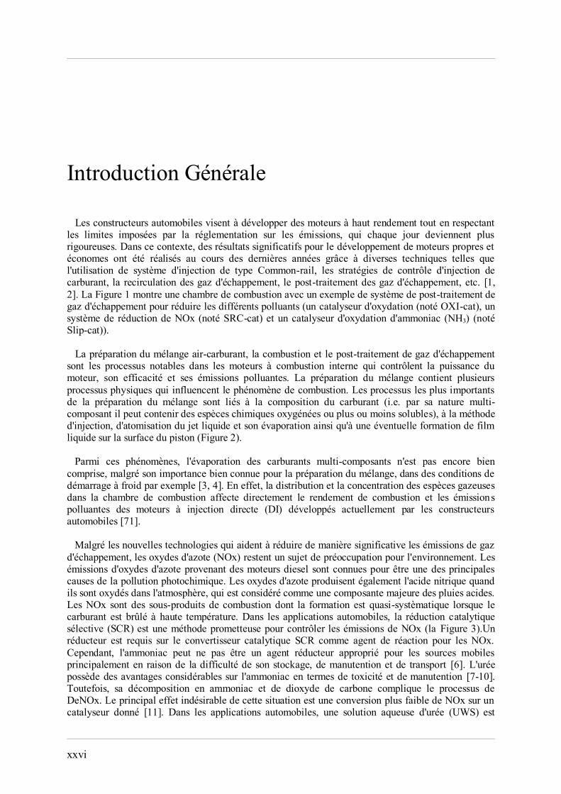
General Introduction Automobile manufacturers aim to develop engines with high efficiency and specific power output while always keeping inside the limits of the imposed emissions regulations, which every day become more stringent. In this context, significant achievements for the development of cleaner and more efficient engines have been made over the last years by following various engine-related techniques, such as the use of common-rail system, fuel injection control strategies, exhaust gas recirculation, exhaust gas after-treatment, etc. [1, 2]. Figure 1 shows the combustion chamber with a sample of exhaust gas after-treatment devices for producing the propulsion power while reducing the exhaust gas pollutants (an oxidation catalyst (denoted OXI-cat), a reduction of NOx (denoted SCR-cat) and a catalytic oxidation of ammonia (NH3) (noted Slip-cat)).
Figure 1: Schematic of Combustion chamber and Engine exhaust pipe line as a complementary part.
Fuel-air mixture preparation, combustion and exhaust gas after-treatment are the noticeable processes in internal combustion engines which control the engine power, efficiency and emissions. The mixture preparation contains some pre-processes that affect the combustion phenomenon. The most important features of the mixture preparation are related to the fuel composition (i.e. its multicomponent nature may contain chemical oxygen species or more or less soluble), the method of injection, spray atomization and liquid evaporation and a possible formation of liquid film on the surface of the piston (Figure 2). Among these mentioned phenomena, evaporation of multi-component fuels is still not well understood despite its well known importance for the mixture preparation at cold start operating conditions, for instance [3, 4]. Indeed, the distribution and concentration of fuel vapor components in the combustion chamber directly affects the combustion efficiency, performance and emissions of the combustion system for direct injection engines currently being developed by automakers [5].
xxii
Despite new technologies that significantly aid in reducing engine-out exhaust emissions, NOx (nitrogen oxides) is still the subject of environmental concern. Emissions of nitrogen oxides from the exhaust pipe of Diesel engines are known to be a major cause of photochemical air pollution. Nitrogen oxides also produce nitric acid when oxidized in the atmosphere, which is considered a major component of acid rain. Among the unwanted products, NOx play an important role in science and industry since their formation is inevitable when fuel is burnt at high temperature in a combustion process. In automotive applications, the urea-water-solution (UWS) based selective catalytic reduction (SCR) is a promising method to control NOx emissions (Figure 3). Ammonia is required on the SCR catalytic converter as a reaction agent for NOx. However, ammonia might not be a suitable reducing agent for mobile sources mainly due to the difficulties in its storage, handling and transportation [6]. Urea possesses considerable advantages over ammonia in terms of toxicity and handling [7-10]. However, its necessary decomposition into ammonia and carbon dioxide complicates the DeNOx process. The major undesirable effect of this is a lower NOx conversion on a given catalyst [11]. In mobile industries, UWS is used instead of ammonia and is injected into the exhaust pipe line to produce ammonia by thermolysis of urea and hydrolysis of iso-cyanic acid. Currently, most developed techniques use Urea-water-solution (UWS) containing 32.5 wt% urea by weight (trade name: AdBlue). This two-components mixture is sprayed into the exhaust gas (see Figure 1). The reducing agent (ammonia, NH3) is generated by evaporation of water, thermolysis of urea and hydrolysis of iso-cyanic acid (HNCO) [12]. In this process, the evaporation of water is influenced by the presence of the dissolved urea [13, 14]. The resulting spatial distribution of the reducing agent NH3 upstream to the catalyst is a crucial factor for the conversion of NOx [15]. For the study of such system, several physical processes (mainly evaporation of water and thermal decomposition of urea) need to be modeled. The present thesis contains two main parts:
The first part proposes multi-component evaporation models for droplets and liquid films in order to improve mixture preparation simulations inside the combustion chamber of automotive engines (Diesel, Gasoline, etc.).
The second part proposes a set of models including the evaporation of the urea-water solution (for the spray droplets and the liquid films) and the thermolysis of urea in the exhaust pipe of automotive engines. The present work develops numerically the UWS-SCR technology, (as illustrated in Figure 1), in order to reduce the NOx emissions. A schematic of a SCR system is shown in Figure 3.
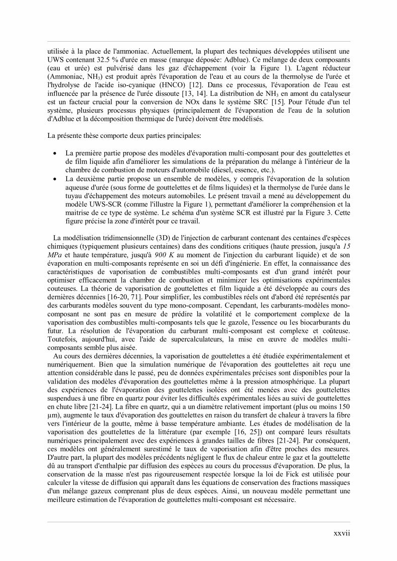
The three-dimensional modeling of injection of fuel containing hundreds of chemical components (until 300) into critical conditions (high pressures, until 15 MPa and high temperatures, until 900 K at the injection of liquid fuel) and its subsequent multi-component evaporation represents itself an engineering challenge. Knowing the vaporization characteristics of multi-component fuels is of great interest in order to efficiently optimize the combustion chamber and to avoid extensive experimental optimizations. The theory of single and/or multi component droplet vaporization has been developed during the past decades [5, 16-20]. Solving for multi-component fuel evaporation is complex and costly and for simplicity, real fuels have been represented by single-component fuel models (or surrogates). However, single-component fuel models are not able to predict the volatility and the complex behavior of the vaporization of multi-component fuels such as diesel, gasoline or future biofuels. Nowadays, with the aid of supercomputers, developing multi-component fuel models becomes more tractable. Droplet vaporization has intensively been investigated experimentally and numerically during the past decades. Although numerical simulation of droplet evaporation has received a considerable attention in the past, few experimental accurate data are available for the validation of droplet evaporation models even at atmospheric pressure. Most isolated droplet evaporation experiments have been conducted with the droplet suspended on a support fiber to avoid the experimental difficulties for free-falling droplets [21-24]. The support fiber which has a relatively large diameter (more or less 150 µm) increases the droplet evaporation rate due to the heat transfer through the fiber to the droplet even
xxiii
at low ambient temperatures. Droplet vaporization models from the literature (such as [16, 25]) have compared their numerical results mainly on the experiments with large sizes of fibers [21-24]. Consequently, these models have usually overestimated the vaporization rate. Moreover, most previous models neglect the heat flux between the gas and the droplet due to the enthalpy diffusion of species during the evaporation process. In addition, the mass conservation is not rigorously respected when Fick's law is used to model the diffusion velocity of more than two species in the mass fraction conservation equations of the gas mixture. Thus, a new model that could have a better estimation of multicomponent droplets evaporation is needed. While the idea of treating complex fuel mixtures and using continuous thermodynamics approach has recently been applied to practical engine fuel vaporization and combustion by Wang and Lee [26] and Lippert et al. [27], and needs less computation time [28], in the present study, discrete pure species approach have been adopted in order to be able to use kinetic schemes for combustion, auto-ignition and even for chemical reactions in the exhaust system (see Figure 1). Then, the first goal of the present work consists in the development of a multi-component droplets evaporation model based on a discrete species approach. This new model is going to be presented in the Chapter 1 of this manuscript.
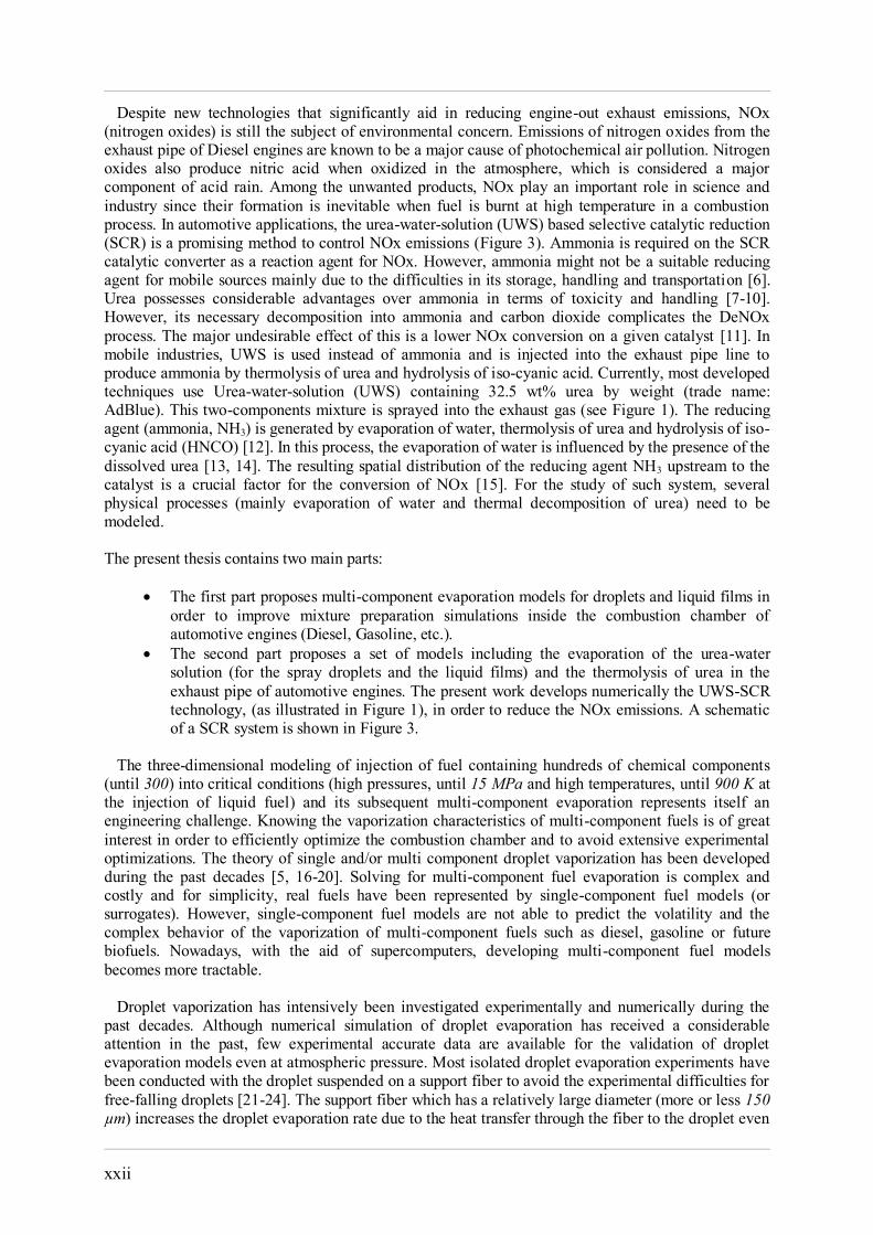
Figure 2: Principle phenomena (fuel injection, droplet and liquid film formation, evaporation and combustion)
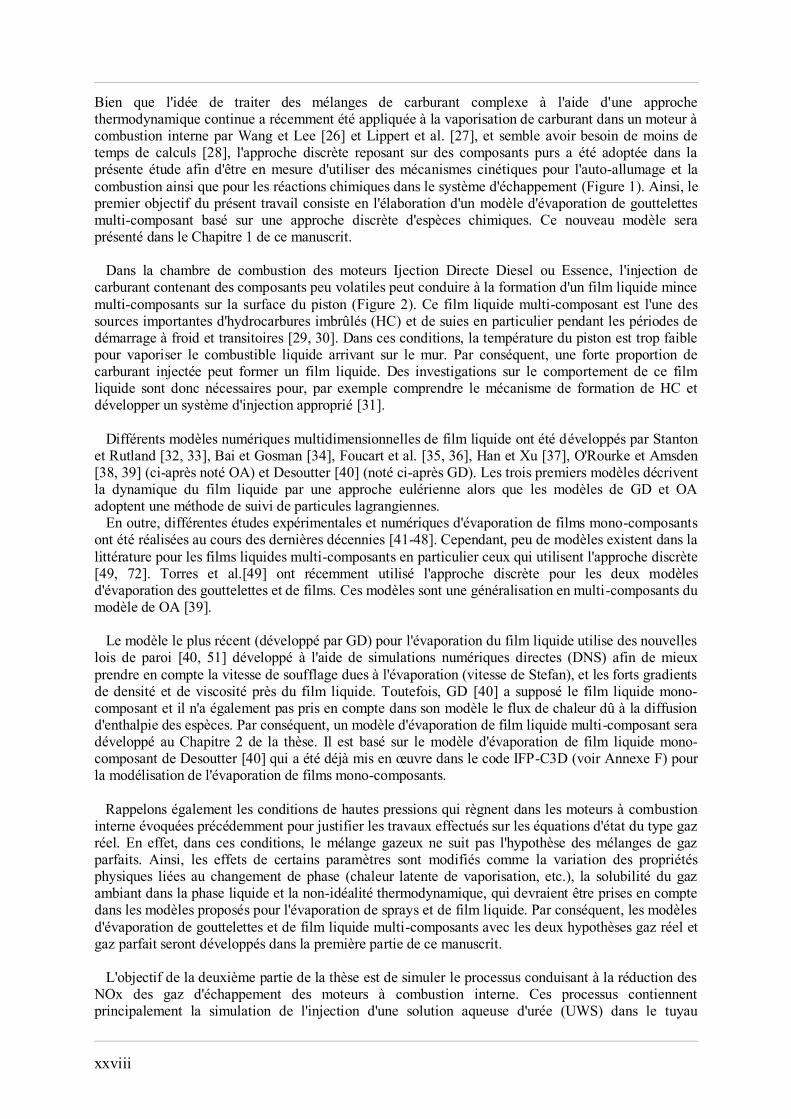
in a combustion chamber In the combustion chamber of diesel or gasoline engines, injection of fuel containing low volatile components may lead to the formation of a thin multi-component liquid film on the piston surface (Figure 2). This multi-component liquid film is one of the important sources of unburned hydrocarbon (HC) and soot especially during transient and cold start periods [29, 30]. In this condition, the temperature of the cylinder wall is too low to vaporize the liquid fuel impinged on the wall. Consequently, a high portion of injected fuel remains on the wall. Investigation of liquid fuel film behavior is important in order to understand the HC formation mechanism and to develop appropriate injection system [31]. Different multi-dimensional numerical models of liquid film have been developed by Stanton and Rutland [32, 33], Bai and Gosman [34], Foucart et al. [35, 36], Han and Xu [37], O'Rourke and Amsden [38, 39] (referred to subsequently as OA) and Desoutter [40] (referred to subsequently as GD). The first three models describe the dynamics of the liquid by an Eulerian approach whereas the models of GD and OA adopt a Lagrangian particle tracking method. In addition, some experimental and numerical single-component film evaporation studies have been performed [41-48] in the past few decades. However, few models exist in the literature for multi-component liquid films especially assuming the discrete approach [49, 50]. Torres et al. [49] used discrete approach for both spray and film evaporation models. These multi-component models are generalized from single-component evaporation model of OA [39]. The most recent model (developed by GD) for liquid film evaporation uses new wall functions [40, 51] developed using direct numerical simulations (DNS) in order to better take into account the blowing velocity due to evaporation (Stephan velocity), and the strong density and viscosity gradients
xxiv
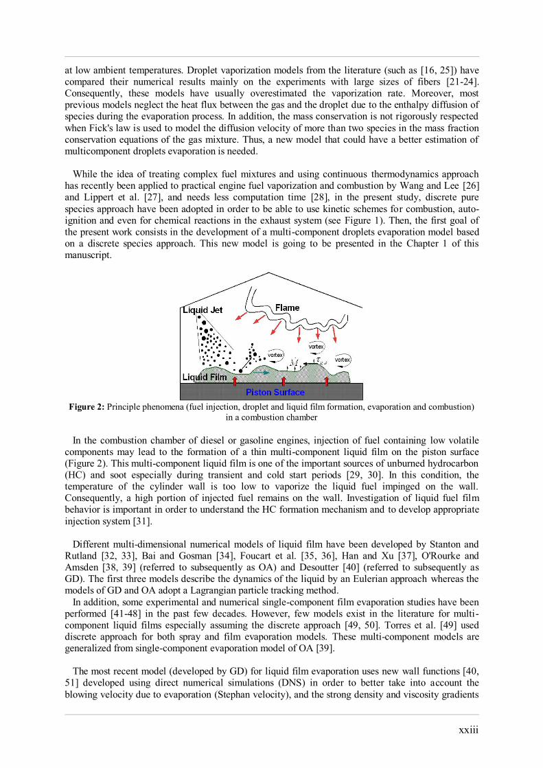
near the liquid film. However, GD [40] assumed the liquid film to be single-component and also the heat flux due to the enthalpy diffusion of species was not taken into account in his model. Consequently, a multi-component liquid film evaporation model will be developed in Chapter 2 of the thesis. It is based on Desoutter single-component film evaporation model [40] which was already implemented in IFP-C3D code (see Appendix E) for single-component film evaporation modeling. The conditions of high pressure prevailing in internal combustion engines may justify the use of a real gas equation of state (EOS). In fact, in this condition, gaseous fuel species do not follow the ideal mixture assumption. The influences of some parameters like the physical properties variation related to the phase change (like latent heat of vaporization, etc.), the ambient gas solubility in the liquid phase and the thermodynamic non-ideality should also be taken into account in the suggested droplet and film evaporation models. Therefore, multi-component droplets and liquid film evaporation models with both real and ideal mixture assumptions will be developed in the first part of this manuscript. The goal of the second part of the thesis is to simulate the processes leading to NOx reduction of engine exhaust gas. These processes contain mainly the simulation of the injection of an urea-water solution (UWS) to the exhaust pipe leading to the evaporation of water and the thermolysis of urea (see Figure 3). The evaporation of water and thermolysis of urea are the most significant processes for the production of ammonia. This ammonia will finally react with the exhaust gas (in the SCR system) to decrease the amount of NOx in the gas flowing to the atmosphere (as shown in Figure 3). Note that this latter process to reduce NOx in the SCR system is not part of the objectives of this study.
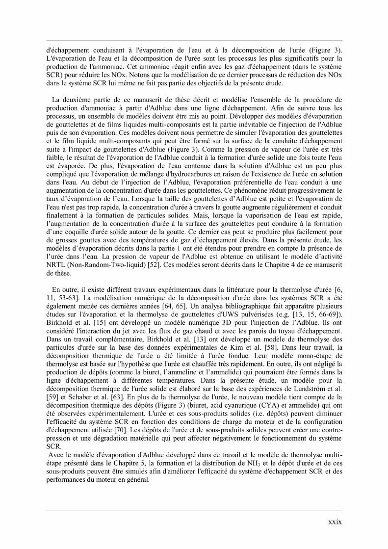
Figure 3: Schematic of a SCR system
The second part of this manuscript describes and models the entire process of production of ammonia from UWS in an exhaust pipe line. To monitor all processes, a set of models must be developed. In particular, multi-component droplet and liquid film evaporation models are crucial parts of the UWS injection and subsequent evaporation. These models should allow us to simulate the evaporation of multi-component droplets and liquid film that may be formed on the exhaust pipe surface due to the impact of UWS droplets (Figure 3). Since the vapor pressure of urea is very low, the result of the evaporation of the UWS is the production of solid urea once water is completely evaporated. Evaporation of water from UWS is a little more complicated than hydrocarbon mixture evaporation due to the presence of urea solute in the water. At the beginning of the injection of AdBlue, the preferential evaporation of water leads to an increase in urea concentration in the droplets. This phenomenon gradually reduces the rate of evaporation of water. When the UWS droplet size is small and the evaporation of water is slow, the concentration of urea throughout the droplet increases uniformly which finally leads to the formation of solid particle. But, when rapid water vaporization occurs on the droplet surface, urea concentration increases at the droplet surface which builds up a solid urea shell around the droplet. The last case occurs for larger droplets with higher heating rates. In this study, evaporation models described in Part I have been extended to take into account the presence of urea in water. The vapor pressure of the UWS will be obtained using NRTL (Non-Random Two-Liquids) activity model [52] which will be described in Chapter 4.
xxv
There are a number of experimental works in the literature for urea thermolysis [6, 11, 53-63]. Numerical modeling of urea thermolysis for SCR systems has been conducted since the past few years [64, 65]. Analyzing the literature, several studies on the evaporation and thermolysis of UWS from sprayed droplets can be found (e.g. [13, 15, 66-69]). Birkhold et al. [15] developed a 3D numerical computer model for injection of UWS. They considered the interaction of the spray with both the hot gas stream and walls of the exhaust pipe. In a complementary work [13] Birkhold et al. developed a thermolysis model for urea particles based on the experimental data of Kim et al. [58]. In their work, thermal decomposition of urea was limited to the molten urea. Their single-step thermolysis model is based on the assumption that urea is heated very quickly. In addition, they neglected the production of solid by-products (like biuret, ammeline and ammelide) which could be formed in the exhaust pipe for different temperature and/or gas flow conditions. In the present study, a model for thermal decomposition of solid urea is developed based on the experiments of Lundström et al. [59] and Schaber et al. [63]. In addition to the thermolysis of urea, the new model takes into account the thermal decomposition of solid by-products (shown in Figure 3) (like biuret, cyanuric acid-CYA and ammelide) which have been observed experimentally. Depending on engine loading conditions and exhaust configuration, urea and solid by-products deposits decrease the efficiency of the SCR system [70]. They may cause backpressure and material deteriorations and negatively affect the engine and SCR system operations and emission performances. With the developed evaporation of UWS and the multi-step thermolysis models presented in Chapter 5, the formation and distribution of NH3 and deposition of urea and its by-products can be simulated to improve SCR exhaust system efficiency and engine performance in general. The models developed in the present work are implemented in the IFP-C3D code (see Appendix E) and used to simulate the mixture preparation and combustion of different bio-fuels in a typical Diesel engine operating with conventional fuels and mixtures of first (including esters) and second (like ethanol) generation bio-fuel. The numerical results are discussed in Chapter 3. Also, the UWS injection, water evaporation and urea thermolysis have been simulated in a typical exhaust pipe configuration in Chapter 6. Finally, general conclusions are drawn in Chapter 7 along with future works indication.
xxvi
Introduction Générale Les constructeurs automobiles visent à développer des moteurs à haut rendement tout en respectant les limites imposées par la réglementation sur les émissions, qui chaque jour deviennent plus rigoureuses. Dans ce contexte, des résultats significatifs pour le développement de moteurs propres et économes ont été réalisés au cours des dernières années grâce à diverses techniques telles que l'utilisation de système d'injection de type Common-rail, les stratégies de contrôle d'injection de carburant, la recirculation des gaz d'échappement, le post-traitement des gaz d'échappement, etc. [1, 2]. La Figure 1 montre une chambre de combustion avec un exemple de système de post-traitement de gaz d'échappement pour réduire les différents polluants (un catalyseur d'oxydation (noté OXI-cat), un système de réduction de NOx (noté SRC-cat) et un catalyseur d'oxydation d'ammoniac (NH3) (noté Slip-cat)). La préparation du mélange air-carburant, la combustion et le post-traitement de gaz d'échappement sont les processus notables dans les moteurs à combustion interne qui contrôlent la puissance du moteur, son efficacité et ses émissions polluantes. La préparation du mélange contient plusieurs processus physiques qui influencent le phénomène de combustion. Les processus les plus importants de la préparation du mélange sont liés à la composition du carburant (i.e. par sa nature multi-composant il peut contenir des espèces chimiques oxygénées ou plus ou moins solubles), à la méthode d'injection, d'atomisation du jet liquide et son évaporation ainsi qu'à une éventuelle formation de film liquide sur la surface du piston (Figure 2). Parmi ces phénomènes, l'évaporation des carburants multi-composants n'est pas encore bien comprise, malgré son importance bien connue pour la préparation du mélange, dans des conditions de démarrage à froid par exemple [3, 4]. En effet, la distribution et la concentration des espèces gazeuses dans la chambre de combustion affecte directement le rendement de combustion et les émissions polluantes des moteurs à injection directe (DI) développés actuellement par les constructeurs automobiles [71]. Malgré les nouvelles technologies qui aident à réduire de manière significative les émissions de gaz d'échappement, les oxydes d'azote (NOx) restent un sujet de préoccupation pour l'environnement. Les émissions d'oxydes d'azote provenant des moteurs diesel sont connues pour être une des principales causes de la pollution photochimique. Les oxydes d'azote produisent également l'acide nitrique quand ils sont oxydés dans l'atmosphère, qui est considéré comme une composante majeure des pluies acides. Les NOx sont des sous-produits de combustion dont la formation est quasi-systèmatique lorsque le carburant est brûlé à haute température. Dans les applications automobiles, la réduction catalytique sélective (SCR) est une méthode prometteuse pour contrôler les émissions de NOx (la Figure 3).Un réducteur est requis sur le convertisseur catalytique SCR comme agent de réaction pour les NOx. Cependant, l'ammoniac peut ne pas être un agent réducteur approprié pour les sources mobiles principalement en raison de la difficulté de son stockage, de manutention et de transport [6]. L'urée possède des avantages considérables sur l'ammoniac en termes de toxicité et de manutention [7-10]. Toutefois, sa décomposition en ammoniac et de dioxyde de carbone complique le processus de DeNOx. Le principal effet indésirable de cette situation est une conversion plus faible de NOx sur un catalyseur donné [11]. Dans les applications automobiles, une solution aqueuse d'urée (UWS) est
xxvii
utilisée à la place de l'ammoniac. Actuellement, la plupart des techniques développées utilisent une UWS contenant 32.5 % d'urée en masse (marque déposée: Adblue). Ce mélange de deux composants (eau et urée) est pulvérisé dans les gaz d'échappement (voir la Figure 1). L'agent réducteur (Ammoniac, NH3) est produit après l'évaporation de l'eau et au cours de la thermolyse de l'urée et l'hydrolyse de l'acide iso-cyanique (HNCO) [12]. Dans ce processus, l'évaporation de l'eau est influencée par la présence de l'urée dissoute [13, 14]. La distribution de NH3 en amont du catalyseur est un facteur crucial pour la conversion de NOx dans le système SRC [15]. Pour l'étude d'un tel système, plusieurs processus physiques (principalement de l'évaporation de l'eau de la solution d'Adblue et la décomposition thermique de l'urée) doivent être modélisés. La présente thèse comporte deux parties principales: La première partie propose des modèles d'évaporation multi-composant pour des gouttelettes et
de film liquide afin d'améliorer les simulations de la préparation du mélange à l'intérieur de la chambre de combustion de moteurs d'automobile (diesel, essence, etc.).
La deuxième partie propose un ensemble de modèles, y compris l'évaporation de la solution aqueuse d'urée (sous forme de gouttelettes et de films liquides) et la thermolyse de l'urée dans le tuyau d'échappement des moteurs automobiles. Le présent travail a mené au développement du modèle UWS-SCR (comme l'illustre la Figure 1), permettant d'améliorer la compréhension et la maitrise de ce type de système. Le schéma d'un système SCR est illustré par la Figure 3. Cette figure précise la zone d'intérêt pour ce travail.
La modélisation tridimensionnelle (3D) de l'injection de carburant contenant des centaines d'espèces chimiques (typiquement plusieurs centaines) dans des conditions critiques (haute pression, jusqu'a 15 MPa et haute température, jusqu'à 900 K au moment de l'injection du carburant liquide) et de son évaporation en multi-composants représente en soi un défi d'ingénierie. En effet, la connaissance des caractéristiques de vaporisation de combustibles multi-composants est d'un grand intérêt pour optimiser efficacement la chambre de combustion et minimizer les optimisations expérimentales couteuses. La théorie de vaporisation de gouttelettes et film liquide a été développée au cours des dernières décennies [16-20, 71]. Pour simplifier, les combustibles réels ont d'abord été représentés par des carburants modèles souvent du type mono-composant. Cependant, les carburants-modèles mono-composant ne sont pas en mesure de prédire la volatilité et le comportement complexe de la vaporisation des combustibles multi-composants tels que le gazole, l'essence ou les biocarburants du futur. La résolution de l'évaporation du carburant multi-composant est complexe et coûteuse. Toutefois, aujourd'hui, avec l'aide de supercalculateurs, la mise en œuvre de modèles multi-composants semble plus aisée. Au cours des dernières décennies, la vaporisation de gouttelettes a été étudiée expérimentalement et numériquement. Bien que la simulation numérique de l'évaporation des gouttelettes ait reçu une attention considérable dans le passé, peu de données expérimentales précises sont disponibles pour la validation des modèles d'évaporation des gouttelettes même à la pression atmosphérique. La plupart des expériences de l'évaporation des gouttelettes isolées ont été menées avec des gouttelettes suspendues à une fibre en quartz pour éviter les difficultés expérimentales liées au suivi de gouttelettes en chute libre [21-24]. La fibre en quartz, qui a un diamètre relativement important (plus ou moins 150 µm), augmente le taux d'évaporation des gouttelettes en raison du transfert de chaleur à travers la fibre vers l'intérieur de la goutte, même à basse température ambiante. Les études de modélisation de la vaporisation des gouttelettes de la littérature (par exemple [16, 25]) ont comparé leurs résultats numériques principalement avec des expériences à grandes tailles de fibres [21-24]. Par conséquent, ces modèles ont généralement surestimé le taux de vaporisation afin d'être proches des mesures. D'autre part, la plupart des modèles précédents négligent le flux de chaleur entre le gaz et la gouttelette dû au transport d'enthalpie par diffusion des espèces au cours du processus d'évaporation. De plus, la conservation de la masse n'est pas rigoureusement respectée lorsque la loi de Fick est utilisée pour calculer la vitesse de diffusion qui apparaît dans les équations de conservation des fractions massiques d'un mélange gazeux comprenant plus de deux espèces. Ainsi, un nouveau modèle permettant une meilleure estimation de l'évaporation de gouttelettes multi-composant est nécessaire.
xxviii
Bien que l'idée de traiter des mélanges de carburant complexe à l'aide d'une approche thermodynamique continue a récemment été appliquée à la vaporisation de carburant dans un moteur à combustion interne par Wang et Lee [26] et Lippert et al. [27], et semble avoir besoin de moins de temps de calculs [28], l'approche discrète reposant sur des composants purs a été adoptée dans la présente étude afin d'être en mesure d'utiliser des mécanismes cinétiques pour l'auto-allumage et la combustion ainsi que pour les réactions chimiques dans le système d'échappement (Figure 1). Ainsi, le premier objectif du présent travail consiste en l'élaboration d'un modèle d'évaporation de gouttelettes multi-composant basé sur une approche discrète d'espèces chimiques. Ce nouveau modèle sera présenté dans le Chapitre 1 de ce manuscrit. Dans la chambre de combustion des moteurs Ijection Directe Diesel ou Essence, l'injection de carburant contenant des composants peu volatiles peut conduire à la formation d'un film liquide mince multi-composants sur la surface du piston (Figure 2). Ce film liquide multi-composant est l'une des sources importantes d'hydrocarbures imbrûlés (HC) et de suies en particulier pendant les périodes de démarrage à froid et transitoires [29, 30]. Dans ces conditions, la température du piston est trop faible pour vaporiser le combustible liquide arrivant sur le mur. Par conséquent, une forte proportion de carburant injectée peut former un film liquide. Des investigations sur le comportement de ce film liquide sont donc nécessaires pour, par exemple comprendre le mécanisme de formation de HC et développer un système d'injection approprié [31]. Différents modèles numériques multidimensionnelles de film liquide ont été développés par Stanton et Rutland [32, 33], Bai et Gosman [34], Foucart et al. [35, 36], Han et Xu [37], O'Rourke et Amsden [38, 39] (ci-après noté OA) et Desoutter [40] (noté ci-après GD). Les trois premiers modèles décrivent la dynamique du film liquide par une approche eulérienne alors que les modèles de GD et OA adoptent une méthode de suivi de particules lagrangiennes. En outre, différentes études expérimentales et numériques d'évaporation de films mono-composants ont été réalisées au cours des dernières décennies [41-48]. Cependant, peu de modèles existent dans la littérature pour les films liquides multi-composants en particulier ceux qui utilisent l'approche discrète [49, 72]. Torres et al.[49] ont récemment utilisé l'approche discrète pour les deux modèles d'évaporation des gouttelettes et de films. Ces modèles sont une généralisation en multi-composants du modèle de OA [39]. Le modèle le plus récent (développé par GD) pour l'évaporation du film liquide utilise des nouvelles lois de paroi [40, 51] développé à l'aide de simulations numériques directes (DNS) afin de mieux prendre en compte la vitesse de soufflage dues à l'évaporation (vitesse de Stefan), et les forts gradients de densité et de viscosité près du film liquide. Toutefois, GD [40] a supposé le film liquide mono-composant et il n'a également pas pris en compte dans son modèle le flux de chaleur dû à la diffusion d'enthalpie des espèces. Par conséquent, un modèle d'évaporation de film liquide multi-composant sera développé au Chapitre 2 de la thèse. Il est basé sur le modèle d'évaporation de film liquide mono-composant de Desoutter [40] qui a été déjà mis en œuvre dans le code IFP-C3D (voir Annexe F) pour la modélisation de l'évaporation de films mono-composants. Rappelons également les conditions de hautes pressions qui règnent dans les moteurs à combustion interne évoquées précédemment pour justifier les travaux effectués sur les équations d'état du type gaz réel. En effet, dans ces conditions, le mélange gazeux ne suit pas l'hypothèse des mélanges de gaz parfaits. Ainsi, les effets de certains paramètres sont modifiés comme la variation des propriétés physiques liées au changement de phase (chaleur latente de vaporisation, etc.), la solubilité du gaz ambiant dans la phase liquide et la non-idéalité thermodynamique, qui devraient être prises en compte dans les modèles proposés pour l'évaporation de sprays et de film liquide. Par conséquent, les modèles d'évaporation de gouttelettes et de film liquide multi-composants avec les deux hypothèses gaz réel et gaz parfait seront développés dans la première partie de ce manuscrit. L'objectif de la deuxième partie de la thèse est de simuler le processus conduisant à la réduction des NOx des gaz d'échappement des moteurs à combustion interne. Ces processus contiennent principalement la simulation de l'injection d'une solution aqueuse d'urée (UWS) dans le tuyau
xxix
d'échappement conduisant à l'évaporation de l'eau et à la décomposition de l'urée (Figure 3). L'évaporation de l'eau et la décomposition de l'urée sont les processus les plus significatifs pour la production de l'ammoniac. Cet ammoniac réagit enfin avec les gaz d'échappement (dans le système SCR) pour réduire les NOx. Notons que la modélisation de ce dernier processus de réduction des NOx dans le système SCR lui même ne fait pas partie des objectifs de la présente étude. La deuxième partie de ce manuscrit de thèse décrit et modélise l'ensemble de la procédure de production d'ammoniac à partir d'Adblue dans une ligne d'échappement. Afin de suivre tous les processus, un ensemble de modèles doivent être mis au point. Développer des modèles d'évaporation de gouttelettes et de films liquides multi-composants est la partie inévitable de l'injection de l'Adblue puis de son évaporation. Ces modèles doivent nous permettre de simuler l'évaporation des gouttelettes et le film liquide multi-composants qui peut être formé sur la surface de la conduite d'échappement suite à l'impact de gouttelettes d'Adblue (Figure 3). Comme la pression de vapeur de l'urée est très faible, le résultat de l'évaporation de l'Adblue conduit à la formation d'urée solide une fois toute l'eau est évaporée. De plus, l'évaporation de l'eau contenue dans la solution d'Adblue est un peu plus compliqué que l'évaporation de mélange d'hydrocarbures en raison de l'existence de l'urée en solution dans l'eau. Au début de l’injection de l’Adblue, l'évaporation préférentielle de l'eau conduit à une augmentation de la concentration d'urée dans les gouttelettes. Ce phénomène réduit progressivement le taux d’évaporation de l’eau. Lorsque la taille des gouttelettes d’Adblue est petite et l'évaporation de l'eau n'est pas trop rapide, la concentration d'urée à travers la goutte augmente régulièrement et conduit finalement à la formation de particules solides. Mais, lorsque la vaporisation de l'eau est rapide, l’augmentation de la concentration d'urée à la surface des gouttelettes peut conduire à la formation d’une coquille d'urée solide autour de la goutte. Ce dernier cas peut se produire plus facilement pour de grosses gouttes avec des températures de gaz d’échappement élevés. Dans la présente étude, les modèles d’évaporation décrits dans la partie 1 ont été étendus pour prendre en compte la présence de l’urée dans l’eau. La pression de vapeur de l'Adblue est obtenue en utilisant le modèle d’activité NRTL (Non-Random-Two-liquid) [52]. Ces modèles seront décrits dans le Chapitre 4 de ce manuscrit de thèse. En outre, il existe différent travaux expérimentaux dans la littérature pour la thermolyse d'urée [6, 11, 53-63]. La modélisation numérique de la décomposition d'urée dans les systèmes SCR a été également menée ces dernières années [64, 65]. Un analyse bibliographique fait apparaître plusieurs études sur l'évaporation et la thermolyse de gouttelettes d'UWS pulvérisées (e.g. [13, 15, 66-69]). Birkhold et al. [15] ont développé un modèle numérique 3D pour l'injection de l’Adblue. Ils ont considéré l'interaction du jet avec les flux de gaz chaud et avec les parois du tuyau d'échappement. Dans un travail complémentaire, Birkhold et al. [13] ont développé un modèle de thermolyse des particules d'urée sur la base des données expérimentales de Kim et al. [58]. Dans leur travail, la décomposition thermique de l'urée a été limitée à l'urée fondue. Leur modèle mono-étape de thermolyse est basée sur l'hypothèse que l'urée est chauffée très rapidement. En outre, ils ont négligé la production de dépôts (comme la biuret, l’ammeline et l’ammelide) qui pourraîent être formés dans la ligne d'échappement à différentes températures. Dans la présente étude, un modèle pour la décomposition thermique de l'urée solide est élaboré sur la base des expériences de Lundström et al. [59] et Schaber et al. [63]. En plus de la thermolyse de l'urée, le nouveau modèle tient compte de la décomposition thermique des dépôts (Figure 3) (biuret, acid cyanurique (CYA) et ammelide) qui ont été observées expérimentalement. L'urée et ces sous-produits solides (i.e. dépôts) peuvent diminuer l'efficacité du système SCR en fonction des conditions de charge du moteur et de la configuration d'échappement utilisée [70]. Les dépôts de l'urée et de sous-produits solides peuvent créer une contre-pression et une dégradation matérielle qui peut affecter négativement le fonctionnement du système SCR. Avec le modèle d'évaporation d'Adblue développé dans ce travail et le modèle de thermolyse multi-étape présenté dans le Chapitre 5, la formation et la distribution de NH3 et le dépôt d'urée et de ces sous-produits peuvent être simulés afin d'améliorer l'efficacité du système d'échappement SCR et des performances du moteur en général.
xxx
Les modèles développés dans le présent travail sont mis en œuvre dans le code industriel IFP-C3D et utilisés pour simuler la préparation du mélange et la combustion de différents biocarburants dans un moteur diesel fonctionnant avec des fuels classiques ainsi que des mélanges de bio-carburants de première (incluant des Esters) et seconde génération (comme l’éthanol). Les résultats numériques sont discutés dans le Chapitre 3. Le Chapitre 6 présente les résultats numériques obtenus dans une configuration d'échappement typique en utilisant les différents modèles d'injection d'Adblue, d'évaporation et de thermolyse d'urée. Enfin, les conclusions générales ainsi les perspectives de cette thèse sont résumées dans le Chapitre 7.
xxxi
Part I
Multi-component Evaporation modeling
xxxii
Introduction The first part of the thesis is dedicated to the development and validation of a multi-component droplet model and a multi-component liquid film evaporation model. It contains three chapters: In the first chapter, a new multi-component droplet evaporation model is presented. Similar to the classical models, the new droplet evaporation model uses Navier-Stokes equations for mass, momentum and energy conservation. The main features of the new multi-component droplet evaporation model are: introducing an expression of the Stephan velocity to ensure gas mass conservation and taking into account the heat flux due to the species diffusion between the gas and liquid droplets. The multi-component droplet evaporation model with real and ideal mixture hypotheses is then implemented in the IFP-C3D code and validated against the most recent experimental data of Chauveau et al. [73] for single-component isolated droplet. Some multi-component evaporation simulations are also provided and the results are discussed. The second chapter of the thesis proposes a multi-component liquid film evaporation model with discrete approach. This model is based on the single-component liquid film evaporation model of G. Desoutter [40]. Liquid film evaporation model resolves Navier-Stokes equations for liquid and gas phases which have been already used for droplet vaporization modeling. The evaporation of droplet or liquid film consists of resolving two phase flow equations as well as satisfying the thermodynamic equilibrium condition at the liquid-gas interface. Single-component mass fraction, dynamic and thermal wall laws developed by Desoutter et al. [51] are also generalized for the multi-component model which is described in detail in Appendix D The present film evaporation model is implemented into the multi-dimensional IFP-C3D code and applied to calculate evaporation processes of single and multi-component fuel film. Differences between representing model fuels using the single and multi-component fuel descriptions are discussed. The model is also used to simulate the film formation and evaporation of single iso-octane fuel which has been investigated experimentally by Ref. [74]. In the third chapter, both droplet and liquid film evaporation models implemented in the IFP-C3D code are used to simulate the mixture preparation in a typical internal combustion engine. The numerical results of the models allow us to assess the contribution of the developments made during this work in the context of industrial applications.
Chapter 1
Multi-component droplet evaporation 1.1 Introduction Droplet vaporization has intensively been investigated experimentally and numerically during the past decades. Indeed, this phenomenon is of interest to many fields of engineering applications. The detailed evaporation of multi-component droplets during the combustion of fuel sprays in automotive engines or gas turbines is a prominent example. The influence of the volatility between the numerous components of real fuels on pollutant emissions still needs to be understood. Some worthy studies have been performed on the multi-component droplet evaporation [18-20, 75-79]. The modeling of multi-component fuels began with Landis and Mills [80] who studied the evaporation of heptane-octane droplet, followed by studies by Sirignano and Law [81] and Law [82]. Multi-component droplet evaporation modeling is classified into two types, i.e., discrete multi-component model and continuous thermodynamic model. Discrete methods describe the multi-component nature of practical engine fuels and use specific species (typically 2-15 components) to represent real fuels. In this method, (used for the evaporation of multi-component droplets [18, 49, 83, 84]) the species concentration equation is solved for each component and the individual droplet (or generally liquid) components are tracked during the evaporation process. Although this method gives satisfying results for droplet evaporation, the cost of computation due to the solution of additional transport equations for liquids with large number of components limits this approach to liquids containing few components. The second method is the so-called continuous multi-component fuel model. It has recently been used for multi-component droplet evaporation [17, 20, 75, 85]. The composition of the fuel liquid and vapor, and consequently the system properties, are represented and described by a continuous probability density function (PDF). This method has first been developed by Cotterman et al. [86] for chemical field. Tamim and Hallett [20] then presented a model for the evaporation of droplets of multi-component liquids in which the mixture composition, properties and vapor-liquid equilibrium are described by the method of continuous thermodynamics using a Gamma-PDF for the species molecular weight. In this model, transport equations for the parameters (i.e. the two first moments) of the distribution function describing the mixture composition are derived and solved numerically. Although the continuous thermodynamic model for multi-component droplets evaporation seems to consume less computation time than the discrete method, its accuracy may depend on the assumed PDF choice. In addition, all the physical properties of the fuel need to be related to the molecular weight which is not always possible.
Chapter 1 Multi-component droplet evaporation
2
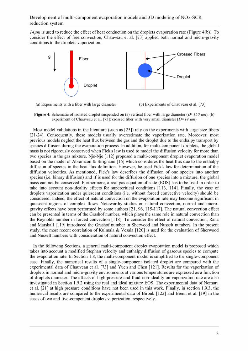
The multi-component droplet vaporization in internal combustion engines usually occurs at high pressure and temperature conditions. When fuel is injected at a higher temperature than its saturation temperature, the fuel is superheated and it is under supercritical condition (i.e., it is at a pressure or temperature exceeding its critical value [87, 88].). The supercritical droplet vaporization has been the subject of many theoretical and experimental investigations [21, 25, 89-96]. Scientists agree on the fact that under high pressure conditions, the vaporization process has many important aspects that are not adequately considered by low pressure models. As an example, the gas phase non-ideality and liquid phase solubility of gases can not be neglected for the high pressure condition. The effect of supercritical conditions on the vapor-liquid equilibrium and droplet lifetime should also be taken into account in the droplet evaporation modeling using an appropriate equation of state (EOS). In high pressure conditions, the liquid and gas phase thermo-physical properties become pressure dependent. At pressures near or above the critical pressure, the latent heat of vaporization reduces to zero and the densities of liquid and gas become equal at the droplet surface. In the above conditions, transient effects in the gas phase become as important as those in the liquid phase, since the characteristic times for transport processes in the two phases become comparable [90]. High pressure and temperature conditions may then lead to gas phase unsteadiness during the droplet vaporization process. The gas phase quasi-steadiness assumption, based on the argument that the gas-phase transport rate is much faster than the rate at which the properties at droplet surface change due to the significant disparity between the gas and liquid densities and valid only for low pressure conditions [82, 91, 97], underestimates the vaporization rate of droplets [98]. In situations where the droplets have a relative translational velocity with respect to the surrounding gaseous medium [99], the gas flow around the droplet which leads to the shear interaction of the two phases, establishes droplet internal motion. This behavior has been studied and used for droplet evaporation modeling in the literature [16, 82, 100-102]. It is shown that the droplet internal circulation increases both heat and mass transport, which affect the evaporation process [99]. However, the effect of internal circulation on the rate of mass transport for small droplets may not be significant. Indeed, conduction heat transfer inside small droplets can be neglected. In this case, the droplet thermal conductivity is assumed to be infinite and the temperature inside the droplet is spatially uniform and is equal to its surface temperature (i.e., infinite thermal conductivity hypothesis). However, this is not true for big droplets as shown by measurements of the temperature distribution inside each droplets [103, 104]. Some works take into account the droplet finite thermal conductivity [102, 105, 106], in which the heat is transferred within the liquid by thermal conduction. In some recent works the finite thermal conduction model is generalized to take into account the internal circulation inside droplets [102, 107] using the Peclet number. This approach is called "effective thermal conduction model". The same behavior is observed for the species diffusion in liquid phase. In the case of multi-component droplets evaporation, different components evaporate at different rates, creating concentration gradients in the liquid phase which lead to liquid phase mass diffusion. This effect has been studied in the literature [80, 107-109] with a definition similar to the finite or effective thermal conduction (i.e., finite or effective diffusion). However, for multi-component droplets with close volatilities of components, this hypothesis can be simplified in to the infinite diffusion assumption. Although numerical simulation of the mentioned phenomena has received a considerable attention in the past, few accurate experimental data are available for validation even at atmospheric pressure. Most isolated droplet evaporation experiments have been conducted with the droplet suspended on a support fiber [21-24] to avoid the experimental difficulties of free-falling droplets [110]. The support fiber (as can be seen in Figure 4(a)) has a relatively large diameter (approximately 150 µm) and increases the droplet evaporation rate due to the heat transfer through the fiber to the droplet even at low ambient temperatures. Yang & Wong [111] have studied the effects of heat conduction into the droplets through the fiber and the liquid-phase absorption of the radiation from the furnace wall on the evaporation rate of droplets at micro-gravity condition. They found that without considering these effects, there is a large discrepancy between their theoretical results and the experimental data of Nomura et al. [21]. More recently, Chauveau et al. [73] studied the effects of fiber diameter and gas temperature on droplet vaporization. In their experiments, a cross micro-fiber with small diameter of
Development of multi-component evaporation models and 3D modeling of NOx-SCR reduction system
3
14µm is used to reduce the effect of heat conduction on the droplets evaporation rate (Figure 4(b)). To consider the effect of free convection, Chauveau et al. [73] applied both normal and micro-gravity conditions to the droplets vaporization.
(a) Experiments with a fiber with large diameter
(b) Experiments of Chauveau et al. [73]
Figure 4: Schematic of isolated droplet suspended on (a) vertical fiber with large diameter (D≈150 µm), (b) experiment of Chauveau et al. [73]: crossed fiber with very small diameter (D=14 µm)
Most model validations in the literature (such as [25]) rely on the experiments with large size fibers [21-24]. Consequently, these models usually overestimate the vaporization rate. Moreover, most previous models neglect the heat flux between the gas and the droplet due to the enthalpy transport by species diffusion during the evaporation process. In addition, for multi-component droplets, the global mass is not rigorously conserved when Fick's law is used to model the diffusion velocity for more than two species in the gas mixture. Nje-Nje [112] proposed a multi-component droplet evaporation model based on the model of Abramzon & Sirignano [16] which consideres the heat flux due to the enthalpy diffusion of species in the heat flux definition. However, he used Fick's law for determination of the diffusion velocities. As mentioned, Fick's law describes the diffusion of one species into another species (i.e. binary diffusion) and if is used for the diffusion of one species into a mixture, the global mass can not be conserved. Furthermore, a real gas equation of state (EOS) has to be used in order to take into account non-ideality effects for supercritical conditions [113, 114]. Finally, the case of droplets vaporization under quiescent conditions (i.e. without forced convective velocity) should be considered. Indeed, the effect of natural convection on the evaporation rate may become significant in quiescent regions of complex flows. Noteworthy studies on natural convection, normal and micro-gravity effects have been performed by some authors [21, 96, 115-117]. The natural convection effect can be presented in terms of the Grashof number, which plays the same role in natural convection than the Reynolds number in forced convection [118]. To consider the effect of natural convection, Ranz and Marshall [119] introduced the Grashof number in Sherwood and Nusselt numbers. In the present study, the most recent correlation of Kulmala & Vesala [120] is used for the evaluation of Sherwood and Nusselt numbers with consideration of natural convection effect. In the following Sections, a general multi-component droplet evaporation model is proposed which takes into account a modified Stephan velocity and enthalpy diffusion of gaseous species to compute the evaporation rate. In Section 1.8, the multi-component model is simplified to the single-component case. Finally, the numerical results of a single-component isolated droplet are compared with the experimental data of Chauveau et al. [73] and Yuen and Chen [121]. Results for the vaporization of droplets in normal and micro-gravity environments at various temperatures are expressed as a function of droplets diameter. The effects of high pressure and fluid non-ideality on vaporization rate are also investigated in Section 1.9.2 using the real and ideal mixture EOS. The experimental data of Nomura et al. [21] at high pressure conditions have not been used in this work. Finally, in section 1.9.3, the numerical results are compared to the experimental data of Birouk [122] and Brenn et al. [19] in the cases of two and five-component droplets vaporization, respectively.
Fiber
Droplet
g
Droplet
Crossed Fibers
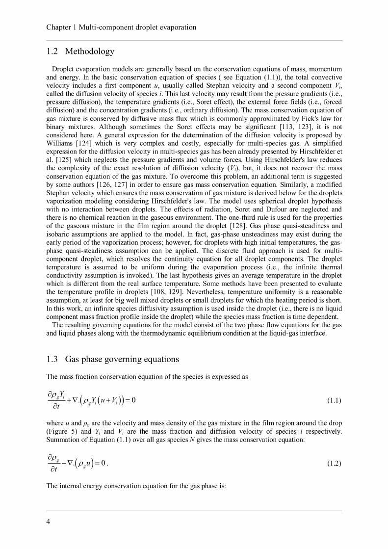
Chapter 1 Multi-component droplet evaporation
4
1.2 Methodology Droplet evaporation models are generally based on the conservation equations of mass, momentum and energy. In the basic conservation equation of species ( see Equation (1.1)), the total convective velocity includes a first component u, usually called Stephan velocity and a second component Vi, called the diffusion velocity of species i. This last velocity may result from the pressure gradients (i.e., pressure diffusion), the temperature gradients (i.e., Soret effect), the external force fields (i.e., forced diffusion) and the concentration gradients (i.e., ordinary diffusion). The mass conservation equation of gas mixture is conserved by diffusive mass flux which is commonly approximated by Fick's law for binary mixtures. Although sometimes the Soret effects may be significant [113, 123], it is not considered here. A general expression for the determination of the diffusion velocity is proposed by Williams [124] which is very complex and costly, especially for multi-species gas. A simplified expression for the diffusion velocity in multi-species gas has been already presented by Hirschfelder et al. [125] which neglects the pressure gradients and volume forces. Using Hirschfelder's law reduces the complexity of the exact resolution of diffusion velocity (Vi), but, it does not recover the mass conservation equation of the gas mixture. To overcome this problem, an additional term is suggested by some authors [126, 127] in order to ensure gas mass conservation equation. Similarly, a modified Stephan velocity which ensures the mass conservation of gas mixture is derived below for the droplets vaporization modeling considering Hirschfelder's law. The model uses spherical droplet hypothesis with no interaction between droplets. The effects of radiation, Soret and Dufour are neglected and there is no chemical reaction in the gaseous environment. The one-third rule is used for the properties of the gaseous mixture in the film region around the droplet [128]. Gas phase quasi-steadiness and isobaric assumptions are applied to the model. In fact, gas-phase unsteadiness may exist during the early period of the vaporization process; however, for droplets with high initial temperatures, the gas-phase quasi-steadiness assumption can be applied. The discrete fluid approach is used for multi-component droplet, which resolves the continuity equation for all droplet components. The droplet temperature is assumed to be uniform during the evaporation process (i.e., the infinite thermal conductivity assumption is invoked). The last hypothesis gives an average temperature in the droplet which is different from the real surface temperature. Some methods have been presented to evaluate the temperature profile in droplets [108, 129]. Nevertheless, temperature uniformity is a reasonable assumption, at least for big well mixed droplets or small droplets for which the heating period is short. In this work, an infinite species diffusivity assumption is used inside the droplet (i.e., there is no liquid component mass fraction profile inside the droplet) while the species mass fraction is time dependent. The resulting governing equations for the model consist of the two phase flow equations for the gas and liquid phases along with the thermodynamic equilibrium condition at the liquid-gas interface. 1.3 Gas phase governing equations The mass fraction conservation equation of the species is expressed as
. 0g ig i i
YY u V
t
(1.1)
where u and ρg are the velocity and mass density of the gas mixture in the film region around the drop (Figure 5) and Yi and Vi are the mass fraction and diffusion velocity of species i respectively. Summation of Equation (1.1) over all gas species N gives the mass conservation equation:
. 0ggut
. (1.2)
The internal energy conservation equation for the gas phase is:
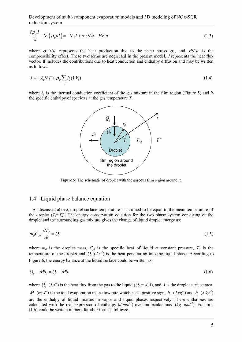
Development of multi-component evaporation models and 3D modeling of NOx-SCR reduction system
5
. . : .gg
IuI J u P u
t
(1.3)
where : u represents the heat production due to the shear stress , and .P u is the compressibility effect. These two terms are neglected in the present model. J represents the heat flux vector. It includes the contributions due to heat conduction and enthalpy diffusion and may be written as follows:
( )g g i i ii
J T h YV (1.4)
where λg is the thermal conduction coefficient of the gas mixture in the film region (Figure 5) and hi the specific enthalpy of species i at the gas temperature T.
Figure 5: The schematic of droplet with the gaseous film region around it.
1.4 Liquid phase balance equation As discussed above, droplet surface temperature is assumed to be equal to the mean temperature of the droplet (Ts=Td). The energy conservation equation for the two phase system consisting of the droplet and the surrounding gas mixture gives the change of liquid droplet energy as:
dd pf l
dTm C Qdt
(1.5)
where md is the droplet mass, Cpf is the specific heat of liquid at constant pressure, Td is the temperature of the droplet and lQ (J.s-1) is the heat penetrating into the liquid phase. According to Figure 6, the energy balance at the liquid surface could be written as:
g v l lQ Mh Q Mh (1.6) where gQ (J.s-1) is the heat flux from the gas to the liquid (Qg = J.A), and A is the droplet surface area.
M (kg.s-1) is the total evaporation mass flow rate which has a positive sign. vh (J.kg-1) and lh (J.kg-1) are the enthalpy of liquid mixture in vapor and liquid phases respectively. These enthalpies are calculated with the real expression of enthalpy (J.mol-1) over molecular mass (kg. mol-1). Equation (1.6) could be written in more familiar form as follows:
lQ
gQ
m
dr
dT refT T
r
Droplet
film region around the droplet
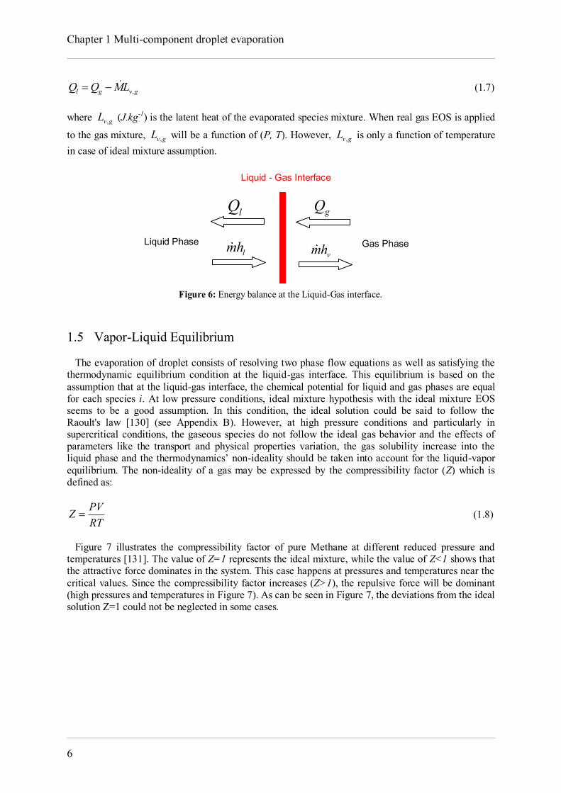
Chapter 1 Multi-component droplet evaporation
6
,l g v gQ Q ML (1.7) where ,v gL (J.kg-1) is the latent heat of the evaporated species mixture. When real gas EOS is applied
to the gas mixture, ,v gL will be a function of (P, T). However, ,v gL is only a function of temperature in case of ideal mixture assumption.
Figure 6: Energy balance at the Liquid-Gas interface.
1.5 Vapor-Liquid Equilibrium The evaporation of droplet consists of resolving two phase flow equations as well as satisfying the thermodynamic equilibrium condition at the liquid-gas interface. This equilibrium is based on the assumption that at the liquid-gas interface, the chemical potential for liquid and gas phases are equal for each species i. At low pressure conditions, ideal mixture hypothesis with the ideal mixture EOS seems to be a good assumption. In this condition, the ideal solution could be said to follow the Raoult's law [130] (see Appendix B). However, at high pressure conditions and particularly in supercritical conditions, the gaseous species do not follow the ideal gas behavior and the effects of parameters like the transport and physical properties variation, the gas solubility increase into the liquid phase and the thermodynamics’ non-ideality should be taken into account for the liquid-vapor equilibrium. The non-ideality of a gas may be expressed by the compressibility factor (Z) which is defined as:
PVZRT
(1.8)
Figure 7 illustrates the compressibility factor of pure Methane at different reduced pressure and temperatures [131]. The value of Z=1 represents the ideal mixture, while the value of Z<1 shows that the attractive force dominates in the system. This case happens at pressures and temperatures near the critical values. Since the compressibility factor increases (Z>1), the repulsive force will be dominant (high pressures and temperatures in Figure 7). As can be seen in Figure 7, the deviations from the ideal solution Z=1 could not be neglected in some cases.
gQlQ
vmhlmh
Liquid - Gas Interface
Gas Phase Liquid Phase
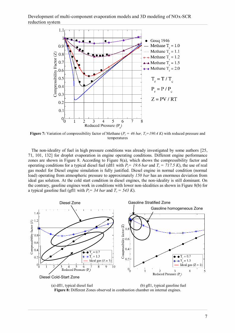
Development of multi-component evaporation models and 3D modeling of NOx-SCR reduction system
7
Figure 7: Variation of compressibility factor of Methane (Pc = 46 bar, Tc=190.4 K) with reduced pressure and
temperatures
The non-ideality of fuel in high pressure conditions was already investigated by some authors [25, 71, 101, 132] for droplet evaporation in engine operating conditions. Different engine performance zones are shown in Figure 8. According to Figure 8(a), which shows the compressibility factor and operating conditions for a typical diesel fuel (dfl1 with Pc= 19.6 bar and Tc = 717.5 K), the use of real gas model for Diesel engine simulation is fully justified. Diesel engine in normal condition (normal load) operating from atmospheric pressure to approximately 150 bar has an enormous deviation from ideal gas solution. At the cold start condition in diesel engines, the non-ideality is still dominant. On the contrary, gasoline engines work in conditions with lower non-idealities as shown in Figure 8(b) for a typical gasoline fuel (gfl1 with Pc= 34 bar and Tc = 543 K).
(a) dfl1, typical diesel fuel (b) gfl1, typical gasoline fuel Figure 8: Different Zones observed in combustion chamber on internal engines.
Diesel Zone
Diesel Cold-Start Zone
Gasoline Stratified Zone Gasoline homogeneous Zone
Chapter 1 Multi-component droplet evaporation
8
In this work, both ideal and real gases EOS are evaluated. They are used especially to determine the mass fraction of gas species at droplets surface as well as latent heat of vaporization. The complete procedure is presented in Appendix B using the well-known Peng-Robinson (PR) cubic EOS [133]. 1.6 Mass flow rate Based on the previous works, some authors [16, 25] have considered the gaseous boundary layer around the droplet to evaluate heat and mass fluxes. These models give the instantaneous droplet vaporization rate from the integration of the quasi-steady species balance around the droplet. By definition [127], the diffusion velocity in Equation (1.1) has to obey the following constraint:
10
N
i ii
YV
(1.9)
Furthermore, the sum of mass fractions must be unity:
11
N
ii
Y
(1.10)
Considering Equations (1.1) and (1.10), there are N unknowns (Yi) with N+1 equations. Thus, the system is over determined. However, if all species of Equation (1.1) are added and the identity of Equation (1.9) is used, the mass conservation equation (Equation (1.2)) is recovered:
1
. . 0N
gg g i i
iu YV
t
(1.11)
Solving the above equation with the general diffusion velocity is too complex and most codes use Hirschfelder's law [125, 134] in the following form:
i i ig iV X D X (1.12) where X is the mole fraction of species i and Dig the diffusion coefficient of species i into the gas mixture. In the present study, the above Hirschfelder's law will be used in the form of mass fraction to be compatible with the model. Using the following relation between the mole fraction and mass fraction of species i :
i ii
WX YW
(1.13)
the Hirschfelder's law may be written using the mass fraction gradient of species i as:
1
1N
ki i ig i i i
k kk i
XVY D X Y YY
(1.14)
The procedure of obtaining Equation (1.14) is given in Appendix C. Using the Hirschfelder's law, the summation of Equation (1.1) over the N gaseous species gives the global mass conservation equation as:
Development of multi-component evaporation models and 3D modeling of NOx-SCR reduction system
9
1 1
. 1N N
g kg g ig i i i
i k kk i
Xu D X Y Yt Y
(1.15)
where the right hand side of the above equation is not zero, unless the diffusion coefficients Dig are assumed to have the same value for all species (this is the case of the KIVA code [135] for instance). Thus, the global mass conservation may not be ensured. One method to implement Hirschfelder's law with different diffusion coefficients while maintaining global mass conservation is to add a correction velocity uc [127] to the absolute velocity in the species Equation (1.1):
1
. 1N
g i c kg i g ig i i i
k kk i
Y XY u u D X Y Yt Y
(1.16)
If all species equations are summed, the mass conservation equation must be recovered:
1 1
. 1 0N N
g ckg g ig i i i g
i k kk i
Xu D X Y Y ut Y
. (1.17)
Thus,
1 1
1N N
c kig i i i
i k kk i
Xu D X Y YY
. (1.18)
Assuming quasi-steady evaporation and integrating Equation (1.17) for liquid species leads to the mean droplet vaporization rate:
2
14
lN
i d gi
M M r u
(1.19)
where rd is the droplet radius. Integrating Equation (1.16) for liquid species between the droplet surface at rd and infinity (∞) where:
i iY Y (1.20)
0cu u (1.21)
0i
r
Yr
(1.22)
gives the following relation for the mass evaporation rate:
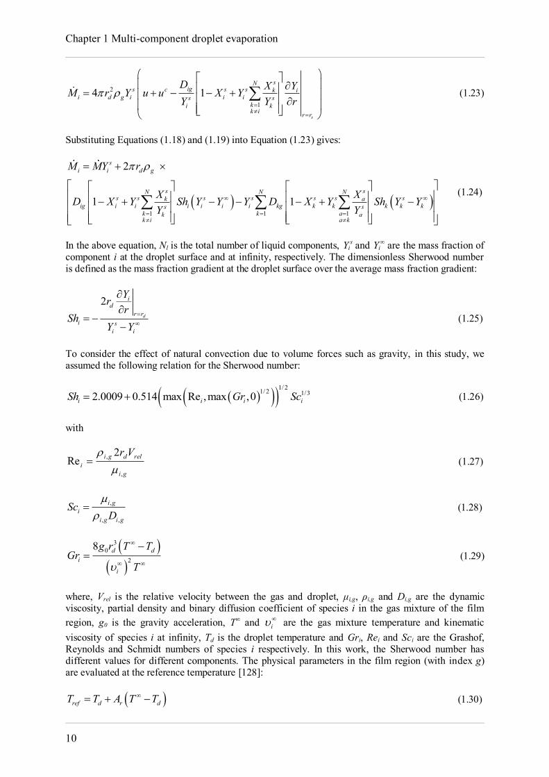
Chapter 1 Multi-component droplet evaporation
10
2
14 1
s
sNigs c s s k i
i d g i i is ski kk i r r
D X YM r Y u u X YY Y r
(1.23)
Substituting Equations (1.18) and (1.19) into Equation (1.23) gives:
1 1 1
2
1 1
si i d g
s sN N Ns s s s s s sk a
ig i i i i i i kg k k k k ks sk k ak ak i a k
M MY r
X XD X Y Sh Y Y Y D X Y Sh Y YY Y
(1.24)
In the above equation, Nl is the total number of liquid components, Yi
s and Yi∞ are the mass fraction of
component i at the droplet surface and at infinity, respectively. The dimensionless Sherwood number is defined as the mass fraction gradient at the droplet surface over the average mass fraction gradient:
2d
id
r ri s
i i
Yrr
ShY Y
(1.25)
To consider the effect of natural convection due to volume forces such as gravity, in this study, we assumed the following relation for the Sherwood number:
1/ 21/ 2 1/32.0009 0.514 max Re ,max ,0i i i iSh Gr Sc (1.26)
with
gi
reldgii
Vr
,
, 2Re
(1.27)
,
, ,
i gi
i g i g
ScD
(1.28)
30
2
8 d di
i
g r T TGr
T
(1.29)
where, Vrel is the relative velocity between the gas and droplet, μi,g, ρi,g and Di,g are the dynamic viscosity, partial density and binary diffusion coefficient of species i in the gas mixture of the film region, g0 is the gravity acceleration, T∞ and i
are the gas mixture temperature and kinematic viscosity of species i at infinity, Td is the droplet temperature and Gri, Rei and Sci are the Grashof, Reynolds and Schmidt numbers of species i respectively. In this work, the Sherwood number has different values for different components. The physical parameters in the film region (with index g) are evaluated at the reference temperature [128]:
ref d r dT T A T T (1.30)
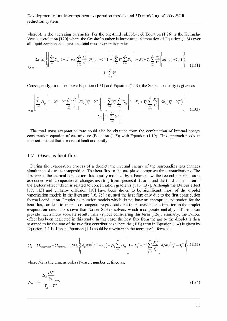
Development of multi-component evaporation models and 3D modeling of NOx-SCR reduction system
11
where Ar is the averaging parameter. For the one-third rule: Ar=1/3. Equation (1.26) is the Kulmala-Vesala correlation [120] where the Grashof number is introduced. Summation of Equation (1.24) over all liquid components, gives the total mass evaporation rate:
1 1 1 1 1
1
2 1 . 1
1
l l
l
N Ns sN N Ns s s s s s sk a
d g ig i i i i i i kg k k k k ks si k i k ak a
k i a k
Ns
ii
X Xr D X Y Sh Y Y Y D X Y Sh Y YY Y
MY
(1.31)
Consequently, from the above Equation (1.31) and Equation (1.19), the Stephan velocity is given as:
1 1 1 1 1
1
1 . 1
2 1
l l
l
N Ns sN N Ns s s s s s sk a
ig i i i i i i kg k k k k ks si k i k ak a
k i a k
Ns
d ii
X XD X Y Sh Y Y Y D X Y Sh Y YY Y
ur Y
(1.32)
The total mass evaporation rate could also be obtained from the combination of internal energy conservation equation of gas mixture (Equation (1.3)) with Equation (1.19). This approach needs an implicit method that is more difficult and costly. 1.7 Gaseous heat flux During the evaporation process of a droplet, the internal energy of the surrounding gas changes simultaneously to its composition. The heat flux in the gas phase comprises three contributions. The first one is the thermal conduction flux usually modeled by a Fourier law; the second contribution is associated with compositional changes resulting from species diffusion; and the third contribution is the Dufour effect which is related to concentration gradients [136, 137]. Although the Dufour effect [89, 113] and enthalpy diffusion [18] have been shown to be significant, most of the droplet vaporization models in the literature [16, 25] assumed the heat flux only due to the first contribution thermal conduction. Droplet evaporation models which do not have an appropriate estimation for the heat flux, can lead to anomalous temperature gradients and to an over/under-estimation in the droplet evaporation rate. It is shown that Navier-Stokes solvers which incorporate enthalpy diffusion can provide much more accurate results than without considering this term [126]. Similarly, the Dufour effect has been neglected in this study. In this case, the heat flux from the gas to the droplet is then assumed to be the sum of the two first contributions where the (YiVi) term in Equation (1.4) is given by Equation (1.14). Hence, Equation (1.4) could be rewritten in the more useful form as:
1 1
2 1lN sN
s s skg conduction enthalpy d g d g ig i i i i i is
i k kk i
XQ Q Q r Nu T T D X Y h Sh Y YY
(1.33)
where Nu is the dimensionless Nusselt number defined as:
2d
dr r
d
Trr
NuT T
(1.34)
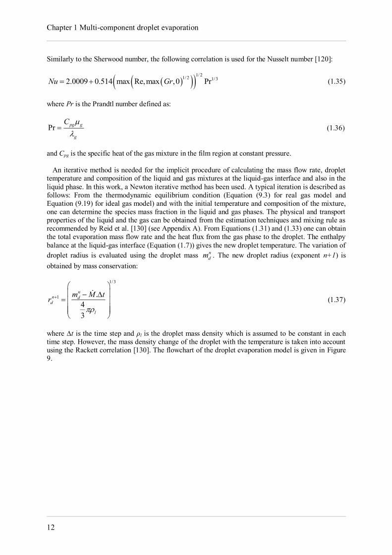
Chapter 1 Multi-component droplet evaporation
12
Similarly to the Sherwood number, the following correlation is used for the Nusselt number [120]:
1/ 21/ 2 1/32.0009 0.514 max Re,max ,0 PrNu Gr (1.35)
where Pr is the Prandtl number defined as:
Pr pg g
g
C
(1.36)
and Cpg is the specific heat of the gas mixture in the film region at constant pressure. An iterative method is needed for the implicit procedure of calculating the mass flow rate, droplet temperature and composition of the liquid and gas mixtures at the liquid-gas interface and also in the liquid phase. In this work, a Newton iterative method has been used. A typical iteration is described as follows: From the thermodynamic equilibrium condition (Equation (9.3) for real gas model and Equation (9.19) for ideal gas model) and with the initial temperature and composition of the mixture, one can determine the species mass fraction in the liquid and gas phases. The physical and transport properties of the liquid and the gas can be obtained from the estimation techniques and mixing rule as recommended by Reid et al. [130] (see Appendix A). From Equations (1.31) and (1.33) one can obtain the total evaporation mass flow rate and the heat flux from the gas phase to the droplet. The enthalpy balance at the liquid-gas interface (Equation (1.7)) gives the new droplet temperature. The variation of droplet radius is evaluated using the droplet mass n
dm . The new droplet radius (exponent n+1) is obtained by mass conservation:
1/3
1 .43
nn d
d
l
m M tr
(1.37)
where ∆t is the time step and ρl is the droplet mass density which is assumed to be constant in each time step. However, the mass density change of the droplet with the temperature is taken into account using the Rackett correlation [130]. The flowchart of the droplet evaporation model is given in Figure 9.
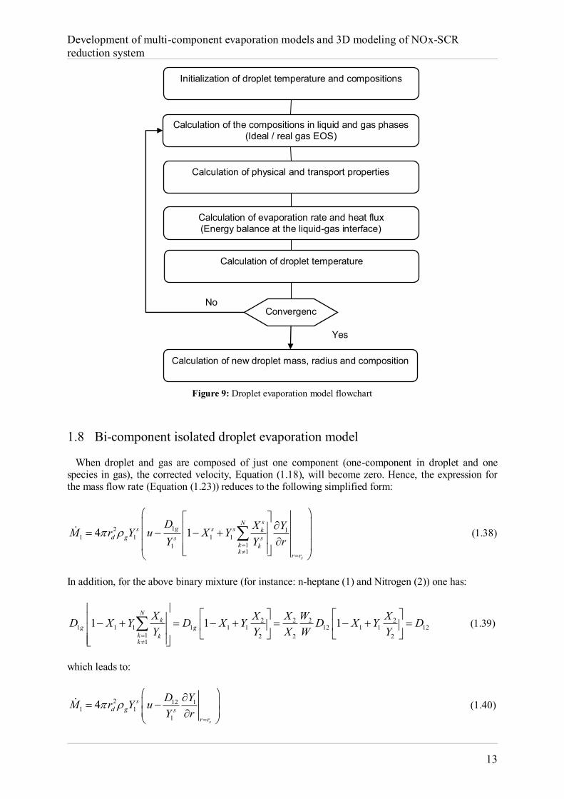
Development of multi-component evaporation models and 3D modeling of NOx-SCR reduction system
13
Figure 9: Droplet evaporation model flowchart
1.8 Bi-component isolated droplet evaporation model When droplet and gas are composed of just one component (one-component in droplet and one species in gas), the corrected velocity, Equation (1.18), will become zero. Hence, the expression for the mass flow rate (Equation (1.23)) reduces to the following simplified form:
12 11 1 1 1
111
4 1
s
sNgs s s k
d g s sk kk r r
D X YM r Y u X YY Y r
(1.38)
In addition, for the above binary mixture (for instance: n-heptane (1) and Nitrogen (2)) one has:
2 2 2 21 1 1 1 1 1 12 1 1 12
1 2 2 21
1 1 1N
kg g
k kk
X X X W XD X Y D X Y D X Y DY Y X W Y
(1.39)
which leads to:
2 12 11 1
1
4s
sd g s
r r
D YM r Y uY r
(1.40)
Initialization of droplet temperature and compositions
Calculation of the compositions in liquid and gas phases (Ideal / real gas EOS)
Calculation of physical and transport properties
Calculation of evaporation rate and heat flux (Energy balance at the liquid-gas interface)
Calculation of droplet temperature
Calculation of new droplet mass, radius and composition
Convergence
Yes
No
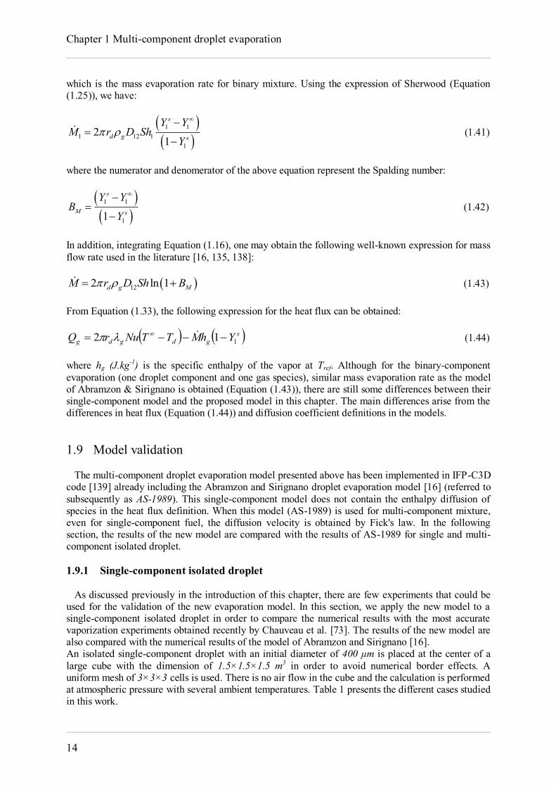
Chapter 1 Multi-component droplet evaporation
14
which is the mass evaporation rate for binary mixture. Using the expression of Sherwood (Equation (1.25)), we have:
1 11 12 1
1
21
s
d g s
Y YM r D Sh
Y
(1.41)
where the numerator and denomerator of the above equation represent the Spalding number:
1 1
11
s
M s
Y YB
Y
(1.42)
In addition, integrating Equation (1.16), one may obtain the following well-known expression for mass flow rate used in the literature [16, 135, 138]:
122 ln 1d g MM r D Sh B (1.43) From Equation (1.33), the following expression for the heat flux can be obtained:
sgdgdg YhMTTNurQ 112 (1.44)
where hg (J.kg-1) is the specific enthalpy of the vapor at Tref. Although for the binary-component evaporation (one droplet component and one gas species), similar mass evaporation rate as the model of Abramzon & Sirignano is obtained (Equation (1.43)), there are still some differences between their single-component model and the proposed model in this chapter. The main differences arise from the differences in heat flux (Equation (1.44)) and diffusion coefficient definitions in the models. 1.9 Model validation The multi-component droplet evaporation model presented above has been implemented in IFP-C3D code [139] already including the Abramzon and Sirignano droplet evaporation model [16] (referred to subsequently as AS-1989). This single-component model does not contain the enthalpy diffusion of species in the heat flux definition. When this model (AS-1989) is used for multi-component mixture, even for single-component fuel, the diffusion velocity is obtained by Fick's law. In the following section, the results of the new model are compared with the results of AS-1989 for single and multi-component isolated droplet. 1.9.1 Single-component isolated droplet As discussed previously in the introduction of this chapter, there are few experiments that could be used for the validation of the new evaporation model. In this section, we apply the new model to a single-component isolated droplet in order to compare the numerical results with the most accurate vaporization experiments obtained recently by Chauveau et al. [73]. The results of the new model are also compared with the numerical results of the model of Abramzon and Sirignano [16]. An isolated single-component droplet with an initial diameter of 400 μm is placed at the center of a large cube with the dimension of 1.5×1.5×1.5 m3 in order to avoid numerical border effects. A uniform mesh of 3×3×3 cells is used. There is no air flow in the cube and the calculation is performed at atmospheric pressure with several ambient temperatures. Table 1 presents the different cases studied in this work.
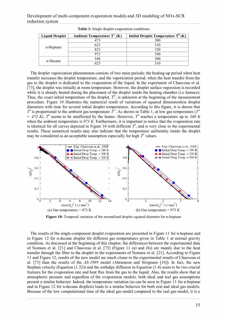
Development of multi-component evaporation models and 3D modeling of NOx-SCR reduction system
15
Table 1: Single droplet evaporation conditions
Liquid Droplet Ambient Temperature T∞ (K) Initial Droplet Temperature T0 (K)
n-Heptane
473 300 623 310 823 320 973 340
n-Decane 548 300 623 310
The droplet vaporization phenomenon consists of two main periods; the heating-up period when heat transfer increases the droplet temperature, and the vaporization period, when the heat transfer from the gas to the droplet is dedicated to the evaporation of the liquid. In the experiment of Chauveau et al. [73], the droplet was initially at room temperature. However, the droplet surface regression is recorded while it is already heated during the placement of the droplet inside the heating chamber (i.e furnace). Thus, the exact initial temperature of the droplet, T0, is unknown at the beginning of the measurement procedure. Figure 10 illustrates the numerical result of variations of squared dimensionless droplet diameters with time for several initial droplet temperatures. According to this figure, it is shown that T0 is proportional to the ambient gas temperature T∞. As shown in Table 1, at low gas temperature (T∞
= 473 K), T0 seems to be unaffected by the heater. However, T0 reaches a temperature up to 340 K when the ambient temperature is 973 K. Furthermore, it is important to notice that the evaporation rate is identical for all curves depicted in Figure 10 with different T0, and is very close to the experimental results. These numerical results may also indicate that the temperature uniformity inside the droplet may be considered as an acceptable assumption especially for high T0 values.
(a) Gas temperature = 473 K (b) Gas temperature = 973 K
Figure 10: Temporal variation of the normalized droplet squared diameter for n-heptane
The results of the single-component droplet evaporation are presented in Figure 11 for n-heptane and in Figure 12 for n-decane droplet for different gas temperatures given in Table 1 at normal gravity condition. As discussed at the beginning of this chapter, the differences between the experimental data of Nomura et al. [21] and Chauveau et al. [73] (Figure 11 (a) and (b)) are mainly due to the heat transfer through the fiber to the droplet in the experiments of Nomura et al. [21]. According to Figure 11 and Figure 12, results of the new model are much closer to the experimental results of Chauveau et al. [73] than the results of the AS-1989 model (Abramzon and Sirignano [16]). In fact, the new Stephan velocity (Equation (1.32)) and the enthalpy diffusion in Equation (1.4) seem to be two crucial features for the evaporation rate and heat flux from the gas to the liquid. Also, the results show that at atmospheric pressure and regardless of the evaporation models, both ideal and real gas assumptions present a similar behavior. Indeed, the temperature variation (as can be seen in Figure 11 for n-heptane and in Figure 12 for n-decane droplets) leads to a similar behavior for both real and ideal gas models. Because of the low computational time of the ideal gas model compared to the real gas model, it is a
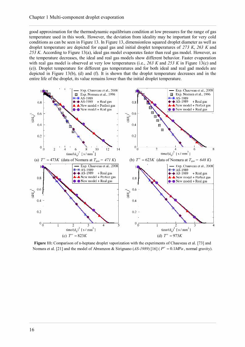
Chapter 1 Multi-component droplet evaporation
16
good approximation for the thermodynamic equilibrium condition at low pressures for the range of gas temperature used in this work. However, the deviation from ideality may be important for very cold conditions as can be seen in Figure 13. In Figure 13, dimensionless squared droplet diameter as well as droplet temperature are depicted for equal gas and initial droplet temperatures of 273 K, 263 K and 253 K. According to Figure 13(a), ideal gas model evaporates faster than real gas model. However, as the temperature decreases, the ideal and real gas models show different behavior. Faster evaporation with real gas model is observed at very low temperatures (i.e., 263 K and 253 K in Figure 13(c) and (e)). Droplet temperature for different gas temperatures and for both ideal and real gad models are depicted in Figure 13(b), (d) and (f). It is shown that the droplet temperature decreases and in the entire life of the droplet, its value remains lower than the initial droplet temperature.
(a) 473T K (data of Nomura at Tgas = 471 K) (b) 623T K (data of Nomura at Tgas = 648 K)
(c) 823T K (d) 973T K
Figure 11: Comparison of n-heptane droplet vaporization with the experiments of Chauveau et al. [73] and Nomura et al. [21] and the model of Abramzon & Sirignano (AS-1989) [16] ( 0.1P MPa , normal gravity).
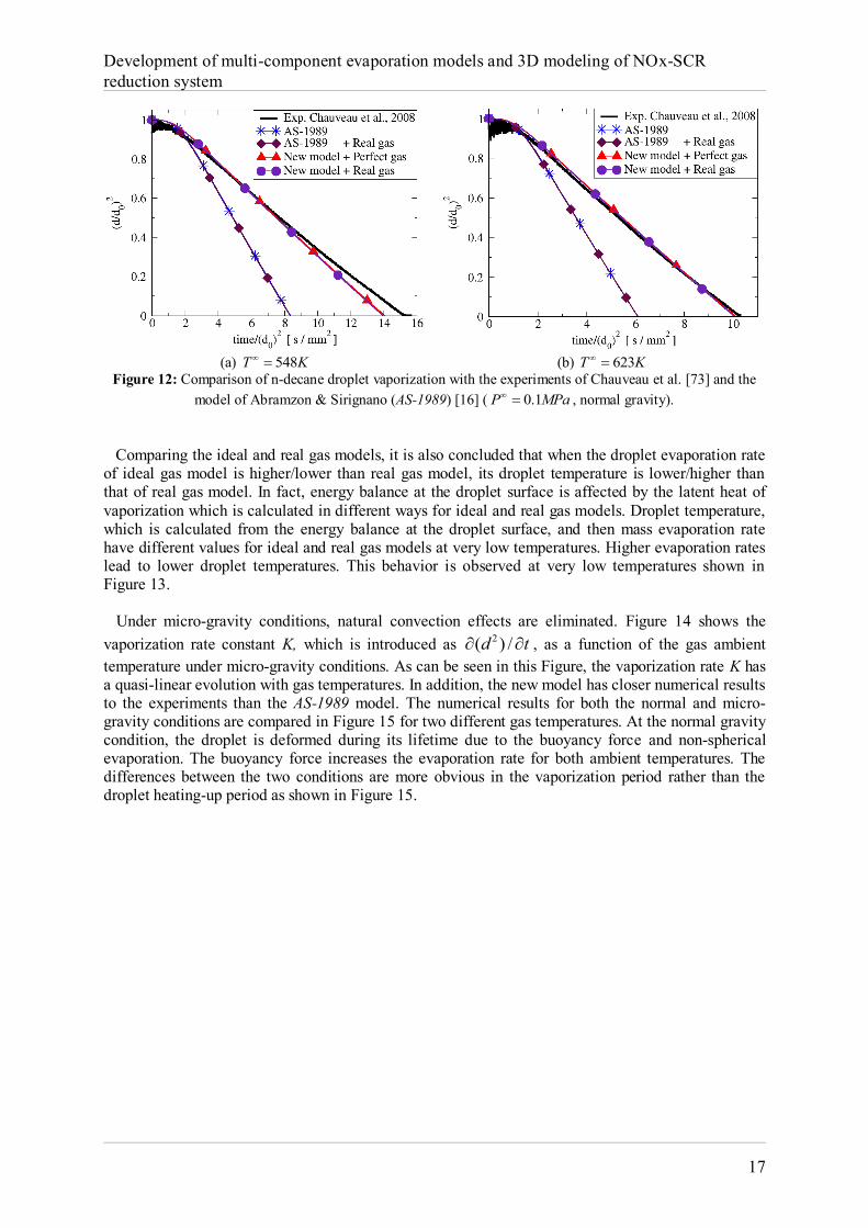
Development of multi-component evaporation models and 3D modeling of NOx-SCR reduction system
17
(a) 548T K (b) 623T K
Figure 12: Comparison of n-decane droplet vaporization with the experiments of Chauveau et al. [73] and the model of Abramzon & Sirignano (AS-1989) [16] ( 0.1P MPa , normal gravity).
Comparing the ideal and real gas models, it is also concluded that when the droplet evaporation rate of ideal gas model is higher/lower than real gas model, its droplet temperature is lower/higher than that of real gas model. In fact, energy balance at the droplet surface is affected by the latent heat of vaporization which is calculated in different ways for ideal and real gas models. Droplet temperature, which is calculated from the energy balance at the droplet surface, and then mass evaporation rate have different values for ideal and real gas models at very low temperatures. Higher evaporation rates lead to lower droplet temperatures. This behavior is observed at very low temperatures shown in Figure 13. Under micro-gravity conditions, natural convection effects are eliminated. Figure 14 shows the vaporization rate constant K, which is introduced as 2( ) /d t , as a function of the gas ambient temperature under micro-gravity conditions. As can be seen in this Figure, the vaporization rate K has a quasi-linear evolution with gas temperatures. In addition, the new model has closer numerical results to the experiments than the AS-1989 model. The numerical results for both the normal and micro-gravity conditions are compared in Figure 15 for two different gas temperatures. At the normal gravity condition, the droplet is deformed during its lifetime due to the buoyancy force and non-spherical evaporation. The buoyancy force increases the evaporation rate for both ambient temperatures. The differences between the two conditions are more obvious in the vaporization period rather than the droplet heating-up period as shown in Figure 15.
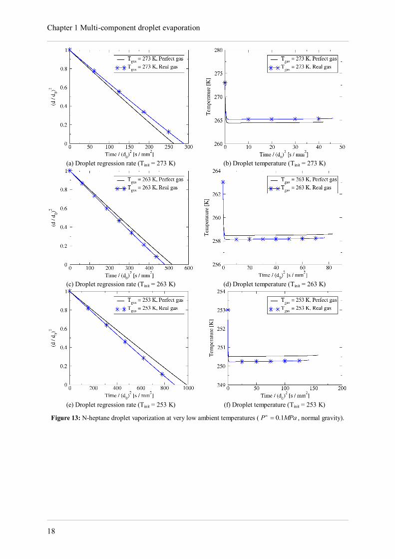
Chapter 1 Multi-component droplet evaporation
18
(a) Droplet regression rate (Tinit = 273 K) (b) Droplet temperature (Tinit = 273 K)
(c) Droplet regression rate (Tinit = 263 K) (d) Droplet temperature (Tinit = 263 K)
(e) Droplet regression rate (Tinit = 253 K) (f) Droplet temperature (Tinit = 253 K)
Figure 13: N-heptane droplet vaporization at very low ambient temperatures ( 0.1P MPa , normal gravity).
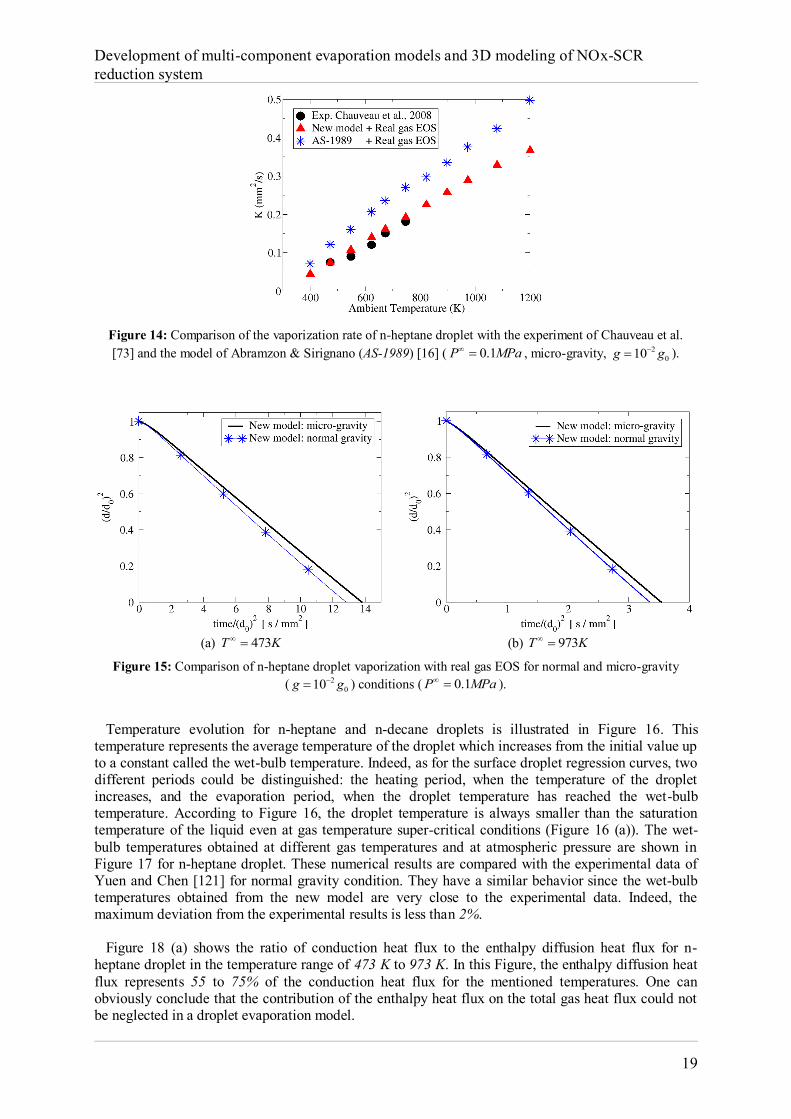
Development of multi-component evaporation models and 3D modeling of NOx-SCR reduction system
19
Figure 14: Comparison of the vaporization rate of n-heptane droplet with the experiment of Chauveau et al. [73] and the model of Abramzon & Sirignano (AS-1989) [16] ( 0.1P MPa , micro-gravity, 2
010g g ).
(a) 473T K (b) 973T K
Figure 15: Comparison of n-heptane droplet vaporization with real gas EOS for normal and micro-gravity ( 2
010g g ) conditions ( 0.1P MPa ).
Temperature evolution for n-heptane and n-decane droplets is illustrated in Figure 16. This temperature represents the average temperature of the droplet which increases from the initial value up to a constant called the wet-bulb temperature. Indeed, as for the surface droplet regression curves, two different periods could be distinguished: the heating period, when the temperature of the droplet increases, and the evaporation period, when the droplet temperature has reached the wet-bulb temperature. According to Figure 16, the droplet temperature is always smaller than the saturation temperature of the liquid even at gas temperature super-critical conditions (Figure 16 (a)). The wet-bulb temperatures obtained at different gas temperatures and at atmospheric pressure are shown in Figure 17 for n-heptane droplet. These numerical results are compared with the experimental data of Yuen and Chen [121] for normal gravity condition. They have a similar behavior since the wet-bulb temperatures obtained from the new model are very close to the experimental data. Indeed, the maximum deviation from the experimental results is less than 2%. Figure 18 (a) shows the ratio of conduction heat flux to the enthalpy diffusion heat flux for n-heptane droplet in the temperature range of 473 K to 973 K. In this Figure, the enthalpy diffusion heat flux represents 55 to 75% of the conduction heat flux for the mentioned temperatures. One can obviously conclude that the contribution of the enthalpy heat flux on the total gas heat flux could not be neglected in a droplet evaporation model.
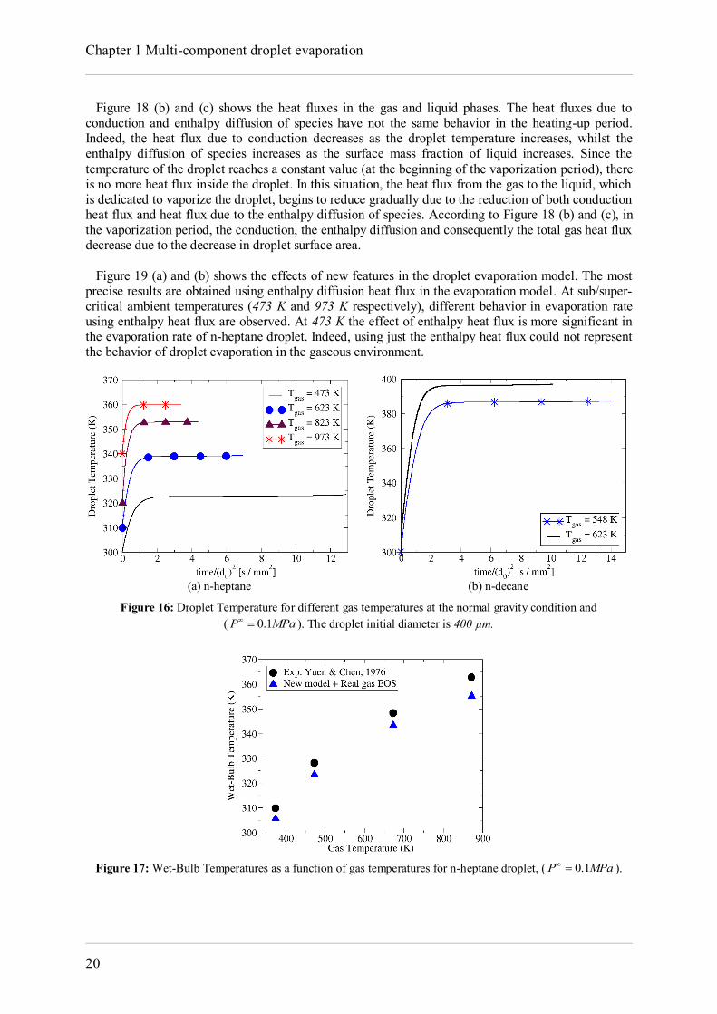
Chapter 1 Multi-component droplet evaporation
20
Figure 18 (b) and (c) shows the heat fluxes in the gas and liquid phases. The heat fluxes due to conduction and enthalpy diffusion of species have not the same behavior in the heating-up period. Indeed, the heat flux due to conduction decreases as the droplet temperature increases, whilst the enthalpy diffusion of species increases as the surface mass fraction of liquid increases. Since the temperature of the droplet reaches a constant value (at the beginning of the vaporization period), there is no more heat flux inside the droplet. In this situation, the heat flux from the gas to the liquid, which is dedicated to vaporize the droplet, begins to reduce gradually due to the reduction of both conduction heat flux and heat flux due to the enthalpy diffusion of species. According to Figure 18 (b) and (c), in the vaporization period, the conduction, the enthalpy diffusion and consequently the total gas heat flux decrease due to the decrease in droplet surface area. Figure 19 (a) and (b) shows the effects of new features in the droplet evaporation model. The most precise results are obtained using enthalpy diffusion heat flux in the evaporation model. At sub/super-critical ambient temperatures (473 K and 973 K respectively), different behavior in evaporation rate using enthalpy heat flux are observed. At 473 K the effect of enthalpy heat flux is more significant in the evaporation rate of n-heptane droplet. Indeed, using just the enthalpy heat flux could not represent the behavior of droplet evaporation in the gaseous environment.
(a) n-heptane (b) n-decane
Figure 16: Droplet Temperature for different gas temperatures at the normal gravity condition and ( 0.1P MPa ). The droplet initial diameter is 400 µm.
Figure 17: Wet-Bulb Temperatures as a function of gas temperatures for n-heptane droplet, ( 0.1P MPa ).
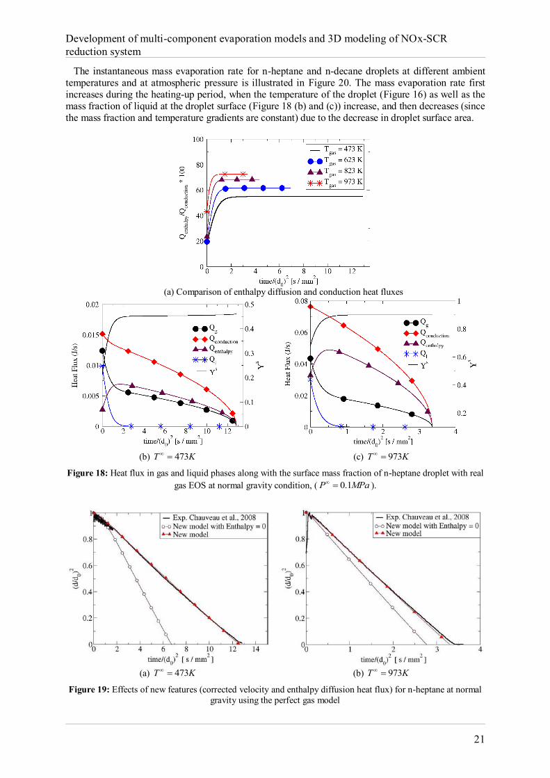
Development of multi-component evaporation models and 3D modeling of NOx-SCR reduction system
21
The instantaneous mass evaporation rate for n-heptane and n-decane droplets at different ambient temperatures and at atmospheric pressure is illustrated in Figure 20. The mass evaporation rate first increases during the heating-up period, when the temperature of the droplet (Figure 16) as well as the mass fraction of liquid at the droplet surface (Figure 18 (b) and (c)) increase, and then decreases (since the mass fraction and temperature gradients are constant) due to the decrease in droplet surface area.
(a) Comparison of enthalpy diffusion and conduction heat fluxes
(b) 473T K (c) 973T K
Figure 18: Heat flux in gas and liquid phases along with the surface mass fraction of n-heptane droplet with real gas EOS at normal gravity condition, ( 0.1P MPa ).
(a) 473T K (b) 973T K
Figure 19: Effects of new features (corrected velocity and enthalpy diffusion heat flux) for n-heptane at normal gravity using the perfect gas model
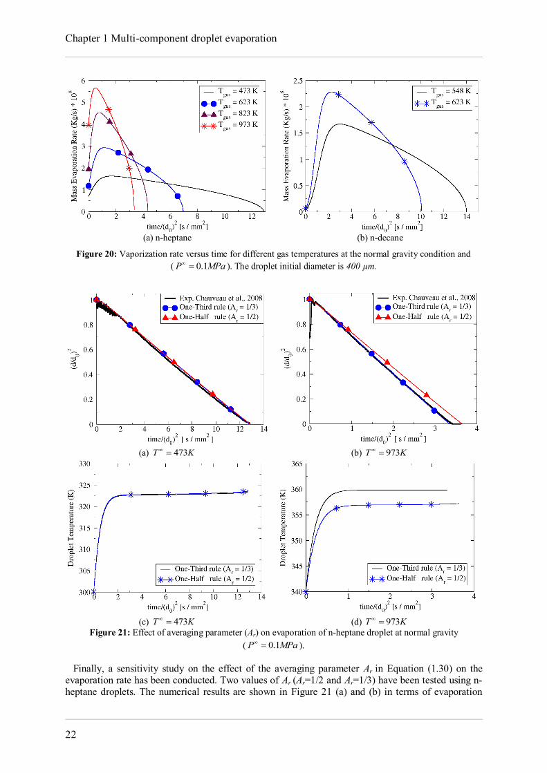
Chapter 1 Multi-component droplet evaporation
22
(a) n-heptane (b) n-decane
Figure 20: Vaporization rate versus time for different gas temperatures at the normal gravity condition and ( 0.1P MPa ). The droplet initial diameter is 400 µm.
(a) 473T K (b) 973T K
(c) 473T K (d) 973T K
Figure 21: Effect of averaging parameter (Ar) on evaporation of n-heptane droplet at normal gravity ( 0.1P MPa ).
Finally, a sensitivity study on the effect of the averaging parameter Ar in Equation (1.30) on the evaporation rate has been conducted. Two values of Ar (Ar=1/2 and Ar=1/3) have been tested using n-heptane droplets. The numerical results are shown in Figure 21 (a) and (b) in terms of evaporation
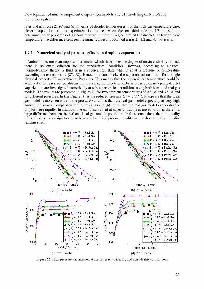
Development of multi-component evaporation models and 3D modeling of NOx-SCR reduction system
23
rates and in Figure 21 (c) and (d) in terms of droplet temperatures. For the high gas temperature case, closer evaporation rate to experiment is obtained when the one-third rule Ar=1/3 is used for determination of properties of gaseous mixture in the film region around the droplet. At low ambient temperature, the difference between the numerical results obtained using Ar=1/2 and Ar=1/3 is small. 1.9.2 Numerical study of pressure effects on droplet evaporation Ambient pressure is an important parameter which determines the degree of mixture ideality. In fact, there is no exact criterion for the supercritical condition. However, according to classical thermodynamic theory, a fluid is in a supercritical state when it is at a pressure or temperature exceeding its critical value [87, 88]. Hence, one can invoke the supercritical condition for a single physical property (Temperature or Pressure). This means that the supercritical temperature could be achieved at low pressure conditions. In this work, the effects of ambient pressure on n-heptane droplet vaporization are investigated numerically at sub/super-critical conditions using both ideal and real gas models. The results are presented in Figure 22 for two ambient temperatures of 473 K and 973 K and for different pressures. In this Figure, Pr is the reduced pressure (Pr = P / Pc). It appears that the ideal gas model is more sensitive to the pressure variations than the real gas model especially at very high ambient pressures. Comparison of Figure 22 (a) and (b) shows that the real gas model evaporates the droplet more rapidly. In addition, one can observe that at super-critical pressure conditions, there is a large difference between the real and ideal gas models prediction. In these conditions, the non-ideality of the fluid becomes significant. At low or sub-critical pressure conditions, the deviation from ideality remains small.
(a) 473T K (b) 973T K
(c) 473T K (d) 973T K
Figure 22: High-pressure vaporization at normal gravity; ideality and non-ideality comparisons
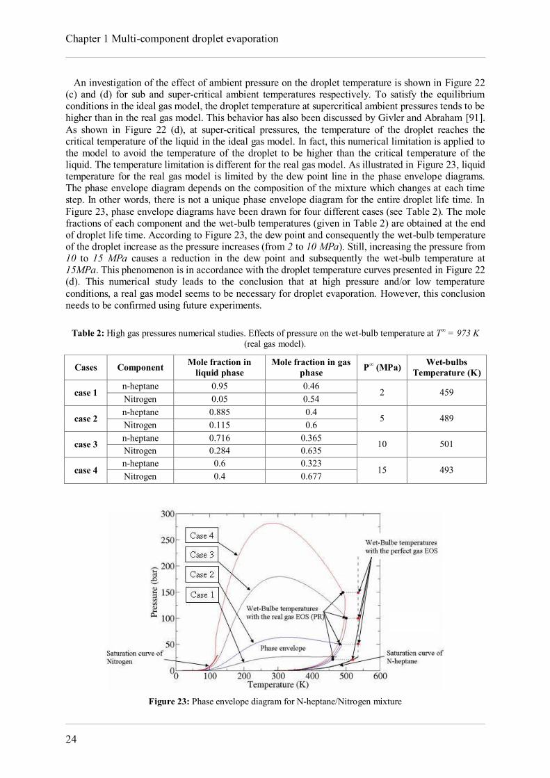
Chapter 1 Multi-component droplet evaporation
24
An investigation of the effect of ambient pressure on the droplet temperature is shown in Figure 22 (c) and (d) for sub and super-critical ambient temperatures respectively. To satisfy the equilibrium conditions in the ideal gas model, the droplet temperature at supercritical ambient pressures tends to be higher than in the real gas model. This behavior has also been discussed by Givler and Abraham [91]. As shown in Figure 22 (d), at super-critical pressures, the temperature of the droplet reaches the critical temperature of the liquid in the ideal gas model. In fact, this numerical limitation is applied to the model to avoid the temperature of the droplet to be higher than the critical temperature of the liquid. The temperature limitation is different for the real gas model. As illustrated in Figure 23, liquid temperature for the real gas model is limited by the dew point line in the phase envelope diagrams. The phase envelope diagram depends on the composition of the mixture which changes at each time step. In other words, there is not a unique phase envelope diagram for the entire droplet life time. In Figure 23, phase envelope diagrams have been drawn for four different cases (see Table 2). The mole fractions of each component and the wet-bulb temperatures (given in Table 2) are obtained at the end of droplet life time. According to Figure 23, the dew point and consequently the wet-bulb temperature of the droplet increase as the pressure increases (from 2 to 10 MPa). Still, increasing the pressure from 10 to 15 MPa causes a reduction in the dew point and subsequently the wet-bulb temperature at 15MPa. This phenomenon is in accordance with the droplet temperature curves presented in Figure 22 (d). This numerical study leads to the conclusion that at high pressure and/or low temperature conditions, a real gas model seems to be necessary for droplet evaporation. However, this conclusion needs to be confirmed using future experiments.
Table 2: High gas pressures numerical studies. Effects of pressure on the wet-bulb temperature at T∞ = 973 K (real gas model).
Cases Component Mole fraction in liquid phase
Mole fraction in gas phase P∞ (MPa) Wet-bulbs
Temperature (K)
case 1 n-heptane 0.95 0.46
2 459 Nitrogen 0.05 0.54
case 2 n-heptane 0.885 0.4
5 489 Nitrogen 0.115 0.6
case 3 n-heptane 0.716 0.365 10 501 Nitrogen 0.284 0.635
case 4 n-heptane 0.6 0.323
15 493 Nitrogen 0.4 0.677
Figure 23: Phase envelope diagram for N-heptane/Nitrogen mixture
Development of multi-component evaporation models and 3D modeling of NOx-SCR reduction system
25
1.9.3 Multi-component isolated droplet To evaluate its accuracy for multi-component liquids, the model is also applied to the experiment of Birouk [122], evaporating a two-component droplet made up of a mixture of n-heptane and n-decane in nitrogen environment at a temperature of 293 K and a pressure of 0.1 MPa. In the experiment of Birouk [122], the droplet is suspended on a vertical quartz fiber with 0.2 mm diameter and the temperature of the drop is initially of 293 K. Although the experiments of Birouk have been obtained using a thick quartz fiber, they seem to be sufficiently accurate at such low ambient temperature (293 K). The numerical results obtained for the stagnant condition are presented in Figure 24. A classical distillation is obtained. In the numerical results, the most volatile component (n-heptane) is first completely depleted, followed by n-decane evaporation. Indeed, in Figure 24 the numerical results show that the evaporation of n-decane starts later than in the experiment. To explain this behavior, we have introduced a virtual diameter dn-decane which is proportional to the initial volume fraction of n-decane n-decane in the droplet. In Figure 24 (a), the value of n-decane = 0.3 leads to a virtual diameter for n-decane dn-decane=0.669d0 and (dn-decane/d0)2 ≈ 0.45. Hence, n-decane should evaporate alone as a single-component, at least when (d/d0)2 reaches the value of 0.45. Actually, n-decane begins to evaporate in the same time as n-heptane (at the beginning of the evaporation process) with less evaporation rate which causes a reduction of the virtual diameter dn-decane. Thus, the evaporation of n-decane should begin at (d/d0)2<0.45. This behavior is well represented in Figure 24 (a) as well as in Figure 24 (b) for the numerical model. This reasoning leads to the conclusion that the initial volume fraction of n-decane in droplets was probably overestimated by Birouk [122] in their experiments. A probable scenario may be that a certain fraction of n-heptane was already evaporated before the beginning of the measurement procedure of Birouk [122]. Reconsidering Figure 24 (a) with a new initial composition of liquid mixture (65% n-heptane) in the numerical calculation shows closer behavior between the numerical results and experimental data. The second point that has to be discussed here concerns the evaporation rate of n-heptane component. The results of Birouk [122] shows faster evaporation of the first component (n-heptane) which is due to the effects of heat conduction through the fiber. As can be seen in Figure 24 (c), droplet temperature decreases at the beginning of evaporation process and then increases to the ambient temperature. In the first part of the temperature curve (part 1: which mostly corresponds to the evaporation of n-heptane), the differences between the droplet temperature and ambient temperature cause the heat flux through the fiber to be important. Since the second component (n-decane) starts to evaporate alone, there is not a significant temperature difference between the droplet and the ambient gas. Thus, the effect of conduction heat flux through the fiber is negligible in part 2 (Figure 24(c)). This explains why the slopes of the experimental and numerical curves in the second part of Figure 24 (a) are identical. A second multi-component test case was performed, based on the experimental data of Brenn et al. [19] for multi-component biofuel droplets. The numerical results of five-component droplet evaporation with initial diameter of 1.72 mm, obtained for an acoustically levitated droplet, are depicted in Figure 25. In this case, atmospheric pressure condition with ambient air temperature of 304 K and a relative humidity of 2% are applied. Figure 25 reveals a good agreement between the computational results and the experimental data. The numerical results shown in Figure 25 are obtained using the ideal mixture EOS at the liquid-gas interface (Raoult's law [130] and Appendix B). However, to satisfy the thermodynamic equilibrium condition for oxygenated hydrocarbons (like methanol, ethanol and 1-butanol), an appropriate EOS like cubic plus association (CPA) (Refs. [140-144]) should be used in order to improve the present model.
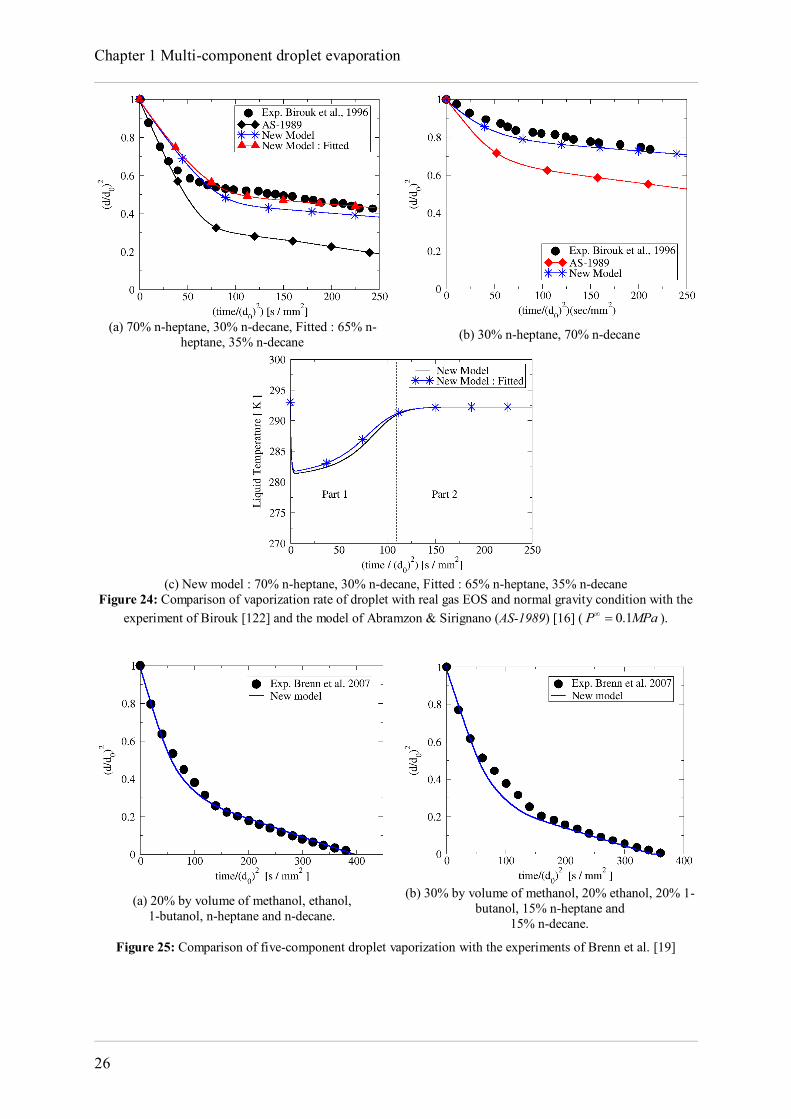
Chapter 1 Multi-component droplet evaporation
26
(a) 70% n-heptane, 30% n-decane, Fitted : 65% n-
heptane, 35% n-decane (b) 30% n-heptane, 70% n-decane
(c) New model : 70% n-heptane, 30% n-decane, Fitted : 65% n-heptane, 35% n-decane
Figure 24: Comparison of vaporization rate of droplet with real gas EOS and normal gravity condition with the experiment of Birouk [122] and the model of Abramzon & Sirignano (AS-1989) [16] ( 0.1P MPa ).
(a) 20% by volume of methanol, ethanol,
1-butanol, n-heptane and n-decane.
(b) 30% by volume of methanol, 20% ethanol, 20% 1-butanol, 15% n-heptane and
15% n-decane.
Figure 25: Comparison of five-component droplet vaporization with the experiments of Brenn et al. [19]

Development of multi-component evaporation models and 3D modeling of NOx-SCR reduction system
27
1.10 Conclusions A new multi-component droplet evaporation model has been proposed in this chapter [145]. It is based on a new Stephan velocity which recovers the mass conservation equation when Hirschfelder's law is used for the diffusion velocity. In addition, the heat flux is assumed to be the summation of heat conduction and enthalpy diffusion of species. Enthalpy diffusion accounts for energy changes associated with compositional changes resulting from species diffusion. The following conclusions are made: The numerical results of the new model are in very good agreement with the experimental data
of Chauveau et al. [73] at atmospheric pressure. The numerical results have shown that the heat flux due to the enthalpy diffusion of species
could not be neglected in comparison to the conduction heat flux. Infinite thermal conductivity assumption inside the droplet which has been invoked in this study
gives acceptable results compared to the experimental data of Chauveau et al. [73]. The results show that the gravity and consequently, natural convection affects the evaporation
rate of droplets situated in quiescent conditions. A sensitivity study on the choice of the averaging parameter has shown that more satisfying
results are obtained with the one-third rule (Ar = 1/3) at sub and super-critical ambient temperatures.
At low pressure conditions, the ideal gas model could be a good assumption for the droplet vaporization in the range of gas temperatures used in this study. However, at high pressure and/or low temperature conditions, there is a large difference between the real and ideal gas models. This leads to the conclusion that at high pressure conditions, a real gas model that could better represent the thermodynamic equilibrium condition is needed.
The multi-component droplet vaporization model has been applied to a two-component droplet (n-heptane/n-decane) test case. The numerical results are compared with the experimental data of Birouk [122]. It is shown that in both numerical model and experiments, the n-decane (the less volatile component) evaporates with the same evaporation rate. However, this could not be obtained in the evaporation of n-heptane (the most volatile) component. It has been shown that the disagreement may be due to the heat flux through the fiber.
In order to use the present model for biofuels containing oxygenated hydrocarbons, development of vapor-liquid equilibrium with an appropriate EOS is needed. In this case, the activity coefficient may have important effect on the evaporation process.
The proposed model is applied to hydrocarbon droplets. For urea-water solution (UWS) used in SCR systems, vapor-liquid equilibrium with appropriate activity coefficients is also needed. This model is developed in Part 2 of this manuscript.
Chapter 2
Multi-component liquid film evaporation 2.1 Introduction Liquid film evaporation is important phenomenon in internal combustion engines (Diesel and gasoline). Since the spray is directly injected into the combustion chamber, some droplets may hit the cylinder wall and form a thin liquid film. Liquid film formation and evolution have significant effects on engine hydrocarbon (HC) and soot emissions, due to incomplete liquid film evaporation especially at cold start conditions [146-148]. Therefore, studying film formation and evaporation in turbulent gas flow conditions is of great practical significance. The evaporation of liquid film of complex mixtures, containing hundreds of components, is frequently encountered in engineering, particularly in combustors and engines burning commercial petroleum fuels. Lumping together all species into a single fuel model is a simplified way to use single-component evaporation models in order to reduce the computational time [30, 149]. However, this approach may lead to important uncertainty in the numerical results, especially in cold start engine conditions for instance [3, 4]. Indeed, in this case the most volatile fraction of the fuel evaporates first and plays an important role in the initial ignition. However, this distillation process cannot be simulated using a single-component fuel model. Experimental and numerical liquid film evaporation studies have been performed in the past few decades [41-48]. Indeed, this phenomenon is of interest for many scientific fields and engineering applications. The evaporation of multi-component liquid film during the combustion of fuel sprays in automotive engines or gas turbines is a prominent example. The influence of the volatility between the numerous components of practical fuels on pollutant emissions still needs to be understood. Although numerical simulation of the mentioned phenomena has received a considerable attention in the past, few experimental data are available for the validation of the liquid film evaporation model even at atmospheric pressure. The lack of experimental data for multi-component film evaporation (especially in combustion chamber where the influences of some phenomena like turbulence and gas non-ideality on the film evaporation should be taken into account) makes it difficult to validate numerical models. Many multi-dimensional numerical models of single-component liquid film have been developed by Stanton and Rutland [32, 33], Bai and Gosman [34], Foucart et al. [35, 36], Han and Xu [37], O'Rourke and Amsden [38, 39] (referred to subsequently as OA) and Desoutter [40] (referred to subsequently as GD). The first three models describe the dynamics of the liquid by an Eulerian approach whereas the models of GD and OA adopt a Lagrangian particle tracking method. The particle method represents the film mass by a group of particles or parcels and solves the film particle movement using the Lagrangian description of motion. Bai and Gosman [34] developed a model to
Development of multi-component evaporation models and 3D modeling of NOx-SCR reduction system
29
evaluate the evaporation rate using semi-empirical correlations involving the mass transfer coefficient and the Sherwood number. Generally, liquid film evaporation models are based on an energy balance at the interface using the film surface values of temperature and mass fractions. When the film is being heated by the wall or the ambient gas, the temperature distribution in the liquid film is non-uniform during most of the lifetime of the film because of the thermal diffusion resistance [72]. Foucart et al. [36] used a parabolic temperature profile for the liquid film. O'Rourke and Amsden [38] assumed that the temperature distribution inside the film is linear and the average temperature is located exactly at the half height of the film. The temperature non-uniformity inside the film has also been investigated by Desoutter [40] for single-component model and Zeng and Lee [72] for multi-component film model. They used a third-order polynomial to model the temperature and mass fraction profiles inside the film. Few models exist in the literature for multi-component liquid films described with the discrete approach [49, 50]. Torres et al. [49] used discrete approach for both spray and film evaporation models. They generalized the evaporation model of OA [39] to multi-component model. Zeng and Lee [72] proposed a model for multi-component film vaporization which is based on the single-component model of O'Rourke and Amsden [38] and Amsden [150]. All the above liquid film models except GD use the assumption of simple diffusion of the species (i.e. based on the Fick’s law), which may lead to inaccurate evaporation results when the gas mixture contains more than two components. Moreover, for the wall laws of OA, the transition between the fully turbulent region and the viscous laminar sub-layer is assumed to occur at a constant distance from the wall and is independent of the rate of evaporation. On the other hand, the most recent model (developed by GD) for liquid film evaporation uses new wall functions [40, 51] developed using direct numerical simulations (DNS) in order to better take into account the blowing velocity due to evaporation, and the strong density and viscosity gradients near the liquid film. However, GD [40] assumed the liquid film to be single-component. Also, it is worth noting that the heat flux due to the enthalpy diffusion of species is not taken into account in the previous model, although it may be important as demonstrated in Chapter 1. Theoretical analysis of multi-component liquid film presents several additional complexities compared to single-component liquid film [151]. First, the phase-change process at the multi-component liquid film surface and the transport of liquid vapor mixture in the gas phase is more complex. Second, the evaporation process is inherently time-varying due to the continuous change in the composition and temperature of the film as vaporization proceeds. Third, because of the slow rate of liquid-phase mass diffusion as compared with those of liquid-phase heat diffusion, gas-phase heat and mass diffusion, and film surface regression, the liquid-phase mass diffusion together with the volatility differentials become crucial factors in determining the gasification behavior of multi-component liquid film. In the present chapter, a multi-component liquid film evaporation model is developed based on Desoutter single-component film evaporation model [40]. While the idea of treating complex fuel mixtures and using continuous thermodynamics approach has recently been applied to practical engine fuel vaporization and combustion by Wang and Lee [26] and Lippert et al. [27], and needs less computation time [28], in the present study, we need pure species to be able to build kinetic schemes for combustion and auto-ignition. Thus, discrete approach will be used in our study to generalize the GD model [40] which was already implemented in IFP-C3D code using a Lagrangian approach for single-component film evaporation modeling. In combustion chamber of Diesel engines, injection of fuel containing hundreds of components into the high pressure ambient gas may lead to the formation of a thin multi-component liquid film on the piston surface. A noticeable remark is that in the combustion chamber, due to the high pressure conditions, the ideal gas assumption does not hold anymore and the influence of some parameters like physical properties variation, ambient gas solubility in the liquid phase and thermodynamic non-ideality should be taken into account. Therefore, the objective of the present chapter is to develop a
Chapter 2 Multi-component liquid film evaporation
30
multi-component liquid film evaporation model with both real and ideal gas models as was done for droplets in Chapter 1. 2.2 Spray-Wall interaction: a brief introduction The interaction of liquid fuel jets with the walls of the combustion chamber is a physical phenomenon of great complexity. Various thermal and dynamic regimes can occur depending on the physical properties and dynamics of liquid drops and walls impacted [152, 153]. For example, a wetting regime leads to the formation of a liquid film on the walls whereas a boiling regime leads to instantaneous evaporation. The outcome of the impact and evaporation of a drop on a wall depends on both the wall temperature Tw and the impingement Weber number. In the literature [152, 154-156], four temperature regimes are classified according to the overheating of the wall and the definition of the temperature of saturation Tsat, the temperature of Nukiyama TN and the temperature of Leidenfrost TL:
Regime I: When Tw < Tsat, all the spray droplets impacting a surface with a temperature Tw below the saturation temperature Tsat can form a liquid film.
Regimes II and III: (Tsat < Tw < TL): in this regime, the liquid very near to the wall (in the thermal boundary layer) and in particular the one located in the roughness is overheated. This leads to the formation of vapor cavities arising from germs (or nucleation sites), often hidden in the wall roughness.
Regime IV: (TL< Tw): this regime is often called "Leidenfrost regime or film boiling regime". Because in this regime, the intense evaporation leads to the formation of a cushion of vapor that prevents contact of the droplets with the wall.
In all these regimes, the rebound and splash may occur depending on the impact energy of the droplet, represented by the Weber number (We) which gives the relative importance of fluid's inertia compared to its surface tension. The critical Weber number beyond which splashing phenomena are observed experimentally [157, 158] depends on several parameters, in particular the wall temperature and roughness. In Figure 26, two critical Weber numbers are defined for the thermal and dynamic regimes:
Wec-wet indicates the value beyond which splashing phenomena appear in regime I. In this regime, a portion of the incident drop and eventually the liquid film leave the wall in the form of fine droplets formed by splashing when We > Wec-wet [158].
Wec-dry indicates the value beyond which the phenomena of splashing drops appear in the Leidenfrost regime. In this regime, the experiments show that the drops bounce at low speed incident while they break up into fine droplets when We > Wec-dry [157, 159].
The detailed description of spray-wall interaction and boiling models may be found in [152, 160]. In the next sections, a model for the evaporation of multi-component liquid film, formed in the regime I, is described. The film evaporation model is then integrated in the IFP-C3D code and used to describe the behavior of film evaporation in different test cases.
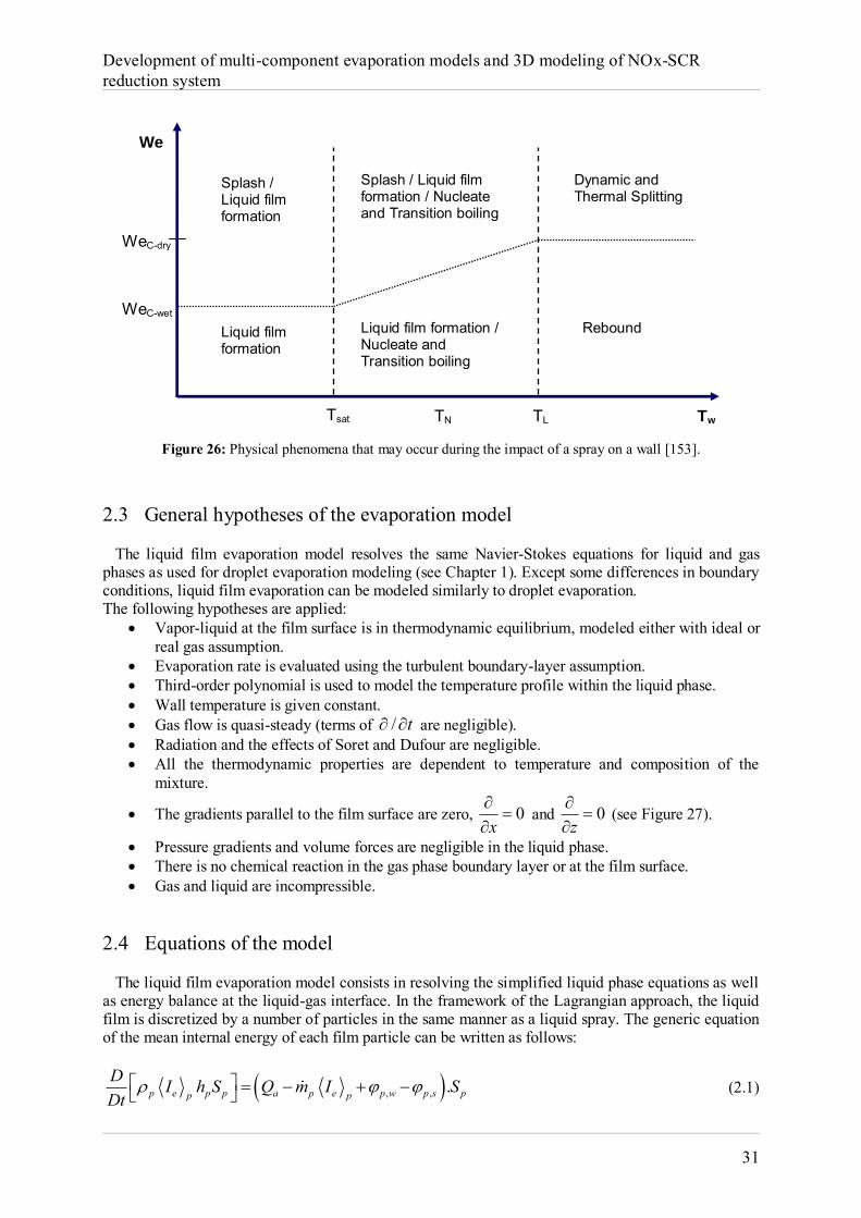
Development of multi-component evaporation models and 3D modeling of NOx-SCR reduction system
31
Figure 26: Physical phenomena that may occur during the impact of a spray on a wall [153].
2.3 General hypotheses of the evaporation model The liquid film evaporation model resolves the same Navier-Stokes equations for liquid and gas phases as used for droplet evaporation modeling (see Chapter 1). Except some differences in boundary conditions, liquid film evaporation can be modeled similarly to droplet evaporation. The following hypotheses are applied:
Vapor-liquid at the film surface is in thermodynamic equilibrium, modeled either with ideal or real gas assumption.
Evaporation rate is evaluated using the turbulent boundary-layer assumption. Third-order polynomial is used to model the temperature profile within the liquid phase. Wall temperature is given constant. Gas flow is quasi-steady (terms of / t are negligible). Radiation and the effects of Soret and Dufour are negligible. All the thermodynamic properties are dependent to temperature and composition of the
mixture.
The gradients parallel to the film surface are zero, 0x
and 0
z
(see Figure 27).
Pressure gradients and volume forces are negligible in the liquid phase. There is no chemical reaction in the gas phase boundary layer or at the film surface. Gas and liquid are incompressible.
2.4 Equations of the model The liquid film evaporation model consists in resolving the simplified liquid phase equations as well as energy balance at the liquid-gas interface. In the framework of the Lagrangian approach, the liquid film is discretized by a number of particles in the same manner as a liquid spray. The generic equation of the mean internal energy of each film particle can be written as follows:
, , .p e p p a p e p w p s pp p
D I h S Q m I SDt
(2.1)
Tw
Liquid film formation
Splash / Liquid film formation
Splash / Liquid film formation / Nucleate and Transition boiling
Dynamic and Thermal Splitting
Rebound Liquid film formation / Nucleate and Transition boiling
TL TN Tsat
We
WeC-dry
WeC-wet
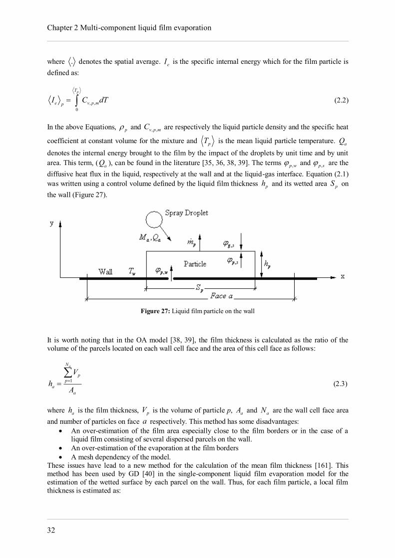
Chapter 2 Multi-component liquid film evaporation
32
where . denotes the spatial average. eI is the specific internal energy which for the film particle is defined as:
, ,0
pT
e v p mpI C dT (2.2)
In the above Equations, p and , ,v p mC are respectively the liquid particle density and the specific heat
coefficient at constant volume for the mixture and pT is the mean liquid particle temperature. aQ
denotes the internal energy brought to the film by the impact of the droplets by unit time and by unit area. This term, ( aQ ), can be found in the literature [35, 36, 38, 39]. The terms ,p w and ,p s are the diffusive heat flux in the liquid, respectively at the wall and at the liquid-gas interface. Equation (2.1) was written using a control volume defined by the liquid film thickness ph and its wetted area pS on the wall (Figure 27).
Figure 27: Liquid film particle on the wall
It is worth noting that in the OA model [38, 39], the film thickness is calculated as the ratio of the volume of the parcels located on each wall cell face and the area of this cell face as follows:
1
aN
pp
aa
Vh
A
(2.3)
where ah is the film thickness, pV is the volume of particle p, aA and aN are the wall cell face area and number of particles on face a respectively. This method has some disadvantages:
An over-estimation of the film area especially close to the film borders or in the case of a liquid film consisting of several dispersed parcels on the wall.
An over-estimation of the evaporation at the film borders A mesh dependency of the model.
These issues have lead to a new method for the calculation of the mean film thickness [161]. This method has been used by GD [40] in the single-component liquid film evaporation model for the estimation of the wetted surface by each parcel on the wall. Thus, for each film particle, a local film thickness is estimated as:
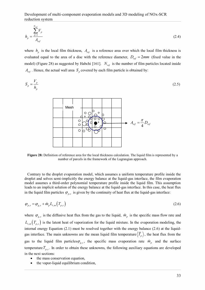
Development of multi-component evaporation models and 3D modeling of NOx-SCR reduction system
33
1
refN
pp
pref
Vh
A
(2.4)
where ph is the local film thickness, refA is a reference area over which the local film thickness is
evaluated equal to the area of a disc with the reference diameter, 2refD mm (fixed value in the
model) (Figure 28) as suggested by Habchi [161]. refN is the number of film particles located inside
refA . Hence, the actual wall area pS covered by each film particle is obtained by:
pp
p
VS
h (2.5)
Figure 28: Definition of reference area for the local thickness calculation. The liquid film is represented by a
number of parcels in the framework of the Lagrangian approach.
Contrary to the droplet evaporation model, which assumes a uniform temperature profile inside the droplet and solves semi-implicitly the energy balance at the liquid-gas interface, the film evaporation model assumes a third-order polynomial temperature profile inside the liquid film. This assumption leads to an implicit solution of the energy balance at the liquid-gas interface. In this case, the heat flux in the liquid film particles ,p s is given by the continuity of heat flux at the liquid-gas interface:
, , , ,p s g s p v m p sm L T (2.6) where ,g s is the diffusive heat flux from the gas to the liquid, pm is the specific mass flow rate and
, ,v m p sL T is the latent heat of vaporization for the liquid mixture. In the evaporation modeling, the internal energy Equation (2.1) must be resolved together with the energy balance (2.6) at the liquid-gas interface. The main unknowns are the mean liquid film temperature pT , the heat flux from the
gas to the liquid film particles ,g s , the specific mass evaporation rate pm and the surface
temperature ,p sT . In order to obtain these unknowns, the following auxiliary equations are developed in the next sections:
the mass conservation equation, the vapor-liquid equilibrium condition,
4ref refA D
Mesh
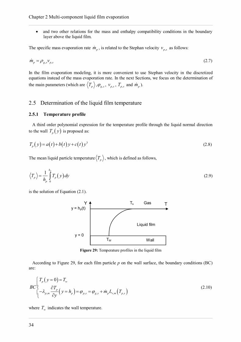
Chapter 2 Multi-component liquid film evaporation
34
and two other relations for the mass and enthalpy compatibility conditions in the boundary layer above the liquid film.
The specific mass evaporation rate pm , is related to the Stephan velocity ,p sv as follows:
, ,p g s p sm v (2.7) In the film evaporation modeling, it is more convenient to use Stephan velocity in the discretized equations instead of the mass evaporation rate. In the next Sections, we focus on the determination of the main parameters (which are pT , ,g s , ,p sv , ,p sT and pm ). 2.5 Determination of the liquid film temperature 2.5.1 Temperature profile A third order polynomial expression for the temperature profile through the liquid normal direction to the wall pT y is proposed as:
3pT y a t b t y c t y (2.8)
The mean liquid particle temperature pT , which is defined as follows,
0
1 ph
p pp
T T y dyh
(2.9)
is the solution of Equation (2.1).
Figure 29: Temperature profiles in the liquid film
According to Figure 29, for each film particle p on the wall surface, the boundary conditions (BC) are:
, , , , ,
0p w
pp m p p s g s p v m p s
T y TBC T
y h m L Ty
(2.10)
where wT indicates the wall temperature.
Y T y = hp(t)
y = 0 TW Wall
Liquid film
Gas Ts
Development of multi-component evaporation models and 3D modeling of NOx-SCR reduction system
35
Using the boundary conditions and the mean temperature of a particle film, one obtains the following expression for the temperature profile pT :
3
, ,
, ,
1 212 25 5
p s p p s pp w w p w p
p m p p m p
h hy yT y T T T T Th h
(2.11)
The temperature ,p sT at the surface of the particle film p could be obtained as:
,,
,
1 8 35
p s pp s p w
p m
hT T T
(2.12)
and the heat flux ,p w in the particle p on the wall:
,, ,
1 125
p mp w p s w p
p
T Th
(2.13)
2.5.2 Discretization of energy equation The mean liquid particle temperature is obtained by temporal discretization of Equation (2.1) in the following form:
1 1
1 1 1 1 1, ,
1n n n ne p e pp p n n n n n
a p e p w p sn pp
I h I hQ m I
t
(2.14)
where n
p is assumed to be constant. In IFP-C3D code, p is updated from the film particle
temperature at the beginning of each time step. In the above equation, 1nph is obtained by
discretization of mass conservation equation as follows:
111 .
nnpn n a
p p n np p
mMh h t
(2.15)
where aM indicates the mass source term by unit area of all the droplets that joint (or leave) the liquid film by impact on the face a where the particle p is located during the current time step (Figure 27). Substituting Equation (2.15) into Equation (2.14) gives:
1 11
1 1 1 1 1 1, ,
1n n n nne e pp p pn n n n n n a
a p e p w p s en n np pp p p
I I h mMQ m I It
(2.16)
In order to express Equation (2.16) as a function of the mean liquid temperature pT , the mean
internal energy e pI is written in the following form:

Chapter 2 Multi-component liquid film evaporation
36
0
0
, , , ,0
pTT
e v p m v p mpT
I C dT C dT (2.17)
In the above Equation, 0T has been chosen as the closest value to pT in such a way that:
0
, , , , 0 0
pT
v p m v p m pT
C dT C T T T and
0
, , 0 00
T
v p mC dT I T , where 0 0I T is known from the
table of internal energy. In this way, Equation (2.16) is simplified to the following Equation:
11
1, , , , 0 0 0
11 1
, ,1
n n nnp p pp pn n n na
v p m v p m pn pp
nn nap w p sn n
p p
T T h MC C T T I Tt
Q
(2.18)
Finally, the explicit equation which gives the mean particle temperature 1n
pT is:
1 1, ,
1
1 n npn p w p s impn
pnp
tot
E ET
C
(2.19)
where,
, ,
n np pn
pn v p m
T hE C
t
(2.20)
1 1, , 0 0 0
n n n na a v p m
imp np
Q M C T I TE
(2.21)
1
, ,
nnpn a
tot v p m np
hMC Ct
(2.22)
By substituting the expression of the heat flux (Equations (2.6) and (2.13)) into Equation (2.19), one obtains the following expression giving the temperature 1n
pT of the particle p at the time n+1 :
1
, 1 1 1, , ,1
11
,1
6 25
125
nw p m n n n
pn p v m p s g s impn np pn
p np m
tot n np p
TE m L T E
hT
Ch
(2.23)
where pnE , impE and totC are defined by Equations (2.20) to (2.22). Their value is known before the
resolution of Equation (2.23). Let recall here that in the above Equation, the gaseous heat flux 1,
ng s ,
Development of multi-component evaporation models and 3D modeling of NOx-SCR reduction system
37
surface temperature 1,
np sT and mass evaporation rate 1n
pm are the other unknowns which will be determined in the next Sections. 2.6 Determination of gaseous heat flux The gaseous heat flux is calculated from the temperature gradient at the interface of the liquid film. It is then necessary to determine the temperature profile in the gaseous boundary layer. In the framework of RANS (Reynolds Average Navier-Stokes) calculations, this is usually done using wall laws, which consist of resolving analytically the equations of the boundary layer on the surface of the wall or liquid film. In the present study, the multi-component mass, dynamic and thermal wall laws are obtained based on the wall laws of Desoutter et al. [51]. The single-component mass fraction wall law of Desoutter is generalized to multi-component wall law with the discrete fluid method. The thermal wall law is also modified by consideration of the new heat flux which takes into account the enthalpy diffusion of species in addition to conduction. These wall laws generalized for multi-component liquids are completely described in Appendix D and are summarized as follows:
:
: ln
lt eff
ult eff lt
lt
Ck
(2.24)
,
,
, ,, ,
: Pr
Pr1Pr 2 Pr: Pr ln
12
lt T eff l
s lt T l
u T t T tlt T eff l lt T
s lt T lt T
vC C C
vk
(2.25)
, , ,
, ,
, , , ,, ,
:
12: ln
12
lt m eff i l i
s lt m lt i
u Y t Y tlt m eff i lt i lt m
s lt m lt m
Sc
v ScC C Sc C ScSc
vk
(2.26)
where eff , eff and ,eff i are the dynamic, thermal and mass effective variables. ,lt ,lt T and ,lt m are the normalized distances from the liquid film surface to the laminar-turbulent transition, respectively, for the dynamic, thermal and the liquid mass fraction boundary layer. Their values are assumed to be the same as in the single-component wall laws. uC , TC and YC are the parameters obtained by comparing these wall laws with DNS results [40, 51] and k is the Karmann constant. Pr and Sc are the Prandtl and Schmidt numbers and subscripts t and l denote turbulent and laminar, respectively. The laminar Schmidt number of each component i is calculated in Appendix D. sv is the dimensionless Stephan velocity introduced as:
ss
vvu
(2.27)
Chapter 2 Multi-component liquid film evaporation
38
where u is the shear velocity. in Equations (2.24) to (2.26) is defined by [40, 51]:
,g s
g
y
(2.28)
where y is the non-dimensional coordinate, g is the laminar kinematic viscosity of the gas and subscript s denotes the film surface. Notice that in the limit of small evaporation rate and small gradients of density and viscosity, the wall laws given by Equations (2.24) to (2.26) reduce to the standard wall functions [162]. The heat flux ,g s is obtained using the enthalpy compatibility condition:
0
0
1
1
m
m
L
g pm
Lm
g pm
y C y T y dyL
Ty C y dy
L
(2.29)
where m
X and mL denote the RANS mean value of a variable X in the wall cell and the size of the cell in the normal direction to the wall. In this case, the thermal wall law is implemented by resolving Equation (2.29) inside the grid cell adjacent to the wall. The resolution of Equation (2.29) gives the gas heat flux ,g s at the film surface, as shown below. Using Equations (11.60), (11.57), (11.63) and (11.66) gives the explicit profile of gas temperature in the boundary layer:
2 Pr,
, 1 , T tCg sp s s
ct s
T y T HgT y vr v
(2.30)
with
, ,ct g s p mr C u (2.31)
,
,
, ,, ,
Pr, 1
Pr1Pr 2 Pr, 1 Pr ln
12
s ls lt T
s lt T l
s u T t T ts l lt T lt T
s lt T lt T
vHgT y v ifhTden
vv C C CHgT y v if
vhTden k
(2.32)
and
2 PrT t ThTden C P (2.33)
Development of multi-component evaporation models and 3D modeling of NOx-SCR reduction system
39
where sv is the dimensionless Stephan velocity as a function of shear velocity u (Equation (11.12))
and is defined by Equation (11.61). TP is defined by:
,0
1 mLg
T effeff g s
P dTT
(2.34)
where effT is the effective thermal parameter [51]. This function is used to simplify the LnKc model (Equation (11.63)) as follows:
eff T effP T (2.35)
Substituting the expression of temperature (Equation (2.30)) in Equation (2.29), one obtains the following expression:
2 Pr,,
0
0
1 1 ,
1
mT t
m
LCg s
g p p s sm ct s
Lm
g pm
y C y T HgT y v dyL r v
Ty C y dy
L
(2.36)
After simplifications, the following expression for ,g s as a function of the film surface temperature
,p sT and the dimensionless Stephan velocity sv is obtained:
, ,rcp
g s ct s p smerg s
Ir v T T
I v
(2.37)
where
0
1 mL
rcp g pm
I y C y dyL
(2.38)
2 Pr
0
1 1 ,m
T tL
C
erg s g p sm
I v y C y HgT y v dyL
(2.39)
It is worth noting that the profiles of density g y and heat capacity in the gas pC y in Equations
(2.51) and (2.37), are calculated through the temperature profile T y (Equation (2.30)) and mass
fraction of liquid ,i gY y (Equations (2.47)). These profiles are evaluated explicitly. The discretized form of Equation (2.37) is then written in the following form:
11 11 1 1
, ,1
nn nrcpn n n
g s ct s p sn merg s
Ir v T T
I v
(2.40)
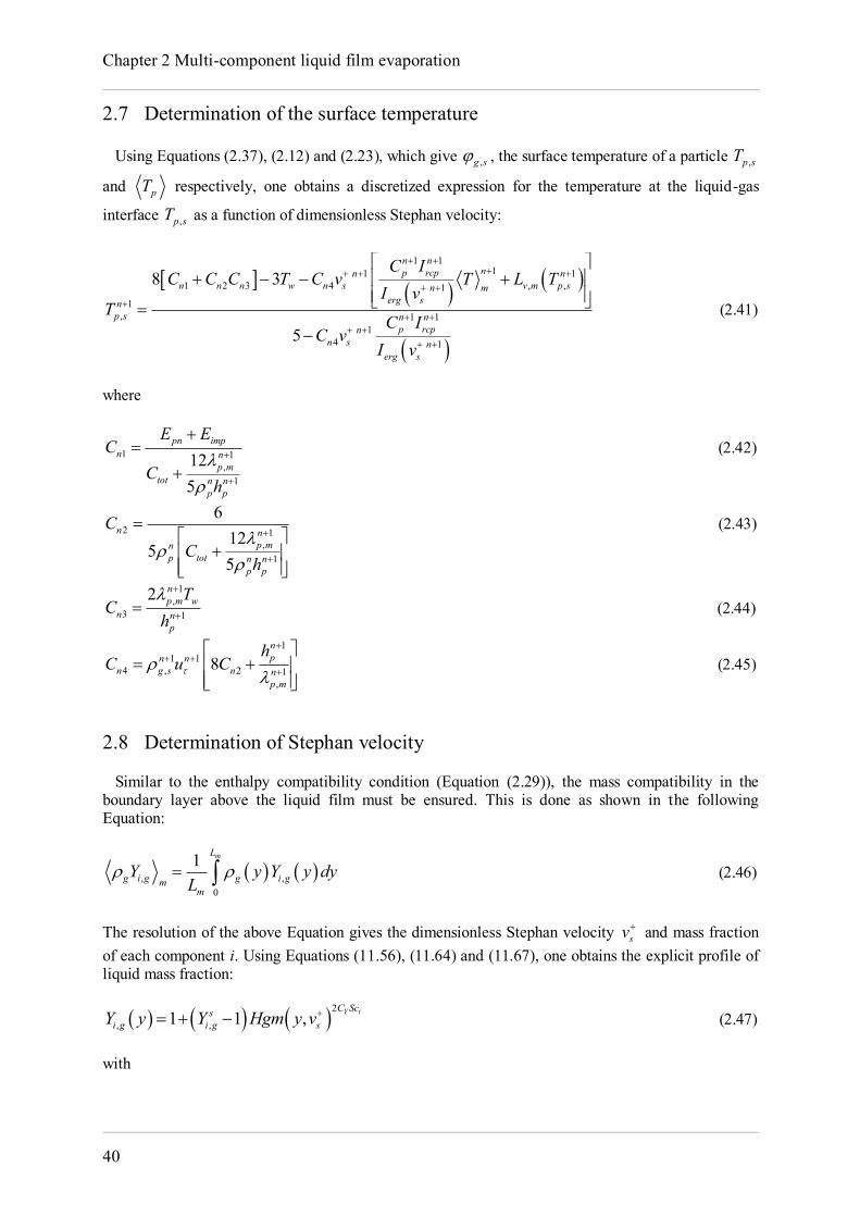
Chapter 2 Multi-component liquid film evaporation
40
2.7 Determination of the surface temperature Using Equations (2.37), (2.12) and (2.23), which give ,g s , the surface temperature of a particle ,p sT
and pT respectively, one obtains a discretized expression for the temperature at the liquid-gas
interface ,p sT as a function of dimensionless Stephan velocity:
1 11 1 1
1 2 3 4 , , 11
, 1 1 1
4 1
8 3
5
n nnp rcpn n
n n n w n s v m p sn merg sn
p s n np rcpn
n s nerg s
C IC C C T C v T L T
I vT
C IC v
I v
(2.41)
where
1 1,
1
125
pn impn n
p mtot n n
p p
E EC
Ch
(2.42)
2 1,
1
612
55
n np mn
p tot n np p
CC
h
(2.43)
1,
3 1
2 np m w
n np
TC
h
(2.44)
11 1
4 , 2 1,
8npn n
n g s n np m
hC u C
(2.45)
2.8 Determination of Stephan velocity Similar to the enthalpy compatibility condition (Equation (2.29)), the mass compatibility in the boundary layer above the liquid film must be ensured. This is done as shown in the following Equation:
, ,0
1 mL
g i g g i gmm
Y y Y y dyL
(2.46)
The resolution of the above Equation gives the dimensionless Stephan velocity sv and mass fraction of each component i. Using Equations (11.56), (11.64) and (11.67), one obtains the explicit profile of liquid mass fraction:
2
, ,1 1 , Y tC Scsi g i g sY y Y Hgm y v (2.47)
with
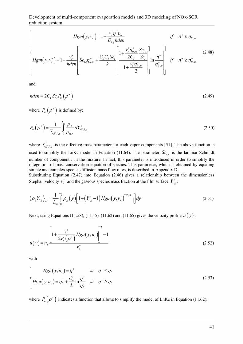
Development of multi-component evaporation models and 3D modeling of NOx-SCR reduction system
41
,,
, ,
, , ,, ,
, 1
12, 1 ln
12
s ms lt m
i g
s lt m l i
s u Y t Y ts l i lt m lt m
s lt m lt m
vHgm y v ifD hden
v Scv C C Sc C ScHgm y v Sc if
vhden k
(2.48)
and
2 Y t mhden C Sc P (2.49) where mP is defined by:
, ,, , ,0
1 mLg
m eff i geff i g g s
P dYY
(2.50)
where , ,eff i gY is the effective mass parameter for each vapor components [51]. The above function is
used to simplify the LnKc model in Equation (11.64). The parameter ,l iSc is the laminar Schmidt number of component i in the mixture. In fact, this parameter is introduced in order to simplify the integration of mass conservation equation of species. This parameter, which is obtained by equating simple and complex species diffusion mass flow rates, is described in Appendix D. Substituting Equation (2.47) into Equation (2.46) gives a relationship between the dimensionless Stephan velocity sv and the gaseous species mass fraction at the film surface ,
si gY :
2
, ,0
1 1 1 ,m
Y tL
C Scsg i g g i g sm
m
Y y Y Hgm y v dyL
(2.51)
Next, using Equations (11.58), (11.55), (11.62) and (11.65) gives the velocity profile u y :
2
1 , 12
s
u
s
v Hgu y uP
u y uv
(2.52)
with
,
, ln
lt
ult lt
lt
Hgu y u siCHgu y u sik
(2.53)
where uP indicates a function that allows to simplify the model of LnKc in Equation (11.62):
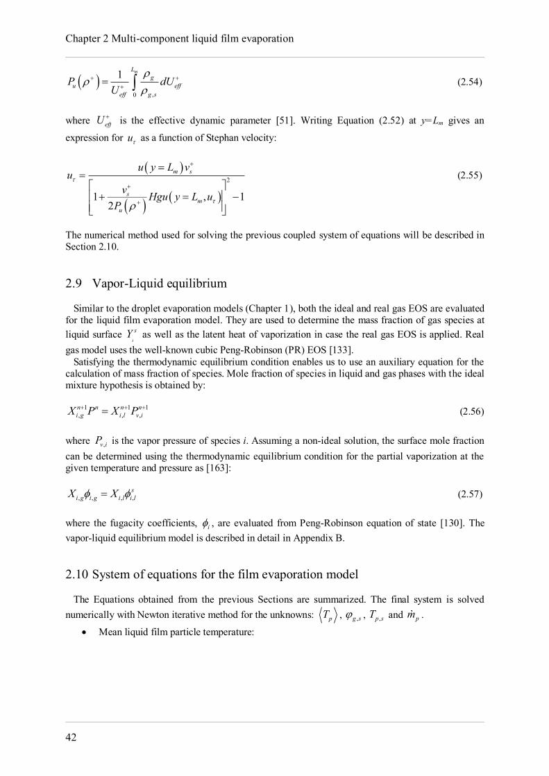
Chapter 2 Multi-component liquid film evaporation
42
,0
1 mLg
u effeff g s
P dUU
(2.54)
where effU is the effective dynamic parameter [51]. Writing Equation (2.52) at y=Lm gives an
expression for u as a function of Stephan velocity:
2
1 , 12
m s
sm
u
u y L vu
v Hgu y L uP
(2.55)
The numerical method used for solving the previous coupled system of equations will be described in Section 2.10. 2.9 Vapor-Liquid equilibrium Similar to the droplet evaporation models (Chapter 1), both the ideal and real gas EOS are evaluated for the liquid film evaporation model. They are used to determine the mass fraction of gas species at liquid surface
i
sY as well as the latent heat of vaporization in case the real gas EOS is applied. Real gas model uses the well-known cubic Peng-Robinson (PR) EOS [133]. Satisfying the thermodynamic equilibrium condition enables us to use an auxiliary equation for the calculation of mass fraction of species. Mole fraction of species in liquid and gas phases with the ideal mixture hypothesis is obtained by:
1 1 1, , ,n n n ni g i l v iX P X P (2.56)
where ,v iP is the vapor pressure of species i. Assuming a non-ideal solution, the surface mole fraction can be determined using the thermodynamic equilibrium condition for the partial vaporization at the given temperature and pressure as [163]:
, , , ,s
i g i g i l i lX X (2.57) where the fugacity coefficients, i , are evaluated from Peng-Robinson equation of state [130]. The vapor-liquid equilibrium model is described in detail in Appendix B. 2.10 System of equations for the film evaporation model The Equations obtained from the previous Sections are summarized. The final system is solved numerically with Newton iterative method for the unknowns: pT , ,g s , ,p sT and pm .
Mean liquid film particle temperature:
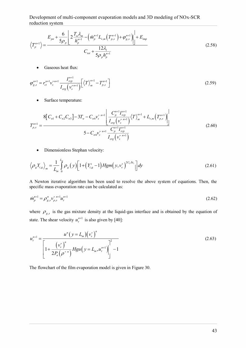
Development of multi-component evaporation models and 3D modeling of NOx-SCR reduction system
43
1 1 1, , ,1
1
1
6 25
125
n n nw mpn p v m p s g s impn
p pnp
ltot n
p p
TE m L T Eh
TC
h
(2.58)
Gaseous heat flux:
111 1 1 1
, ,1
nnrcpn n n n
g s ct s p smnerg s
Ir v T T
I v
(2.59)
Surface temperature:
1 11 1 1
1 2 3 4 , , 11
, 1 1 1
4 1
8 3
5
n nnp rcpn n
n n n w n s v m p sn merg sn
p s n np rcpn
n s nerg s
C IC C C T C v T L T
I vT
C IC v
I v
(2.60)
Dimensionless Stephan velocity:
2
, ,0
1 1 1 ,m
Y tL
C Scsg i g g i g sm
m
Y y Y Hgm y v dyL
(2.61)
A Newton iterative algorithm has been used to resolve the above system of equations. Then, the specific mass evaporation rate can be calculated as:
1 1 1, ,
n n n np g s p sm v u (2.62)
where ,g s is the gas mixture density at the liquid-gas interface and is obtained by the equation of
state. The shear velocity 1nu is also given by [40]:
12
1 1 , 1
2
nnm sn
n
s nmn
u
u y L vu
vHgu y L u
P
(2.63)
The flowchart of the film evaporation model is given in Figure 30.
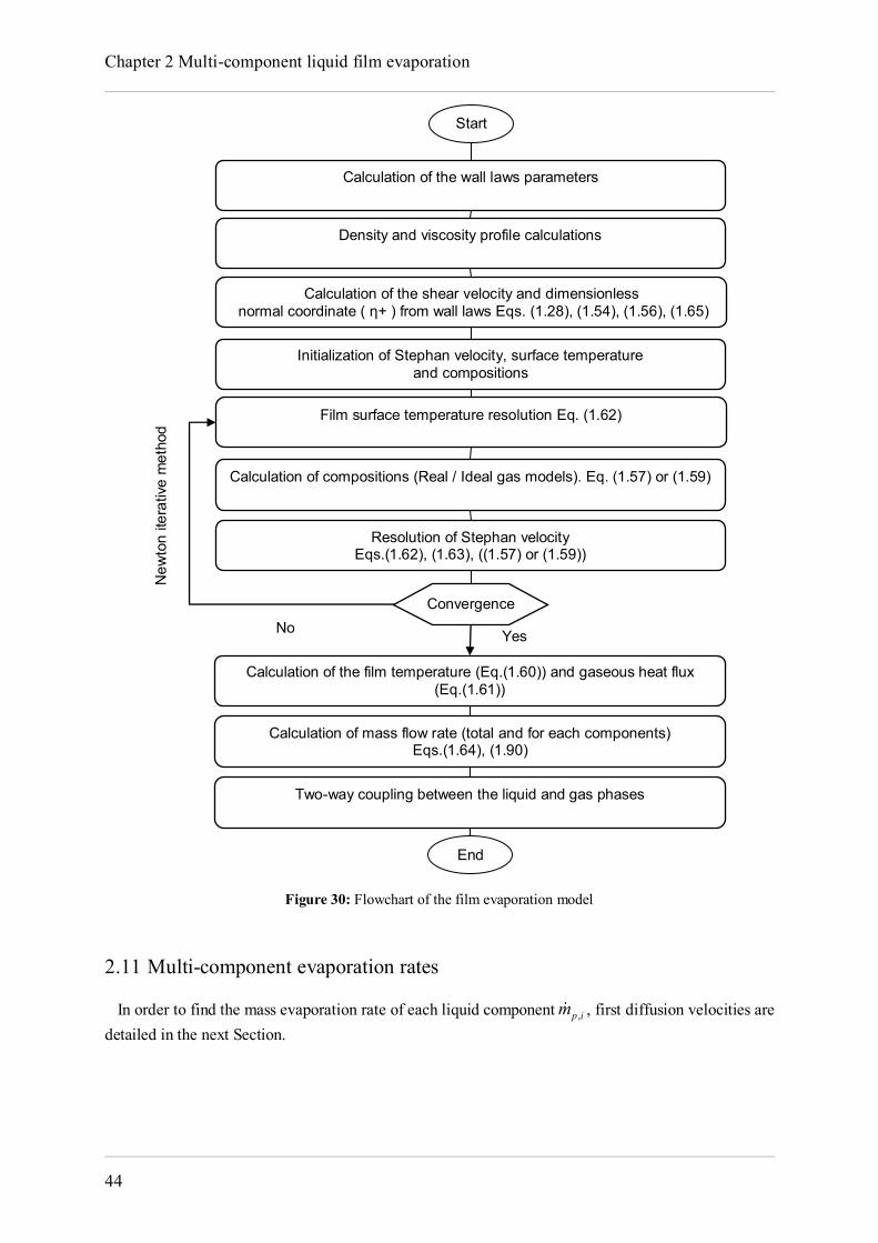
Chapter 2 Multi-component liquid film evaporation
44
Figure 30: Flowchart of the film evaporation model
2.11 Multi-component evaporation rates In order to find the mass evaporation rate of each liquid component ,p im , first diffusion velocities are detailed in the next Section.
Initialization of Stephan velocity, surface temperature and compositions
Film surface temperature resolution Eq. (1.62)
Calculation of compositions (Real / Ideal gas models). Eq. (1.57) or (1.59)
Resolution of Stephan velocity Eqs.(1.62), (1.63), ((1.57) or (1.59))
Calculation of mass flow rate (total and for each components) Eqs.(1.64), (1.90)
Convergence
Yes No
Calculation of the wall laws parameters
Calculation of the shear velocity and dimensionless normal coordinate ( η+ ) from wall laws Eqs. (1.28), (1.54), (1.56), (1.65)
Density and viscosity profile calculations
Calculation of the film temperature (Eq.(1.60)) and gaseous heat flux (Eq.(1.61))
Two-way coupling between the liquid and gas phases
New
ton
itera
tive
met
hod
Start
End
Development of multi-component evaporation models and 3D modeling of NOx-SCR reduction system
45
2.11.1 Diffusion velocities As mentioned earlier for droplet evaporation model, the diffusion velocity is used for the calculation of mass evaporation rate of each liquid film component. In the mass conservation equation, the correction velocity is evaluated to ensure global mass conservation. Similar to droplets, the correction velocity is obtained as:
1 1 or u
N Nc ck k k k
k kk k k
W X D Xu D YW y X y
(2.64)
and, at the liquid-gas interface, the diffusion velocity will be:
1. .
s sNs s c sk kk k s s
k s s
D X D Xu V u YX y X y
(2.65)
2.11.2 Calculation of film evaporation rate for each component At the liquid-gas interface one has:
11
Ns
kk
Y
or 1 1 1
1G LN NN
s s sj k i
j k iY Y Y
or 1 1
1G LN N
s sk i
k iY Y
(2.66)
where GN is the number of gaseous species. For the total evaporated mass of liquid film, one has:
, , , , , , , ,1 1 1
L L LN N Ns c s s s
g s s g s s i g g s i g g s i g i gi i i
m v v Y u Y Y V
(2.67)
or by introducing the mass fraction of gas species 1
GNs
kk
Y
:
, ,1 1
G LN Ns s
g s s g s s k ik i
m v v Y Y
. (2.68)
By equating the equations of mass evaporation rate (Equations (2.67) and (2.68)) and assuming that the simple diffusion velocity is negligible compared to the correction velocity, one has:
, , , , ,1 1 1 1 1
G L L L LN N N N Ns s s c s s s
g s s k g s s i g s s i g s i g s ik i i i i
v Y v Y v Y u Y V Y
. (2.69)
The simplification of the above Equation leads to:
1 1 1
G L LN N Ns c s s s
s k i ik i i
v Y u Y V Y
(2.70)
or
Chapter 2 Multi-component liquid film evaporation
46
1 1 11
L L LN N Ns c s s s
s i i ii i i
v Y u Y V Y
(2.71)
or even
1 1
1L LN N
s c s ss i i
i iv Y u V Y
. (2.72)
Finally,
1
1
1L
L
Ns
s iic s
Ns
ii
v Yu V
Y
. (2.73)
Thus, for each component i of the film, one can write the following relation for the specific mass flow rate of each liquid film particle component:
1, , , ,
1
1L
L
Ns
s iis c s s s
p i g s s i g s i g s i s Ns
ii
v Ym v Y u V Y Y v
Y
(2.74)
And finally:
,
1
L
si
p i p Ns
ii
Ym mY
(2.75)
The above specific film mass evaporation rates are obtained similar to the droplet mass evaporation rate. The present multi-component film evaporation model is implemented in IFP-C3D code [139] and used to simulate the following test cases. A brief description of IFP-C3D code is given in Appendix E. 2.12 Liquid film evaporation test cases In order to investigate the multi-component liquid film evaporation model developed in this work, two test cases are studied in this section: The turbulent channel flow and the spray-film interaction test cases. These test cases have been built in order to investigate numerically the new model in situations where a gas turbulent flow dominates (i.e. similar to the operating conditions in internal combustion engines for example). In these conditions, very few experiments or numerical investigations exist, and comparison with experimental data is not possible. However, a comprehensive comparison between three-component fuel and single pseudo-component fuel evaporation model (obtained by the lumping of the three-components) will be presented. The second “spray-film interaction” test case is the simulation of experiments recently obtained at IFP Energies nouvelles [74, 164]. These experiments consist in the measurement of the film thickness which was formed by the injection and impingement of a hollow cone spray on a flat plate.
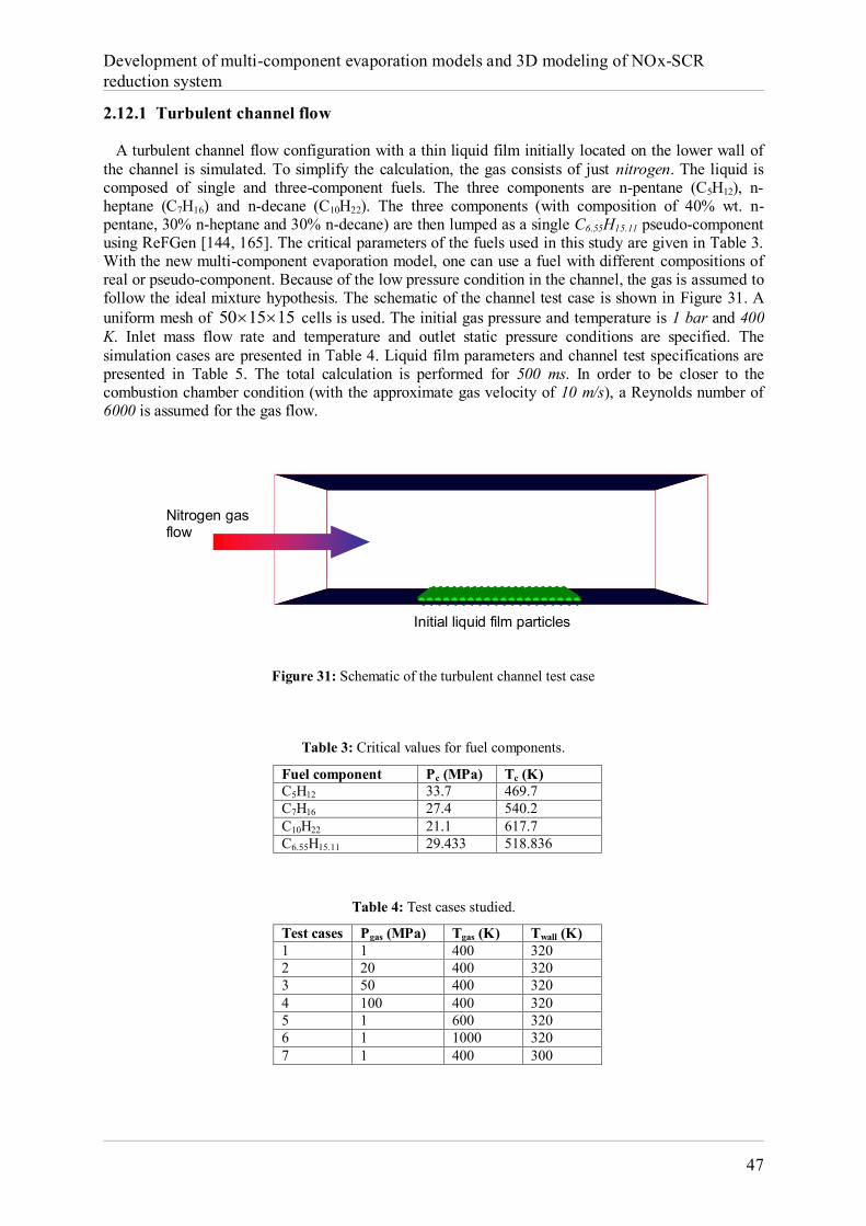
Development of multi-component evaporation models and 3D modeling of NOx-SCR reduction system
47
2.12.1 Turbulent channel flow A turbulent channel flow configuration with a thin liquid film initially located on the lower wall of the channel is simulated. To simplify the calculation, the gas consists of just nitrogen. The liquid is composed of single and three-component fuels. The three components are n-pentane (C5H12), n-heptane (C7H16) and n-decane (C10H22). The three components (with composition of 40% wt. n-pentane, 30% n-heptane and 30% n-decane) are then lumped as a single C6.55H15.11 pseudo-component using ReFGen [144, 165]. The critical parameters of the fuels used in this study are given in Table 3. With the new multi-component evaporation model, one can use a fuel with different compositions of real or pseudo-component. Because of the low pressure condition in the channel, the gas is assumed to follow the ideal mixture hypothesis. The schematic of the channel test case is shown in Figure 31. A uniform mesh of 50 15 15 cells is used. The initial gas pressure and temperature is 1 bar and 400 K. Inlet mass flow rate and temperature and outlet static pressure conditions are specified. The simulation cases are presented in Table 4. Liquid film parameters and channel test specifications are presented in Table 5. The total calculation is performed for 500 ms. In order to be closer to the combustion chamber condition (with the approximate gas velocity of 10 m/s), a Reynolds number of 6000 is assumed for the gas flow.
Figure 31: Schematic of the turbulent channel test case
Table 3: Critical values for fuel components. Fuel component Pc (MPa) Tc (K) C5H12 33.7 469.7 C7H16 27.4 540.2 C10H22 21.1 617.7 C6.55H15.11 29.433 518.836
Table 4: Test cases studied.
Test cases Pgas (MPa) Tgas (K) Twall (K) 1 1 400 320 2 20 400 320 3 50 400 320 4 100 400 320 5 1 600 320 6 1 1000 320 7 1 400 300
Nitrogen gas flow
Initial liquid film particles
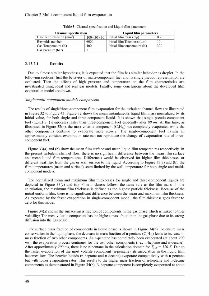
Chapter 2 Multi-component liquid film evaporation
48
Table 5: Channel specification and Liquid film parameters
Channel specification Liquid film parameters Channel dimension (mm3) 100 30 30 Initial film mass (mg) 0.7 Reynolds number 6000 Initial film Thickness (µm) 10 Gas Temperature (K) 400 Initial film temperature (K) 300 Gas Pressure (bar) 1
2.12.2.1 Results Due to almost similar hypotheses, it is expected that the film has similar behavior as droplet. In the following sections, first the behavior of multi-component fuel and its single pseudo representation are evaluated. Then the effects of high pressure and temperature on the film characteristics are investigated using ideal and real gas models. Finally, some conclusions about the developed film evaporation model are drawn. Single/multi-component models comparison The results of single/three-component film evaporation for the turbulent channel flow are illustrated in Figure 32 to Figure 43. Figure 32 shows the mean instantaneous liquid film mass normalized by its initial value, for both single and three-component liquid. It is shown that single pseudo-component fuel (C6.55H15.11) evaporates faster than three-component fuel especially after 80 ms. At this time, as illustrated in Figure 32(b), the most volatile component (C5H12) has completely evaporated while the other components continue to evaporate more slowly. The single-component fuel having an approximately constant evaporation rate can not reproduce the change of evaporation rate of three-component fuel. Figure 33(a) and (b) show the mean film surface and mean liquid film temperatures respectively. In the present turbulent channel flow, there is no significant difference between the mean film surface and mean liquid film temperatures. Differences would be observed for higher film thicknesses or different heat flux from the gas or wall surface to the liquid. According to Figure 33(a) and (b), the film temperatures (mean and surface) seem limited by the wall temperature for both single and multi-component models. The normalized mean and maximum film thicknesses for single and three-component liquids are depicted in Figure 33(c) and (d). Film thickness follows the same rule as the film mass. In the calculation, the maximum film thickness is defined as the highest particle thickness. Because of the initial uniform film, there is no significant difference between the mean and maximum film thickness. As expected by the faster evaporation in single-component model, the film thickness goes faster to zero for this model. Figure 34(a) shows the surface mass fraction of components in the gas phase which is linked to thier volatility: The most volatile component has the highest mass fraction in the gas phase due to its strong diffusion into the gas phase. The surface mass fraction of components in liquid phase is shown in Figure 34(b). To ensure mass conservation in the liquid phase, the decrease in mass fraction of n-pentane (C5H12) leads to increase in mass fraction of two other components. As n-pentane has completely been evaporated (at about 200 ms), the evaporation process continues for the two other components (i.e., n-heptane and n-decane). After approximately 200 ms, there is no n-pentane in the calculation domain for Twall = 320 K. Due to the faster evaporation of the most volatile component (n-pentane), its association in the liquid film becomes low. The heavier liquids (n-heptane and n-decane) evaporate competitively with n-pentane but with lower evaporation rates. This results to the higher mass fraction of n-heptane and n-decane components as demonstrated in Figure 34(b). N-heptane component is completely evaporated at about
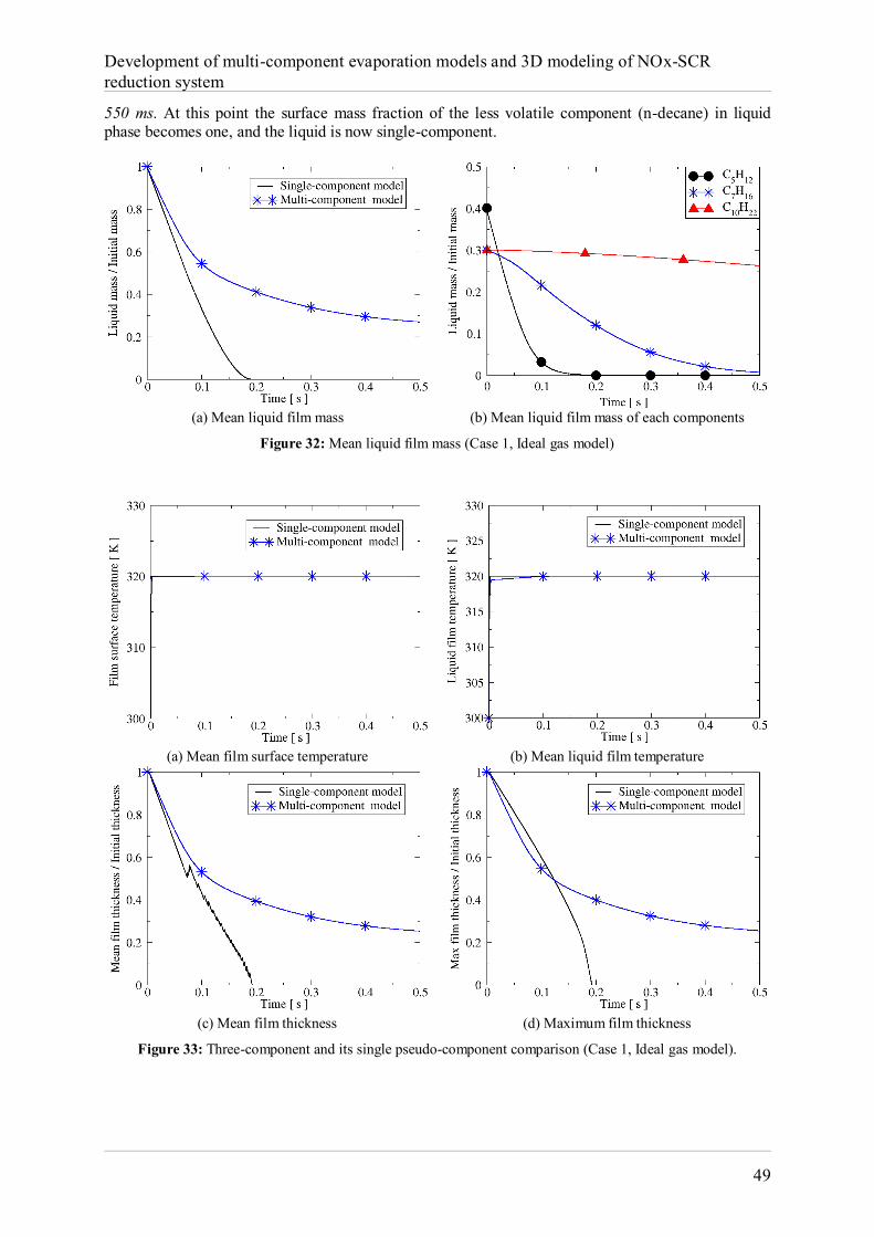
Development of multi-component evaporation models and 3D modeling of NOx-SCR reduction system
49
550 ms. At this point the surface mass fraction of the less volatile component (n-decane) in liquid phase becomes one, and the liquid is now single-component.
(a) Mean liquid film mass (b) Mean liquid film mass of each components
Figure 32: Mean liquid film mass (Case 1, Ideal gas model)
(a) Mean film surface temperature (b) Mean liquid film temperature
(c) Mean film thickness (d) Maximum film thickness
Figure 33: Three-component and its single pseudo-component comparison (Case 1, Ideal gas model).
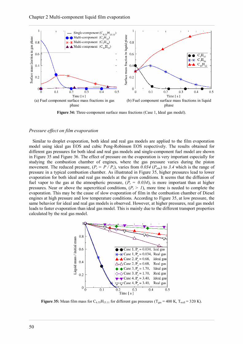
Chapter 2 Multi-component liquid film evaporation
50
(a) Fuel component surface mass fractions in gas
phase (b) Fuel component surface mass fractions in liquid
phase
Figure 34: Three-component surface mass fractions (Case 1, Ideal gas model).
Pressure effect on film evaporation Similar to droplet evaporation, both ideal and real gas models are applied to the film evaporation model using ideal gas EOS and cubic Peng-Robinson EOS respectively. The results obtained for different gas pressures for both ideal and real gas models and single-component fuel model are shown in Figure 35 and Figure 36. The effect of pressure on the evaporation is very important especially for studying the combustion chamber of engines, where the gas pressure varies during the piston movement. The reduced pressure, (Pr = P / Pc), varies from 0.034 (Patm) to 3.4 which is the range of pressure in a typical combustion chamber. As illustrated in Figure 35, higher pressures lead to lower evaporation for both ideal and real gas models at the given conditions. It seems that the diffusion of fuel vapor to the gas at the atmospheric pressure, (Pr = 0.034), is more important than at higher pressures. Near or above the supercritical conditions, (Pr > 1), more time is needed to complete the evaporation. This may be the cause of slow evaporation of film in the combustion chamber of Diesel engines at high pressure and low temperature conditions. According to Figure 35, at low pressure, the same behavior for ideal and real gas models is observed. However, at higher pressures, real gas model leads to faster evaporation than ideal gas model. This is mainly due to the different transport properties calculated by the real gas model.
Figure 35: Mean film mass for C6.55H15.11 for different gas pressures (Tgas = 400 K, Twall = 320 K).
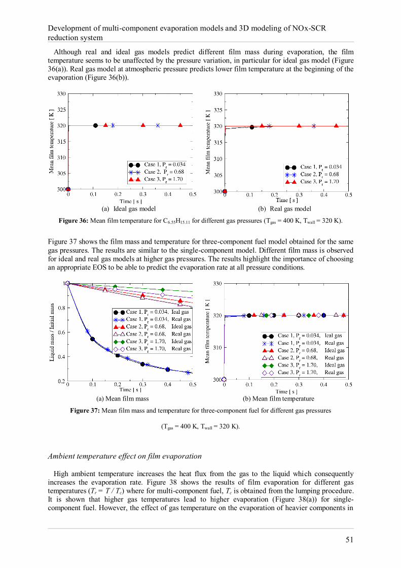
Development of multi-component evaporation models and 3D modeling of NOx-SCR reduction system
51
Although real and ideal gas models predict different film mass during evaporation, the film temperature seems to be unaffected by the pressure variation, in particular for ideal gas model (Figure 36(a)). Real gas model at atmospheric pressure predicts lower film temperature at the beginning of the evaporation (Figure 36(b)).
(a) Ideal gas model (b) Real gas model
Figure 36: Mean film temperature for C6.55H15.11 for different gas pressures (Tgas = 400 K, Twall = 320 K).
Figure 37 shows the film mass and temperature for three-component fuel model obtained for the same gas pressures. The results are similar to the single-component model. Different film mass is observed for ideal and real gas models at higher gas pressures. The results highlight the importance of choosing an appropriate EOS to be able to predict the evaporation rate at all pressure conditions.
(a) Mean film mass (b) Mean film temperature
Figure 37: Mean film mass and temperature for three-component fuel for different gas pressures
(Tgas = 400 K, Twall = 320 K).
Ambient temperature effect on film evaporation High ambient temperature increases the heat flux from the gas to the liquid which consequently increases the evaporation rate. Figure 38 shows the results of film evaporation for different gas temperatures (Tr = T / Tc) where for multi-component fuel, Tc is obtained from the lumping procedure. It is shown that higher gas temperatures lead to higher evaporation (Figure 38(a)) for single-component fuel. However, the effect of gas temperature on the evaporation of heavier components in
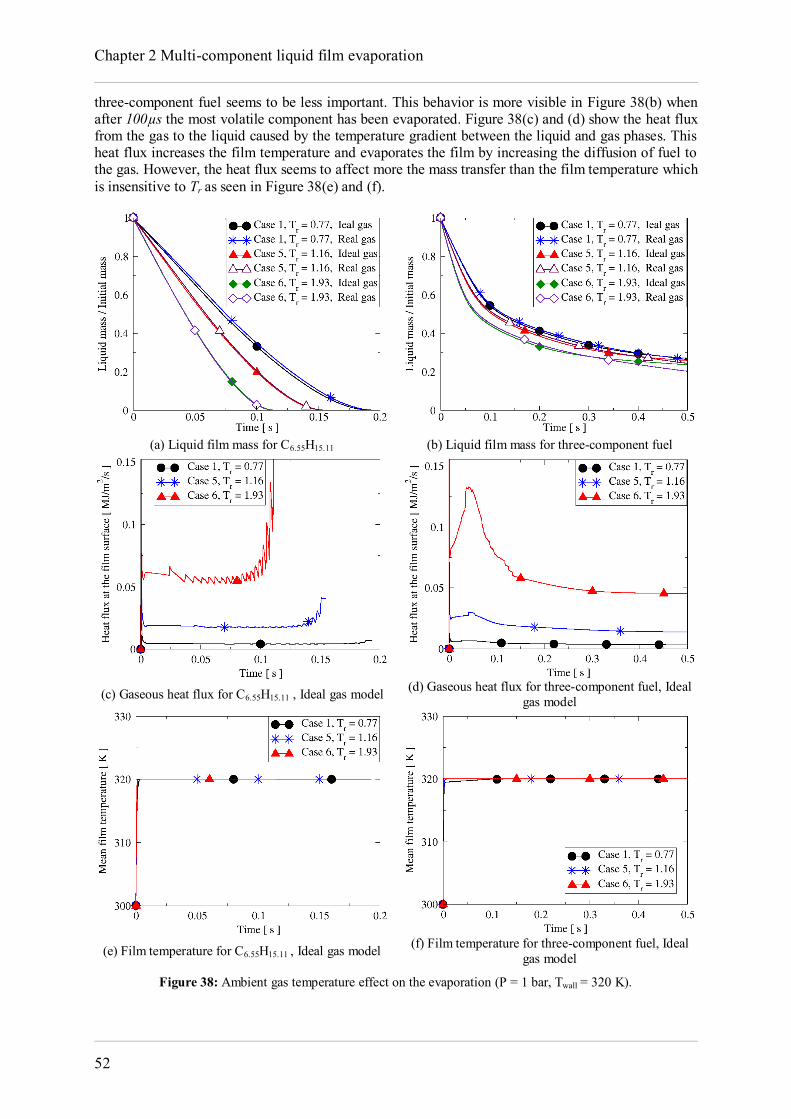
Chapter 2 Multi-component liquid film evaporation
52
three-component fuel seems to be less important. This behavior is more visible in Figure 38(b) when after 100µs the most volatile component has been evaporated. Figure 38(c) and (d) show the heat flux from the gas to the liquid caused by the temperature gradient between the liquid and gas phases. This heat flux increases the film temperature and evaporates the film by increasing the diffusion of fuel to the gas. However, the heat flux seems to affect more the mass transfer than the film temperature which is insensitive to Tr as seen in Figure 38(e) and (f).
(a) Liquid film mass for C6.55H15.11 (b) Liquid film mass for three-component fuel
(c) Gaseous heat flux for C6.55H15.11 , Ideal gas model (d) Gaseous heat flux for three-component fuel, Ideal
gas model
(e) Film temperature for C6.55H15.11 , Ideal gas model (f) Film temperature for three-component fuel, Ideal
gas model
Figure 38: Ambient gas temperature effect on the evaporation (P = 1 bar, Twall = 320 K).
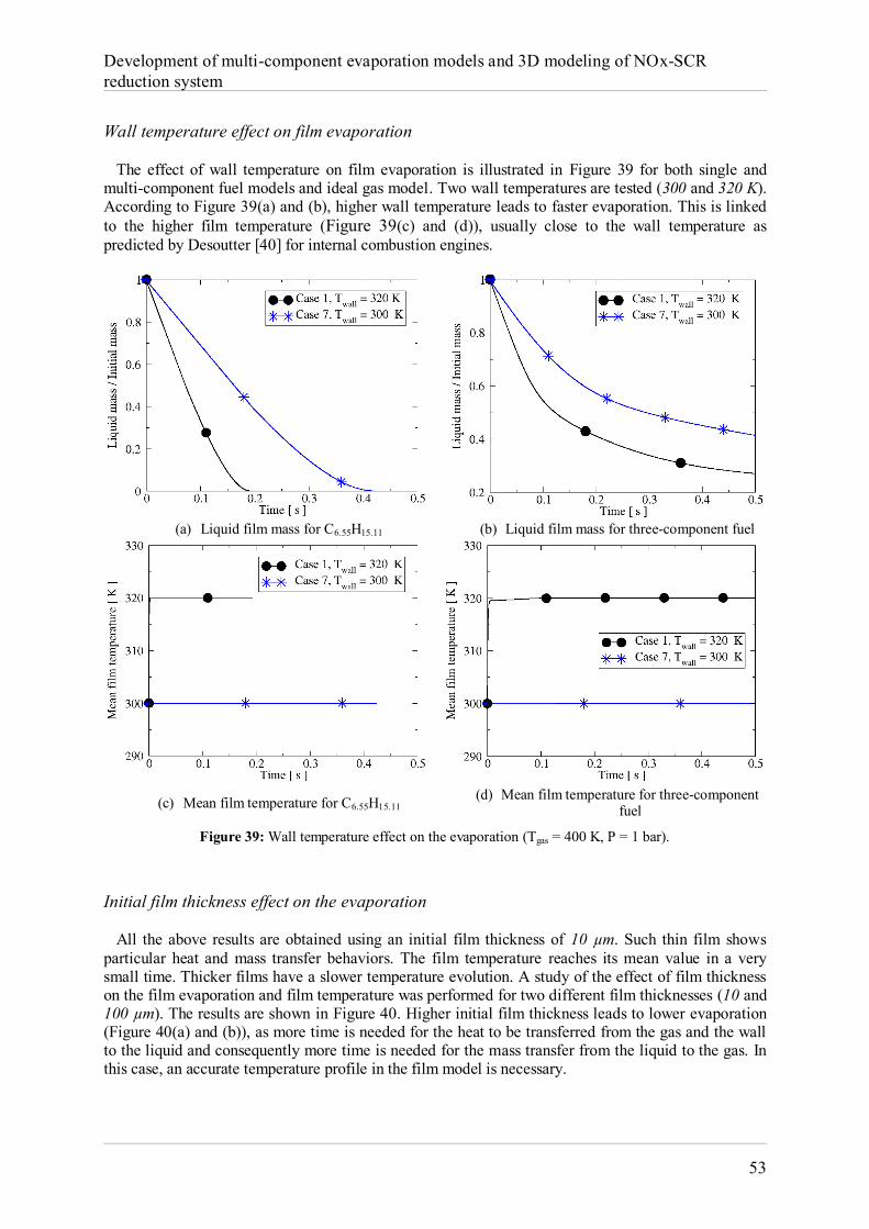
Development of multi-component evaporation models and 3D modeling of NOx-SCR reduction system
53
Wall temperature effect on film evaporation The effect of wall temperature on film evaporation is illustrated in Figure 39 for both single and multi-component fuel models and ideal gas model. Two wall temperatures are tested (300 and 320 K). According to Figure 39(a) and (b), higher wall temperature leads to faster evaporation. This is linked to the higher film temperature (Figure 39(c) and (d)), usually close to the wall temperature as predicted by Desoutter [40] for internal combustion engines.
(a) Liquid film mass for C6.55H15.11 (b) Liquid film mass for three-component fuel
(c) Mean film temperature for C6.55H15.11
(d) Mean film temperature for three-component fuel
Figure 39: Wall temperature effect on the evaporation (Tgas = 400 K, P = 1 bar).
Initial film thickness effect on the evaporation All the above results are obtained using an initial film thickness of 10 µm. Such thin film shows particular heat and mass transfer behaviors. The film temperature reaches its mean value in a very small time. Thicker films have a slower temperature evolution. A study of the effect of film thickness on the film evaporation and film temperature was performed for two different film thicknesses (10 and 100 µm). The results are shown in Figure 40. Higher initial film thickness leads to lower evaporation (Figure 40(a) and (b)), as more time is needed for the heat to be transferred from the gas and the wall to the liquid and consequently more time is needed for the mass transfer from the liquid to the gas. In this case, an accurate temperature profile in the film model is necessary.
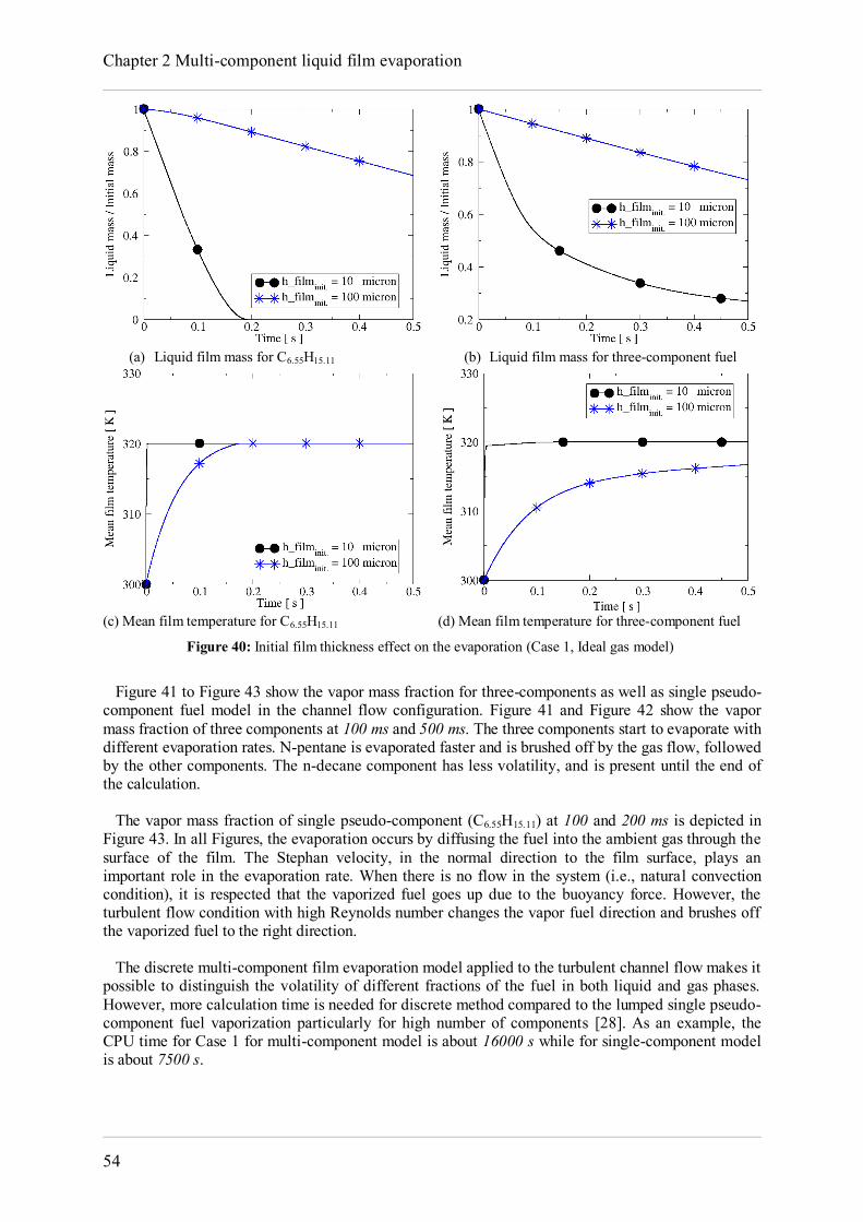
Chapter 2 Multi-component liquid film evaporation
54
(a) Liquid film mass for C6.55H15.11 (b) Liquid film mass for three-component fuel
(c) Mean film temperature for C6.55H15.11 (d) Mean film temperature for three-component fuel
Figure 40: Initial film thickness effect on the evaporation (Case 1, Ideal gas model)
Figure 41 to Figure 43 show the vapor mass fraction for three-components as well as single pseudo-component fuel model in the channel flow configuration. Figure 41 and Figure 42 show the vapor mass fraction of three components at 100 ms and 500 ms. The three components start to evaporate with different evaporation rates. N-pentane is evaporated faster and is brushed off by the gas flow, followed by the other components. The n-decane component has less volatility, and is present until the end of the calculation. The vapor mass fraction of single pseudo-component (C6.55H15.11) at 100 and 200 ms is depicted in Figure 43. In all Figures, the evaporation occurs by diffusing the fuel into the ambient gas through the surface of the film. The Stephan velocity, in the normal direction to the film surface, plays an important role in the evaporation rate. When there is no flow in the system (i.e., natural convection condition), it is respected that the vaporized fuel goes up due to the buoyancy force. However, the turbulent flow condition with high Reynolds number changes the vapor fuel direction and brushes off the vaporized fuel to the right direction. The discrete multi-component film evaporation model applied to the turbulent channel flow makes it possible to distinguish the volatility of different fractions of the fuel in both liquid and gas phases. However, more calculation time is needed for discrete method compared to the lumped single pseudo-component fuel vaporization particularly for high number of components [28]. As an example, the CPU time for Case 1 for multi-component model is about 16000 s while for single-component model is about 7500 s.
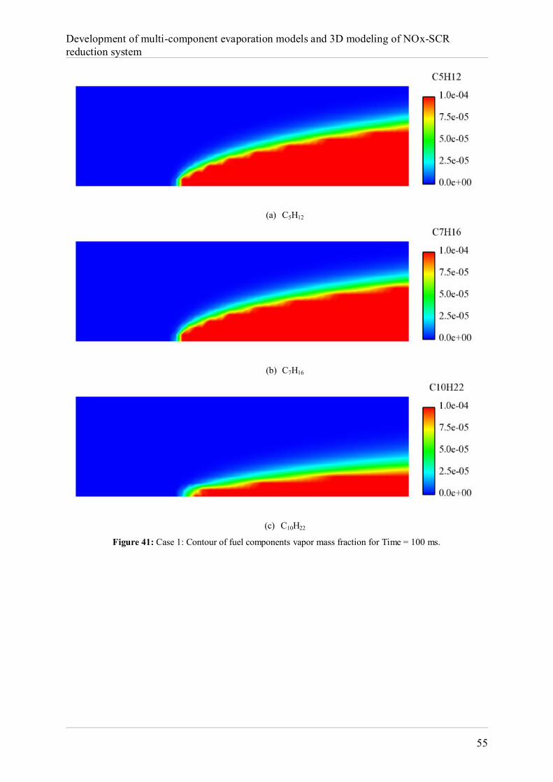
Development of multi-component evaporation models and 3D modeling of NOx-SCR reduction system
55
(a) C5H12
(b) C7H16
(c) C10H22
Figure 41: Case 1: Contour of fuel components vapor mass fraction for Time = 100 ms.
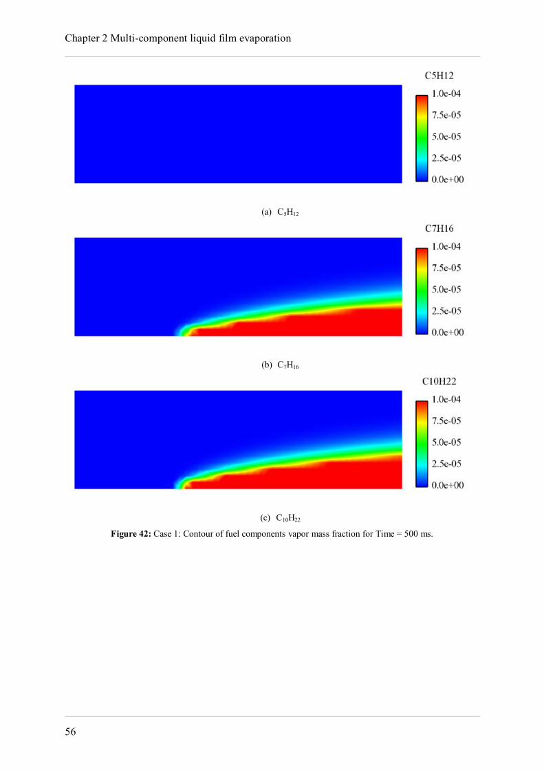
Chapter 2 Multi-component liquid film evaporation
56
(a) C5H12
(b) C7H16
(c) C10H22
Figure 42: Case 1: Contour of fuel components vapor mass fraction for Time = 500 ms.
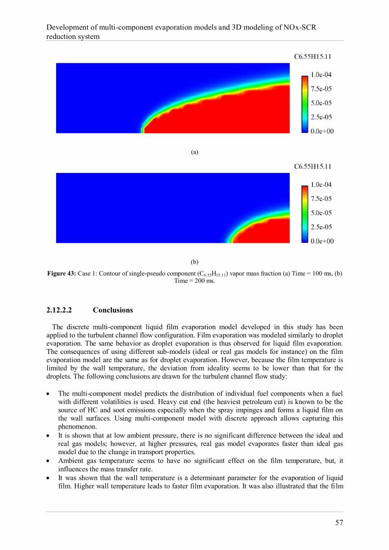
Development of multi-component evaporation models and 3D modeling of NOx-SCR reduction system
57
(a)
(b)
Figure 43: Case 1: Contour of single-pseudo component (C6.55H15.11) vapor mass fraction (a) Time = 100 ms, (b) Time = 200 ms.
2.12.2.2 Conclusions The discrete multi-component liquid film evaporation model developed in this study has been applied to the turbulent channel flow configuration. Film evaporation was modeled similarly to droplet evaporation. The same behavior as droplet evaporation is thus observed for liquid film evaporation. The consequences of using different sub-models (ideal or real gas models for instance) on the film evaporation model are the same as for droplet evaporation. However, because the film temperature is limited by the wall temperature, the deviation from ideality seems to be lower than that for the droplets. The following conclusions are drawn for the turbulent channel flow study: The multi-component model predicts the distribution of individual fuel components when a fuel
with different volatilities is used. Heavy cut end (the heaviest petroleum cut) is known to be the source of HC and soot emissions especially when the spray impinges and forms a liquid film on the wall surfaces. Using multi-component model with discrete approach allows capturing this phenomenon.
It is shown that at low ambient pressure, there is no significant difference between the ideal and real gas models; however, at higher pressures, real gas model evaporates faster than ideal gas model due to the change in transport properties.
Ambient gas temperature seems to have no significant effect on the film temperature, but, it influences the mass transfer rate.
It was shown that the wall temperature is a determinant parameter for the evaporation of liquid film. Higher wall temperature leads to faster film evaporation. It was also illustrated that the fi lm
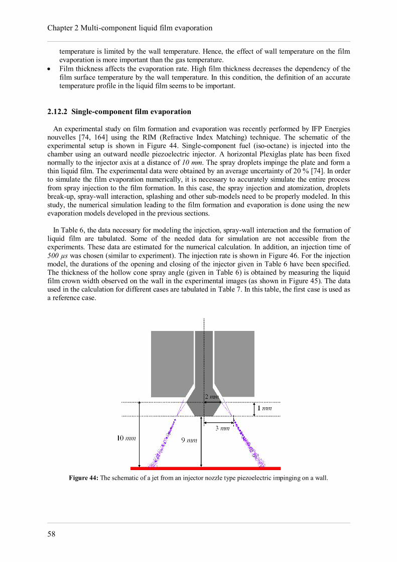
Chapter 2 Multi-component liquid film evaporation
58
temperature is limited by the wall temperature. Hence, the effect of wall temperature on the film evaporation is more important than the gas temperature.
Film thickness affects the evaporation rate. High film thickness decreases the dependency of the film surface temperature by the wall temperature. In this condition, the definition of an accurate temperature profile in the liquid film seems to be important.
2.12.2 Single-component film evaporation An experimental study on film formation and evaporation was recently performed by IFP Energies nouvelles [74, 164] using the RIM (Refractive Index Matching) technique. The schematic of the experimental setup is shown in Figure 44. Single-component fuel (iso-octane) is injected into the chamber using an outward needle piezoelectric injector. A horizontal Plexiglas plate has been fixed normally to the injector axis at a distance of 10 mm. The spray droplets impinge the plate and form a thin liquid film. The experimental data were obtained by an average uncertainty of 20 % [74]. In order to simulate the film evaporation numerically, it is necessary to accurately simulate the entire process from spray injection to the film formation. In this case, the spray injection and atomization, droplets break-up, spray-wall interaction, splashing and other sub-models need to be properly modeled. In this study, the numerical simulation leading to the film formation and evaporation is done using the new evaporation models developed in the previous sections. In Table 6, the data necessary for modeling the injection, spray-wall interaction and the formation of liquid film are tabulated. Some of the needed data for simulation are not accessible from the experiments. These data are estimated for the numerical calculation. In addition, an injection time of 500 µs was chosen (similar to experiment). The injection rate is shown in Figure 46. For the injection model, the durations of the opening and closing of the injector given in Table 6 have been specified. The thickness of the hollow cone spray angle (given in Table 6) is obtained by measuring the liquid film crown width observed on the wall in the experimental images (as shown in Figure 45). The data used in the calculation for different cases are tabulated in Table 7. In this table, the first case is used as a reference case.
Figure 44: The schematic of a jet from an injector nozzle type piezoelectric impinging on a wall.
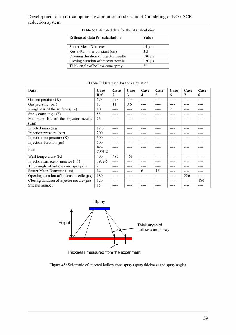
Development of multi-component evaporation models and 3D modeling of NOx-SCR reduction system
59
Table 6: Estimated data for the 3D calculation
Estimated data for calculation
Value
Sauter Mean Diameter 14 µm Rosin-Rammler constant (crr) 3.5 Opening duration of injector needle 180 µs Closing duration of injector needle 120 µs Thick angle of hollow cone spray 2°
Table 7: Data used for the calculation
Data Case Ref.
Case 2
Case 3
Case 4
Case 5
Case 6
Case 7
Case 8
Gas temperature (K) 673 573 453 ---- ---- ---- ---- ---- Gas pressure (bar) 13 11 8.6 ---- ---- ---- ---- ---- Roughness of the surface (µm) 10 ---- ---- ---- ---- 2 ---- ---- Spray cone angle (°) 85 ---- ---- ---- ---- ---- ---- ---- Maximum lift of the injector needle (µm)
26 ---- ---- ---- ---- ---- ---- ----
Injected mass (mg) 12.3 ---- ---- ---- ---- ---- ---- ---- Injection pressure (bar) 200 ---- ---- ---- ---- ---- ---- ---- Injection temperature (K) 300 ---- ---- ---- ---- ---- ---- ---- Injection duration (µs) 500 ---- ---- ---- ---- ---- ---- ----
Fuel Iso-C8H18
---- ---- ---- ---- ---- ---- ----
Wall temperature (K) 490 487 468 ---- ---- ---- ---- ---- Injection surface of injector (m2) 397e-6 ---- ---- ---- ---- ---- ---- ---- Thick angle of hollow cone spray (°) 2 ---- ---- ---- ---- ---- ---- ---- Sauter Mean Diameter (µm) 14 ---- ---- 6 18 ---- ---- ---- Opening duration of injector needle (µs) 180 ---- ---- ---- ---- ---- 220 ---- Closing duration of injector needle (µs) 120 ---- ---- ---- ---- ---- ---- 180 Streaks number 15 ---- ---- ---- ---- ---- ---- ----
Figure 45: Schematic of injected hollow cone spray (spray thickness and spray angle).
Thickness measured from the experiment
Thick angle of hollow-cone spray
Height
Spray
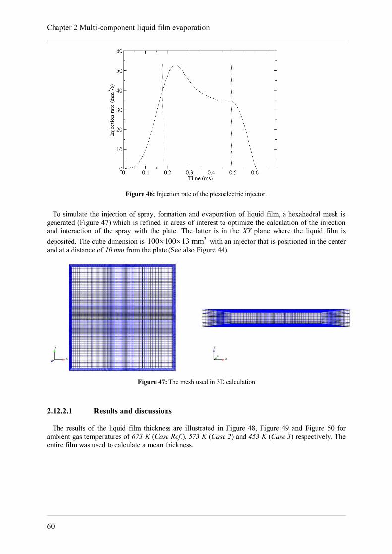
Chapter 2 Multi-component liquid film evaporation
60
Figure 46: Injection rate of the piezoelectric injector.
To simulate the injection of spray, formation and evaporation of liquid film, a hexahedral mesh is generated (Figure 47) which is refined in areas of interest to optimize the calculation of the injection and interaction of the spray with the plate. The latter is in the XY plane where the liquid film is deposited. The cube dimension is 3100 100 13 mm with an injector that is positioned in the center and at a distance of 10 mm from the plate (See also Figure 44).
Figure 47: The mesh used in 3D calculation
2.12.2.1 Results and discussions The results of the liquid film thickness are illustrated in Figure 48, Figure 49 and Figure 50 for ambient gas temperatures of 673 K (Case Ref.), 573 K (Case 2) and 453 K (Case 3) respectively. The entire film was used to calculate a mean thickness.
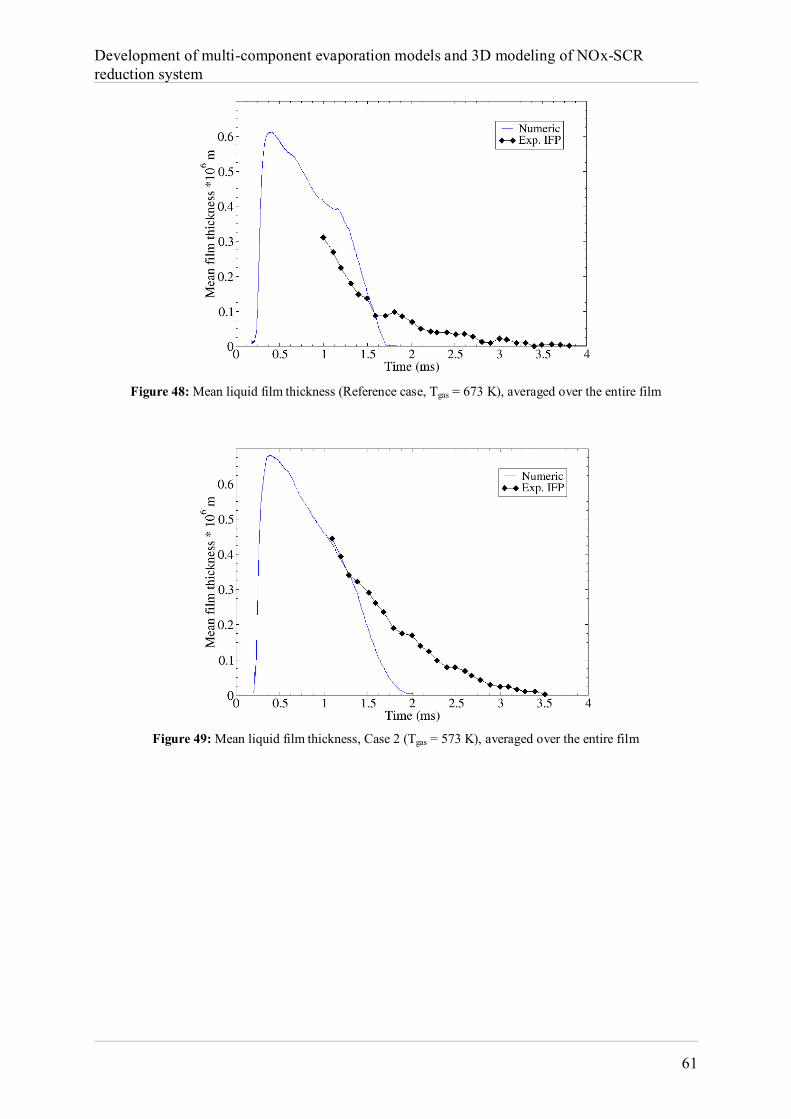
Development of multi-component evaporation models and 3D modeling of NOx-SCR reduction system
61
Figure 48: Mean liquid film thickness (Reference case, Tgas = 673 K), averaged over the entire film
Figure 49: Mean liquid film thickness, Case 2 (Tgas = 573 K), averaged over the entire film
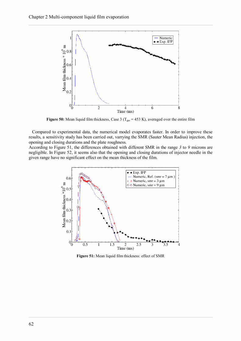
Chapter 2 Multi-component liquid film evaporation
62
Figure 50: Mean liquid film thickness, Case 3 (Tgas = 453 K), averaged over the entire film
Compared to experimental data, the numerical model evaporates faster. In order to improve these results, a sensitivity study has been carried out, varrying the SMR (Sauter Mean Radius) injection, the opening and closing durations and the plate roughness. According to Figure 51, the differences obtained with different SMR in the range 3 to 9 microns are negligible. In Figure 52, it seems also that the opening and closing durations of injector needle in the given range have no significant effect on the mean thickness of the film.
Figure 51: Mean liquid film thickness: effect of SMR
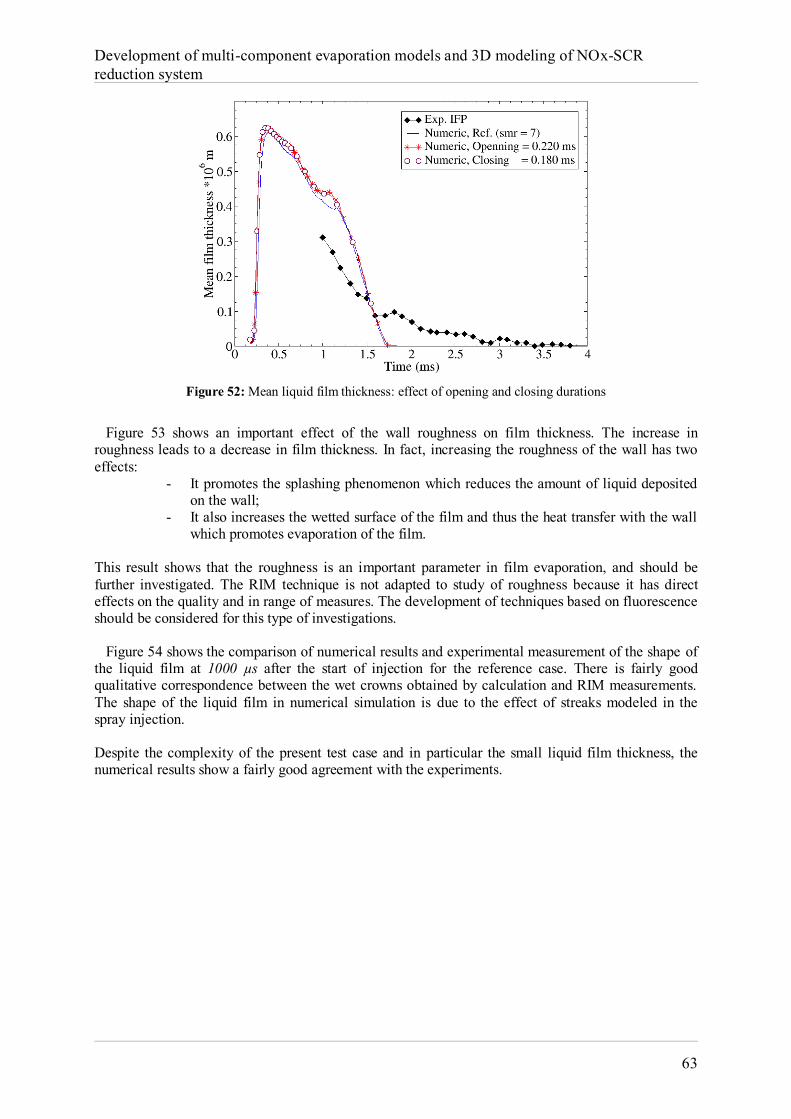
Development of multi-component evaporation models and 3D modeling of NOx-SCR reduction system
63
Figure 52: Mean liquid film thickness: effect of opening and closing durations
Figure 53 shows an important effect of the wall roughness on film thickness. The increase in roughness leads to a decrease in film thickness. In fact, increasing the roughness of the wall has two effects:
- It promotes the splashing phenomenon which reduces the amount of liquid deposited on the wall;
- It also increases the wetted surface of the film and thus the heat transfer with the wall which promotes evaporation of the film.
This result shows that the roughness is an important parameter in film evaporation, and should be further investigated. The RIM technique is not adapted to study of roughness because it has direct effects on the quality and in range of measures. The development of techniques based on fluorescence should be considered for this type of investigations. Figure 54 shows the comparison of numerical results and experimental measurement of the shape of the liquid film at 1000 µs after the start of injection for the reference case. There is fairly good qualitative correspondence between the wet crowns obtained by calculation and RIM measurements. The shape of the liquid film in numerical simulation is due to the effect of streaks modeled in the spray injection. Despite the complexity of the present test case and in particular the small liquid film thickness, the numerical results show a fairly good agreement with the experiments.
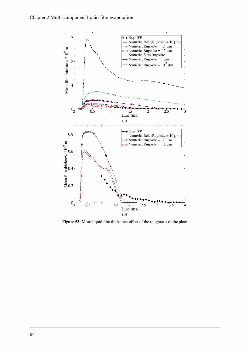
Chapter 2 Multi-component liquid film evaporation
64
(a)
(b)
Figure 53: Mean liquid film thickness: effect of the roughness of the plate
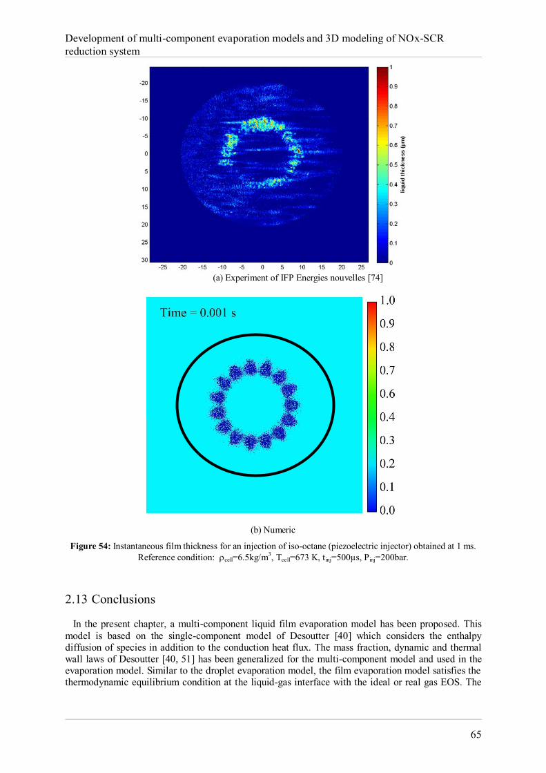
Development of multi-component evaporation models and 3D modeling of NOx-SCR reduction system
65
(a) Experiment of IFP Energies nouvelles [74]
(b) Numeric
Figure 54: Instantaneous film thickness for an injection of iso-octane (piezoelectric injector) obtained at 1 ms. Reference condition: cell=6.5kg/m3, Tcell=673 K, tinj=500µs, Pinj=200bar.
2.13 Conclusions In the present chapter, a multi-component liquid film evaporation model has been proposed. This model is based on the single-component model of Desoutter [40] which considers the enthalpy diffusion of species in addition to the conduction heat flux. The mass fraction, dynamic and thermal wall laws of Desoutter [40, 51] has been generalized for the multi-component model and used in the evaporation model. Similar to the droplet evaporation model, the film evaporation model satisfies the thermodynamic equilibrium condition at the liquid-gas interface with the ideal or real gas EOS. The
Chapter 2 Multi-component liquid film evaporation
66
liquid film model developed in the present study has been applied to the turbulent channel flow and wall-spray test cases. The main conclusions of the present study are as follows: The availability of the multi-component liquid film evaporation model is a step forward towards
predicting the detailed behaviors of species in internal combustion engines. As a single-pseudo component fuel model may not represent the behavior of an actual fuel, the
availability of a multi-component evaporation model makes it possible to use more representative fuel models in future simulations.
The availability of the database RIM is a good opportunity to improve and validate 3D models of liquid film in CFD code. It would be desirable to supplement the base RIM by the cases where the liquid film is thicker. Indeed, thicker liquid films may be present in the operating conditions such as cold starts, for example. On the other hand, it would be interesting to confirm by further experiments the strong sensitivity of the models to the roughness value. For this, the use of plates of smaller roughness (0.1 to 1 µm) is desirable.
Comparison of the film model with some experimental data for multi-component fuels is still necessary.
In the next chapter, the effects of multi-component droplet and film evaporation models on the mixture preparation and combustion in internal engine test cases will be investigated using IFP-C3D code.
Chapter 3
Application of the proposed evaporation
models in Diesel engine 3.1 Multi-component diesel engine computation The aim of the present chapter is to highlight the benefits of using the multi-component evaporation models for the computation of Diesel engines. A numerical study of the mixture preparation and combustion of a multi-component diesel fuel has been performed in the NADI concept (Narrow Angle Direct Injection) of diesel engine using IFP-C3D code [139]. General structure of IFP-C3D code is described in Appendix E. Main physical models included in IFP-C3D for liquid spray modeling are the new multi-component evaporation model proposed in the present study, the Wave-FIPA breakup model [166], the spray-wall interaction models including liquid film transport, evaporation (developed in this work) and boiling [152]. For combustion modeling, IFP-C3D includes the auto-ignition TKI model [167], the spark plug ignition AKTIM model [168] and the ECFM3Z Diesel combustion model [169]. These models enable the simulation of a large variety of innovative fuel and engine configurations and have been used in the present work. The gas ideality hypothesis and single/multi-component fuel evaporation models are investigated. Note that the real gas model is used only for the liquid-gas equilibrium at the liquid-gas interface while using the ideal gas hypothesis for the gas at the infinity. 3.1.1 Detail of the methodology of the calculation In order to simulate the engine mixture preparation and combustion using IFP-C3D code, the diesel fuel is lumped in a single Dfl1 or three (Dfl3a, Dfl3b and Dfl3c) pseudo-components by the initial composition of real components [149, 170, 171]. Until now, the unavailability of a multi-component film model in IFP-C3D code limited CFD calculations to single-component fuel. The new multi-component evaporation models allow for the first time to study different compositions of real or pseudo-component. In this chapter, the numerical results of the engine test case with single-component diesel fuel and its three-pseudo representation will be compared using ideal and real gas models. The numerical results will not be compared to experimental data as real engine parameters and conditions could not be simulated. The engine parameters and injection specifications used for the simulation of a typical Diesel engine are presented in Table 8. The schematic of one-sixth sector of the cylinder of the engine
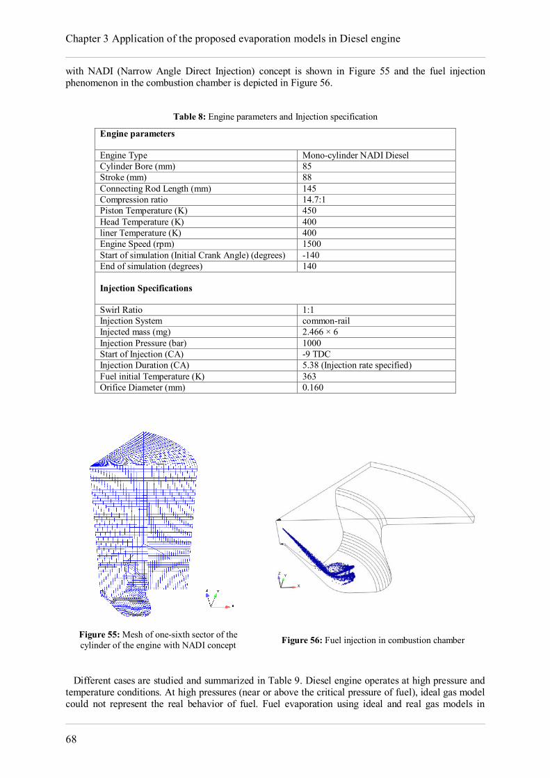
Chapter 3 Application of the proposed evaporation models in Diesel engine
68
with NADI (Narrow Angle Direct Injection) concept is shown in Figure 55 and the fuel injection phenomenon in the combustion chamber is depicted in Figure 56.
Table 8: Engine parameters and Injection specification
Engine parameters Engine Type Mono-cylinder NADI Diesel Cylinder Bore (mm) 85 Stroke (mm) 88 Connecting Rod Length (mm) 145 Compression ratio 14.7:1 Piston Temperature (K) 450 Head Temperature (K) 400 liner Temperature (K) 400 Engine Speed (rpm) 1500 Start of simulation (Initial Crank Angle) (degrees) -140 End of simulation (degrees) 140 Injection Specifications Swirl Ratio 1:1 Injection System common-rail Injected mass (mg) 2.466 × 6 Injection Pressure (bar) 1000 Start of Injection (CA) -9 TDC Injection Duration (CA) 5.38 (Injection rate specified) Fuel initial Temperature (K) 363 Orifice Diameter (mm) 0.160
Figure 55: Mesh of one-sixth sector of the cylinder of the engine with NADI concept Figure 56: Fuel injection in combustion chamber
Different cases are studied and summarized in Table 9. Diesel engine operates at high pressure and temperature conditions. At high pressures (near or above the critical pressure of fuel), ideal gas model could not represent the real behavior of fuel. Fuel evaporation using ideal and real gas models in
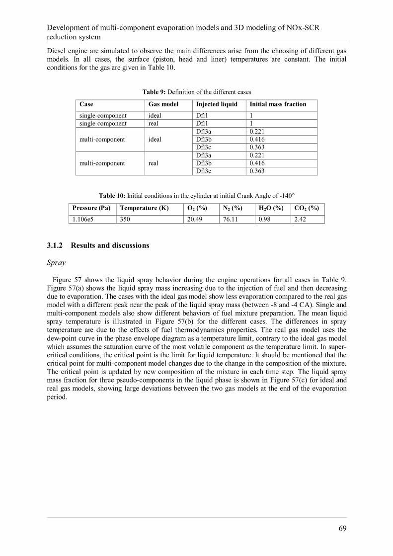
Development of multi-component evaporation models and 3D modeling of NOx-SCR reduction system
69
Diesel engine are simulated to observe the main differences arise from the choosing of different gas models. In all cases, the surface (piston, head and liner) temperatures are constant. The initial conditions for the gas are given in Table 10.
Table 9: Definition of the different cases
Case Gas model Injected liquid Initial mass fraction
single-component ideal Dfl1 1 single-component real Dfl1 1
multi-component ideal Dfl3a 0.221 Dfl3b 0.416 Dfl3c 0.363
multi-component real Dfl3a 0.221 Dfl3b 0.416 Dfl3c 0.363
Table 10: Initial conditions in the cylinder at initial Crank Angle of -140°
Pressure (Pa) Temperature (K) O2 (%) N2 (%) H2O (%) CO2 (%)
1.106e5 350 20.49 76.11 0.98 2.42 3.1.2 Results and discussions Spray Figure 57 shows the liquid spray behavior during the engine operations for all cases in Table 9. Figure 57(a) shows the liquid spray mass increasing due to the injection of fuel and then decreasing due to evaporation. The cases with the ideal gas model show less evaporation compared to the real gas model with a different peak near the peak of the liquid spray mass (between -8 and -4 CA). Single and multi-component models also show different behaviors of fuel mixture preparation. The mean liquid spray temperature is illustrated in Figure 57(b) for the different cases. The differences in spray temperature are due to the effects of fuel thermodynamics properties. The real gas model uses the dew-point curve in the phase envelope diagram as a temperature limit, contrary to the ideal gas model which assumes the saturation curve of the most volatile component as the temperature limit. In super-critical conditions, the critical point is the limit for liquid temperature. It should be mentioned that the critical point for multi-component model changes due to the change in the composition of the mixture. The critical point is updated by new composition of the mixture in each time step. The liquid spray mass fraction for three pseudo-components in the liquid phase is shown in Figure 57(c) for ideal and real gas models, showing large deviations between the two gas models at the end of the evaporation period.
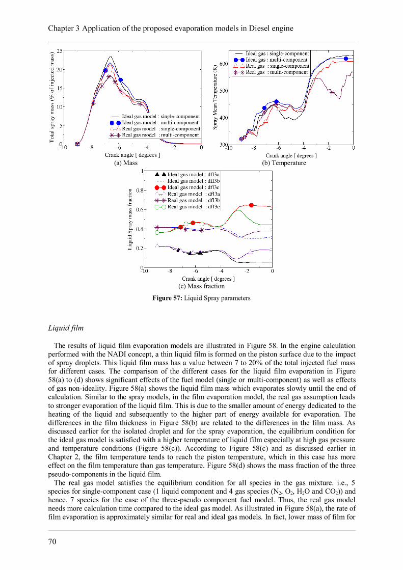
Chapter 3 Application of the proposed evaporation models in Diesel engine
70
(a) Mass (b) Temperature
(c) Mass fraction
Figure 57: Liquid Spray parameters
Liquid film The results of liquid film evaporation models are illustrated in Figure 58. In the engine calculation performed with the NADI concept, a thin liquid film is formed on the piston surface due to the impact of spray droplets. This liquid film mass has a value between 7 to 20% of the total injected fuel mass for different cases. The comparison of the different cases for the liquid film evaporation in Figure 58(a) to (d) shows significant effects of the fuel model (single or multi-component) as well as effects of gas non-ideality. Figure 58(a) shows the liquid film mass which evaporates slowly until the end of calculation. Similar to the spray models, in the film evaporation model, the real gas assumption leads to stronger evaporation of the liquid film. This is due to the smaller amount of energy dedicated to the heating of the liquid and subsequently to the higher part of energy available for evaporation. The differences in the film thickness in Figure 58(b) are related to the differences in the film mass. As discussed earlier for the isolated droplet and for the spray evaporation, the equilibrium condition for the ideal gas model is satisfied with a higher temperature of liquid film especially at high gas pressure and temperature conditions (Figure 58(c)). According to Figure 58(c) and as discussed earlier in Chapter 2, the film temperature tends to reach the piston temperature, which in this case has more effect on the film temperature than gas temperature. Figure 58(d) shows the mass fraction of the three pseudo-components in the liquid film. The real gas model satisfies the equilibrium condition for all species in the gas mixture. i.e., 5 species for single-component case (1 liquid component and 4 gas species (N2, O2, H2O and CO2)) and hence, 7 species for the case of the three-pseudo component fuel model. Thus, the real gas model needs more calculation time compared to the ideal gas model. As illustrated in Figure 58(a), the rate of film evaporation is approximately similar for real and ideal gas models. In fact, lower mass of film for
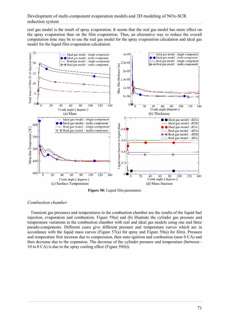
Development of multi-component evaporation models and 3D modeling of NOx-SCR reduction system
71
real gas model is the result of spray evaporation. It seems that the real gas model has more effect on the spray evaporation than on the film evaporation. Thus, an alternative way to reduce the overall computation time may be to use the real gas model for the spray evaporation calculation and ideal gas model for the liquid film evaporation calculation.
(a) Mass (b) Thickness
(c) Surface Temperature (d) Mass fraction
Figure 58: Liquid film parameters
Combustion chamber Transient gas pressures and temperatures in the combustion chamber are the results of the liquid fuel injection, evaporation and combustion. Figure 59(a) and (b) illustrate the cylinder gas pressure and temperature variations in the combustion chamber with real and ideal gas models using one and three pseudo-components. Different cases give different pressure and temperature curves which are in accordance with the liquid mass curves (Figure 57(a) for spray and Figure 58(a) for film). Pressure and temperature first increase due to compression, then auto-ignition and combustion (near 0 CA) and then decrease due to the expansion. The decrease of the cylinder pressure and temperature (between -10 to 0 CA) is due to the spray cooling effect (Figure 59(b)).
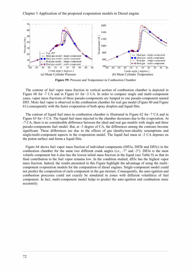
Chapter 3 Application of the proposed evaporation models in Diesel engine
72
(a) Mean Cylinder Pressure (b) Mean Cylinder Temperature
Figure 59: Pressure and Temperature in Combustion Chamber
The contour of fuel vapor mass fraction in vertical section of combustion chamber is depicted in Figure 60 for -7 CA and in Figure 61 for -3 CA. In order to compare single and multi-component cases, vapor mass fractions of three pseudo-components are lumped to one pseudo-component named Dfl3. More fuel vapor is observed in the combustion chamber for real gas model (Figure 60 and Figure 61) consequently with the faster evaporation of both spray droplets and liquid film. The contour of liquid fuel mass in combustion chamber is illustrated in Figure 62 for -7 CA and in Figure 63 for -3 CA. The liquid fuel mass injected to the chamber decreases due to the evaporation. At -7 CA, there is no considerable difference between the ideal and real gas models with single and three pseudo-components fuel model. But, at -3 degree of CA, the differences among the contours become significant. These differences are due to the effects of gas ideality/non-ideality assumptions and single/multi-component aspects in the evaporation model. The liquid fuel mass at -3 CA deposes on the piston surface and forms a liquid film. Figure 64 shows fuel vapor mass fraction of individual components (Dfl3a, Dfl3b and Dfl3c) in the combustion chamber for the same two different crank angles (i.e., -7° and -3°). Dfl3a is the most volatile component but it also has the lowest initial mass fraction in the liquid (see Table 9) so that its final contribution to the fuel vapor remains low. In the condition studied, dfl3c has the highest vapor mass fraction. Indeed, the results presented in this Figure highlight the advantage of using the multi-component evaporation models for the computation of diesel engines. Single-component model could not predict the composition of each component in the gas mixture. Consequently, the auto-ignition and combustion processes could not exactly be simulated in zones with different volatilities of fuel component. In fact, multi-component model helps to predict the auto-ignition and combustion more accurately.
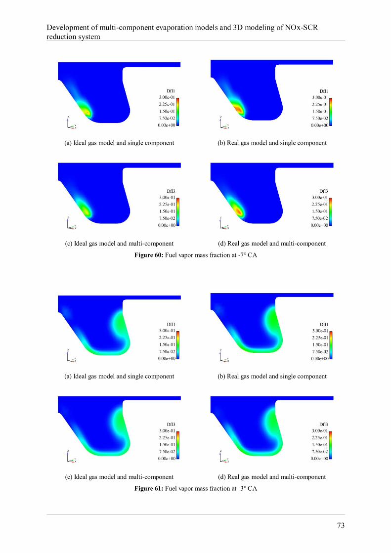
Development of multi-component evaporation models and 3D modeling of NOx-SCR reduction system
73
(a) Ideal gas model and single component (b) Real gas model and single component
(c) Ideal gas model and multi-component (d) Real gas model and multi-component
Figure 60: Fuel vapor mass fraction at -7° CA
(a) Ideal gas model and single component (b) Real gas model and single component
(c) Ideal gas model and multi-component (d) Real gas model and multi-component
Figure 61: Fuel vapor mass fraction at -3° CA
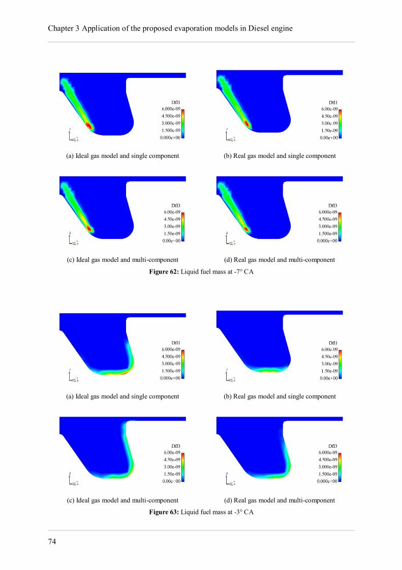
Chapter 3 Application of the proposed evaporation models in Diesel engine
74
(a) Ideal gas model and single component (b) Real gas model and single component
(c) Ideal gas model and multi-component (d) Real gas model and multi-component
Figure 62: Liquid fuel mass at -7° CA
(a) Ideal gas model and single component (b) Real gas model and single component
(c) Ideal gas model and multi-component (d) Real gas model and multi-component
Figure 63: Liquid fuel mass at -3° CA
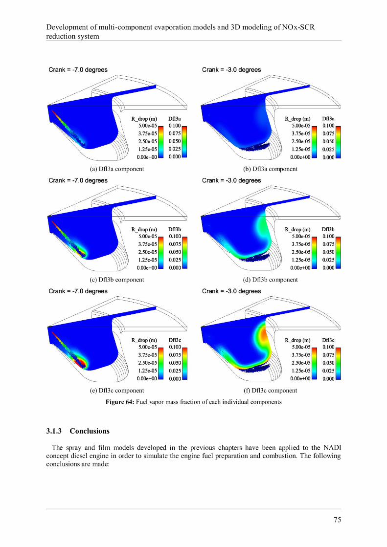
Development of multi-component evaporation models and 3D modeling of NOx-SCR reduction system
75
(a) Dfl3a component (b) Dfl3a component
(c) Dfl3b component (d) Dfl3b component
(e) Dfl3c component (f) Dfl3c component
Figure 64: Fuel vapor mass fraction of each individual components
3.1.3 Conclusions The spray and film models developed in the previous chapters have been applied to the NADI concept diesel engine in order to simulate the engine fuel preparation and combustion. The following conclusions are made:
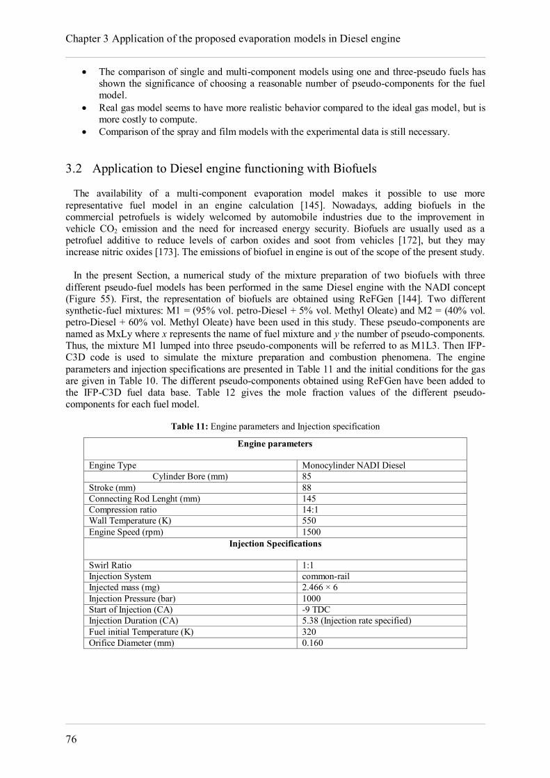
Chapter 3 Application of the proposed evaporation models in Diesel engine
76
The comparison of single and multi-component models using one and three-pseudo fuels has shown the significance of choosing a reasonable number of pseudo-components for the fuel model.
Real gas model seems to have more realistic behavior compared to the ideal gas model, but is more costly to compute.
Comparison of the spray and film models with the experimental data is still necessary. 3.2 Application to Diesel engine functioning with Biofuels The availability of a multi-component evaporation model makes it possible to use more representative fuel model in an engine calculation [145]. Nowadays, adding biofuels in the commercial petrofuels is widely welcomed by automobile industries due to the improvement in vehicle CO2 emission and the need for increased energy security. Biofuels are usually used as a petrofuel additive to reduce levels of carbon oxides and soot from vehicles [172], but they may increase nitric oxides [173]. The emissions of biofuel in engine is out of the scope of the present study. In the present Section, a numerical study of the mixture preparation of two biofuels with three different pseudo-fuel models has been performed in the same Diesel engine with the NADI concept (Figure 55). First, the representation of biofuels are obtained using ReFGen [144]. Two different synthetic-fuel mixtures: M1 = (95% vol. petro-Diesel + 5% vol. Methyl Oleate) and M2 = (40% vol. petro-Diesel + 60% vol. Methyl Oleate) have been used in this study. These pseudo-components are named as MxLy where x represents the name of fuel mixture and y the number of pseudo-components. Thus, the mixture M1 lumped into three pseudo-components will be referred to as M1L3. Then IFP-C3D code is used to simulate the mixture preparation and combustion phenomena. The engine parameters and injection specifications are presented in Table 11 and the initial conditions for the gas are given in Table 10. The different pseudo-components obtained using ReFGen have been added to the IFP-C3D fuel data base. Table 12 gives the mole fraction values of the different pseudo-components for each fuel model.
Table 11: Engine parameters and Injection specification
Engine parameters
Engine Type Monocylinder NADI Diesel Cylinder Bore (mm) 85
Stroke (mm) 88 Connecting Rod Lenght (mm) 145 Compression ratio 14:1 Wall Temperature (K) 550 Engine Speed (rpm) 1500
Injection Specifications
Swirl Ratio 1:1 Injection System common-rail Injected mass (mg) 2.466 × 6 Injection Pressure (bar) 1000 Start of Injection (CA) -9 TDC Injection Duration (CA) 5.38 (Injection rate specified) Fuel initial Temperature (K) 320 Orifice Diameter (mm) 0.160
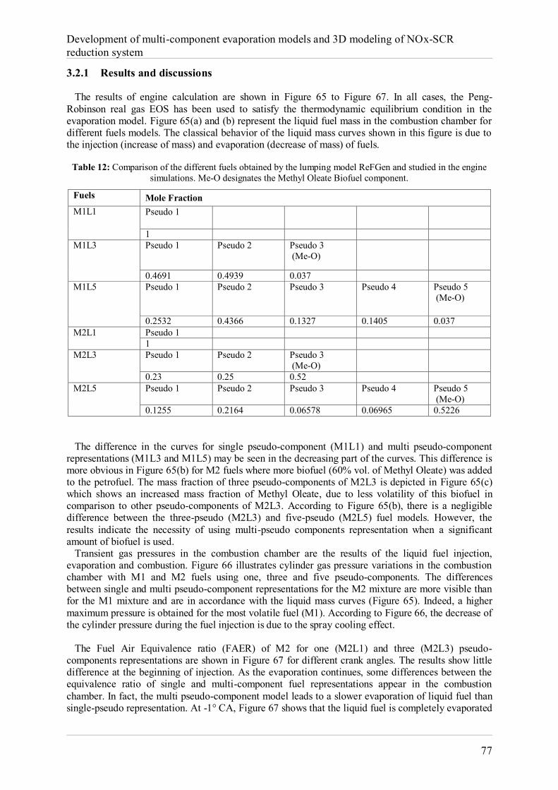
Development of multi-component evaporation models and 3D modeling of NOx-SCR reduction system
77
3.2.1 Results and discussions The results of engine calculation are shown in Figure 65 to Figure 67. In all cases, the Peng-Robinson real gas EOS has been used to satisfy the thermodynamic equilibrium condition in the evaporation model. Figure 65(a) and (b) represent the liquid fuel mass in the combustion chamber for different fuels models. The classical behavior of the liquid mass curves shown in this figure is due to the injection (increase of mass) and evaporation (decrease of mass) of fuels.
Table 12: Comparison of the different fuels obtained by the lumping model ReFGen and studied in the engine simulations. Me-O designates the Methyl Oleate Biofuel component.
Fuels Mole Fraction M1L1 Pseudo 1
1 M1L3 Pseudo 1 Pseudo 2 Pseudo 3
(Me-O)
0.4691 0.4939 0.037 M1L5 Pseudo 1 Pseudo 2 Pseudo 3 Pseudo 4 Pseudo 5
(Me-O)
0.2532 0.4366 0.1327 0.1405 0.037 M2L1 Pseudo 1
1 M2L3 Pseudo 1 Pseudo 2 Pseudo 3
(Me-O)
0.23 0.25 0.52 M2L5 Pseudo 1 Pseudo 2 Pseudo 3 Pseudo 4 Pseudo 5
(Me-O) 0.1255 0.2164 0.06578 0.06965 0.5226
The difference in the curves for single pseudo-component (M1L1) and multi pseudo-component representations (M1L3 and M1L5) may be seen in the decreasing part of the curves. This difference is more obvious in Figure 65(b) for M2 fuels where more biofuel (60% vol. of Methyl Oleate) was added to the petrofuel. The mass fraction of three pseudo-components of M2L3 is depicted in Figure 65(c) which shows an increased mass fraction of Methyl Oleate, due to less volatility of this biofuel in comparison to other pseudo-components of M2L3. According to Figure 65(b), there is a negligible difference between the three-pseudo (M2L3) and five-pseudo (M2L5) fuel models. However, the results indicate the necessity of using multi-pseudo components representation when a significant amount of biofuel is used. Transient gas pressures in the combustion chamber are the results of the liquid fuel injection, evaporation and combustion. Figure 66 illustrates cylinder gas pressure variations in the combustion chamber with M1 and M2 fuels using one, three and five pseudo-components. The differences between single and multi pseudo-component representations for the M2 mixture are more visible than for the M1 mixture and are in accordance with the liquid mass curves (Figure 65). Indeed, a higher maximum pressure is obtained for the most volatile fuel (M1). According to Figure 66, the decrease of the cylinder pressure during the fuel injection is due to the spray cooling effect. The Fuel Air Equivalence ratio (FAER) of M2 for one (M2L1) and three (M2L3) pseudo-components representations are shown in Figure 67 for different crank angles. The results show little difference at the beginning of injection. As the evaporation continues, some differences between the equivalence ratio of single and multi-component fuel representations appear in the combustion chamber. In fact, the multi pseudo-component model leads to a slower evaporation of liquid fuel than single-pseudo representation. At -1° CA, Figure 67 shows that the liquid fuel is completely evaporated
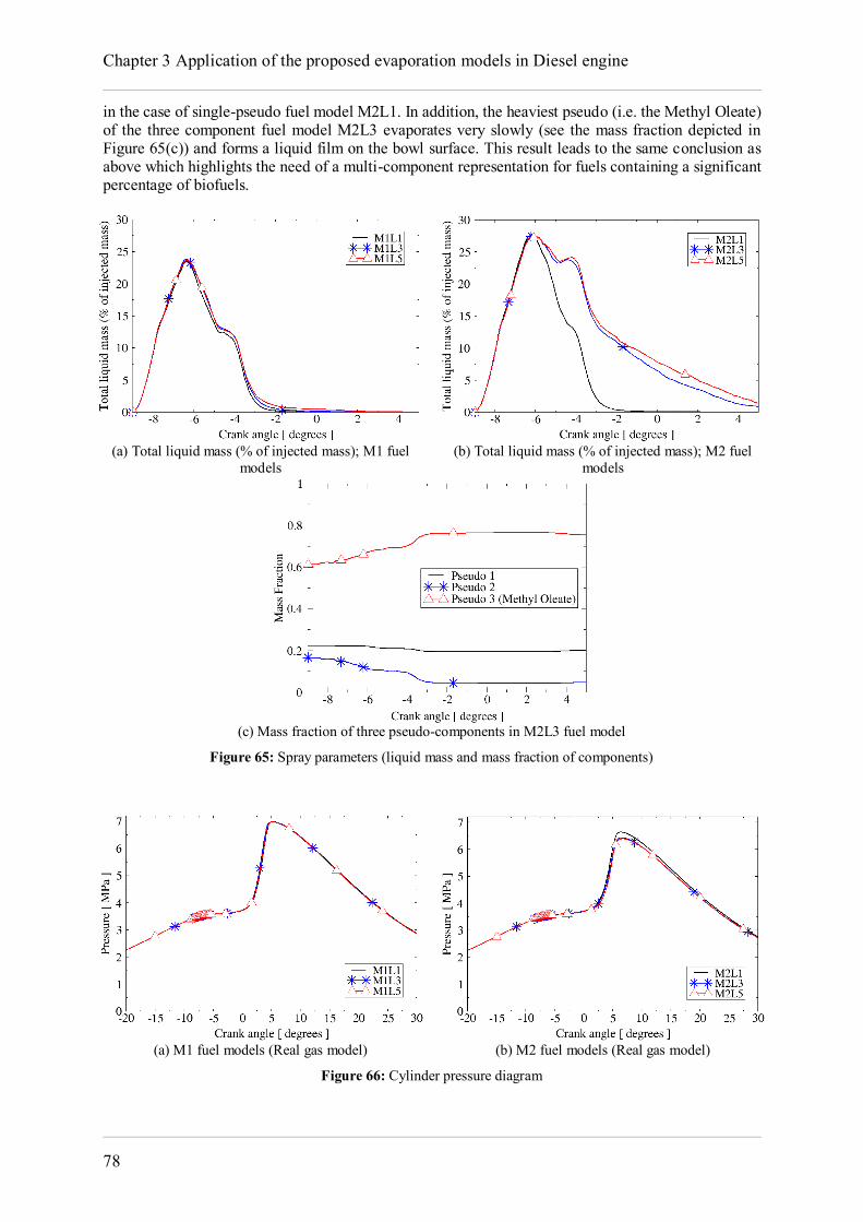
Chapter 3 Application of the proposed evaporation models in Diesel engine
78
in the case of single-pseudo fuel model M2L1. In addition, the heaviest pseudo (i.e. the Methyl Oleate) of the three component fuel model M2L3 evaporates very slowly (see the mass fraction depicted in Figure 65(c)) and forms a liquid film on the bowl surface. This result leads to the same conclusion as above which highlights the need of a multi-component representation for fuels containing a significant percentage of biofuels.
(a) Total liquid mass (% of injected mass); M1 fuel
models (b) Total liquid mass (% of injected mass); M2 fuel
models
(c) Mass fraction of three pseudo-components in M2L3 fuel model
Figure 65: Spray parameters (liquid mass and mass fraction of components)
(a) M1 fuel models (Real gas model) (b) M2 fuel models (Real gas model)
Figure 66: Cylinder pressure diagram
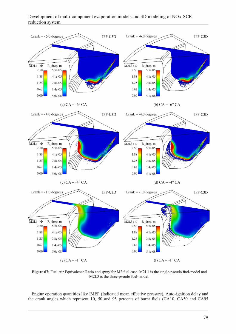
Development of multi-component evaporation models and 3D modeling of NOx-SCR reduction system
79
(a) CA = -6° CA
(b) CA = -6° CA
(c) CA = -4° CA
(d) CA = -4° CA
(e) CA = -1° CA
(f) CA = -1° CA
Figure 67: Fuel Air Equivalence Ratio and spray for M2 fuel case. M2L1 is the single-pseudo fuel-model and M2L3 is the three-pseudo fuel-model.
Engine operation quantities like IMEP (Indicated mean effective pressure), Auto-ignition delay and the crank angles which represent 10, 50 and 95 percents of burnt fuels (CA10, CA50 and CA95
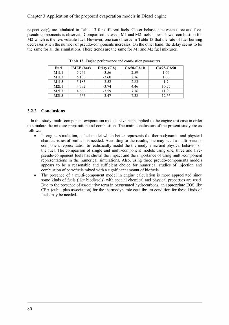
Chapter 3 Application of the proposed evaporation models in Diesel engine
80
respectively), are tabulated in Table 13 for different fuels. Closer behavior between three and five-pseudo components is observed. Comparison between M1 and M2 fuels shows slower combustion for M2 which is the less volatile fuel. However, one can observe in Table 13 that the rate of fuel burning decreases when the number of pseudo-components increases. On the other hand, the delay seems to be the same for all the simulations. These trends are the same for M1 and M2 fuel mixtures.
Table 13: Engine performance and combustion parameters
Fuel IMEP (bar) Delay (CA) CA50-CA10 CA95-CA50 M1L1 5.245 -3.56 2.59 1.66 M1L3 5.186 -3.60 2.76 1.66 M1L5 5.185 -3.52 2.83 1.7 M2L1 4.792 -3.74 4.46 10.75 M2L3 4.666 -3.59 7.16 11.96 M2L5 4.665 -3.47 7.38 12.66
3.2.2 Conclusions In this study, multi-component evaporation models have been applied to the engine test case in order to simulate the mixture preparation and combustion. The main conclusions of the present study are as follows:
In engine simulation, a fuel model which better represents the thermodynamic and physical characteristics of biofuels is needed. According to the results, one may need a multi pseudo-component representation to realistically model the thermodynamic and physical behavior of the fuel. The comparison of single and multi-component models using one, three and five-pseudo-component fuels has shown the impact and the importance of using multi-component representations in the numerical simulations. Also, using three pseudo-components models appears to be a reasonable and sufficient choice for numerical studies of injection and combustion of petrofuels mixed with a significant amount of biofuels.
The presence of a multi-component model in engine calculation is more appreciated since some kinds of fuels (like biodiesels) with special chemical and physical properties are used. Due to the presence of associative term in oxygenated hydrocarbons, an appropriate EOS like CPA (cubic plus association) for the thermodynamic equilibrium condition for these kinds of fuels may be needed.
Development of multi-component evaporation models and 3D modeling of NOx-SCR reduction system
81
Conclusions of Part I Lagrangian droplet and liquid film evaporation models using discrete multi-component approach have been suggested in the first part of this thesis manuscript. The evaporation models are based on the mass, momentum and energy conservation equations with no limitation in terms of the number of components in the liquid and gas phases. The multi-component droplet evaporation model is based on a Stephan velocity which recovers the mass conservation equation thanks to the Hirschfelder's law used for the diffusion velocity. The liquid film evaporation model is dedicated to turbulent flow conditions. Liquid film model equations are based on multi-component wall-laws generalized in the present work. Development of the mass, dynamic and thermal wall laws consist of resolving analytically the boundary layer equations on the surface of the wall or liquid film. In both droplet and liquid film models, the heat flux is assumed to be the summation of heat conduction and heat enthalpy diffusion of species. Indeed, the latter has been usually neglected in previous works. The evaporation models satisfy the thermodynamic equilibrium condition at the liquid-gas interface with the ideal or real gas EOS. The evaporation models were implemented into the multi-dimensional CFD RANS code (IFP-C3D). The evaporation models are first validated against the most recent experimental and numerical data and then used to simulate diesel engine mixture preparation with different fuel representations including biofuels. The following main conclusions were drawn during the present study: The numerical results of droplet evaporation model in comparison with the most recent
experimental data have shown that the heat flux due to the enthalpy diffusion of species could not be neglected in comparison to the conduction heat flux.
The calculated results characterize the vaporization processes of representative engine fuels and indicate the important influence of fuel volatility. The comparison with the results of single-component fuel also emphasizes the importance of considering multi-component effects in practical applications, especially for high-pressure and/or low temperature environments and for biofuels.
The comparison of single and multi-component models has shown the significance of choosing a reasonable number of pseudo-components for the fuel model. As a single-pseudo-component fuel-model may not represent the behavior of an actual fuel, the availability of a multi-component evaporation model makes it possible to use more representative fuel models in future simulations.
Almost similar total fuel mass evaporation of single and multi-component models for diesel engines at standard conditions may be due to the co-evaporation of most and less volatile components of diesel fuel. However, different behavior for single and multi-component biofuel is observed due to the different chemical structure of biofuels components.
High pressure aspects of fluids such as real gas EOS, mixture non-ideality and high pressure transport properties were addressed in the real gas model.
High pressure computations show a significant pressure influence on the evaporation rate. Different evaporation rates were obtained at high pressure conditions for real/ideal gas models. However, at low pressure conditions, the deviation from gas non-ideality becomes less important.
Real gas model seems to have more realistic behavior compared to the ideal gas model, but is more costly.
Finally, validation of the spray and film models with different experimental data is still necessary.
Chapter 3 Application of the proposed evaporation models in Diesel engine
82
Part II
SCR modeling
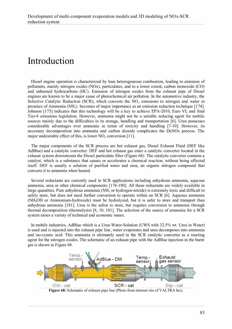
Development of multi-component evaporation models and 3D modeling of NOx-SCR reduction system
83
Introduction Diesel engine operation is characterized by lean heterogeneous combustion, leading to emission of pollutants, mainly nitrogen oxides (NOx), particulates, and to a lower extent, carbon monoxide (CO) and unburned hydrocarbons (HC). Emission of nitrogen oxides from the exhaust pipe of Diesel engines are known to be a major cause of photochemical air pollution. In the automotive industry, the Selective Catalytic Reduction (SCR), which converts the NOx emissions to nitrogen and water in presence of Ammonia (NH3) becomes of major importance as an emission reduction technique [174]. Johnson [175] indicates that this technology will be a key to achieve EPA-2010, Euro VI, and final Tier-4 emissions legislation. However, ammonia might not be a suitable reducing agent for mobile sources mainly due to the difficulties in its storage, handling and transportation [6]. Urea possesses considerable advantages over ammonia in terms of toxicity and handling [7-10]. However, its necessary decomposition into ammonia and carbon dioxide complicates the DeNOx process. The major undesirable effect of this, is lower NOx conversion [11]. The major components of the SCR process are hot exhaust gas, Diesel Exhaust Fluid (DEF like AdBlue) and a catalytic converter. DEF and hot exhaust gas enter a catalytic converter located in the exhaust system downstream the Diesel particulate filter (Figure 68). The catalytic converter contains a catalyst, which is a substance that causes or accelerates a chemical reaction, without being affected itself. DEF is usually a solution of purified water and urea, an organic nitrogen compound that converts it to ammonia when heated. Several reductants are currently used in SCR applications including anhydrous ammonia, aqueous ammonia, urea or other chemical components [176-180]. All those reductants are widely available in large quantities. Pure anhydrous ammonia (NH3 or hydrogen-nitride) is extremely toxic and difficult to safely store, but does not need further conversion to operate within an SCR [6]. Aqueous ammonia (NH4OH or Ammonium-hydroxide) must be hydrolyzed, but it is safer to store and transport than anhydrous ammonia [181]. Urea is the safest to store, but requires conversion to ammonia through thermal decomposition (thermolysis) [8, 10, 181]. The selection of the source of ammonia for a SCR system raises a variety of technical and economic issues. In mobile industries, AdBlue which is a Urea-Water-Solution (UWS with 32.5% wt. Urea in Water) is used and is injected into the exhaust pipe line, water evaporates and urea decomposes into ammonia and iso-cyanic acid. This ammonia is ultimately used in the SCR catalytic converter as a reacting agent for the nitrogen oxides. The schematic of an exhaust pipe with the AdBlue injection in the burnt gas is shown in Figure 68.
Figure 68: Schematic of exhaust pipe line (Photo from internet site of VALTRA Inc).
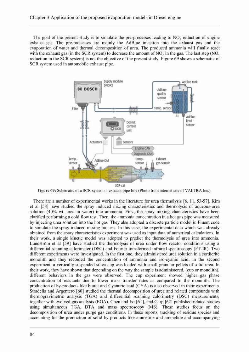
Chapter 3 Application of the proposed evaporation models in Diesel engine
84
The goal of the present study is to simulate the pre-processes leading to NOx reduction of engine exhaust gas. The pre-processes are mainly the AdBlue injection into the exhaust gas and the evaporation of water and thermal decomposition of urea. The produced ammonia will finally react with the exhaust gas (in the SCR system) to decrease the amount of NOx in the gas. The last step (NOx reduction in the SCR system) is not the objective of the present study. Figure 69 shows a schematic of SCR system used in automobile exhaust pipe.
Figure 69: Schematic of a SCR system in exhaust pipe line (Photo from internet site of VALTRA Inc.).
There are a number of experimental works in the literature for urea thermolysis [6, 11, 53-57]. Kim et al [58] have studied the spray induced mixing characteristics and thermolysis of aqueous-urea solution (40% wt. urea in water) into ammonia. First, the spray mixing characteristics have been clarified performing a cold flow test. Then, the ammonia concentration in a hot gas pipe was measured by injecting urea solution into the hot gas. They also adopted a discrete particle model in Fluent code to simulate the spray-induced mixing process. In this case, the experimental data which was already obtained from the spray characteristics experiment was used as input data of numerical calculations. In their work, a single kinetic model was adopted to predict the thermolysis of urea into ammonia. Lundström et al [59] have studied the thermolysis of urea under flow reactor conditions using a differential scanning calorimeter (DSC) and Fourier transformed infrared spectroscopy (FT-IR). Two different experiments were investigated. In the first one, they administered urea solution in a cordierite monolith and they recorded the concentration of ammonia and iso-cyanic acid. In the second experiment, a vertically suspended silica cup was loaded with small granular pellets of solid urea. In their work, they have shown that depending on the way the sample is administered, (cup or monolith), different behaviors in the gas were observed. The cup experiment showed higher gas phase concentration of reactants due to lower mass transfer rates as compared to the monolith. The production of by-products like biuret and Cyanuric acid (CYA) is also observed in their experiments. Stradella and Argentero [60] studied the thermal decomposition of urea and related compounds with thermogravimetric analysis (TGA) and differential scanning calorimetry (DSC) measurements, together with evolved gas analysis (EGA). Chen and Isa [61], and Carp [62] published related studies using simultaneous TGA, DTA and mass spectroscopy (MS). These studies focus on the decomposition of urea under purge gas conditions. In these reports, tracking of residue species and accounting for the production of solid by-products like ammeline and ammelide and accompanying
Development of multi-component evaporation models and 3D modeling of NOx-SCR reduction system
85
synthetic details were not included. Schaber et al [63] studied the thermal decomposition of urea under open reaction vessel conditions by thermogravimetric analysis (TGA), high performance liquid chromatography (HPLC), Fourier transform-infrared (FT-IR) and an ammonium ion-selective electrode (ISE). Evolved gases and urea were analyzed and profiles of substances obtained from different reactions of urea thermolysis (i.e. biuret, cyanuric acid (CYA), ammelide, ammeline and melamine) versus temperature were given. In their work, major reaction intermediates are identified and production of biuret, cyanuric acid, ammelide, ammeline and melamine as a function of temperature were investigated. They also showed that in the thermolysis process, to complete a reaction, the temperature should be high enough. Numerical modeling of urea thermolysis for SCR systems has recently been conducted. Analyzing the literature, several studies on the evaporation and thermolysis of urea-water-solution from sprayed droplets can be found, e.g. [13, 15, 66-69, 182]. Munnannur and Liu [65] developed a multi-dimensional model to describe key non-catalytic processes that occur during the conversion of Diesel Exhaust Fluid (DEF) into ammonia in SCR systems. Birkhold et al. [15] developed a 3D numerical model of injection of urea-water solution. They considered the interaction of the spray with both the hot gas stream and walls of the exhaust pipe. In a complementary work [13] Birkhold et al. developed a thermolysis model for urea particles based on the experimental data of Kim et al. [58]. In their work, thermal decomposition of urea was limited to the molten urea. In addition, they did not account for the production of by-products like biuret, ammeline and ammelide. In the present study, a model for thermal decomposition of urea is developed based on the experiments of Lundström et al. [59] and Schaber et al. [63]. In addition to the thermolysis of urea, the new model takes into account the thermal decomposition of by-products (biuret, cyanuric acid-CYA and ammelide). The kinetic model considers also the hydrolysis of water in the UWS particles. Ammonia production from UWS contains physical and chemical processes. Water evaporates from UWS particles and solid/liquid urea decomposes into ammonia and other chemical species. There is no clear understanding about the physical state of urea during the evaporation and thermolysis processes. Surveying the literature, different physical states of urea during thermal decomposition could be found [13, 54]. But, the dominant hypothesis is that thermal decomposition of urea starts after the end of water evaporation. In this case, solid urea first melts and then decomposes into ammonia and iso-cyanic acid and eventually other components [13, 57, 65, 69, 176]. In order to be able to simulate the ammonia production and eventually the urea and by-products deposition inside the exhaust pipe from UWS, a study of evaporation and thermolysis of UWS is performed in the next chapters. In Chapter 4 an evaporation model for UWS is proposed. The multi-component evaporation models presented in part 1 of this manuscript have been improved in this work in order to take into account the effect of dissolved urea on the evaporation of water. Indeed, a NRTL (Non-Random Two Liquids) activity model is used to predict the vapor pressure of UWS. The vapor pressure of urea is very low compared to that of water. The evaporation of water leads to a progressive increase in the concentration of urea in the UWS. This process is explained in detail in Chapter 4. In addition, it is assumed that the thermolysis of aqueous-urea starts at the beginning of the evaporation process. A set of chemical reactions containing aqueous/solid urea and by-products thermolysis is used in the thermolysis model proposed in Chapter 5. The evaporation and thermolysis models are presented in Chapter 4 and Chapter 5 and used to simulate the experiment of Lundström et al. [59] for solid urea and UWS thermolysis cases. For the thermolysis of UWS, the evaporation model is coupled to the thermolysis model. Both evaporation and thermolysis models are then used to simulate the experiment of Kim et al. [58]. The application of the evaporation and thermolysis models in a typical SCR system is finally presented in Chapter 6.
Chapter 4
Evaporation model for urea-water solution 4.1 Introduction Evaporation phenomenon for hydrocarbon mixtures has been completely described in the previous chapters. However, evaporation of Urea-Water Solution (UWS) is a little more complicated due to the interaction of urea solute in the water. When injected to the exhaust hot gas, UWS droplets undergo heating which leads to a progressive increase of urea concentration inside the droplet during the water evaporation process. The effects of solute on evaporation of droplets have been studied by Basu and Cetegen [183]. They modeled liquid ceramic precursor droplets (composed of water and zirconium acetate) axially injected into plasma. As water evaporates, the concentration of solute increases, which leads to the formation of a precipitate shell. They studied the effects of droplet size, shell porosity and thickness and they shown different behavior of droplet for different conditions. The same hypothesis may be applied to the UWS droplets. Dissolved urea affects the evaporation of water directly. As the urea evaporation rate is very small relatively to water, the concentration of urea in the droplet increases. Two different scenarios may happen for the urea depending on the rapidity of the water evaporation. When the droplet size is small and/or the vaporization of water is slow, the concentration of urea throughout the droplet increases uniformly which finally leads to the formation of a solid particle. But, when rapid water vaporization occurs on the droplet surface, urea concentration increases at the droplet surface which builds up a urea shell around the droplet. This may lead to the boiling of the water inside the urea shell and even to the explosion and fragmentation of the droplet as it has been observed by [184]. Although, the last scenario may occur for large droplets with high heating rate, it will not be considered in the present work. In the suggested UWS evaporation model presented in this chapter, dissolved urea inside or at the droplet surface causes the vapor pressure of water to decrease which consequently decreases the evaporation rate of water in UWS compared to pure water. Some authors [13, 14] have considered the effect of urea on water vapor pressure. Birkhold et al. [13] used Rapid Mixing model (RM model) to evaluate the influence of dissolved urea on the evaporation of water. In the RM model, infinite high transport coefficients are assumed for the liquid phase, resulting in spatial uniform temperature, concentration and fluid properties in the droplet, with the temporal change in quantities [13, 185, 186]. Kontin et al. [14] used the RM model (like Birkhold et al. [13]) for evaporation of water in UWS. They modified the standard gaseous-film model, proposed by Abramzon & Sirignano [16], by introducing the mass flow reduction coefficient proposed by Reinhold [187]. They proposed three different cases during the evaporation of water and enrichment of urea: in the oversaturated case, urea completely remains in solution, therefore an unlimited oversaturation is assumed to be possible. In the saturated case, a limited solubility is
Development of multi-component evaporation models and 3D modeling of NOx-SCR reduction system
87
considered by precipitation of solid crystalline urea out of the liquid phase. The saturation pressure is influenced in this case according to Raoult's law. In the crust case, a solid layer is formed at the particle surface during dissolution/evaporation which reduces the mass transfer. A reduction coefficient is then introduced in the evaporation rate expression and adjusted in their study, using an experimental investigation. This model gives relatively good results. However, an exact physical explanation for the reduction coefficient is necessary. In the present work, a droplet evaporation model is proposed, based on the multi-component droplet evaporation model developed by the authors [145] and described in Chapter 1, which takes into account a modified Stephan velocity and enthalpy diffusion of gaseous species to compute the evaporation rate. The mass conservation equation of gas mixture is conserved by diffusive mass flux which is commonly approximated by Fick's law for binary mixtures. The model uses spherical droplet hypothesis with no interaction between droplets. The effects of radiation, Soret and Dufour are neglected. The one-third rule is used for the properties of the gaseous mixture in the film region around the droplet [128]. Gas phase quasi-steadiness and isobaric assumptions are applied to the model. The droplet temperature is assumed to be uniform during all the process of evaporation (i.e., the infinite thermal conductivity assumption is invoked). The resulting governing equations for the model consist in the two phase flow equations for the gas and liquid phases along with the thermodynamic equilibrium condition at the liquid-gas interface. Although the urea-water droplets contain two individual components (i.e., water and urea) and needs a two-component evaporation model, the evaporation rate of urea especially for the exhaust system conditions (i.e. more or less atmospheric pressure) is negligible compared to the evaporation rate of water. This feature is due to the very low vapor pressure of urea at atmospheric pressure. Therefore, the two-component evaporation model has been simplified as follows: only water is evaporated using the Single-component evaporation model (see Chapter 1) where the UWS vapor pressure is obtained using the Raoult's law by the aid of the NRTL (Non-Random Two-Liquids) activity model [52]. The NRTL model is also integrated in the liquid film evaporation model developed in Chapter 2 of the present manuscript in the same manner as droplet evaporation. Thus, only the evaporation of UWS droplet will be presented here. 4.2 UWS evaporation model The UWS evaporation model is described in this section including some details of the activity calculations using the NRTL model. It will be referred bellow as UWS-NRTL. For completeness, some equations already given in Chapter 1 are recalled in the following sections. 4.2.1 Gas phase governing equations Droplet evaporation models are generally based on the conservation equations of mass, momentum and energy. In the resolving of the mass conservation equation of species, it is assumed that there is no chemical reaction in the gaseous environment. This is a good assumption for urea and water species. There is almost no urea vapor in the gaseous environment due to its very low evaporation rate. Besides, the reactions of gaseous species with water vapor are negligible at low temperatures [188-190]. The gas phase governing equations are used to obtain the mass flow rate and heat flux from the gas to the liquid. These quantities for water evaporation are summarized in the following sections. 4.2.2 Mass flow rate Based on the previous works, some authors [16, 25] have considered the gaseous boundary layer around the droplet to evaluate heat and mass fluxes. These models give the instantaneous droplet vaporization rate from the integration of the quasi-steady species balance around the droplet. The mass evaporation rate for single-component water droplet, drawn from multi-component evaporation rate, (Equation (1.31)), is presented as:
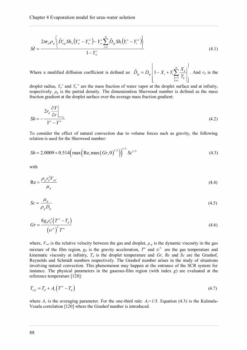
Chapter 4 Evaporation model for urea-water solution
88
s
w
N
ii
siiig
sww
sww
swggd
Y
YYShDYYYShDrM
1
ˆˆ21
(4.1)
Where a modified diffusion coefficient is defined as: 1
ˆ 1N
kig ig i i
k kk i
XD D X YY
. And rd is the
droplet radius, Yws and Yw
∞ are the mass fraction of water vapor at the droplet surface and at infinity, respectively. ρg is the partial density. The dimensionless Sherwood number is defined as the mass fraction gradient at the droplet surface over the average mass fraction gradient:
2d
dr r
s
Yrr
ShY Y
(4.2)
To consider the effect of natural convection due to volume forces such as gravity, the following relation is used for the Sherwood number:
1/ 21/ 2 1/32.0009 0.514 max Re,max ,0Sh Gr Sc (4.3)
with
2
Re g d rel
g
r V
(4.4)
g
g g
ScD
(4.5)
30
2
8 d dg r T TGr
T
(4.6)
where, Vrel is the relative velocity between the gas and droplet, μ,g is the dynamic viscosity in the gas mixture of the film region, g0 is the gravity acceleration, T∞ and are the gas temperature and kinematic viscosity at infinity, Td is the droplet temperature and Gr, Re and Sc are the Grashof, Reynolds and Schmidt numbers respectively. The Grashof number arises in the study of situations involving natural convection. This phenomenon may happen at the entrance of the SCR system for instance. The physical parameters in the gaseous-film region (with index g) are evaluated at the reference temperature [128]:
ref d r dT T A T T (4.7) where Ar is the averaging parameter. For the one-third rule: Ar=1/3. Equation (4.3) is the Kulmala-Vesala correlation [120] where the Grashof number is introduced.
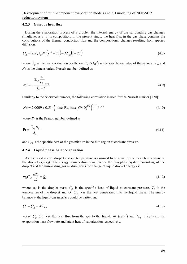
Development of multi-component evaporation models and 3D modeling of NOx-SCR reduction system
89
4.2.3 Gaseous heat flux During the evaporation process of a droplet, the internal energy of the surrounding gas changes simultaneously to its composition. In the present study, the heat flux in the gas phase contains the contributions of the thermal conduction flux and the compositional changes resulting from species diffusion:
swgdgdg YhMTTNurQ 12 (4.8)
where g is the heat conduction coefficient, hg (J.kg-1) is the specific enthalpy of the vapor at Tref and Nu is the dimensionless Nusselt number defined as:
2d
dr r
d
Trr
NuT T
(4.9)
Similarly to the Sherwood number, the following correlation is used for the Nusselt number [120]:
1/ 21/ 2 1/32.0009 0.514 max Re,max ,0 PrNu Gr (4.10)
where Pr is the Prandtl number defined as:
Pr pg g
g
C
(4.11)
and Cpg is the specific heat of the gas mixture in the film region at constant pressure. 4.2.4 Liquid phase balance equation As discussed above, droplet surface temperature is assumed to be equal to the mean temperature of the droplet (Ts=Td). The energy conservation equation for the two phase system consisting of the droplet and the surrounding gas mixture gives the change of liquid droplet energy as:
dd pf l
dTm C Qdt
(4.12)
where md is the droplet mass, Cpf is the specific heat of liquid at constant pressure, Td is the temperature of the droplet and lQ (J.s-1) is the heat penetrating into the liquid phase. The energy balance at the liquid-gas interface could be written as:
gvgl LMQQ , (4.13)
where gQ (J.s-1) is the heat flux from the gas to the liquid. m (kg.s-1) and ,v gL (J.kg-1) are the evaporation mass flow rate and latent heat of vaporization respectively.
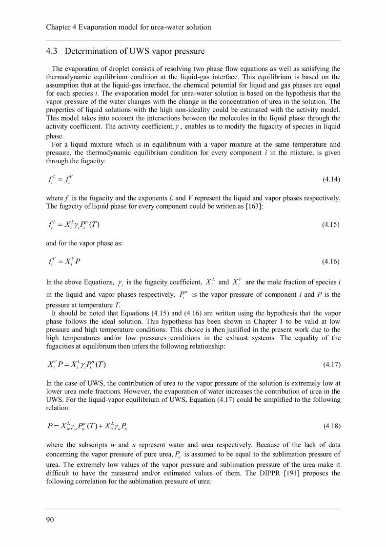
Chapter 4 Evaporation model for urea-water solution
90
4.3 Determination of UWS vapor pressure The evaporation of droplet consists of resolving two phase flow equations as well as satisfying the thermodynamic equilibrium condition at the liquid-gas interface. This equilibrium is based on the assumption that at the liquid-gas interface, the chemical potential for liquid and gas phases are equal for each species i. The evaporation model for urea-water solution is based on the hypothesis that the vapor pressure of the water changes with the change in the concentration of urea in the solution. The properties of liquid solutions with the high non-ideality could be estimated with the activity model. This model takes into account the interactions between the molecules in the liquid phase through the activity coefficient. The activity coefficient, , enables us to modify the fugacity of species in liquid phase. For a liquid mixture which is in equilibrium with a vapor mixture at the same temperature and pressure, the thermodynamic equilibrium condition for every component i in the mixture, is given through the fugacity:
L Vi if f (4.14)
where f is the fugacity and the exponents L and V represent the liquid and vapor phases respectively. The fugacity of liquid phase for every component could be written as [163]:
( )L Li i i if X P T (4.15)
and for the vapor phase as:
V Vi if X P (4.16)
In the above Equations, i is the fugacity coefficient, L
iX and ViX are the mole fraction of species i
in the liquid and vapor phases respectively. iP is the vapor pressure of component i and P is the pressure at temperature T. It should be noted that Equations (4.15) and (4.16) are written using the hypothesis that the vapor phase follows the ideal solution. This hypothesis has been shown in Chapter 1 to be valid at low pressure and high temperature conditions. This choice is then justified in the present work due to the high temperatures and/or low pressures conditions in the exhaust systems. The equality of the fugacities at equilibrium then infers the following relationship:
( )V Li i i iX P X P T (4.17)
In the case of UWS, the contribution of urea to the vapor pressure of the solution is extremely low at lower urea mole fractions. However, the evaporation of water increases the contribution of urea in the UWS. For the liquid-vapor equilibrium of UWS, Equation (4.17) could be simplified to the following relation:
( )L Lw w w u u uP X P T X P (4.18)
where the subscripts w and u represent water and urea respectively. Because of the lack of data concerning the vapor pressure of pure urea, uP is assumed to be equal to the sublimation pressure of urea. The extremely low values of the vapor pressure and sublimation pressure of the urea make it difficult to have the measured and/or estimated values of them. The DIPPR [191] proposes the following correlation for the sublimation pressure of urea:
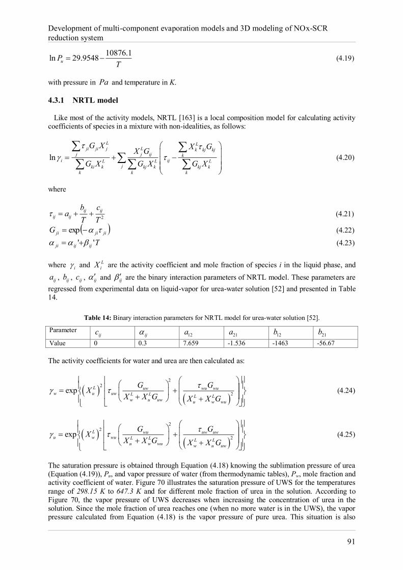
Development of multi-component evaporation models and 3D modeling of NOx-SCR reduction system
91
10876.1ln 29.9548uPT
(4.19)
with pressure in Pa and temperature in K. 4.3.1 NRTL model Like most of the activity models, NRTL [163] is a local composition model for calculating activity coefficients of species in a mixture with non-idealities, as follows:
ln
L LLji ji j k kj kj
j j ij ki ijL L L
jki k kj k kj kk k k
G X X GX GG X G X G X
(4.20)
where
2ij ij
ij ij
b ca
T T (4.21)
jijijiG exp (4.22)
Tijijji '' (4.23) where i and L
iX are the activity coefficient and mole fraction of species i in the liquid phase, and
ija , ijb , ijc , ij and ij are the binary interaction parameters of NRTL model. These parameters are regressed from experimental data on liquid-vapor for urea-water solution [52] and presented in Table 14.
Table 14: Binary interaction parameters for NRTL model for urea-water solution [52].
Parameter ijc ij 12a 21a 12b 21b
Value 0 0.3 7.659 -1.536 -1463 -56.67 The activity coefficients for water and urea are then calculated as:
22
2exp L uw wu wuw u uw L L L L
w u uw u w wu
G GXX X G X X G
(4.24)
22
2exp L wu uw uwu w wu L L L L
u w wu w u uw
G GXX X G X X G
(4.25)
The saturation pressure is obtained through Equation (4.18) knowing the sublimation pressure of urea (Equation (4.19)), Pu, and vapor pressure of water (from thermodynamic tables), Pw, mole fraction and activity coefficient of water. Figure 70 illustrates the saturation pressure of UWS for the temperatures range of 298.15 K to 647.3 K and for different mole fraction of urea in the solution. According to Figure 70, the vapor pressure of UWS decreases when increasing the concentration of urea in the solution. Since the mole fraction of urea reaches one (when no more water is in the UWS), the vapor pressure calculated from Equation (4.18) is the vapor pressure of pure urea. This situation is also
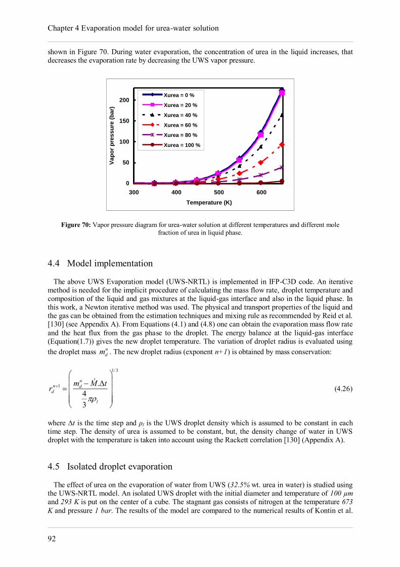
Chapter 4 Evaporation model for urea-water solution
92
shown in Figure 70. During water evaporation, the concentration of urea in the liquid increases, that decreases the evaporation rate by decreasing the UWS vapor pressure.
0
50
100
150
200
300 400 500 600
Temperature (K)
Va
po
r p
res
su
re (
ba
r)
Xurea = 0 %
Xurea = 20 %
Xurea = 40 %
Xurea = 60 %
Xurea = 80 %
Xurea = 100 %
Figure 70: Vapor pressure diagram for urea-water solution at different temperatures and different mole fraction of urea in liquid phase.
4.4 Model implementation The above UWS Evaporation model (UWS-NRTL) is implemented in IFP-C3D code. An iterative method is needed for the implicit procedure of calculating the mass flow rate, droplet temperature and composition of the liquid and gas mixtures at the liquid-gas interface and also in the liquid phase. In this work, a Newton iterative method was used. The physical and transport properties of the liquid and the gas can be obtained from the estimation techniques and mixing rule as recommended by Reid et al. [130] (see Appendix A). From Equations (4.1) and (4.8) one can obtain the evaporation mass flow rate and the heat flux from the gas phase to the droplet. The energy balance at the liquid-gas interface (Equation(1.7)) gives the new droplet temperature. The variation of droplet radius is evaluated using the droplet mass n
dm . The new droplet radius (exponent n+1) is obtained by mass conservation:
1/3
1 .43
nn d
d
l
m M tr
(4.26)
where ∆t is the time step and ρl is the UWS droplet density which is assumed to be constant in each time step. The density of urea is assumed to be constant, but, the density change of water in UWS droplet with the temperature is taken into account using the Rackett correlation [130] (Appendix A). 4.5 Isolated droplet evaporation The effect of urea on the evaporation of water from UWS (32.5% wt. urea in water) is studied using the UWS-NRTL model. An isolated UWS droplet with the initial diameter and temperature of 100 µm and 293 K is put on the center of a cube. The stagnant gas consists of nitrogen at the temperature 673 K and pressure 1 bar. The results of the model are compared to the numerical results of Kontin et al.
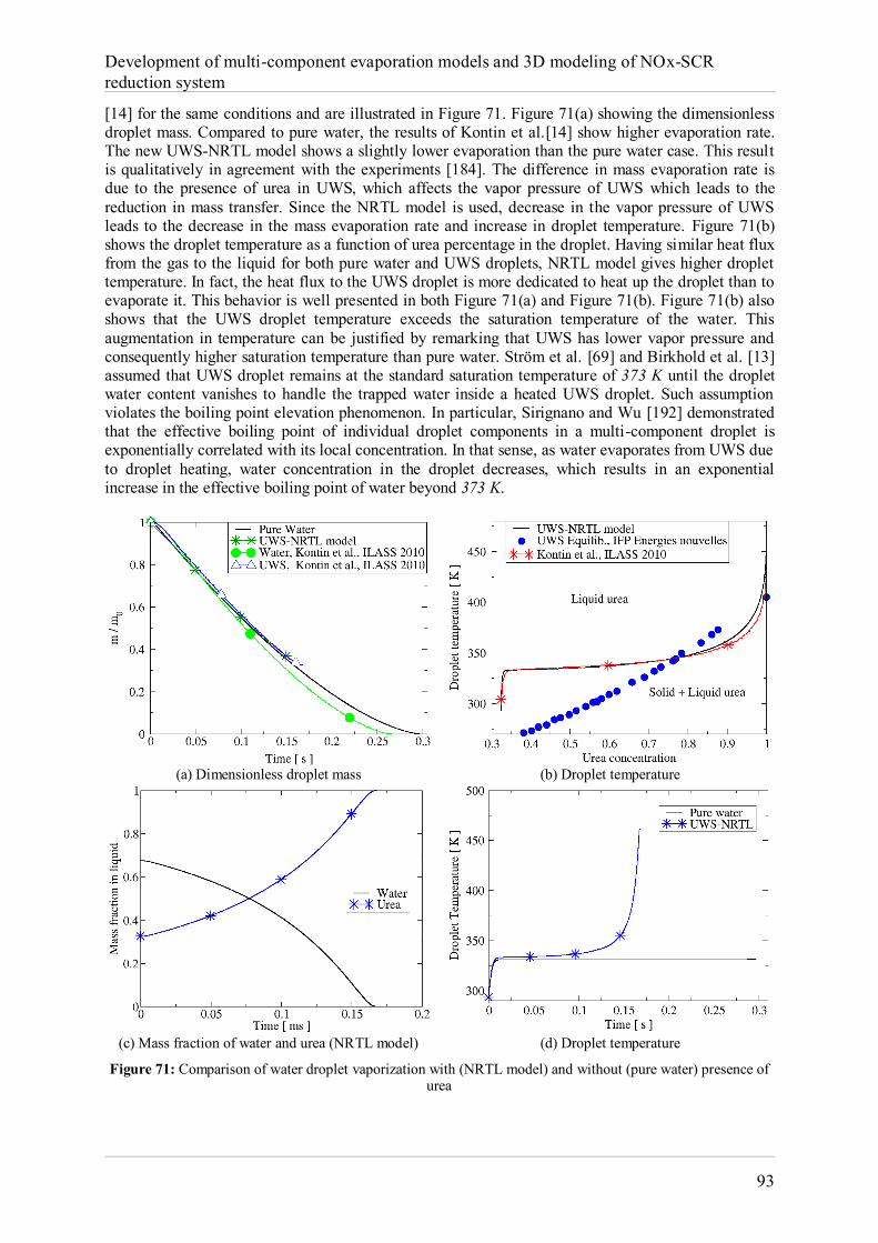
Development of multi-component evaporation models and 3D modeling of NOx-SCR reduction system
93
[14] for the same conditions and are illustrated in Figure 71. Figure 71(a) showing the dimensionless droplet mass. Compared to pure water, the results of Kontin et al.[14] show higher evaporation rate. The new UWS-NRTL model shows a slightly lower evaporation than the pure water case. This result is qualitatively in agreement with the experiments [184]. The difference in mass evaporation rate is due to the presence of urea in UWS, which affects the vapor pressure of UWS which leads to the reduction in mass transfer. Since the NRTL model is used, decrease in the vapor pressure of UWS leads to the decrease in the mass evaporation rate and increase in droplet temperature. Figure 71(b) shows the droplet temperature as a function of urea percentage in the droplet. Having similar heat flux from the gas to the liquid for both pure water and UWS droplets, NRTL model gives higher droplet temperature. In fact, the heat flux to the UWS droplet is more dedicated to heat up the droplet than to evaporate it. This behavior is well presented in both Figure 71(a) and Figure 71(b). Figure 71(b) also shows that the UWS droplet temperature exceeds the saturation temperature of the water. This augmentation in temperature can be justified by remarking that UWS has lower vapor pressure and consequently higher saturation temperature than pure water. Ström et al. [69] and Birkhold et al. [13] assumed that UWS droplet remains at the standard saturation temperature of 373 K until the droplet water content vanishes to handle the trapped water inside a heated UWS droplet. Such assumption violates the boiling point elevation phenomenon. In particular, Sirignano and Wu [192] demonstrated that the effective boiling point of individual droplet components in a multi-component droplet is exponentially correlated with its local concentration. In that sense, as water evaporates from UWS due to droplet heating, water concentration in the droplet decreases, which results in an exponential increase in the effective boiling point of water beyond 373 K.
(a) Dimensionless droplet mass (b) Droplet temperature
(c) Mass fraction of water and urea (NRTL model) (d) Droplet temperature
Figure 71: Comparison of water droplet vaporization with (NRTL model) and without (pure water) presence of urea
Chapter 4 Evaporation model for urea-water solution
94
The mass fraction of water and urea in UWS droplet is shown in Figure 71(c). Since water evaporates from UWS droplet, its contribution in droplet decreases (Figure 71(c)). The saturation temperature of the UWS then increases by increasing the urea percentage in UWS. According to Figure 71(d), the UWS-NRTL model increases the droplet temperature compared to the pure water. The effect of urea on UWS droplets temperature (Figure 71(d)) seems to be more important that its effect on water evaporation (Figure 71(a)). Since the thermolysis of urea is highly related to the droplet temperature, an incorrect value of temperature may lead to the uncertainties in the thermolysis phenomenon. Hence, the UWS-NRTL model helps to accurately calculate the droplet temperature to be used in the thermal decomposition of urea. According to Figure 71(a), water evaporation from UWS continues until it reaches the 32.5% of the droplet mass. The rest of the mass in UWS droplet is assumed to be the mass of solid/molten urea. 4.6 Conclusions In the present study, an UWS evaporation model has been suggested. This model differs from the multi-component droplets evaporation model described in Chapter 1. Indeed, it takes into account the effects of dissolved urea on evaporation model. The vapor pressure of urea-water solution which has an important effect on the evaporation rate is obtained from the Raoult's law using the NRTL activity model. The results of the evaporation model with and without considering the effect of urea on evaporation rate show a small effect on the water evaporation but a significant effect of UWS temperature especially near the end of the water evaporation. The proposed UWS-NRTL model will be used for the SCR simulation in Chapter 6.
Chapter 5
Urea thermal decomposition modeling 5.1 Introduction Selective Catalytic Reduction (SCR) is one of the most promising techniques for the abatement of the nitrogen oxides (NOx) emissions from lean-burn engines. For reasons of safety and toxicity, urea is the preferred selective reducing agent for mobile SCR applications [176, 193]. Urea is typically being used as an aqueous solution at its eutectic composition (32.5%wt urea, marketed as Adblue®). In a typical SCR system, urea-water-solution (UWS) is sprayed into the hot engine exhaust upstream of the SCR catalyst. It is commonly believed that water evaporates first [13] and the remaining solid urea then melts and decomposes into gas phase ammonia (NH3) and isocyanic acid (HNCO) and eventually other by-products [13, 57, 65, 69, 176]. However, urea decomposition in aqueous solution occurs in the same temperature range as water evaporation [55]. In Chapter 4, it was shown how UWS droplets or liquid film undergo heating and water vaporization leading to high urea concentration near droplet or film surface. Dissolved urea at the droplet surface causes the vapor pressure of water to decrease which consequently decreases the evaporation rate of water in UWS compared to the pure water [13, 14, 194]. In the same time, urea decomposes through thermolysis. Several computational studies were carried out to predict UWS thermolysis. Abu-Ramadan et al. [182] studied the evaporation and thermolysis of UWS droplets. They modeled urea depletion from UWS either as a vaporization process or a direct thermolysis process from molten urea to ammonia and isocyanic acid. The formation of by-products (biuret and higher molecular complexes) was neglected in their study. Birkhold et al. [13] found the rapid mixing model (as used in our models described in Chapter 1) to have the best trade-off between accuracy and numerical effort. However, these studies did not consider the formation of deposits resulting from urea decomposition. Deposit formation can lead to pressure lost, deterioration of the after-treatment system [70] and possible deactivation of the SCR catalyst [195]. In the present chapter, some characteristics of urea and Adblue are provided together with a brief introduction on chemical reaction and thermal decomposition definitions. Then, general methodologies for SCR system, used in the literature, are discussed. Single-step thermolysis models for urea in different physical states, suggested in the literature, are presented. Finally, a new multi-step thermolysis model is proposed and validated against experimental data.
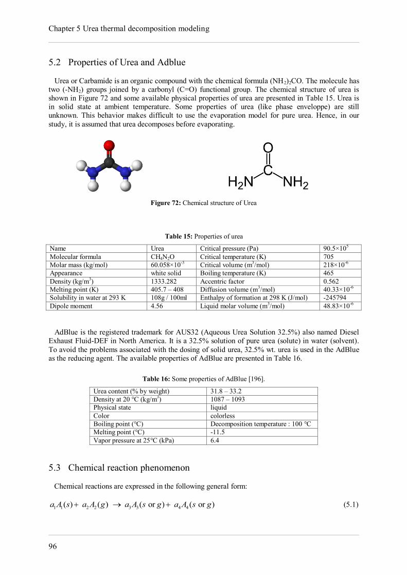
Chapter 5 Urea thermal decomposition modeling
96
5.2 Properties of Urea and Adblue Urea or Carbamide is an organic compound with the chemical formula (NH2)2CO. The molecule has two (-NH2) groups joined by a carbonyl (C=O) functional group. The chemical structure of urea is shown in Figure 72 and some available physical properties of urea are presented in Table 15. Urea is in solid state at ambient temperature. Some properties of urea (like phase enveloppe) are still unknown. This behavior makes difficult to use the evaporation model for pure urea. Hence, in our study, it is assumed that urea decomposes before evaporating.
Figure 72: Chemical structure of Urea
Table 15: Properties of urea
Name Urea Critical pressure (Pa) 90.5×10⁵ Molecular formula CH4N2O Critical temperature (K) 705 Molar mass (kg/mol) 60.058×10⁻³ Critical volume (m3/mol) 218×10-6 Appearance white solid Boiling temperature (K) 465 Density (kg/m3) 1333.282 Accentric factor 0.562 Melting point (K) 405.7 – 408 Diffusion volume (m3/mol) 40.33×10⁻⁶ Solubility in water at 293 K 108g / 100ml Enthalpy of formation at 298 K (J/mol) -245794 Dipole moment 4.56 Liquid molar volume (m3/mol) 48.83×10⁻⁶ AdBlue is the registered trademark for AUS32 (Aqueous Urea Solution 32.5%) also named Diesel Exhaust Fluid-DEF in North America. It is a 32.5% solution of pure urea (solute) in water (solvent). To avoid the problems associated with the dosing of solid urea, 32.5% wt. urea is used in the AdBlue as the reducing agent. The available properties of AdBlue are presented in Table 16.
Table 16: Some properties of AdBlue [196].
Urea content (% by weight) 31.8 – 33.2 Density at 20 °C (kg/m3) 1087 – 1093 Physical state liquid Color colorless Boiling point (°C) Decomposition temperature : 100 °C Melting point (°C) -11.5 Vapor pressure at 25°C (kPa) 6.4
5.3 Chemical reaction phenomenon Chemical reactions are expressed in the following general form:
1 1 2 2 3 3 4 4( ) ( ) ( or ) ( or )a A s a A g a A s g a A s g (5.1)
Development of multi-component evaporation models and 3D modeling of NOx-SCR reduction system
97
where A1 and A2 are the reactants and A3 and A4 are the products of the reaction. The general reaction rate for an elementary reaction (like Equation (5.1)) can be obtained using Eyring expression:
1 2
1 2
rGa areaction RTBk Tr e A A
h
(5.2)
where reactionr is the rate constant, kB is the Boltzmann constant, h the Planck constant, rG is the gibbs energy of the activated complex and T is the temperature. Rates of reaction depend basically on:
Reactant concentrations, which usually make the reaction to happen at a faster rate if raised through increased collisions per unit time.
Pressure, which decreases the distance between the molecules when increasing. Activation energy, defined as the amount of energy required to make the reaction start and
carry on spontaneously. Higher activation energy means that the reactants need more energy to start reacting.
Temperature, which increases the energy of the molecules and creates more collisions per unit time when increasing.
The presence or absence of a catalyst. 5.4 Thermal decomposition definition Thermal decomposition, or thermolysis, is a chemical decomposition caused by heat. The reaction is usually endothermic as heat is required to break chemical bonds in the compound undergoing decomposition. In this study, the rate of a chemical reaction is taken in the Arrhenius form that can be expressed as [197]:
exp /ak A E RT (5.3) where k is the rate constant, A is the frequency factor, Ea is the activation energy, R is the gas constant and T is the temperature. In the next Sections, thermal decomposition of urea in the three physical states (i.e., gas, liquid and solid) is described. 5.5 SCR system modeling from literatures The SCR system uses ammonia to react with NOx in the exhaust gas of Diesel engines in the presence of a catalyst or oxygen. The reaction is represented in different forms regarding to different engine and exhaust gas conditions [198]:
3 2 2 2 24 4 3 4 6 2NH NO O N H O O (5.4)
OHNNONONH 2223 64224 (5.5)
OHNONONH 22223 6324 (5.6) The result of the reaction is water and nitrogen. As discussed, to provide the ammonia needed for SCR system, AdBlue is injected to the exhaust gas; water evaporates from AdBlue and urea decomposes
Chapter 5 Urea thermal decomposition modeling
98
into ammonia. An example of the properties of burnt gas in the exhaust pipe line and the injected spray are given in Table 17 [13]. They vary for different engines and operating conditions.
Table 17: Burnt gas and spray properties [13].
Exhaust
Gas velocity (m/s) 5 – 40 Gas Temperature (K) 400 – 1000 Pressure (bar) 1 Wall temperature (K) 350 – 900
Spray (AdBlue)
SMD (µm) 20 – 150 Injection velocity (m/s) 5 – 25 Initial spray temperature (K) 300 – 350
The result of urea thermolysis is ammonia, iso-cyanic acid and other chemical species according to different conditions, as described by the following global reaction:
22 32
or or HCO NH s l g NH g HNCO g (5.7)
Then, iso-cyanic may hydrolyse to ammonia and carbon dioxide:
32 3 2
HHNCO g H O g NH g CO g (5.8)
This will be addressed later in Section 5.7. In Equations (5.7) and (5.8), 2H and 3H are the reaction enthalpies. It has been widely accepted that the above processes take place as the urea-water-solution is injected into hot exhaust gas [6, 176]. The overall urea decomposition reaction corresponds to the two-steps:
42 2 3 22
or or 2HCO NH s l g H O NH g CO g (5.9)
The above reaction is called thermo-hydrolysis as it includes the hydrolysis of iso-cyanic acid. Different processes for urea thermolysis have been indicated at different temperatures in the literature. In particular, some byproducts like biuret, cyanuric acid, ammelide, ammeline and other compounds of high molecular weight may be formed [53, 63, 199]. When urea is heated very quickliy, only the two-step reactions of urea thermolysis (Equation (5.7)) and hydrolysis (Equation (5.8)) may be considered as the production of by-products (i.e., biuret, cyanuric acid, etc.) is avoided [11]. In the following section, single-step models of thermal decomposition of urea, found in the literature, are presented. 5.6 Single-step thermolysis models The chemical reaction for the urea thermolysis (Equation (5.7)) is identical for the three forms of urea (solid, liquid or gas), but the decomposition rates are different as shown bellow.
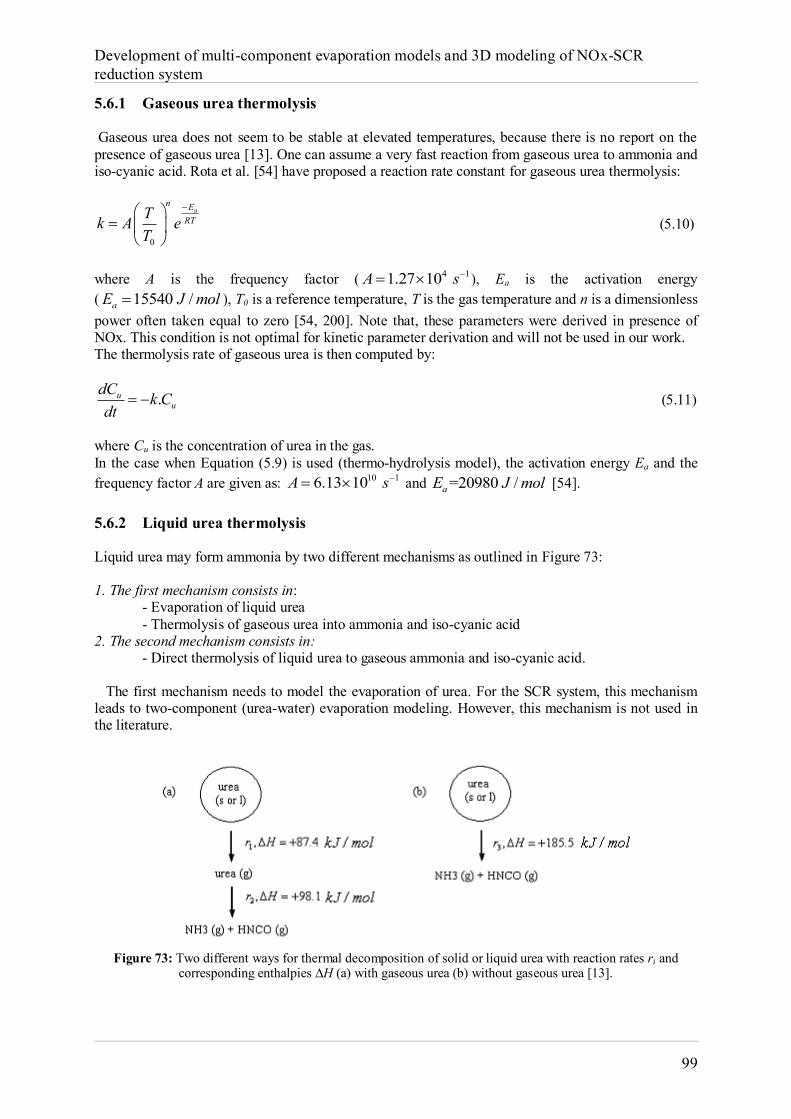
Development of multi-component evaporation models and 3D modeling of NOx-SCR reduction system
99
5.6.1 Gaseous urea thermolysis Gaseous urea does not seem to be stable at elevated temperatures, because there is no report on the presence of gaseous urea [13]. One can assume a very fast reaction from gaseous urea to ammonia and iso-cyanic acid. Rota et al. [54] have proposed a reaction rate constant for gaseous urea thermolysis:
0
an E
RTTk A eT
(5.10)
where A is the frequency factor ( 4 11.27 10 A s ), Ea is the activation energy ( 15540 /aE J mol ), T0 is a reference temperature, T is the gas temperature and n is a dimensionless power often taken equal to zero [54, 200]. Note that, these parameters were derived in presence of NOx. This condition is not optimal for kinetic parameter derivation and will not be used in our work. The thermolysis rate of gaseous urea is then computed by:
.uu
dC k Cdt
(5.11)
where Cu is the concentration of urea in the gas. In the case when Equation (5.9) is used (thermo-hydrolysis model), the activation energy Ea and the frequency factor A are given as: 10 16.13 10 A s and =20980 /aE J mol [54]. 5.6.2 Liquid urea thermolysis Liquid urea may form ammonia by two different mechanisms as outlined in Figure 73: 1. The first mechanism consists in:
- Evaporation of liquid urea - Thermolysis of gaseous urea into ammonia and iso-cyanic acid
2. The second mechanism consists in: - Direct thermolysis of liquid urea to gaseous ammonia and iso-cyanic acid.
The first mechanism needs to model the evaporation of urea. For the SCR system, this mechanism leads to two-component (urea-water) evaporation modeling. However, this mechanism is not used in the literature.
Figure 73: Two different ways for thermal decomposition of solid or liquid urea with reaction rates ri and
corresponding enthalpies ∆H (a) with gaseous urea (b) without gaseous urea [13].
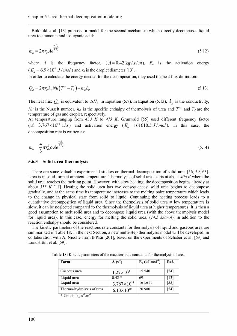
Chapter 5 Urea thermal decomposition modeling
100
Birkhold et al. [13] proposed a model for the second mechanism which directly decomposes liquid urea to ammonia and iso-cyanic acid:
2a
d
ERT
u dm r Ae
(5.12) where A is the frequency factor, ( 0.42 k / /A g s m ), Ea is the activation energy ( 46.9 10 /aE J mol ) and rd is the droplet diameter [13]. In order to calculate the energy needed for the decomposition, they used the heat flux definition:
2d d g d u thQ r Nu T T m h (5.13)
The heat flux dQ is equivalent to 2H in Equation (5.7). In Equation (5.13), g is the conductivity,
Nu is the Nusselt number, hth is the specific enthalpy of thermolysis of urea and T and Td are the temperature of gas and droplet, respectively. At temperature ranging from 433 K to 475 K, Grünwald [55] used different frequency factor ( 143.767 10 1/A s ) and activation energy ( 161610.5 /aE J mol ). In this case, the decomposition rate is written as:
343
a
d
ERT
u dm r Ae
(5.14)
5.6.3 Solid urea thermolysis There are some valuable experimental studies on thermal decomposition of solid urea [56, 59, 63]. Urea is in solid form at ambient temperature. Thermolysis of solid urea starts at about 406 K where the solid urea reaches the melting point. However, with slow heating, the decomposition begins already at about 353 K [11]. Heating the solid urea has two consequences; solid urea begins to decompose gradually, and at the same time its temperature increases to the melting point temperature which leads to the change in physical state from solid to liquid. Continuing the heating process leads to a quantitative decomposition of liquid urea. Since the thermolysis of solid urea at low temperatures is slow, it can be neglected compared to the thermolysis of liquid urea at higher temperatures. It is then a good assumption to melt solid urea and to decompose liquid urea (with the above thermolysis model for liquid urea). In this case, energy for melting the solid urea, (14.5 kJ/mol), in addition to the reaction enthalpy should be considered. The kinetic parameters of the reactions rate constants for thermolysis of liquid and gaseous urea are summarized in Table 18. In the next Section, a new multi-step thermolysis model will be developed, in collaboration with A. Nicolle from IFPEn [201], based on the experiments of Schaber et al. [63] and Lundström et al. [59].
Table 18: Kinetic parameters of the reactions rate constants for thermolysis of urea.
Form
A (s-1) Ea (kJ.mol-1) Ref.
Gaseous urea 41.27 10 15.540 [54]
Liquid urea 0.42 * 69 [13] Liquid urea 143.767 10 161.611 [55] Thermo-hydrolysis of urea 106.13 10 20.980 [54]
* Unit is: kg.s-1.m-1
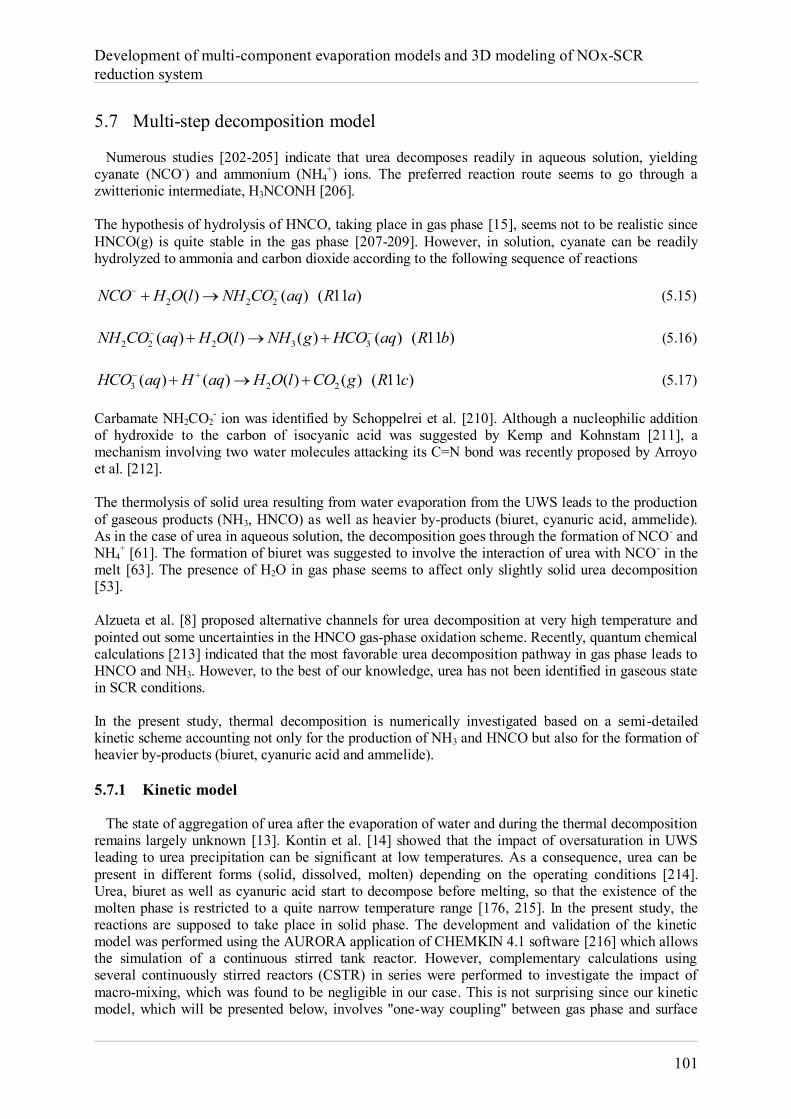
Development of multi-component evaporation models and 3D modeling of NOx-SCR reduction system
101
5.7 Multi-step decomposition model Numerous studies [202-205] indicate that urea decomposes readily in aqueous solution, yielding cyanate (NCO-) and ammonium (NH4
+) ions. The preferred reaction route seems to go through a zwitterionic intermediate, H3NCONH [206]. The hypothesis of hydrolysis of HNCO, taking place in gas phase [15], seems not to be realistic since HNCO(g) is quite stable in the gas phase [207-209]. However, in solution, cyanate can be readily hydrolyzed to ammonia and carbon dioxide according to the following sequence of reactions
2 2 2( ) ( ) ( 11 )NCO H O l NH CO aq R a (5.15)
2 2 2 3 3( ) ( ) ( ) ( ) ( 11 )NH CO aq H O l NH g HCO aq R b (5.16)
3 2 2( ) ( ) ( ) ( ) ( 11 )HCO aq H aq H O l CO g R c (5.17) Carbamate NH2CO2
- ion was identified by Schoppelrei et al. [210]. Although a nucleophilic addition of hydroxide to the carbon of isocyanic acid was suggested by Kemp and Kohnstam [211], a mechanism involving two water molecules attacking its C=N bond was recently proposed by Arroyo et al. [212]. The thermolysis of solid urea resulting from water evaporation from the UWS leads to the production of gaseous products (NH3, HNCO) as well as heavier by-products (biuret, cyanuric acid, ammelide). As in the case of urea in aqueous solution, the decomposition goes through the formation of NCO- and NH4
+ [61]. The formation of biuret was suggested to involve the interaction of urea with NCO- in the melt [63]. The presence of H2O in gas phase seems to affect only slightly solid urea decomposition [53]. Alzueta et al. [8] proposed alternative channels for urea decomposition at very high temperature and pointed out some uncertainties in the HNCO gas-phase oxidation scheme. Recently, quantum chemical calculations [213] indicated that the most favorable urea decomposition pathway in gas phase leads to HNCO and NH3. However, to the best of our knowledge, urea has not been identified in gaseous state in SCR conditions. In the present study, thermal decomposition is numerically investigated based on a semi-detailed kinetic scheme accounting not only for the production of NH3 and HNCO but also for the formation of heavier by-products (biuret, cyanuric acid and ammelide). 5.7.1 Kinetic model The state of aggregation of urea after the evaporation of water and during the thermal decomposition remains largely unknown [13]. Kontin et al. [14] showed that the impact of oversaturation in UWS leading to urea precipitation can be significant at low temperatures. As a consequence, urea can be present in different forms (solid, dissolved, molten) depending on the operating conditions [214]. Urea, biuret as well as cyanuric acid start to decompose before melting, so that the existence of the molten phase is restricted to a quite narrow temperature range [176, 215]. In the present study, the reactions are supposed to take place in solid phase. The development and validation of the kinetic model was performed using the AURORA application of CHEMKIN 4.1 software [216] which allows the simulation of a continuous stirred tank reactor. However, complementary calculations using several continuously stirred reactors (CSTR) in series were performed to investigate the impact of macro-mixing, which was found to be negligible in our case. This is not surprising since our kinetic model, which will be presented below, involves "one-way coupling" between gas phase and surface
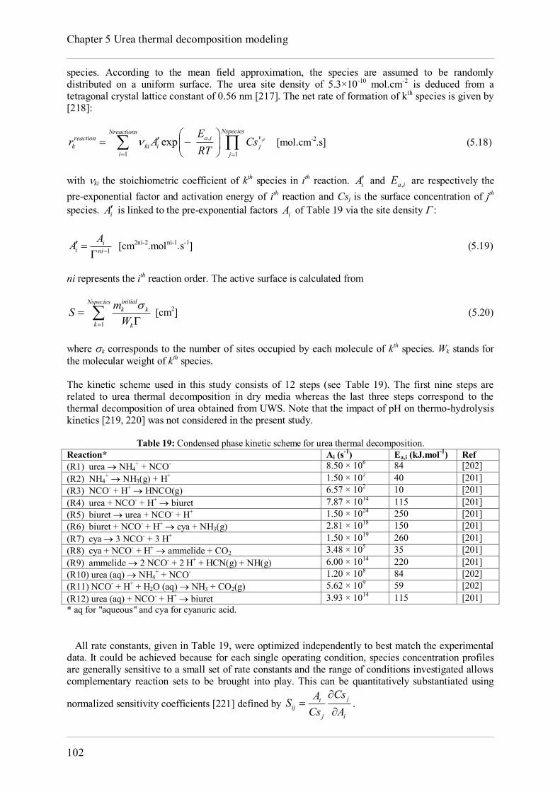
Chapter 5 Urea thermal decomposition modeling
102
species. According to the mean field approximation, the species are assumed to be randomly distributed on a uniform surface. The urea site density of 5.3×10⁻¹⁰ mol.cm-2 is deduced from a tetragonal crystal lattice constant of 0.56 nm [217]. The net rate of formation of kth species is given by [218]:
,
1 1
exp jiNspeciesNreactions
va ireactionk ki i j
i j
Er A Cs
RT
[mol.cm-2.s] (5.18)
with ki the stoichiometric coefficient of kth species in ith reaction. iA and ,a iE are respectively the pre-exponential factor and activation energy of ith reaction and Csj is the surface concentration of jth species. iA is linked to the pre-exponential factors iA of Table 19 via the site density
1i
i ni
AA
[cm2ni-2.molni-1.s-1] (5.19)
ni represents the ith reaction order. The active surface is calculated from
1
initialNspeciesk k
k k
mSW
[cm2] (5.20)
where k corresponds to the number of sites occupied by each molecule of kth species. Wk stands for the molecular weight of kth species. The kinetic scheme used in this study consists of 12 steps (see Table 19). The first nine steps are related to urea thermal decomposition in dry media whereas the last three steps correspond to the thermal decomposition of urea obtained from UWS. Note that the impact of pH on thermo-hydrolysis kinetics [219, 220] was not considered in the present study.
Table 19: Condensed phase kinetic scheme for urea thermal decomposition. Reaction* Ai (s-1) Ea,i (kJ.mol-1) Ref (R1) urea NH4
+ + NCO- 8.50 × 10⁶ 84 [202] (R2) NH4
+ NH3(g) + H+ 1.50 × 10² 40 [201] (R3) NCO- + H+ HNCO(g) 6.57 × 10² 10 [201] (R4) urea + NCO- + H+ biuret 7.87 × 10¹⁴ 115 [201] (R5) biuret urea + NCO- + H+ 1.50 × 1024 250 [201] (R6) biuret + NCO- + H+ cya + NH3(g) 2.81 × 10¹⁸ 150 [201] (R7) cya 3 NCO- + 3 H+ 1.50 × 10¹⁹ 260 [201] (R8) cya + NCO- + H+ ammelide + CO2 3.48 × 10⁵ 35 [201] (R9) ammelide 2 NCO- + 2 H+ + HCN(g) + NH(g) 6.00 × 10¹⁴ 220 [201] (R10) urea (aq) NH4
+ + NCO- 1.20 × 10⁸ 84 [202] (R11) NCO- + H+ + H2O (aq) NH3 + CO2(g) 5.62 × 10⁹ 59 [202] (R12) urea (aq) + NCO- + H+ biuret 3.93 × 10¹⁴ 115 [201] * aq for "aqueous" and cya for cyanuric acid. All rate constants, given in Table 19, were optimized independently to best match the experimental data. It could be achieved because for each single operating condition, species concentration profiles are generally sensitive to a small set of rate constants and the range of conditions investigated allows complementary reaction sets to be brought into play. This can be quantitatively substantiated using
normalized sensitivity coefficients [221] defined by jiij
j i
CsASCs A
.
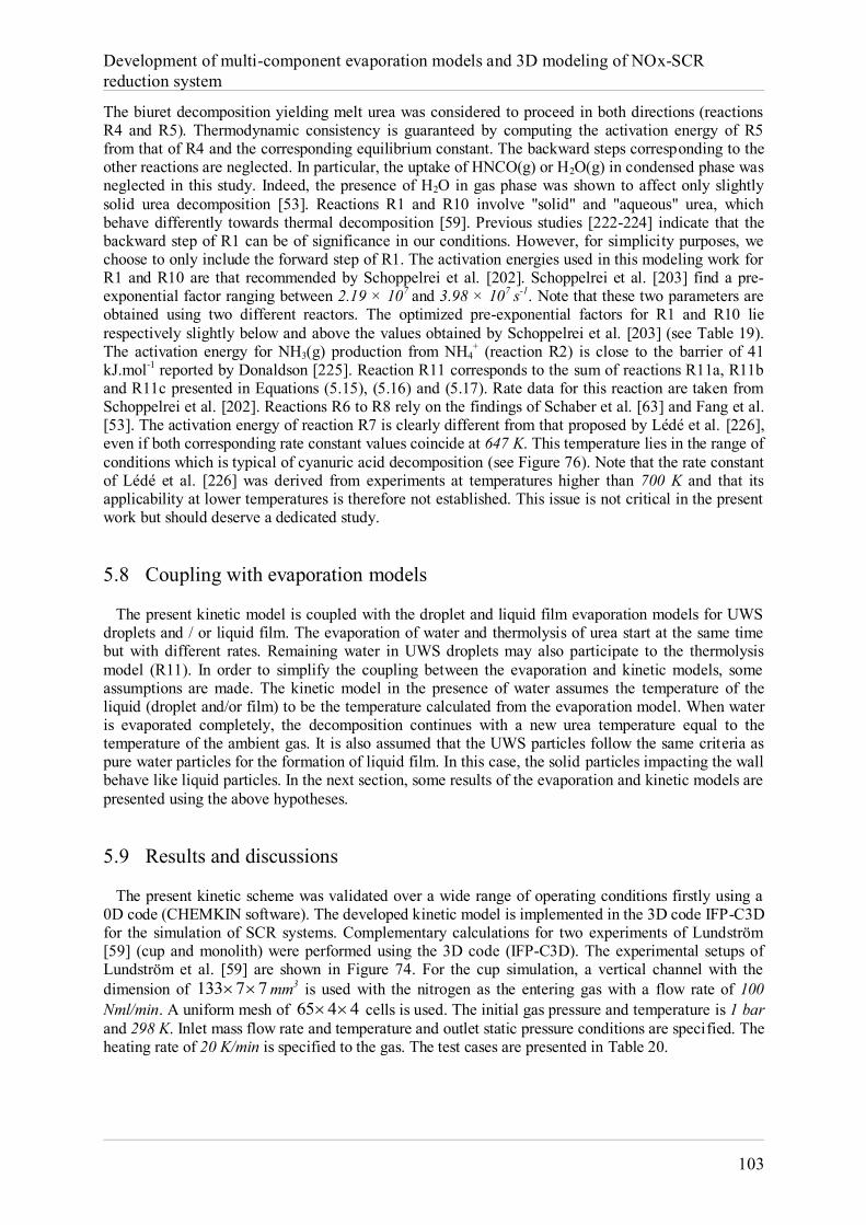
Development of multi-component evaporation models and 3D modeling of NOx-SCR reduction system
103
The biuret decomposition yielding melt urea was considered to proceed in both directions (reactions R4 and R5). Thermodynamic consistency is guaranteed by computing the activation energy of R5 from that of R4 and the corresponding equilibrium constant. The backward steps corresponding to the other reactions are neglected. In particular, the uptake of HNCO(g) or H2O(g) in condensed phase was neglected in this study. Indeed, the presence of H2O in gas phase was shown to affect only slightly solid urea decomposition [53]. Reactions R1 and R10 involve "solid" and "aqueous" urea, which behave differently towards thermal decomposition [59]. Previous studies [222-224] indicate that the backward step of R1 can be of significance in our conditions. However, for simplicity purposes, we choose to only include the forward step of R1. The activation energies used in this modeling work for R1 and R10 are that recommended by Schoppelrei et al. [202]. Schoppelrei et al. [203] find a pre-exponential factor ranging between 2.19 × 10⁷ and 3.98 × 10⁷ s-1. Note that these two parameters are obtained using two different reactors. The optimized pre-exponential factors for R1 and R10 lie respectively slightly below and above the values obtained by Schoppelrei et al. [203] (see Table 19). The activation energy for NH3(g) production from NH4
+ (reaction R2) is close to the barrier of 41 kJ.mol-1 reported by Donaldson [225]. Reaction R11 corresponds to the sum of reactions R11a, R11b and R11c presented in Equations (5.15), (5.16) and (5.17). Rate data for this reaction are taken from Schoppelrei et al. [202]. Reactions R6 to R8 rely on the findings of Schaber et al. [63] and Fang et al. [53]. The activation energy of reaction R7 is clearly different from that proposed by Lédé et al. [226], even if both corresponding rate constant values coincide at 647 K. This temperature lies in the range of conditions which is typical of cyanuric acid decomposition (see Figure 76). Note that the rate constant of Lédé et al. [226] was derived from experiments at temperatures higher than 700 K and that its applicability at lower temperatures is therefore not established. This issue is not critical in the present work but should deserve a dedicated study. 5.8 Coupling with evaporation models The present kinetic model is coupled with the droplet and liquid film evaporation models for UWS droplets and / or liquid film. The evaporation of water and thermolysis of urea start at the same time but with different rates. Remaining water in UWS droplets may also participate to the thermolysis model (R11). In order to simplify the coupling between the evaporation and kinetic models, some assumptions are made. The kinetic model in the presence of water assumes the temperature of the liquid (droplet and/or film) to be the temperature calculated from the evaporation model. When water is evaporated completely, the decomposition continues with a new urea temperature equal to the temperature of the ambient gas. It is also assumed that the UWS particles follow the same criteria as pure water particles for the formation of liquid film. In this case, the solid particles impacting the wall behave like liquid particles. In the next section, some results of the evaporation and kinetic models are presented using the above hypotheses. 5.9 Results and discussions The present kinetic scheme was validated over a wide range of operating conditions firstly using a 0D code (CHEMKIN software). The developed kinetic model is implemented in the 3D code IFP-C3D for the simulation of SCR systems. Complementary calculations for two experiments of Lundström [59] (cup and monolith) were performed using the 3D code (IFP-C3D). The experimental setups of Lundström et al. [59] are shown in Figure 74. For the cup simulation, a vertical channel with the dimension of 133 7 7 mm3 is used with the nitrogen as the entering gas with a flow rate of 100 Nml/min. A uniform mesh of 65 4 4 cells is used. The initial gas pressure and temperature is 1 bar and 298 K. Inlet mass flow rate and temperature and outlet static pressure conditions are specified. The heating rate of 20 K/min is specified to the gas. The test cases are presented in Table 20.
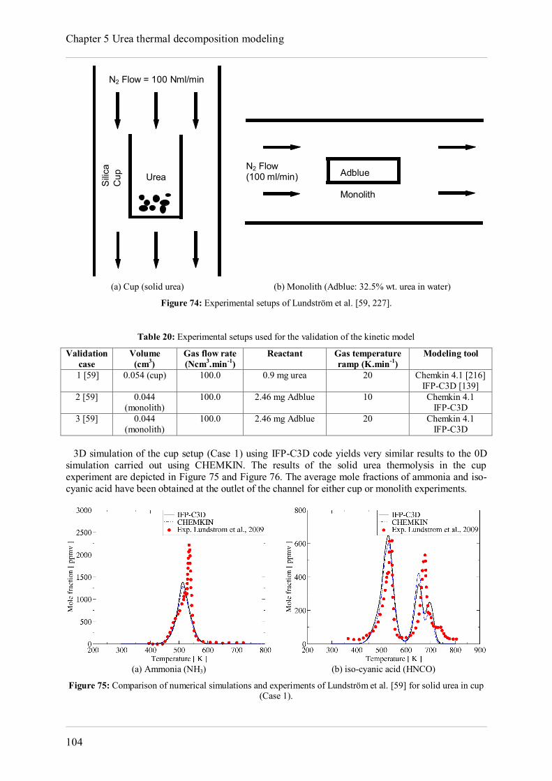
Chapter 5 Urea thermal decomposition modeling
104
(a) Cup (solid urea) (b) Monolith (Adblue: 32.5% wt. urea in water)
Figure 74: Experimental setups of Lundström et al. [59, 227].
Table 20: Experimental setups used for the validation of the kinetic model
Validation case
Volume (cm3)
Gas flow rate (Ncm3.min-1)
Reactant Gas temperature ramp (K.min-1)
Modeling tool
1 [59] 0.054 (cup) 100.0 0.9 mg urea 20 Chemkin 4.1 [216] IFP-C3D [139]
2 [59] 0.044 (monolith)
100.0 2.46 mg Adblue 10 Chemkin 4.1 IFP-C3D
3 [59] 0.044 (monolith)
100.0 2.46 mg Adblue 20 Chemkin 4.1 IFP-C3D
3D simulation of the cup setup (Case 1) using IFP-C3D code yields very similar results to the 0D simulation carried out using CHEMKIN. The results of the solid urea thermolysis in the cup experiment are depicted in Figure 75 and Figure 76. The average mole fractions of ammonia and iso-cyanic acid have been obtained at the outlet of the channel for either cup or monolith experiments.
(a) Ammonia (NH3) (b) iso-cyanic acid (HNCO)
Figure 75: Comparison of numerical simulations and experiments of Lundström et al. [59] for solid urea in cup (Case 1).
N2 Flow = 100 Nml/min
Urea
Silic
a C
up N2 Flow
(100 ml/min) Adblue
Monolith
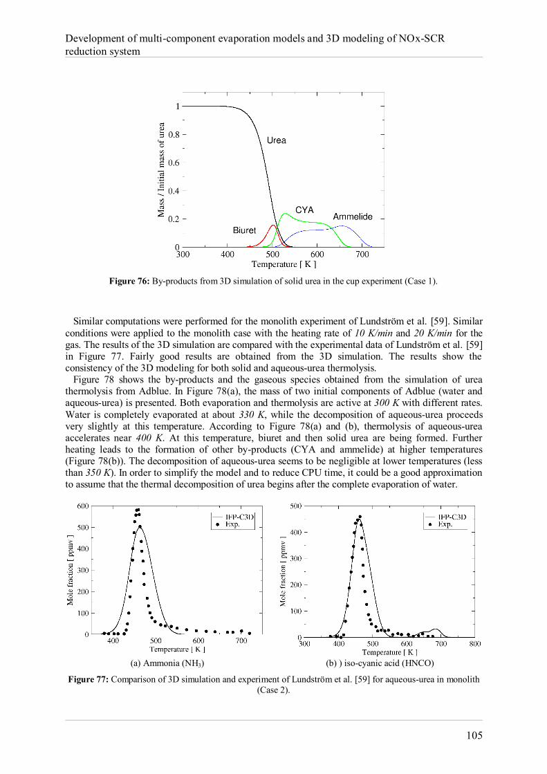
Development of multi-component evaporation models and 3D modeling of NOx-SCR reduction system
105
Figure 76: By-products from 3D simulation of solid urea in the cup experiment (Case 1).
Similar computations were performed for the monolith experiment of Lundström et al. [59]. Similar conditions were applied to the monolith case with the heating rate of 10 K/min and 20 K/min for the gas. The results of the 3D simulation are compared with the experimental data of Lundström et al. [59] in Figure 77. Fairly good results are obtained from the 3D simulation. The results show the consistency of the 3D modeling for both solid and aqueous-urea thermolysis. Figure 78 shows the by-products and the gaseous species obtained from the simulation of urea thermolysis from Adblue. In Figure 78(a), the mass of two initial components of Adblue (water and aqueous-urea) is presented. Both evaporation and thermolysis are active at 300 K with different rates. Water is completely evaporated at about 330 K, while the decomposition of aqueous-urea proceeds very slightly at this temperature. According to Figure 78(a) and (b), thermolysis of aqueous-urea accelerates near 400 K. At this temperature, biuret and then solid urea are being formed. Further heating leads to the formation of other by-products (CYA and ammelide) at higher temperatures (Figure 78(b)). The decomposition of aqueous-urea seems to be negligible at lower temperatures (less than 350 K). In order to simplify the model and to reduce CPU time, it could be a good approximation to assume that the thermal decomposition of urea begins after the complete evaporation of water.
(a) Ammonia (NH3) (b) ) iso-cyanic acid (HNCO)
Figure 77: Comparison of 3D simulation and experiment of Lundström et al. [59] for aqueous-urea in monolith (Case 2).
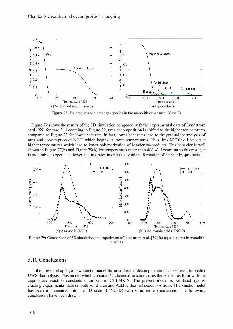
Chapter 5 Urea thermal decomposition modeling
106
(a) Water and aqueous-urea (b) By-products
Figure 78: By-products and other gas species in the monolith experiment (Case 2).
Figure 79 shows the results of the 3D simulation compared with the experimental data of Lundström et al. [59] for case 3. According to Figure 79, urea decomposition is shifted to the higher temperatures compared to Figure 77 for lower heat rate. In fact, lower heat rates lead to the gradual thermolysis of urea and consumption of NCO- which begins at lower temperatures. Thus, less NCO- will be left at higher temperatures which lead to lower polymerization of heavier by-products. This behavior is well shown in Figure 77(b) and Figure 79(b) for temperatures more than 600 K. According to this result, it is preferable to operate at lower heating rates in order to avoid the formation of heavier by-products.
(a) Ammonia (NH3) (b) ) iso-cyanic acid (HNCO)
Figure 79: Comparison of 3D simulation and experiment of Lundström et al. [59] for aqueous-urea in monolith (Case 3).
5.10 Conclusions In the present chapter, a new kinetic model for urea thermal decomposition has been used to predict UWS thermolysis. This model which contains 12 chemical reactions uses the Arrhenius form with the appropriate reaction constants optimized in CHEMKIN. The present model is validated against existing experimental data on both solid urea and Adblue thermal decompositions. The kinetic model has been implemented into the 3D code (IFP-C3D) with some more simulations. The following conclusions have been drawn:
Development of multi-component evaporation models and 3D modeling of NOx-SCR reduction system
107
The 0D and 3D simulations of solid urea and Adblue thermal decomposition show good
agreement between the model and the experiments. The new kinetic model represents well the behavior of species in each phase.
It is shown that the heating rate affects the thermolysis. Decreasing the heating rate (10 K/min instead of 20 K/min) causes the HNCO production to occur at lower temperatures.
It is found that urea decomposition is negligible during the evaporation process of water especially at low temperatures. Hence, the thermolysis of urea occurs mainly after the evaporation of water. This fact could help to simplify the modeling processes in SCR systems.
The hydrolysis (R11) is active during the evaporation of water. After the complete evaporation of water from Adblue, hydrolysis would not be active and it has no effect on the decomposition process. In the present study, it is assumed that after evaporation of water from Adblue, there is no residual water in the particle (no hydrates). Some amount of residual water in the particle may affect the thermolysis of urea and formation of HNCO. Further investigations on the existence and stability of residual water in the particles, at the end of evaporation and during the thermolysis, is needed.
More experimental data (typically experiments of Kim et al. [58]) could help to show more applicability of the new evaporation and kinetic models in realistic operating conditions.
In order to further improve the kinetic model, the two-way coupling of some reactions (like formation of NCO- from HNCO) could be considered. Also, the reactions leading to the polymerization should be further investigated.
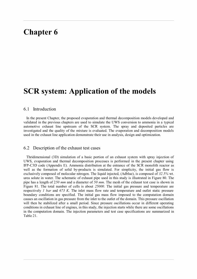
Chapter 6
SCR system: Application of the models 6.1 Introduction In the present Chapter, the proposed evaporation and thermal decomposition models developed and validated in the previous chapters are used to simulate the UWS conversion to ammonia in a typical automotive exhaust line upstream of the SCR system. The spray and deposited particles are investigated and the quality of the mixture is evaluated. The evaporation and decomposition models used in the exhaust line application demonstrate their use in analysis, design and optimization. 6.2 Description of the exhaust test cases Thridimensional (3D) simulation of a basic portion of an exhaust system with spray injection of UWS, evaporation and thermal decomposition processes is performed in the present chapter using IFP-C3D code (Appendix E). Ammonia distribution at the entrance of the SCR monolith reactor as well as the formation of solid by-products is simulated. For simplicity, the initial gas flow is exclusively composed of molecular nitrogen. The liquid injected, (Adblue), is composed of 32.5% wt. urea solute in water. The schematic of exhaust pipe used in this study is illustrated in Figure 80. The pipe has a length of 250 mm and a diameter of 50 mm. The mesh of the exhaust test case is shown in Figure 81. The total number of cells is about 25000. The initial gas pressure and temperature are respectively 1 bar and 673 K. The inlet mass flow rate and temperature and outlet static pressure boundary conditions are specified. The initial gas mass flow imposed to the computation domain causes an oscillation in gas pressure from the inlet to the outlet of the domain. This pressure oscillation will then be stabilized after a small period. Since pressure oscillations occur in different operating conditions in exhaust line of engines, in this study, the injection starts while there are some oscillations in the computation domain. The injection parameters and test case specifications are summarized in Table 21.
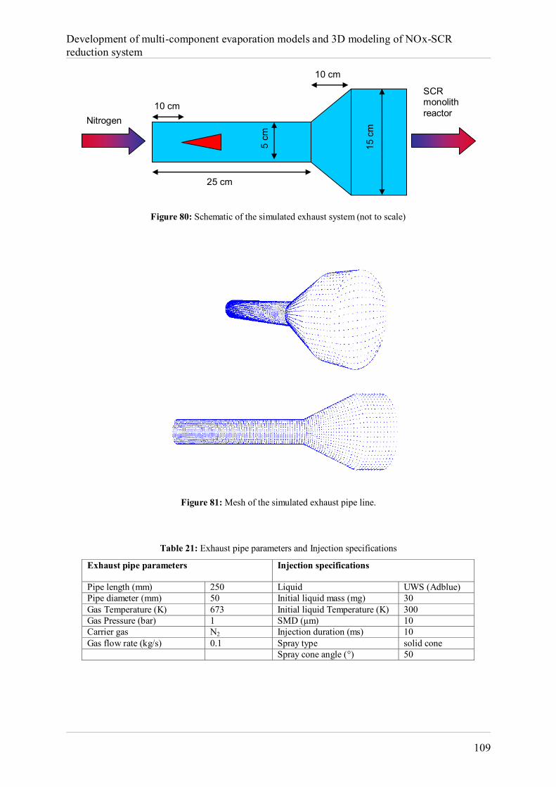
Development of multi-component evaporation models and 3D modeling of NOx-SCR reduction system
109
Figure 80: Schematic of the simulated exhaust system (not to scale)
Figure 81: Mesh of the simulated exhaust pipe line.
Table 21: Exhaust pipe parameters and Injection specifications
Exhaust pipe parameters
Injection specifications
Pipe length (mm) 250 Liquid UWS (Adblue) Pipe diameter (mm) 50 Initial liquid mass (mg) 30 Gas Temperature (K) 673 Initial liquid Temperature (K) 300 Gas Pressure (bar) 1 SMD (µm) 10 Carrier gas N2 Injection duration (ms) 10 Gas flow rate (kg/s) 0.1 Spray type solid cone Spray cone angle (°) 50
25 cm
10 cm
10 cm
5 cm
15 c
m Nitrogen
SCR monolith reactor
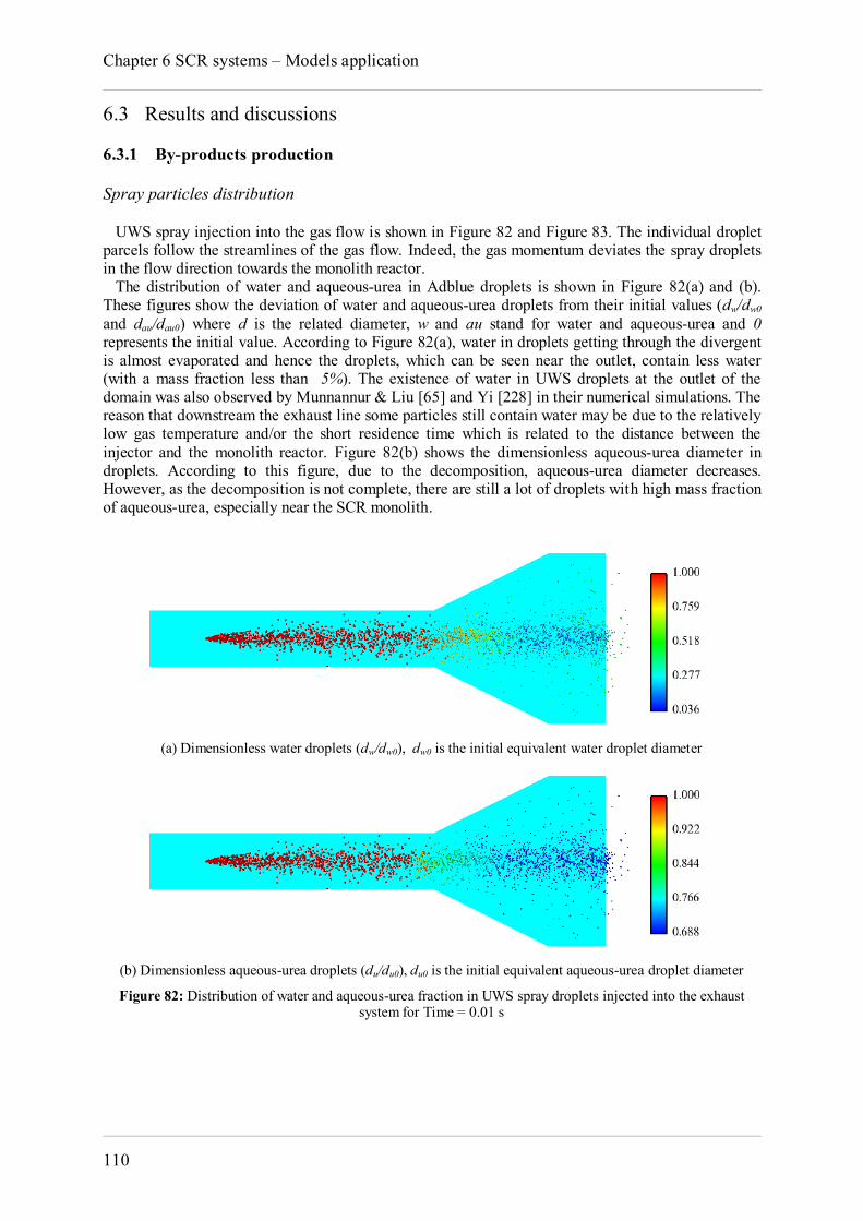
Chapter 6 SCR systems – Models application
110
6.3 Results and discussions 6.3.1 By-products production Spray particles distribution UWS spray injection into the gas flow is shown in Figure 82 and Figure 83. The individual droplet parcels follow the streamlines of the gas flow. Indeed, the gas momentum deviates the spray droplets in the flow direction towards the monolith reactor. The distribution of water and aqueous-urea in Adblue droplets is shown in Figure 82(a) and (b). These figures show the deviation of water and aqueous-urea droplets from their initial values (dw/dw0 and dau/dau0) where d is the related diameter, w and au stand for water and aqueous-urea and 0 represents the initial value. According to Figure 82(a), water in droplets getting through the divergent is almost evaporated and hence the droplets, which can be seen near the outlet, contain less water (with a mass fraction less than 5%). The existence of water in UWS droplets at the outlet of the domain was also observed by Munnannur & Liu [65] and Yi [228] in their numerical simulations. The reason that downstream the exhaust line some particles still contain water may be due to the relatively low gas temperature and/or the short residence time which is related to the distance between the injector and the monolith reactor. Figure 82(b) shows the dimensionless aqueous-urea diameter in droplets. According to this figure, due to the decomposition, aqueous-urea diameter decreases. However, as the decomposition is not complete, there are still a lot of droplets with high mass fraction of aqueous-urea, especially near the SCR monolith.
(a) Dimensionless water droplets (dw/dw0), dw0 is the initial equivalent water droplet diameter
(b) Dimensionless aqueous-urea droplets (du/du0), du0 is the initial equivalent aqueous-urea droplet diameter
Figure 82: Distribution of water and aqueous-urea fraction in UWS spray droplets injected into the exhaust system for Time = 0.01 s
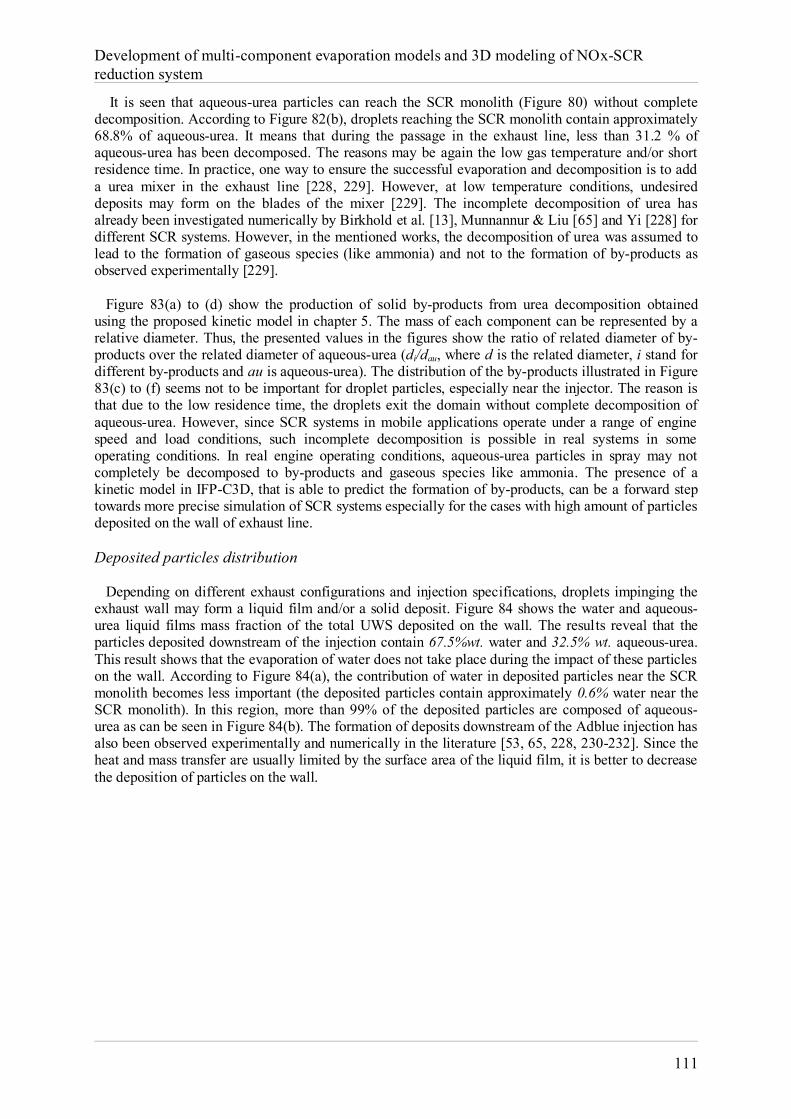
Development of multi-component evaporation models and 3D modeling of NOx-SCR reduction system
111
It is seen that aqueous-urea particles can reach the SCR monolith (Figure 80) without complete decomposition. According to Figure 82(b), droplets reaching the SCR monolith contain approximately 68.8% of aqueous-urea. It means that during the passage in the exhaust line, less than 31.2 % of aqueous-urea has been decomposed. The reasons may be again the low gas temperature and/or short residence time. In practice, one way to ensure the successful evaporation and decomposition is to add a urea mixer in the exhaust line [228, 229]. However, at low temperature conditions, undesired deposits may form on the blades of the mixer [229]. The incomplete decomposition of urea has already been investigated numerically by Birkhold et al. [13], Munnannur & Liu [65] and Yi [228] for different SCR systems. However, in the mentioned works, the decomposition of urea was assumed to lead to the formation of gaseous species (like ammonia) and not to the formation of by-products as observed experimentally [229]. Figure 83(a) to (d) show the production of solid by-products from urea decomposition obtained using the proposed kinetic model in chapter 5. The mass of each component can be represented by a relative diameter. Thus, the presented values in the figures show the ratio of related diameter of by-products over the related diameter of aqueous-urea (di/dau, where d is the related diameter, i stand for different by-products and au is aqueous-urea). The distribution of the by-products illustrated in Figure 83(c) to (f) seems not to be important for droplet particles, especially near the injector. The reason is that due to the low residence time, the droplets exit the domain without complete decomposition of aqueous-urea. However, since SCR systems in mobile applications operate under a range of engine speed and load conditions, such incomplete decomposition is possible in real systems in some operating conditions. In real engine operating conditions, aqueous-urea particles in spray may not completely be decomposed to by-products and gaseous species like ammonia. The presence of a kinetic model in IFP-C3D, that is able to predict the formation of by-products, can be a forward step towards more precise simulation of SCR systems especially for the cases with high amount of particles deposited on the wall of exhaust line. Deposited particles distribution Depending on different exhaust configurations and injection specifications, droplets impinging the exhaust wall may form a liquid film and/or a solid deposit. Figure 84 shows the water and aqueous-urea liquid films mass fraction of the total UWS deposited on the wall. The results reveal that the particles deposited downstream of the injection contain 67.5%wt. water and 32.5% wt. aqueous-urea. This result shows that the evaporation of water does not take place during the impact of these particles on the wall. According to Figure 84(a), the contribution of water in deposited particles near the SCR monolith becomes less important (the deposited particles contain approximately 0.6% water near the SCR monolith). In this region, more than 99% of the deposited particles are composed of aqueous-urea as can be seen in Figure 84(b). The formation of deposits downstream of the Adblue injection has also been observed experimentally and numerically in the literature [53, 65, 228, 230-232]. Since the heat and mass transfer are usually limited by the surface area of the liquid film, it is better to decrease the deposition of particles on the wall.
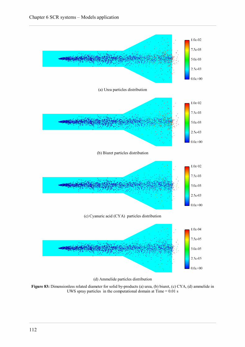
Chapter 6 SCR systems – Models application
112
(a) Urea particles distribution
(b) Biuret particles distribution
(c) Cyanuric acid (CYA) particles distribution
(d) Ammelide particles distribution
Figure 83: Dimensionless related diameter for solid by-products (a) urea, (b) biuret, (c) CYA, (d) ammelide in UWS spray particles in the computational domain at Time = 0.01 s
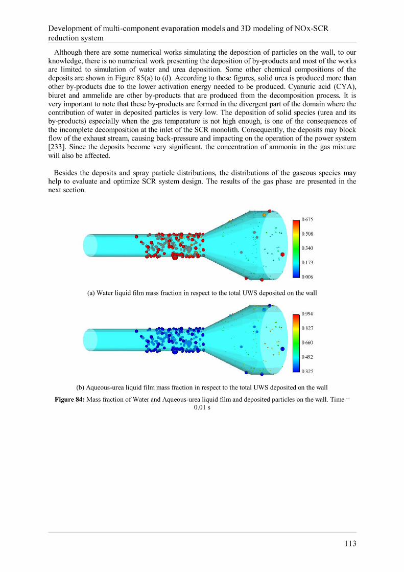
Development of multi-component evaporation models and 3D modeling of NOx-SCR reduction system
113
Although there are some numerical works simulating the deposition of particles on the wall, to our knowledge, there is no numerical work presenting the deposition of by-products and most of the works are limited to simulation of water and urea deposition. Some other chemical compositions of the deposits are shown in Figure 85(a) to (d). According to these figures, solid urea is produced more than other by-products due to the lower activation energy needed to be produced. Cyanuric acid (CYA), biuret and ammelide are other by-products that are produced from the decomposition process. It is very important to note that these by-products are formed in the divergent part of the domain where the contribution of water in deposited particles is very low. The deposition of solid species (urea and its by-products) especially when the gas temperature is not high enough, is one of the consequences of the incomplete decomposition at the inlet of the SCR monolith. Consequently, the deposits may block flow of the exhaust stream, causing back-pressure and impacting on the operation of the power system [233]. Since the deposits become very significant, the concentration of ammonia in the gas mixture will also be affected. Besides the deposits and spray particle distributions, the distributions of the gaseous species may help to evaluate and optimize SCR system design. The results of the gas phase are presented in the next section.
(a) Water liquid film mass fraction in respect to the total UWS deposited on the wall
(b) Aqueous-urea liquid film mass fraction in respect to the total UWS deposited on the wall
Figure 84: Mass fraction of Water and Aqueous-urea liquid film and deposited particles on the wall. Time = 0.01 s
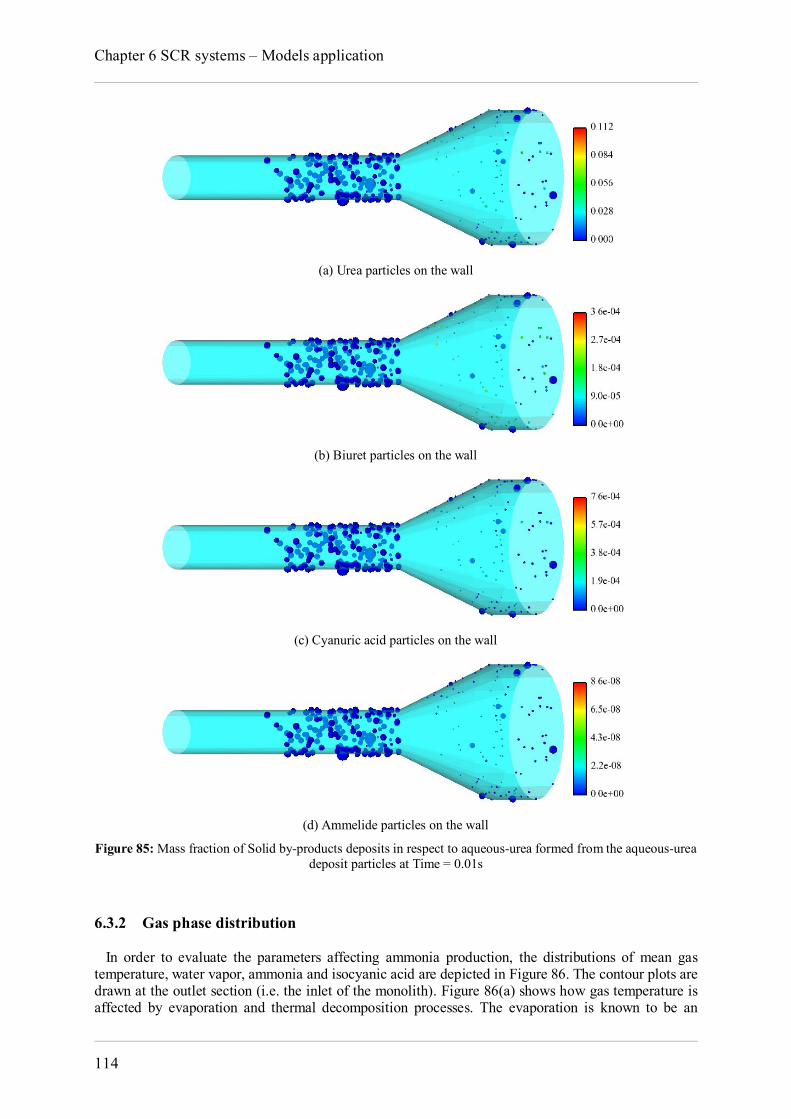
Chapter 6 SCR systems – Models application
114
(a) Urea particles on the wall
(b) Biuret particles on the wall
(c) Cyanuric acid particles on the wall
(d) Ammelide particles on the wall
Figure 85: Mass fraction of Solid by-products deposits in respect to aqueous-urea formed from the aqueous-urea deposit particles at Time = 0.01s
6.3.2 Gas phase distribution In order to evaluate the parameters affecting ammonia production, the distributions of mean gas temperature, water vapor, ammonia and isocyanic acid are depicted in Figure 86. The contour plots are drawn at the outlet section (i.e. the inlet of the monolith). Figure 86(a) shows how gas temperature is affected by evaporation and thermal decomposition processes. The evaporation is known to be an
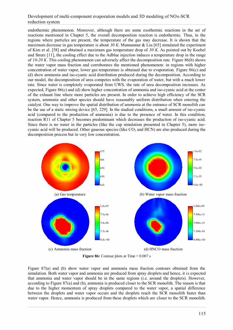
Development of multi-component evaporation models and 3D modeling of NOx-SCR reduction system
115
endothermic phenomenon. Moreover, although there are some exothermic reactions in the set of reactions mentioned in Chapter 5, the overall decomposition reaction is endothermic. Thus, in the regions where particles are present, the temperature of the gas may decrease. It is shown that the maximum decrease in gas temperature is about 30 K. Munnannur & Liu [65] simulated the experiment of Kim et al. [58] and obtained a maximum gas temperature drop of 30 K. As pointed out by Koebel and Strutz [11], the cooling effect due to the Adblue injection induces a temperature drop in the range of 10-20 K. This cooling phenomenon can adversely affect the decomposition rate. Figure 86(b) shows the water vapor mass fraction and corroborates the mentioned phenomenon: in regions with higher concentration of water vapor, lower gas temperature is obtained due to evaporation. Figure 86(c) and (d) show ammonia and iso-cyanic acid distribution produced during the decomposition. According to our model, the decomposition of urea competes with the evaporation of water, but with a much lower rate. Since water is completely evaporated from UWS, the rate of urea decomposition increases. As expected, Figure 86(c) and (d) show higher concentration of ammonia and iso-cyanic acid at the center of the exhaust line where more particles are present. In order to achieve high efficiency of the SCR system, ammonia and other species should have reasonably uniform distribution when entering the catalyst. One way to improve the spatial distribution of ammonia at the entrance of SCR monolith can be the use of a static mixing device [65, 229]. In the studied conditions, a small amount of iso-cyanic acid (compared to the production of ammonia) is due to the presence of water. In this condition, reaction R11 of Chapter 5 becomes predominant which decreases the production of iso-cyanic acid. Since there is no water in the particles (like the cup simulation presented in Chapter 5), more iso-cyanic acid will be produced. Other gaseous species (like CO2 and HCN) are also produced during the decomposition process but in very low concentration.
(a) Gas temperature (b) Water vapor mass fraction
(c) Ammonia mass fraction (d) HNCO mass fraction
Figure 86: Contour plots at Time = 0.007 s
Figure 87(a) and (b) show water vapor and ammonia mass fraction contours obtained from the simulation. Both water vapor and ammonia are produced from spray droplets and hence, it is expected that ammonia and water vapor should be in the same regions (i.e. around the droplets). However, according to Figure 87(a) and (b), ammonia is produced closer to the SCR monolith. The reason is that due to the higher momentum of spray droplets compared to the water vapor, a spatial difference between the droplets and water vapor occurs and the droplets reach the SCR monolith faster than water vapor. Hence, ammonia is produced from these droplets which are closer to the SCR monolith.
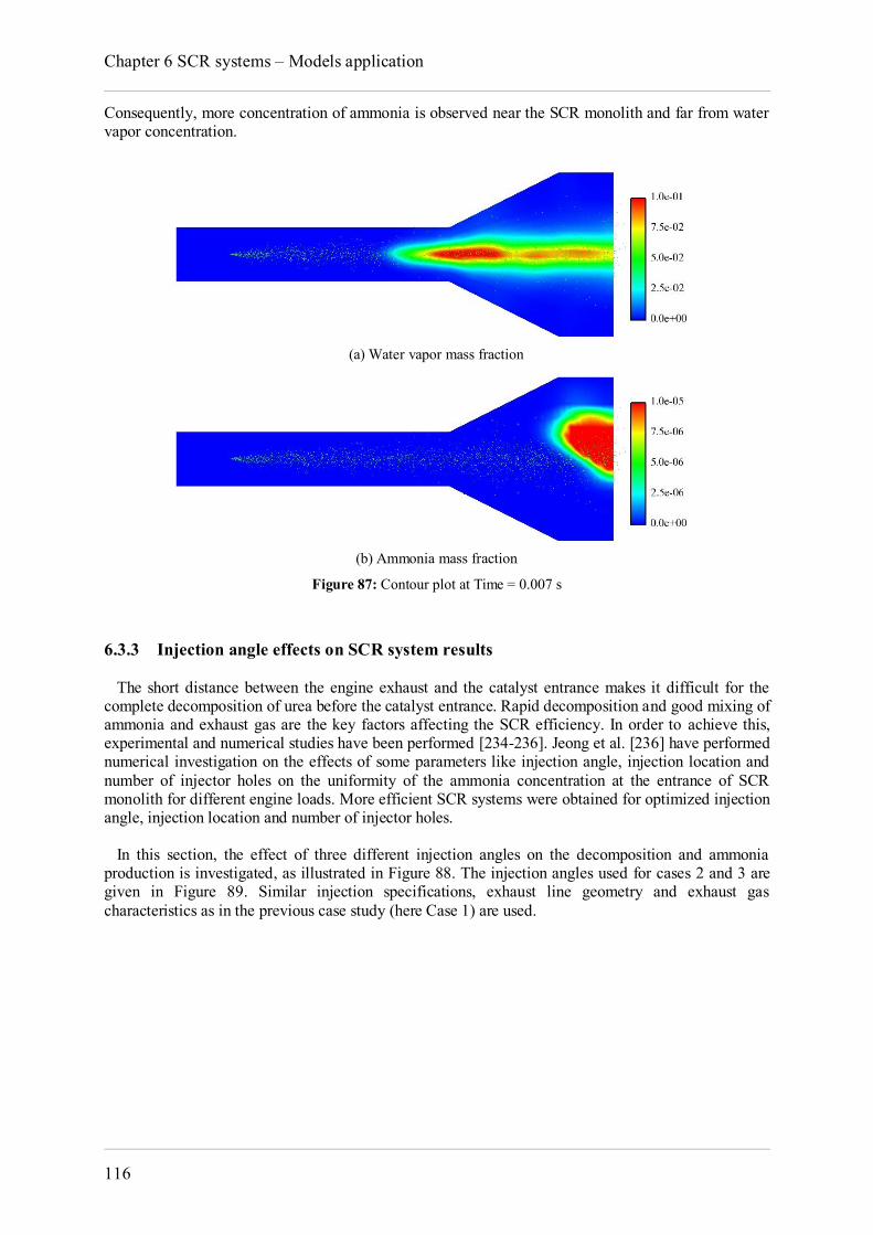
Chapter 6 SCR systems – Models application
116
Consequently, more concentration of ammonia is observed near the SCR monolith and far from water vapor concentration.
(a) Water vapor mass fraction
(b) Ammonia mass fraction
Figure 87: Contour plot at Time = 0.007 s
6.3.3 Injection angle effects on SCR system results The short distance between the engine exhaust and the catalyst entrance makes it difficult for the complete decomposition of urea before the catalyst entrance. Rapid decomposition and good mixing of ammonia and exhaust gas are the key factors affecting the SCR efficiency. In order to achieve this, experimental and numerical studies have been performed [234-236]. Jeong et al. [236] have performed numerical investigation on the effects of some parameters like injection angle, injection location and number of injector holes on the uniformity of the ammonia concentration at the entrance of SCR monolith for different engine loads. More efficient SCR systems were obtained for optimized injection angle, injection location and number of injector holes. In this section, the effect of three different injection angles on the decomposition and ammonia production is investigated, as illustrated in Figure 88. The injection angles used for cases 2 and 3 are given in Figure 89. Similar injection specifications, exhaust line geometry and exhaust gas characteristics as in the previous case study (here Case 1) are used.
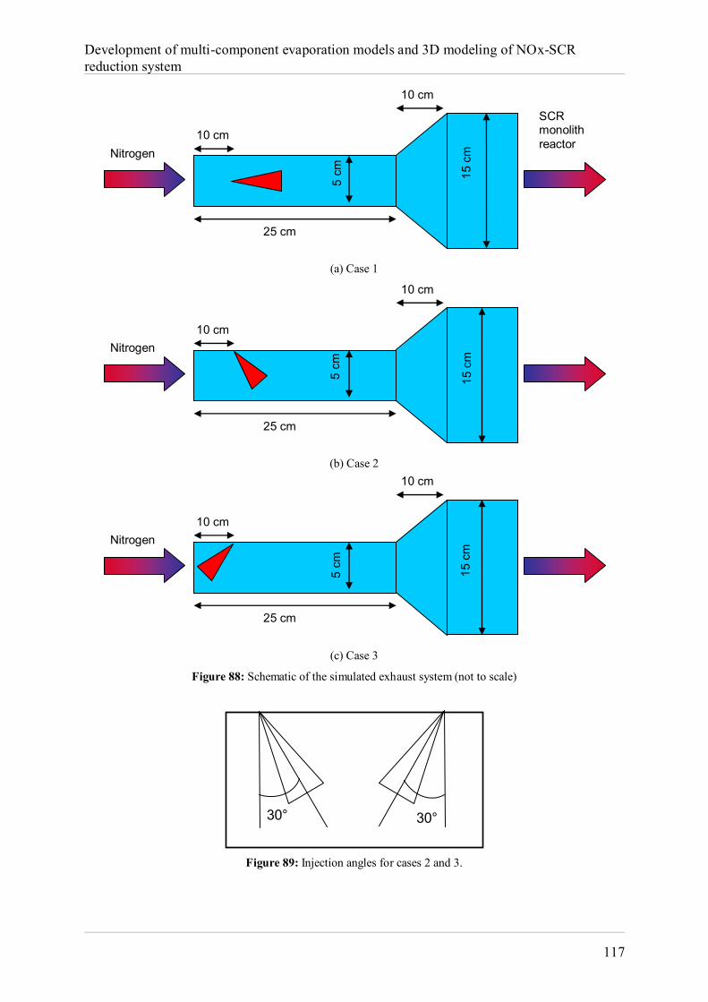
Development of multi-component evaporation models and 3D modeling of NOx-SCR reduction system
117
(a) Case 1
(b) Case 2
(c) Case 3
Figure 88: Schematic of the simulated exhaust system (not to scale)
Figure 89: Injection angles for cases 2 and 3.
25 cm
10 cm
10 cm
5 cm
15 c
m Nitrogen
25 cm
10 cm
10 cm 5
cm
15 c
m Nitrogen
25 cm
10 cm
10 cm
5 cm
15 c
m
Nitrogen
SCR monolith reactor
30° 30°
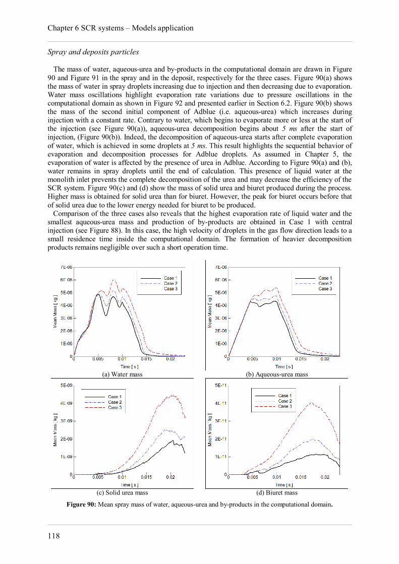
Chapter 6 SCR systems – Models application
118
Spray and deposits particles The mass of water, aqueous-urea and by-products in the computational domain are drawn in Figure 90 and Figure 91 in the spray and in the deposit, respectively for the three cases. Figure 90(a) shows the mass of water in spray droplets increasing due to injection and then decreasing due to evaporation. Water mass oscillations highlight evaporation rate variations due to pressure oscillations in the computational domain as shown in Figure 92 and presented earlier in Section 6.2. Figure 90(b) shows the mass of the second initial component of Adblue (i.e. aqueous-urea) which increases during injection with a constant rate. Contrary to water, which begins to evaporate more or less at the start of the injection (see Figure 90(a)), aqueous-urea decomposition begins about 5 ms after the start of injection, (Figure 90(b)). Indeed, the decomposition of aqueous-urea starts after complete evaporation of water, which is achieved in some droplets at 5 ms. This result highlights the sequential behavior of evaporation and decomposition processes for Adblue droplets. As assumed in Chapter 5, the evaporation of water is affected by the presence of urea in Adblue. According to Figure 90(a) and (b), water remains in spray droplets until the end of calculation. This presence of liquid water at the monolith inlet prevents the complete decomposition of the urea and may decrease the efficiency of the SCR system. Figure 90(c) and (d) show the mass of solid urea and biuret produced during the process. Higher mass is obtained for solid urea than for biuret. However, the peak for biuret occurs before that of solid urea due to the lower energy needed for biuret to be produced. Comparison of the three cases also reveals that the highest evaporation rate of liquid water and the smallest aqueous-urea mass and production of by-products are obtained in Case 1 with central injection (see Figure 88). In this case, the high velocity of droplets in the gas flow direction leads to a small residence time inside the computational domain. The formation of heavier decomposition products remains negligible over such a short operation time.
(a) Water mass (b) Aqueous-urea mass
(c) Solid urea mass (d) Biuret mass
Figure 90: Mean spray mass of water, aqueous-urea and by-products in the computational domain.
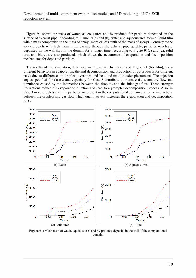
Development of multi-component evaporation models and 3D modeling of NOx-SCR reduction system
119
Figure 91 shows the mass of water, aqueous-urea and by-products for particles deposited on the surface of exhaust pipe. According to Figure 91(a) and (b), water and aqueous-urea form a liquid film with a mass comparable to the mass of spray (more or less tenth of the mass of spray). Contrary to the spray droplets with high momentum passing through the exhaust pipe quickly, particles which are deposited on the wall stay in the domain for a longer time. According to Figure 91(c) and (d), solid urea and biuret are also produced, which shows the occurrence of evaporation and decomposition mechanisms for deposited particles. The results of the simulation, illustrated in Figure 90 (for spray) and Figure 91 (for film), show different behaviors in evaporation, thermal decomposition and production of by-products for different cases due to differences in droplets dynamics and heat and mass transfer phenomena. The injection angles specified for Case 2 and especially for Case 3 contribute to increase the secondary flow and turbulence caused by the interactions between the droplets and the inlet gas flow. These stronger interactions reduce the evaporation duration and lead to a prompter decomposition process. Also, in Case 3 more droplets and film particles are present in the computational domain due to the interactions between the droplets and gas flow which quantitatively increases the evaporation and decomposition rates.
(a) Water (b) Aqueous-urea
(c) Solid urea (d) Biuret
Figure 91: Mean mass of water, aqueous-urea and by-products deposits in the wall of the computational domain.

Chapter 6 SCR systems – Models application
120
Figure 92: Pressure oscillations in the computation domain (Case 1)
Gas phase behavior Figure 93 shows the mean mole fraction of ammonia at the outlet of the computational domain for the three different cases. Case 2 shows a higher ammonia concentration at the outlet in the given time range. Gas temperature effects and the presence of water in droplet are the most important phenomena contributing to ammonia production. The presence of water in droplets can increase the ammonia production trough reaction R11 of Chapter 5. As assumed in the proposed kinetic model, since water is present in UWS, the temperature of reactions is the temperature of liquid and not the temperature of gas. When water is completely evaporated, the liquid temperature used for the chemical reactions is switched to the gas temperature. With the mentioned hypothesis, the presence of water can limit the general rate of ammonia production due to the low liquid temperature applied to the model. The higher production of ammonia in Case 2 may be due to the fact that some droplets or film particles achieve faster the gas temperature because of higher spray-gas interactions.
Figure 93: Comparison of NH3 mole fraction at the outlet of computation domain for three cases
Mass flow rate The quality of the gas mixture can be represented by the mass flux distribution of gaseous species, defined as [228]:
. . .i iM V AY (6.1)
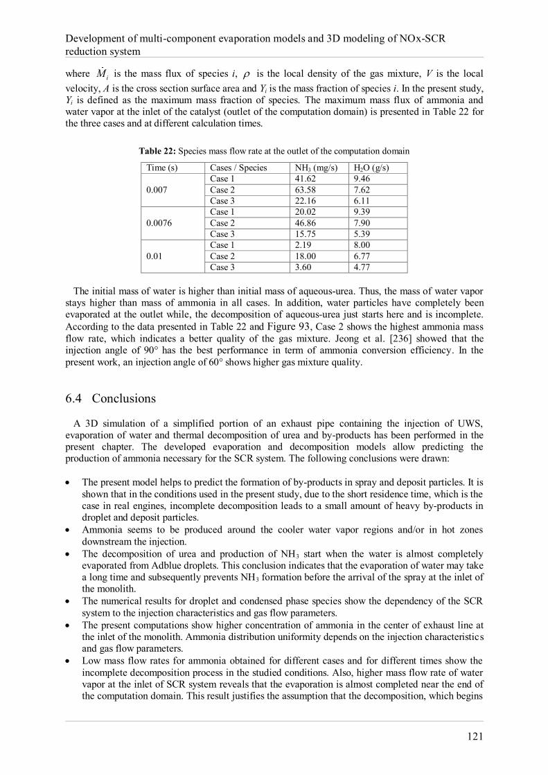
Development of multi-component evaporation models and 3D modeling of NOx-SCR reduction system
121
where iM is the mass flux of species i, is the local density of the gas mixture, V is the local velocity, A is the cross section surface area and Yi is the mass fraction of species i. In the present study, Yi is defined as the maximum mass fraction of species. The maximum mass flux of ammonia and water vapor at the inlet of the catalyst (outlet of the computation domain) is presented in Table 22 for the three cases and at different calculation times.
Table 22: Species mass flow rate at the outlet of the computation domain
Time (s) Cases / Species NH3 (mg/s) H2O (g/s)
0.007 Case 1 41.62 9.46 Case 2 63.58 7.62 Case 3 22.16 6.11
0.0076 Case 1 20.02 9.39 Case 2 46.86 7.90 Case 3 15.75 5.39
0.01 Case 1 2.19 8.00 Case 2 18.00 6.77 Case 3 3.60 4.77
The initial mass of water is higher than initial mass of aqueous-urea. Thus, the mass of water vapor stays higher than mass of ammonia in all cases. In addition, water particles have completely been evaporated at the outlet while, the decomposition of aqueous-urea just starts here and is incomplete. According to the data presented in Table 22 and Figure 93, Case 2 shows the highest ammonia mass flow rate, which indicates a better quality of the gas mixture. Jeong et al. [236] showed that the injection angle of 90° has the best performance in term of ammonia conversion efficiency. In the present work, an injection angle of 60° shows higher gas mixture quality. 6.4 Conclusions A 3D simulation of a simplified portion of an exhaust pipe containing the injection of UWS, evaporation of water and thermal decomposition of urea and by-products has been performed in the present chapter. The developed evaporation and decomposition models allow predicting the production of ammonia necessary for the SCR system. The following conclusions were drawn: The present model helps to predict the formation of by-products in spray and deposit particles. It is
shown that in the conditions used in the present study, due to the short residence time, which is the case in real engines, incomplete decomposition leads to a small amount of heavy by-products in droplet and deposit particles.
Ammonia seems to be produced around the cooler water vapor regions and/or in hot zones downstream the injection.
The decomposition of urea and production of NH3 start when the water is almost completely evaporated from Adblue droplets. This conclusion indicates that the evaporation of water may take a long time and subsequently prevents NH3 formation before the arrival of the spray at the inlet of the monolith.
The numerical results for droplet and condensed phase species show the dependency of the SCR system to the injection characteristics and gas flow parameters.
The present computations show higher concentration of ammonia in the center of exhaust line at the inlet of the monolith. Ammonia distribution uniformity depends on the injection characteristics and gas flow parameters.
Low mass flow rates for ammonia obtained for different cases and for different times show the incomplete decomposition process in the studied conditions. Also, higher mass flow rate of water vapor at the inlet of SCR system reveals that the evaporation is almost completed near the end of the computation domain. This result justifies the assumption that the decomposition, which begins
Chapter 6 SCR systems – Models application
122
after the complete evaporation of water, is incomplete and there is no enough time for the ammonia production process. Hence, the lower mass flow rate for ammonia is obtained.
More 3D simulations of exhaust system with different injector types and some comparisons with the experimental data would help to validate the developed models over a larger range of conditions.
Development of multi-component evaporation models and 3D modeling of NOx-SCR reduction system
123
Conclusions of Part II The present part of the thesis manuscript focused on the physical and chemical processes appearing from the injection of urea-water solution to the entrance of the SCR system. For this purpose, some related numerical models are developed. An evaporation model for water from UWS (droplet and film) is suggested which takes into account the influence of the solved urea on water evaporation using NRTL model. A kinetic model containing 12 reactions, which covers thermal decomposition of either solid or aqueous-urea, is developed. The kinetic and evaporation models have been validated with some experimental data. The following general conclusions were drawn from the second part of the thesis:
It is shown that the solved urea in UWS influences the physical behaviors of UWS. It increases the temperature of UWS by reducing the vapor pressure of the UWS. In addition, it decreases the evaporation of water due to the decrease in transport properties. However, it seems that urea has more influence on the temperature of UWS than the evaporation of water.
The numerical results of the evaporation and kinetic models are in good agreement with the experimental results.
0D and 3D simulations of the thermal decomposition of solid/aqueous urea point out the existence of by-products in different conditions.
The developed numerical models for evaporation and thermolysis allow the investigation of different processes in exhaust pipe line of internal engines. The proposed models help to evaluate the spatial distribution of ammonia as the reducing agent and other gaseous species. In addition, the kinetic model allows the prediction of the by-products depositions produced from the urea thermolysis and formed on the exhaust pipes for any exhaust configurations.
In order to increase the accuracy of the simulations, further investigations on the evaporation and thermolysis phenomena are necessary.
Chapter 7
Conclusions and Prospective 7.1 Summary of the thesis The thesis started by highlighting the importance of multi-component nature of fuels and its modeling effect on the mixture preparation and combustion in internal combustion engines. It was explained that a single-component model could not predict the contribution of the volatility of individual fuel components on the mixture preparation and combustion. Hence, a multi-component fuel evaporation model will improve the simulation results, and therefore will lead to less uncertainty in the prediction of the fuel vapor distribution especially in the zones with a large range of fuel volatilities. Two Lagrangian multi-component evaporation models for spray and liquid film have been developed in first part. Then, the advantages of the multi-component model have been demonstrated and the benefits of the developed models were illustrated by different simulation studies. In the second part, the study of NOx reduction in exhaust line of diesel engine led to the developing of new evaporation and kinetic models which help to predict the spatial distribution of reducing agent at the entrance of SCR system. The models applicability has been presented using different case studies. 7.2 Concluding remarks In the present section, the objectives of the work explained in different chapters are reviewed and the conclusions are presented. Chapter 1 provided the information regarding the development of a discrete multi-component droplet evaporation model with new features concerning the transport properties. This model uses a Stephan velocity to ensure gas mass conservation and takes into account the enthalpy diffusion of species in addition to the conduction heat flux. The influence of high pressure on the transport properties has been taken into account using real gas EOS. It has been shown that the new evaporation model improves the evaporation rate of liquid droplets. Chapter 2 was dedicated to the development of discrete multi-component liquid film evaporation. The conclusion that emerged from the model development is that the effect of wall temperature is more important than the effect of gas temperature on the film temperature and film evaporation. It was also shown that the real and ideal gas models have similar behavior in both droplet and liquid film models.
Development of multi-component evaporation models and 3D modeling of NOx-SCR reduction system
125
Chapter 3 presented some applications of the spray and liquid film evaporation models in diesel engine configurations using different fuel models. The numerical results of the evaporation models allow assessing the contribution of the developments made during this work in the context of industrial applications. Chapter 4 focused on the development of evaporation models for UWS droplets as well as liquid film. The evaporation models proposed in Chapter 1 and Chapter 2 were modified to take into account the effect of urea on the evaporation of water from UWS droplet and liquid film. It was concluded that the evaporation of water in the presence of urea is different from the evaporation of hydrocarbons and the influence of urea on the UWS temperature and evaporation rate should be considered in an appropriate evaporation model. Chapter 5 introduced a kinetic model for the thermal decomposition of urea from UWS. The presented kinetic model was then coupled with the modified evaporation model of Chapter 4 to investigate both physical and chemical behaviors of urea and UWS during the evaporation and thermal decomposition processes. Aside from the simplicity, it has been shown that the developed kinetic model is able to simulate the deposition of by-products formed during the thermolysis of urea. Chapter 6 simulated the distribution of ammonia and other gaseous species and also the formation of by-products in a typical exhaust system. It was concluded that the evaporation and kinetic models are very useful in real applications and can be used as a research tool for further investigations on the SCR DeNOx systems. 7.3 Recommendations for future work 7.3.1 Towards further improvement of droplet evaporation The proposed droplet evaporation model is based on some hypotheses which simplify the evaporation model. In the proposed evaporation model, infinite thermal conductivity model has been considered with the uniform temperature profile inside the droplet. Temperature profile and internal recirculation inside the droplet could increase the accuracy of the developed model by influencing on the transport properties. Further investigations on the effects of "effective thermal conduction model" [102] on the evaporation and transport phenomenon is needed. Furthermore, taking into account the diffusion of species in the liquid phase can further improve the evaporation model [107]. Developing a model which takes into account the transient effects in the gas phase especially for high pressure and temperature conditions is one of the challenges that future research should focus on. The present thesis assumed the droplets to be spheric. Further investigations on the non-spherical assumption of spray droplets especially for larger droplets are necessary. DNS Eulerian method could be used in the future in order to develop non-spherical droplets and ligaments evaporation. Droplet collisions modeling [237], the effect of droplet-droplet interaction in dense spray on the evaporation [238] and the influence of turbulence on droplet vaporization [239] and combustion [240] are other challenges that could be investigated using the new evaporation model. 7.3.2 Liquid film evaporation An investigation on the film-flame interaction phenomenon has been directed by Desoutter. Further investigations on the effects of multi-component fuel film on the film-flame interaction phenomenon in combustion chamber, especially for higher thickness of liquid film, is needed. Developing a laminar film evaporation model could be helpful in order to observe the behavior of liquid film in laminar zones. 7.3.3 Further investigations on the Equation of State Real gas hypothesis applied for both droplet and liquid film evaporation models for hydrocarbon fuels using PR-EOS. Further research should concentrate on developing evaporation models with
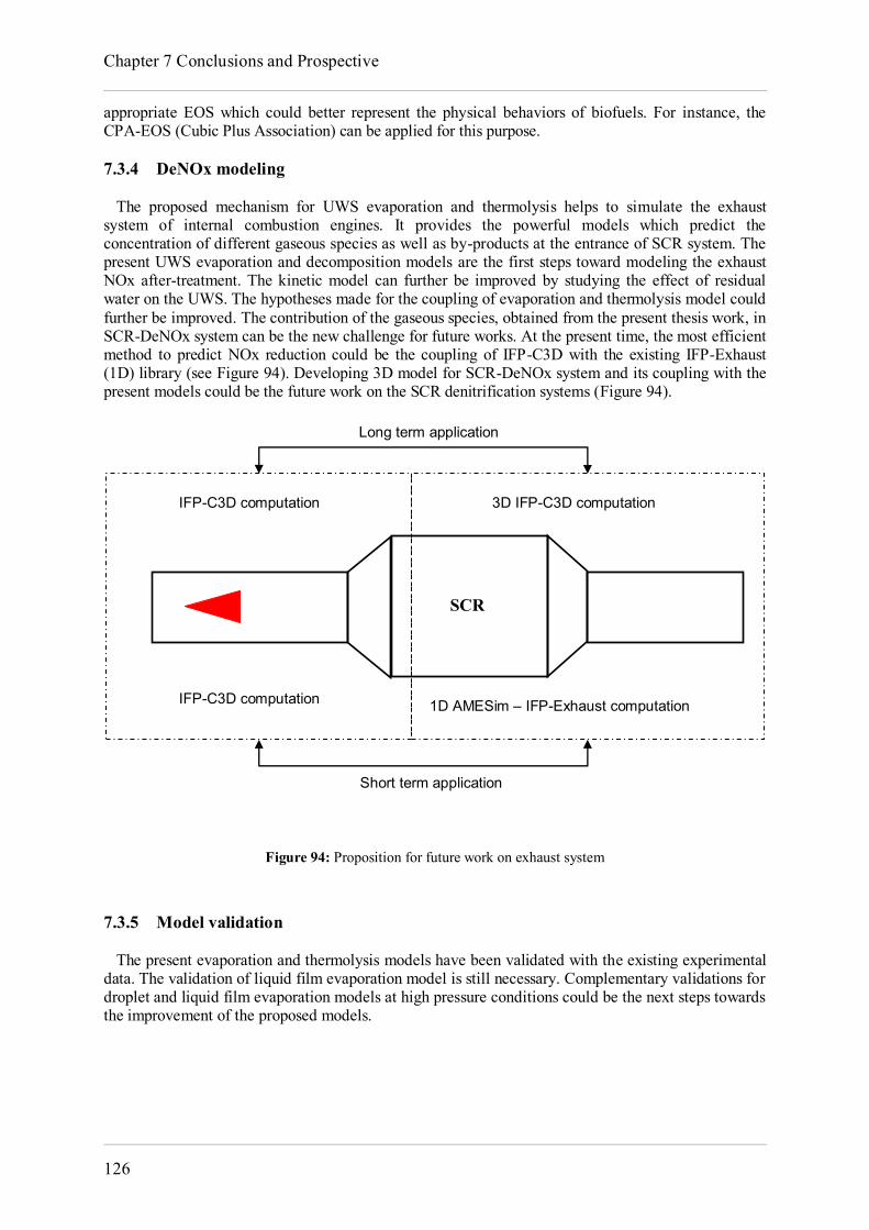
Chapter 7 Conclusions and Prospective
126
appropriate EOS which could better represent the physical behaviors of biofuels. For instance, the CPA-EOS (Cubic Plus Association) can be applied for this purpose. 7.3.4 DeNOx modeling The proposed mechanism for UWS evaporation and thermolysis helps to simulate the exhaust system of internal combustion engines. It provides the powerful models which predict the concentration of different gaseous species as well as by-products at the entrance of SCR system. The present UWS evaporation and decomposition models are the first steps toward modeling the exhaust NOx after-treatment. The kinetic model can further be improved by studying the effect of residual water on the UWS. The hypotheses made for the coupling of evaporation and thermolysis model could further be improved. The contribution of the gaseous species, obtained from the present thesis work, in SCR-DeNOx system can be the new challenge for future works. At the present time, the most efficient method to predict NOx reduction could be the coupling of IFP-C3D with the existing IFP-Exhaust (1D) library (see Figure 94). Developing 3D model for SCR-DeNOx system and its coupling with the present models could be the future work on the SCR denitrification systems (Figure 94).
Figure 94: Proposition for future work on exhaust system
7.3.5 Model validation The present evaporation and thermolysis models have been validated with the existing experimental data. The validation of liquid film evaporation model is still necessary. Complementary validations for droplet and liquid film evaporation models at high pressure conditions could be the next steps towards the improvement of the proposed models.
IFP-C3D computation
Short term application
Long term application
SCR
1D AMESim – IFP-Exhaust computation
3D IFP-C3D computation
IFP-C3D computation
Appendix A
Properties of the gas mixture
A.1. Properties used for droplet modeling Some properties like ρg, μg, Dg, hi and λg are calculated at the reference temperature Tref (Equation (1.30)) while others like ρ∞ and μ∞ are obtained at T∞. Density of the gas mixture is calculated from the ideal/real gas equation of state with the appropriate temperature. For the binary diffusion coefficient Dg in the gas mixture, the correlation of Wilke and Lee [130] has been used. Then, the diffusion coefficient of each species into the gas mixture is obtained from the following relation:
1 spec
spec spec
N
i iim N N
ii i
X WYD X XWD D
(8.1)
where Dai=Dg for component i. Dynamic viscosity and thermal conduction coefficients (λg (W.m-1K-1) and μg (Kg.m-1s-1)) are obtained at Tref:
3 2 51 1
2 2
252 10 with
200 ref
gref
AT AT A A K
(8.2)
3 2 9
1 1
2 2
1457 10 with
110 ref
gref
AT AT A A K
(8.3)
μ∞ is obtained from Equation (8.3) at the ambient temperature T∞. Specific heat of liquid at constant pressure Cpf is calculated from the enthalpy gradient at the reference temperature Tref. Specific enthalpy hi for each component is obtained from the tabulated thermodynamic data like Burcat [241].
A.1.1. Molar liquid volume For compressed liquids, the method of Hankinson-Brobst-Thomson (HBT) can be used. To estimate the molar volume of saturated liquids, method of HBT or Rackett can be used. In the method of HBT, the saturated liquid volume for the mixture is obtained by [242]:
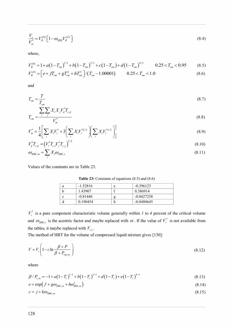
128
(0) ( )
* 1sR SRK R
m
V V VV
(8.4)
where,
1/3 2/3 4/3(0) 1 1 1 1 1 0.25 0.95R rm rm rm rm rmV a T b T c T d T T (8.5)
( ) 2 3 / 1.00001 0.25 1.0R rm rm rm rm rmV e fT gT hT T T (8.6) and
rmcm
TTT
(8.7)
*,
*
i j ij c iji j
cmm
X X V TT
V
(8.8)
* * *2/3 *1/31 34m i i i i i i
i i iV X V X V X V
(8.9)
1/ 2* * *
, , ,ij c ij i c i j c jV T V T V T (8.10)
, ,SRK m i SRK ii
X (8.11)
Values of the constants are in Table 23.
Table 23: Constants of equations (8.5) and (8.6)
a -1.52816 e -0.296123 b 1.43907 f 0.386914 c -0.81446 g -0.0427258 d 0.190454 h -0.0480645
*
iV is a pure component characteristic volume generally within 1 to 4 percent of the critical volume
and ,SRK i is the acentric factor and maybe replaced with . If the value of *iV is not available from
the tables, it maybe replaced with ,c iV . The method of HBT for the volume of compressed liquid mixture gives [130]:
,
1 lnsvap m
PV V cP
(8.12)
where
1/ 3 2 / 3 4 / 3
,/ 1 1 1 1 1c m r r r rP a T b T d T e T (8.13)
2, ,exp SRK m SRK me f g h (8.14)
,SRK mc j k (8.15)
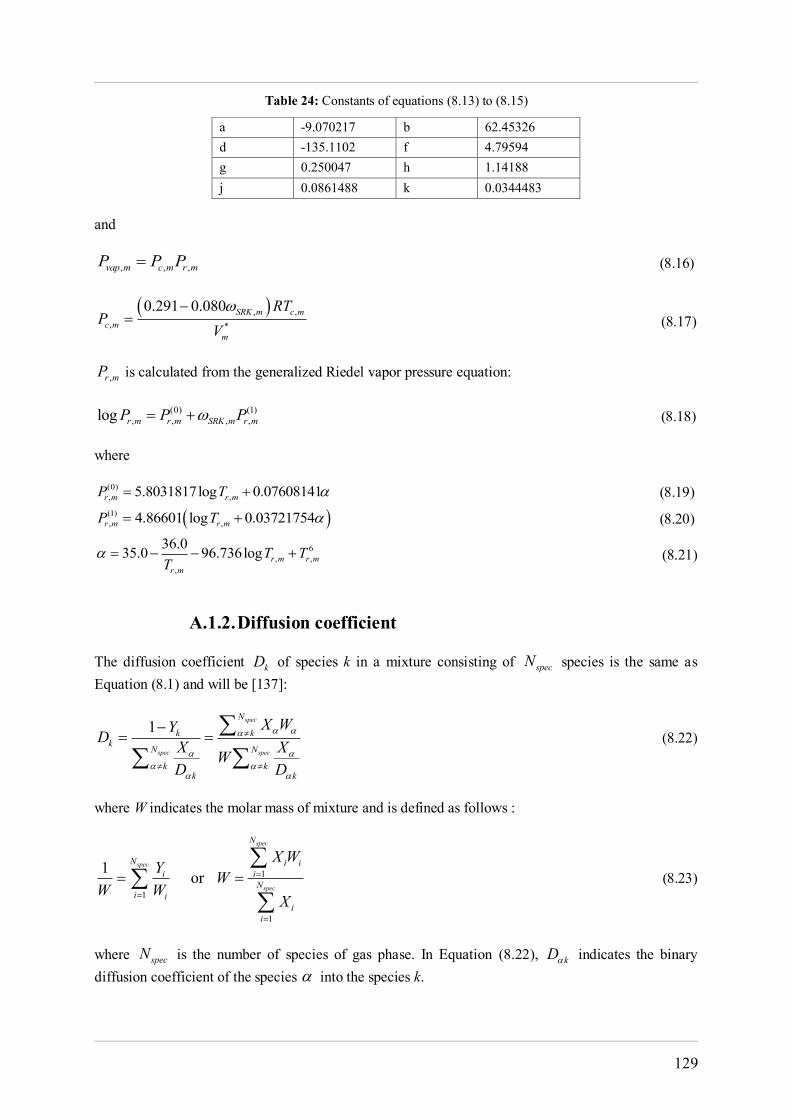
129
Table 24: Constants of equations (8.13) to (8.15)
a -9.070217 b 62.45326 d -135.1102 f 4.79594 g 0.250047 h 1.14188 j 0.0861488 k 0.0344483
and
, , ,vap m c m r mP P P (8.16)
, ,, *
0.291 0.080 SRK m c mc m
m
RTP
V
(8.17)
,r mP is calculated from the generalized Riedel vapor pressure equation:
(0) (1)
, , , ,log r m r m SRK m r mP P P (8.18) where
(0), ,5.8031817log 0.07608141r m r mP T (8.19)
(1), ,4.86601 log 0.03721754r m r mP T (8.20)
6, ,
,
36.035.0 96.736log r m r mr m
T TT
(8.21)
A.1.2. Diffusion coefficient The diffusion coefficient kD of species k in a mixture consisting of specN species is the same as Equation (8.1) and will be [137]:
1 spec
spec spec
N
k kk N N
k kk k
X WYD X XWD D
(8.22)
where W indicates the molar mass of mixture and is defined as follows :
1
1
1
1 or
spec
spec
spec
N
N i ii i
Ni i
ii
X WY W
W WX
(8.23)
where specN is the number of species of gas phase. In Equation (8.22), kD indicates the binary diffusion coefficient of the species into the species k.

130
Several methods for estimating kD in binary gas systems were proposed by some authors.
Hirschfelder et al. [125] suggested a model to obtain the diffusion coefficient for binary and multi-component mixture. In their model, the binary diffusion coefficients are given in terms of pressure and temperature. Shapiro [243] derived general expressions for diffusion coefficients in multi-component non-ideal gas or liquid mixtures. The derivation is based on the general statistical theory of fluctuations around an equilibrium state. The matrix of diffusion coefficients is expressed in terms of the equilibrium thermodynamic characteristics of the mixture (such as molar densities and internal energy), as well as in terms of the newly introduced parameters, the penetration lengths. Gopalakrishnan and Abraham [123] considered the species and thermal diffusion coefficients as functions of temperature, pressure, and composition. They used an approximate method based on the mixture-average formulation to compute the species transport. Brück et al. [244] applied the method of Fuller et al. [245] to calculate the diffusion coefficient of ammonia in air. This method was also applied by Kawano et al. [246] to control the spray and combustion processes in internal combustion engine, using the multi-component fuel with high and low volatilities. Ra et al. [247] used Chapman-Enskog kinetic theory (Skelland [248]) on diesel engine combustion characteristics with bio-diesel fuels. The method of Fuller et al. [245] for the calculation of binary diffusion coefficient kD is given by:
1.75
21/3 1/31/ 2
0.00143k
k v v k
TDPW
(8.24)
where, T is the temperature (in K), W and kW are molecular weights of and k ( /g mol ), P is pressure (bar), kW is the average molar weight and v is found for each component by summing atomic diffusion volumes defined in Table 25 [245].
Table 25: Atomic Diffusion Volumes
Atomic and Structural Diffusion Volume Increments
C 15.9 F 14.7 H 2.31 Cl 21.0 O 6.11 Br 21.9 N 4.54 I 29.8
Aromatic ring -18.3 S 22.9 Heterocyclic ring -18.3
Diffusion Volumes of Simple Molecules
He 2.67 CO 18.0 Ne 5.98 CO2 26.9 Ar 16.2 N2O 35.9 Kr 24.5 NH3 20.7 Xe 32.7 H2O 13.1 H2 6.12 SF6 71.3 D2 6.84 Cl2 38.4 N2 18.5 Br2 69.0 O2 16.3 SO2 41.8 Air 19.7
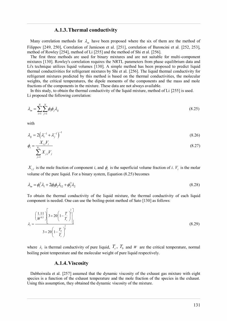
131
A.1.3. Thermal conductivity Many correlation methods for m have been proposed where the six of them are the method of Filippov [249, 250], Correlation of Jamieson et al. [251], correlation of Baroncini et al. [252, 253], method of Rowley [254], method of Li [255] and the method of Shi et al. [256]. The first three methods are used for binary mixtures and are not suitable for multi-component mixtures [130]. Rowley's correlation requires the NRTL parameters from phase equilibrium data and Li's technique utilizes liquid volumes [130]. A simple method has been proposed to predict liquid thermal conductivities for refrigerant mixtures by Shi et al. [256]. The liquid thermal conductivity for refrigerant mixtures predicted by this method is based on the thermal conductivities, the molecular weights, the critical temperatures, the dipole moments of the components and the mass and mole fractions of the components in the mixture. These data are not always available. In this study, to obtain the thermal conductivity of the liquid mixture, method of Li [255] is used. Li proposed the following correlation:
1 1
N N
m i j iji j
(8.25)
with
11 12ij i j
(8.26)
,
,1
L
i l ii N
j l jj
X V
X V
(8.27)
,i lX is the mole fraction of component i, and i is the superficial volume fraction of i. iV is the molar
volume of the pure liquid. For a binary system, Equation (8.25) becomes
2 21 1 1 2 12 2 22m (8.28)
To obtain the thermal conductivity of the liquid mixture, the thermal conductivity of each liquid component is needed. One can use the boiling-point method of Sato [130] as follows:
23
0.5
23
1.11 3 20 1
3 20 1
c
l
b
c
TTW
TT
(8.29)
where l is thermal conductivity of pure liquid, , c bT T and W are the critical temperature, normal boiling point temperature and the molecular weight of pure liquid respectively.
A.1.4. Viscosity Dabhoiwala et al. [257] assumed that the dynamic viscosity of the exhaust gas mixture with eight species is a function of the exhaust temperature and the mole fraction of the species in the exhaust. Using this assumption, they obtained the dynamic viscosity of the mixture.
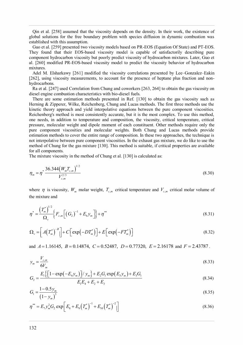
132
Qin et al. [258] assumed that the viscosity depends on the density. In their work, the existence of global solutions for the free boundary problem with species diffusion in dynamic combustion was established with this assumption. Guo et al. [259] presented two viscosity models based on PR-EOS (Equation Of State) and PT-EOS. They found that their EOS-based viscosity model is capable of satisfactorily describing pure component hydrocarbon viscosity but poorly predict viscosity of hydrocarbon mixtures. Later, Guo et al. [260] modified PR-EOS-based viscosity model to predict the viscosity behavior of hydrocarbon mixtures. Adel M. Elsharkawy [261] modified the viscosity correlations presented by Lee–Gonzalez–Eakin [262], using viscosity measurements, to account for the presence of heptane plus fraction and non-hydrocarbons. Ra et al. [247] used Correlation from Chung and coworkers [263, 264] to obtain the gas viscosity on diesel engine combustion characteristics with bio-diesel fuels. There are some estimation methods presented in Ref. [130] to obtain the gas viscosity such as Herning & Zipperer, Wilke, Reichenberg, Chung and Lucas methods. The first three methods use the kinetic theory approach and yield interpolative equations between the pure component viscosities. Reichenberg's method is most consistently accurate, but it is the most complex. To use this method, one needs, in addition to temperature and composition, the viscosity, critical temperature, critical pressure, molecular weight and dipole moment of each constituent. Other methods require only the pure component viscosities and molecular weights. Both Chung and Lucas methods provide estimation methods to cover the entire range of composition. In these two approaches, the technique is not interpolative between pure component viscosities. In the exhaust gas mixture, we do like to use the method of Chung for the gas mixture [130]. This method is suitable, if critical properties are available for all components. The mixture viscosity in the method of Chung et al. [130] is calculated as:
1/ 2
,*2/3,
36.344 m c mm
c m
W TV
(8.30)
where is viscosity, mW molar weight, ,c mT critical temperature and ,c mV critical molar volume of the mixture and
1/ 2*1* **
, 2 6m
c m mv
TF G E y
(8.31)
* * *exp expB
v m m mA T C DT E FT
(8.32)
and 1.16145,A 0.14874,B 0.52487,C 0.77320,D 2.16178E and 2.43787F .
,
6c m
mm
Vy
V (8.33)
1 4 2 1 5 3 12
1 4 2 3
1 exp / expm m mE E y y E G E y E GG
E E E E
(8.34)
1 3
1 0.51
m
m
yGy
(8.35)
1 2** 2 * *
7 2 8 9 10expm m mE y G E E T E T
(8.36)
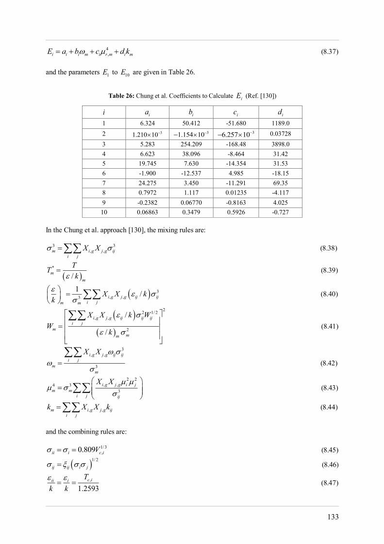
133
4,i i i m i r m i mE a b c d k (8.37)
and the parameters 1E to 10E are given in Table 26.
Table 26: Chung et al. Coefficients to Calculate iE (Ref. [130])
i ia ib ic id
1 6.324 50.412 -51.680 1189.0 2 31.210 10 31.154 10 36.257 10 0.03728 3 5.283 254.209 -168.48 3898.0 4 6.623 38.096 -8.464 31.42 5 19.745 7.630 -14.354 31.53 6 -1.900 -12.537 4.985 -18.15 7 24.275 3.450 -11.291 69.35 8 0.7972 1.117 0.01235 -4.117 9 -0.2382 0.06770 -0.8163 4.025
10 0.06863 0.3479 0.5926 -0.727 In the Chung et al. approach [130], the mixing rules are:
3 3, ,m i g j g ij
i jX X (8.38)
*
/mm
TTk
(8.39)
3, ,3
1 /i g j g ij iji jm m
X X kk
(8.40)
22 1/ 2, ,
2
/
/
i g j g ij ij iji j
mmm
X X k WW
k
(8.41)
3, ,
3
i g j g ij iji j
mm
X X
(8.42)
2 2, ,4 3
3i g j g i j
m mi j ij
X X
(8.43)
, ,m i g j g iji j
k X X k (8.44)
and the combining rules are:
1/3,0.809ii i c iV (8.45)
1/ 2
ij ij i j (8.46)
,
1.2593c iii i T
k k
(8.47)
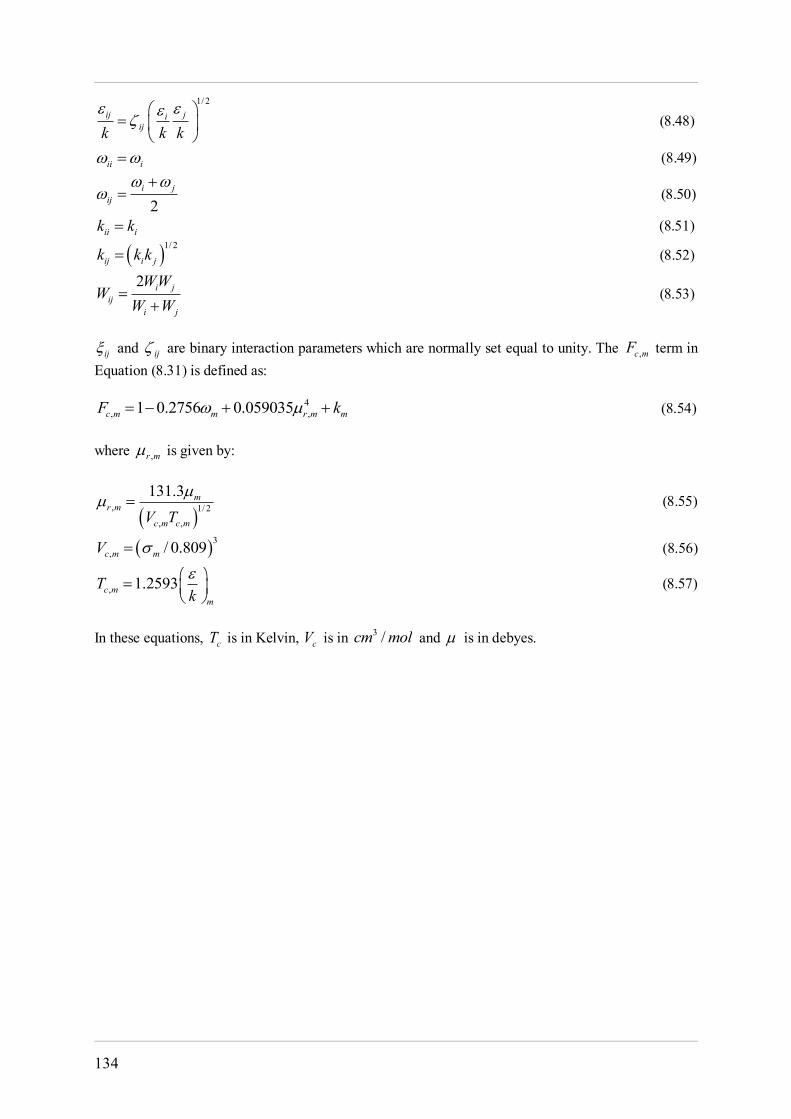
134
1/ 2ij ji
ijk k k
(8.48)
ii i (8.49)
2i j
ij
(8.50)
ii ik k (8.51)
1/ 2
ij i jk k k (8.52)
2 i jij
i j
WWW
W W
(8.53)
ij and ij are binary interaction parameters which are normally set equal to unity. The ,c mF term in
Equation (8.31) is defined as:
4, ,1 0.2756 0.059035c m m r m mF k (8.54)
where ,r m is given by:
, 1/ 2
, ,
131.3 mr m
c m c mV T
(8.55)
3
, / 0.809c m mV (8.56)
, 1.2593c mm
Tk
(8.57)
In these equations, cT is in Kelvin, cV is in 3 /cm mol and is in debyes.
135
Appendix B.
Vapor-Liquid Equilibrium At the liquid-gas interface, for every component i in the mixture, the condition of thermodynamic equilibrium is given by [130]:
v li if f (9.1)
where f is the fugacity. The exponents v and l stand for vapor and liquid phases respectively. The fugacity of a component in a mixture depends on the temperature, pressure and composition of that mixture. Reid et al. [130] introduced the fugacity coefficient i as follows:
ii
i
fX P
(9.2)
where Xi is the mole fraction of component i and P is the total pressure. Assuming a non-ideal solution, the surface mole fraction of the droplet can be determined using the thermodynamic equilibrium condition for the partial vaporization at the given temperature and pressure as [163]:
, , , ,s
i g i g i l i lX X (9.3) where the fugacity coefficients are evaluated from an equation of state. The two-parameter cubic equation of state is often used for hydrocarbon mixtures. It can be expressed by
2 2m
m m m
aRTPV b V kb V k b
. (9.4)
An equivalent form of Equation (9.4) is:
3 2 2 2 2 31 0Z B kB Z A k B kB kB Z A B k B k B (9.5) where
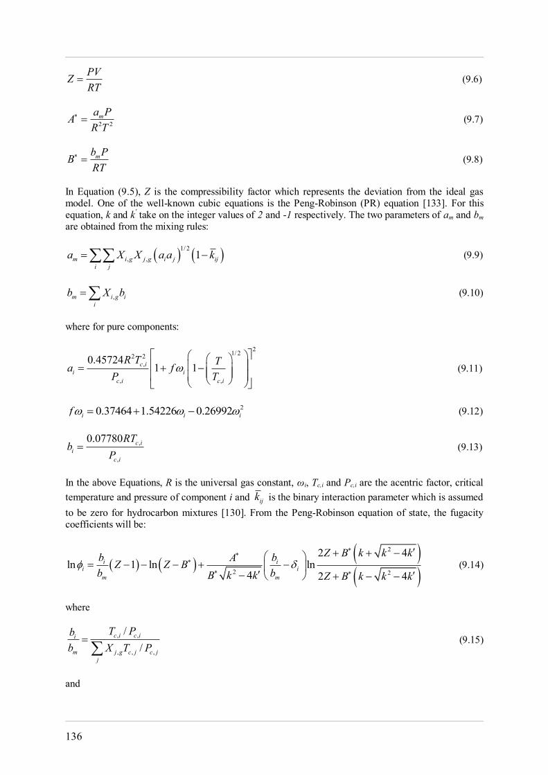
136
PVZRT
(9.6)
2 2ma PA
R T (9.7)
mb PB
RT (9.8)
In Equation (9.5), Z is the compressibility factor which represents the deviation from the ideal gas model. One of the well-known cubic equations is the Peng-Robinson (PR) equation [133]. For this equation, k and k' take on the integer values of 2 and -1 respectively. The two parameters of am and bm are obtained from the mixing rules:
1/ 2
, , 1m i g j g i j iji j
a X X a a k (9.9)
,m i g ii
b X b (9.10)
where for pure components:
21/ 22 2,
, ,
0.457241 1c i
i ic i c i
R T Ta fP T
(9.11)
20.37464 1.54226 0.26992i i if (9.12)
,
,
0.07780 c ii
c i
RTb
P (9.13)
In the above Equations, R is the universal gas constant, ωi, Tc,i and Pc,i are the acentric factor, critical temperature and pressure of component i and ijk is the binary interaction parameter which is assumed to be zero for hydrocarbon mixtures [130]. From the Peng-Robinson equation of state, the fugacity coefficients will be:
2
2 2
2 4ln 1 ln ln
4 2 4i i
i im m
Z B k k kb bAZ Z Bb bB k k Z B k k k
(9.14)
where
, ,
, , ,
//
c i c ii
m j g c j c jj
T Pbb X T P
(9.15)
and
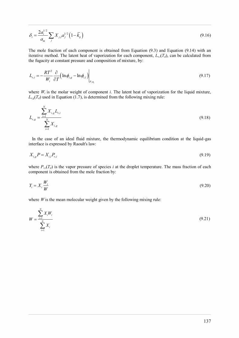
137
1/ 2
1/ 2,
2 1ii j l j ij
jm
a X a ka
(9.16)
The mole fraction of each component is obtained from Equation (9.3) and Equation (9.14) with an iterative method. The latent heat of vaporization for each component, Lv,i(Td), can be calculated from the fugacity at constant pressure and composition of mixture, by:
2
, , ,,
ln lni
v i i g i li P n
RTLW T
(9.17)
where Wi is the molar weight of component i. The latent heat of vaporization for the liquid mixture, Lv,g(Td) used in Equation (1.7), is determined from the following mixing rule:
, ,1
,
,1
N
i g v ii
v g N
i gi
X LL
X
(9.18)
In the case of an ideal fluid mixture, the thermodynamic equilibrium condition at the liquid-gas interface is expressed by Raoult's law:
, , ,i g i l v iX P X P (9.19) where Pv,i(Td) is the vapor pressure of species i at the droplet temperature. The mass fraction of each component is obtained from the mole fraction by:
ii i
WY XW
(9.20)
where W is the mean molecular weight given by the following mixing rule:
1
1
N
i ii
N
ii
X WW
X
(9.21)
138
Appendix C.
Hirschfelder's law by mass fraction
gradient The Hirschfelder's law for multi-species gas is as follows [125, 127, 134]:
i i im iV X D X (10.1) Considering the following relation between the mole and mass fraction of a species i :
i ii
WX YW
(10.2)
one can rewrite Equation (10.1) as:
1
i i ii i
WX Y WYW W
(10.3)
In Equation (10.3), W is the molar weight of the gas mixture which is a function of mass fraction of all species in the gas. For the species with close molar weights, it may be a good approximation to assume that the molar weight of gas mixture is constant. In this case, W exits from the definition of mass fraction gradient. In order to use the Hirschfelder's law for the species with different molar weights, the molar weight of gas mixture could not be constant. Thus, a new expression for the Hirschfelder's law is needed. For the binary mixture, we assume that the molar weight of mixture is expressed as:
1 2 1 1
1 2 1 2
11 Y Y Y YW W W W W
(10.4)
thus,
1 2
1 2 1 11WWW
YW Y W
(10.5)
139
Substituting Equation (10.5) into Equation (10.3) for binary mixture gives:
1
1 21 2 1 11
YX WYW Y W
(10.6)
The right hand side of the above Equation can be written as:
1 2 1 1
1 2 12 21 2 1 1 1 2 1 1 1 2 1 1
11 1 1
YW YWX W YYW Y W YW Y W YW Y W
(10.7)
Multiplying the numerator and denominator of the first part of Equation (10.7) with 1W , the second
part with 21W and the third part with 1 2WW , one obtains:
2 2 2 21 2 1 1 2 1 1 2
1 12 221 1 2 1 1 1 1 2 1 1 1 2 1 2 1 1
1 1 1WW YW W YW WX Y
W YW Y W W YW Y W WW YW Y W
(10.8)
Rewriting Equation (10.5) in the following form:
1 2 1 2 1 1
11
WWW YW Y W
(10.9)
and substituting Equation (10.9) into Equation (10.8) gives:
2 21 1
1 121 1 1 2
YW YWWX YW W WW
(10.10)
Coming back to the first Equation (10.1), one can rewrite the Hirschfelder's law for binary system using Equation (10.2) and (10.10):
2 21 1
1 1 1 121 1 1 1 2
mYW YWW WVY D Y
W W W WW
(10.11)
or in the simplified form:
21 1 1 1 1 1
2
1mXVY D X Y YY
(10.12)
Substituting Equation (8.22) (from Section A.1.2) for the binary system:
2 21
2
12
mX WD XW
D
(10.13)
into Equation (10.12) gives the Fick's law for the binary system:
140
1 1 12 1VY D Y (10.14)
The same procedure for multispecies system gives the following expression for the Hirschfelder's law as:
11
Nk
i i im i i ik kk i
XVY D X Y YY
(10.15)
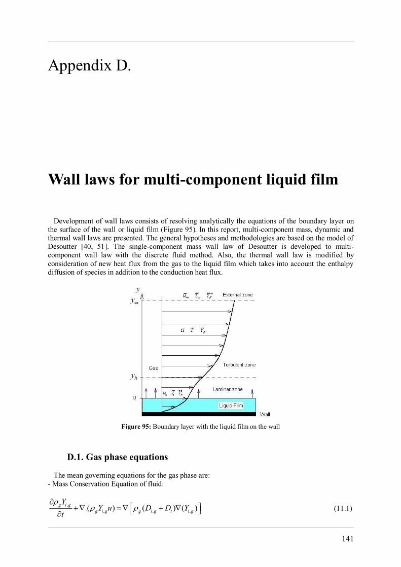
141
Appendix D.
Wall laws for multi-component liquid film Development of wall laws consists of resolving analytically the equations of the boundary layer on the surface of the wall or liquid film (Figure 95). In this report, multi-component mass, dynamic and thermal wall laws are presented. The general hypotheses and methodologies are based on the model of Desoutter [40, 51]. The single-component mass wall law of Desoutter is developed to multi-component wall law with the discrete fluid method. Also, the thermal wall law is modified by consideration of new heat flux from the gas to the liquid film which takes into account the enthalpy diffusion of species in addition to the conduction heat flux.
Figure 95: Boundary layer with the liquid film on the wall
D.1. Gas phase equations The mean governing equations for the gas phase are: - Mass Conservation Equation of fluid:
,, , ,.( ) ( ) ( )g i g
g i g g i g t i g
YY u D D Y
t
(11.1)
142
where ,,
mi g
l i
DSc
and tt
t
DSc
represent the laminar and turbulent diffusion coefficients
respectively and i denotes the components of fluid. - Mass Conservation Equation for the mixed gases:
.( ) 0ggut
(11.2)
- Conservation Equation of the Movement of the gas:
.( ) .gg g
uuu p g
t
(11.3)
where represents the shear tensor, and g the gravity acceleration. - Conservation Equation of the energy I of the gas:
.( ) . .gg
I pIu u p Jt t
(11.4)
where J represents the heat flux vector and generally defined as /m m
mJ T D h .
D.2. Hypothesis of resolution To develop the wall laws, classical hypotheses mentioned in section 2.3, will be used. First, we assume that the gas is incompressible.
D.3. Mass conservation of the gas Applying the mentioned hypotheses, mass conservation equation of the gas (Equation (11.2)) will be:
0gvy
(11.5)
Specific mass evaporation rate gm v is constant in the normal direction of liquid film in the boundary layer. As it is supposed that the gas is incompressible, the normal velocity to the film v is constant in y direction and is equal to Stephan velocity sv .
D.4. Mean movement conservation Using the mentioned hypotheses, conservation equation of the mean movement (Equation (11.3)) will be:
143
. ( )m tu v uy y y
(11.6)
where t is turbulent viscosity that could be modeled according to the Prandtl mixing-length theory:
2( )tukyy
(11.7)
where k indicates the Karmann's constant. After integration, one obtains:
2
1. s mu uu v ky Ky y
(11.8)
where 1K indicates a constant of integration determined with the boundary condition for the tangential velocity of the gas on the surface of the film ( 0) su y u and for its normal gradient
, 2
,
g sm
g ss
u uy
.
The non-dimensional coordinate y is defined using the characteristic length scale , /m s u where
u and ,m s are respectively the shear velocity and the laminar kinematical viscosity of the gas at the liquid film surface.
,m s
yuy
(11.9)
Equation (11.8) is written in dimensionless form as:
2 21 1su uu v k yy y
(11.10)
where , su v and T are defined as follow (T will be used in the next sections):
su uuu
(11.11)
ss
vvu
(11.12)
,
,
( )s g s p
g s
T T C uT
(11.13)
where pC and ,g s are respectively the mass specific heat capacity at constant pressure for the mixture and the heat flux between the gas flow and the film at the liquid-gas interface.
144
D.4.1. Inertial turbulent sub-layer In the inertial sub-layer, laminar viscosity of the gas g is negligible against the turbulent viscosity
t . Thus, Equation (11.10) reduces to:
22 21 s
uu v k yy
(11.14)
Equation (11.14) could be rewritten as:
1 suu v kyy
(11.15)
A new integration in the inertial sub-layer, i.e. from lty to y , gives the following relation:
1lt lt
yu
u ys
du dykyu v
(11.16)
where ltu indicates the dimensionless transversal velocity of the gas on the laminar-turbulence transition. Thus, one obtains: 2 11 1 lns lt ss lt
yu v u vv k y
(11.17)
D.4.2. Laminar sub-layer
In the laminar sub-layer, turbulent viscosity t is negligible against laminar viscosity of the gas m . Thus, Equation (11.10) reduces to:
1 suu vy
(11.18)
After integration, one obtains the mean dimensionless transversal velocity u in the laminar sub-layer:
21
sv y
s
u K ev
(11.19)
where 2K is a constant of integration.
Besides, on the surface of the liquid film, the mean dimensionless transversal velocity su is zero. Consequently, in the laminar sub-layer, one theoretically has:
1 1sv y
s
u ev
(11.20)
145
or
22 21sv y
ss s
u v ev v
(11.21)
Finally, Equation (11.21) can be replaced with the following equation in which the new effective variable effU for the dynamics wall laws appears:
2 1 1eff ss
U u v yv
(11.22)
D.4.3. Assessment
An expression of the mean dimensionless transversal velocity at the laminar-turbulent transition ltu can be obtained. Substituting Equation (11.22) in to Equation (11.17) gives an expression for the new effective variable effU in the inertial turbulent sub-layer. Equation (11.22) supplies expression of effU in the laminar sub-layer. The following dynamics wall laws can then be obtained before accounting the compressibility of the gas:
2: 1 1
2 1: 1 1 ln
lt eff ss
lt eff s lts lt
y y U u v yv
yy y U u v yv k y
(11.23)
D.5. Mass conservation of liquid
By applying the previous hypotheses, equation of mean mass conservation of liquid, (Equation (11.1)), is:
, ,,
.( )i g i g
i g t
vY YD D
y y y
(11.24)
where tD and ,i gD respectively can express themselves to find the turbulent Schmidt number of the
gas tt
t
DSc
and the laminar Schmidt number of the liquid-gas ,i gD . Contrary to the droplet
modeling, using the corrected Stephan velocity in the mass conservation equation makes it very difficult to integrate the mass conservation equation in the film modeling. To consider this corrected velocity and to overcome this problem, a laminar Schmidt number is introduced. A first integration leads to:
2 2, ,
, , 1, ,
. .i g i gm t ms i g s i g
l i t l i t
Y Yk y uv Y v Y KSc Sc y Sc Sc y y
(11.25)
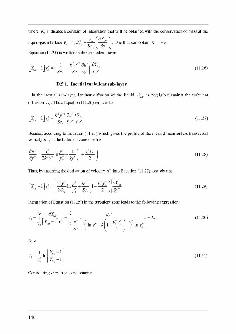
146
where 1K indicates a constant of integration that will be obtained with the conservation of mass at the
liquid-gas interface ,,
,
. i gs ms s i g
l i s
Yv v Y
Sc y
. One thus can obtain 1 sK v .
Equation (11.25) is written in dimensionless form:
2 2,
,,
11 i gi g s
l i t
Yk y uY vSc Sc y y
(11.26)
D.5.1. Inertial turbulent sub-layer
In the inertial sub-layer, laminar diffusion of the liquid ,i gD is negligible against the turbulent
diffusion tD . Thus, Equation (11.26) reduces to:
2 2,
, 1 i gi g s
t
Yk y uY vSc y y
(11.27)
Besides, according to Equation (11.23) which gives the profile of the mean dimensionless transversal velocity u , in the turbulent zone one has:
2
1ln 12 2
s s lt
lt
v v yu yy k y y ky
(11.28)
Thus, by inserting the derivation of velocity u into Equation (11.27), one obtains:
,, 1 ln 1
2 2i gs s lt
i g st lt t
Yv y v yy kyY vSc y Sc y
(11.29)
Integration of Equation (11.29) in the turbulent zone leads to the following expression:
,
,
,1 2
, 1ln 1 ln
2 2 2
i g
lti g lt
Y yi g
i g sY y s s lt slt
t
dY dyI IY v v v y vy y k y
Sc
. (11.30)
Now,
,1
,
11 ln1
i glt
s i g
YI
v Y
(11.31)
Considering ln y , one obtains:
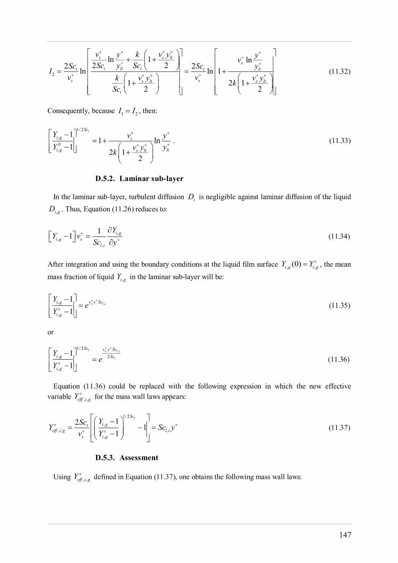
147
2
ln 1 ln2 22 2ln ln 1
1 2 12 2
s s lts
t lt tt t lt
s ss lt s lt
t
v v yy k yvSc y ScSc Sc yI
v vv y v yk kSc
(11.32)
Consequently, because 1 2I I , then:
1/ 2
,
,
11 ln
12 1
2
tSc
i g slt
i g lts lt
Y v yY yv yk
. (11.33)
D.5.2. Laminar sub-layer
In the laminar sub-layer, turbulent diffusion tD is negligible against laminar diffusion of the liquid
,i gD . Thus, Equation (11.26) reduces to:
,,
,
11 i gi g s
l i
YY v
Sc y
(11.34)
After integration and using the boundary conditions at the liquid film surface , ,(0) s
i g i gY Y , the mean
mass fraction of liquid ,i gY in the laminar sub-layer will be:
,,
,
11
s l iv y Sci gs
i g
Ye
Y
(11.35)
or
,1/ 2
, 2
,
11
t s l i
t
Sc v y Sci g Scs
i g
Ye
Y
(11.36)
Equation (11.36) could be replaced with the following expression in which the new effective variable , ,eff i gY for the mass wall laws appears:
1/ 2
,, , ,
,
12 11
tSc
i gteff i g l is
s i g
YScY Sc yv Y
(11.37)
D.5.3. Assessment
Using , ,eff i gY defined in Equation (11.37), one obtains the following mass wall laws:
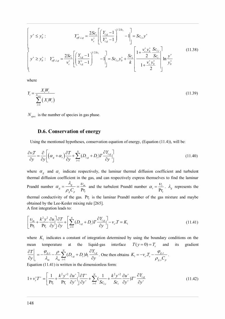
148
1/ 2
,, , ,
,
,1/ 2
,, , ,
,
12: 11
112 2: 1 ln1 1
2
t
t
Sc
i gtlt eff i g l is
s i g
l is ltSc
i gt t tlt eff i g l i lts
s lts i g lt
YScy y Y Sc yv Y
Scv yYSc Sc Sc yy y Y Sc y
v yv Y k y
(11.38)
where
1
spec
i ii N
i ii
X WYX W
(11.39)
specN is the number of species in gas phase.
D.6. Conservation of energy Using the mentioned hypotheses, conservation equation of energy, (Equation (11.4)), will be:
,,
1
. ( )N
i gg t i g t
i
YvT T D D Ty y y y
(11.40)
where g and t indicate respectively, the laminar thermal diffusion coefficient and turbulent thermal diffusion coefficient in the gas, and can respectively express themselves to find the laminar
Prandtl number Pr
g mg
g p lC
and the turbulent Prandtl number Pr
tt
t
. g represents the
thermal conductivity of the gas. Prl is the laminar Prandtl number of the gas mixture and maybe obtained by the Lee-Kesler mixing rule [265]. A first integration leads to:
2 2,
, 11
( ) .Pr Pr
Ni gm
i g t sil t
Yk y u T D D T v T Ky y y
(11.41)
where 1K indicates a constant of integration determined by using the boundary conditions on the mean temperature at the liquid-gas interface ( 0) sT y T and its gradient
, ,,
1( )
Ng s i g
i g t iim ms
YT D D hy y
. One then obtains ,
1,
. g ss s
g s p
K v TC
.
Equation (11.41) is written in the dimensionless form:
2 2 2 2,
1 ,
1 11 ( )Pr Pr
Ni g
sil t l i t
Yk y u T k y uv T Ty y Sc Sc y y
(11.42)
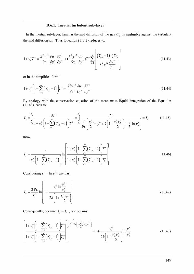
149
D.6.1. Inertial turbulent sub-layer In the inertial sub-layer, laminar thermal diffusion of the gas g is negligible against the turbulent
thermal diffusion t . Thus, Equation (11.42) reduces to:
2 2 2 2,
2 21
11 ( )
Pr
Ni g s t
sit t
Y v Sck y u T k y uv T Tuy y Sc y k yy
(11.43)
or in the simplified form:
2 2
,1
1 1 1Pr
N
s i gi t
k y u Tv Y Ty y
(11.44)
By analogy with the conservation equation of the mean mass liquid, integration of the Equation (11.43) leads to:
3 4
,1
1 1 1 ln 1 lnPr 2 2 2
lt lt
yT
NT y s s lt s
s i g lti t
dT dyI Iv v y vyv Y T y k y
(11.45)
now,
,1
3
, ,1 1
1 1 11 ln
1 1 1 1 1
N
s i gi
N N
s i g s i g lti i
v Y TI
v Y v Y T
(11.46)
Considering ln y , one has:
4
ln2Pr ln 1
2 12
st lt
s s lt
yvyI
v v yk
(11.47)
Consequently, because 3 4I I , one obtains:
,1
1
2Pr 1 1,
1
,1
1 1 11 ln
1 1 1 2 12
N
t i gi
NY
s i gi sN
lts lts i g lt
i
v Y Tv y
yv yv Y T k
(11.48)
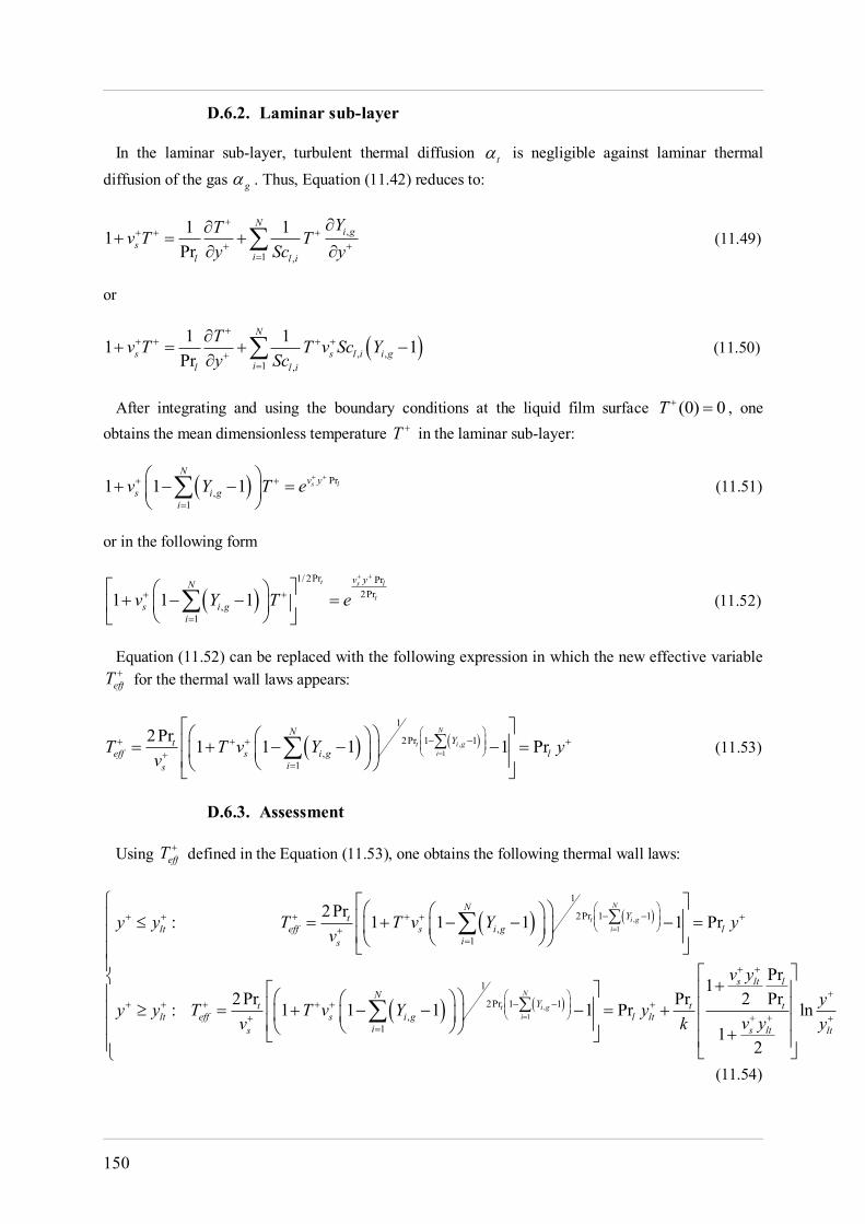
150
D.6.2. Laminar sub-layer In the laminar sub-layer, turbulent thermal diffusion t is negligible against laminar thermal
diffusion of the gas g . Thus, Equation (11.42) reduces to:
,
1 ,
1 11Pr
Ni g
sil l i
YTv T Ty Sc y
(11.49)
or
, ,1 ,
1 11 1Pr
N
s s l i i gil l i
Tv T T v Sc Yy Sc
(11.50)
After integrating and using the boundary conditions at the liquid film surface (0) 0T , one obtains the mean dimensionless temperature T in the laminar sub-layer:
Pr,
11 1 1 s l
Nv y
s i gi
v Y T e
(11.51)
or in the following form
1/ 2Pr Pr
2Pr,
11 1 1
t s l
t
v yN
s i gi
v Y T e
(11.52)
Equation (11.52) can be replaced with the following expression in which the new effective variable
effT for the thermal wall laws appears:
,1
1
2Pr 1 1,
1
2Pr 1 1 1 1 PrN
t i gi
NYt
eff s i g lis
T T v Y yv
(11.53)
D.6.3. Assessment
Using effT defined in the Equation (11.53), one obtains the following thermal wall laws:
,1
,1
1
2Pr 1 1,
1
1
2Pr 1 1,
1
2Pr: 1 1 1 1 Pr
12Pr Pr: 1 1 1 1 Pr
N
t i gi
N
t i gi
NYt
lt eff s i g lis
NYt t
lt eff s i g l ltis
y y T T v Y yv
v
y y T T v Y yv k
Pr2 Pr ln
12
s lt l
t
s lt lt
yy
v y y
(11.54)
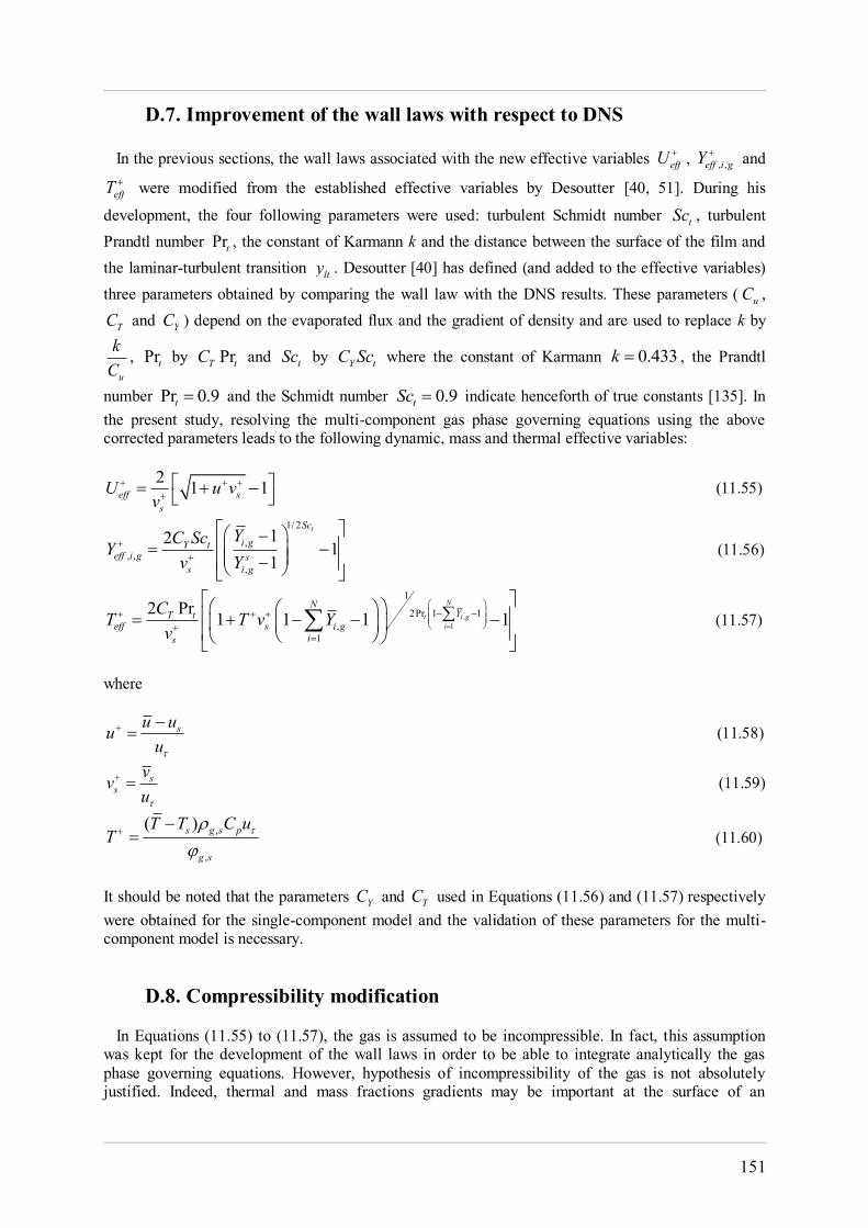
151
D.7. Improvement of the wall laws with respect to DNS In the previous sections, the wall laws associated with the new effective variables effU , , ,eff i gY and
effT were modified from the established effective variables by Desoutter [40, 51]. During his
development, the four following parameters were used: turbulent Schmidt number tSc , turbulent Prandtl number Prt , the constant of Karmann k and the distance between the surface of the film and the laminar-turbulent transition lty . Desoutter [40] has defined (and added to the effective variables) three parameters obtained by comparing the wall law with the DNS results. These parameters ( uC ,
TC and YC ) depend on the evaporated flux and the gradient of density and are used to replace k by
u
kC
, Prt by PrT tC and tSc by Y tC Sc where the constant of Karmann 0.433k , the Prandtl
number Pr 0.9t and the Schmidt number 0.9tSc indicate henceforth of true constants [135]. In the present study, resolving the multi-component gas phase governing equations using the above corrected parameters leads to the following dynamic, mass and thermal effective variables:
2 1 1eff ss
U u vv
(11.55)
1/ 2
,, ,
,
12 11
tSc
i gY teff i g s
s i g
YC ScYv Y
(11.56)
,1
1
2Pr 1 1,
1
2 Pr 1 1 1 1N
t i gi
NYT t
eff s i gis
CT T v Yv
(11.57)
where
su uuu
(11.58)
ss
vvu
(11.59)
,
,
( )s g s p
g s
T T C uT
(11.60)
It should be noted that the parameters YC and TC used in Equations (11.56) and (11.57) respectively were obtained for the single-component model and the validation of these parameters for the multi-component model is necessary.
D.8. Compressibility modification In Equations (11.55) to (11.57), the gas is assumed to be incompressible. In fact, this assumption was kept for the development of the wall laws in order to be able to integrate analytically the gas phase governing equations. However, hypothesis of incompressibility of the gas is not absolutely justified. Indeed, thermal and mass fractions gradients may be important at the surface of an
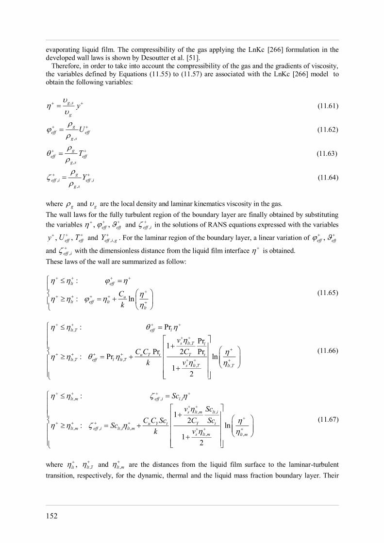
152
evaporating liquid film. The compressibility of the gas applying the LnKc [266] formulation in the developed wall laws is shown by Desoutter et al. [51]. Therefore, in order to take into account the compressibility of the gas and the gradients of viscosity, the variables defined by Equations (11.55) to (11.57) are associated with the LnKc [266] model to obtain the following variables:
,g s
g
y
(11.61)
,
geff eff
g s
U
(11.62)
,
geff eff
g s
T
(11.63)
, ,,
geff i eff i
g s
Y
(11.64)
where g and g are the local density and laminar kinematics viscosity in the gas. The wall laws for the fully turbulent region of the boundary layer are finally obtained by substituting the variables , ,eff
eff and ,eff i in the solutions of RANS equations expressed with the variables
,y ,effU
effT and , ,eff i gY . For the laminar region of the boundary layer, a linear variation of ,eff
eff
and ,eff i with the dimensionless distance from the liquid film interface is obtained. These laws of the wall are summarized as follow:
:
: ln
lt eff
ult eff lt
lt
Ck
(11.65)
,
,
, ,, ,
: Pr
Pr1Pr 2 Pr: Pr ln
12
lt T eff l
s lt T l
u T t T tlt T eff l lt T
s lt T lt T
vC C C
vk
(11.66)
, , ,
, ,
, , , ,, ,
:
12: ln
12
lt m eff i l i
s lt m lt i
u Y t Y tlt m eff i lt i lt m
s lt m lt m
Sc
v ScC C Sc C ScSc
vk
(11.67)
where ,lt ,lt T and ,lt m are the distances from the liquid film surface to the laminar-turbulent transition, respectively, for the dynamic, thermal and the liquid mass fraction boundary layer. Their
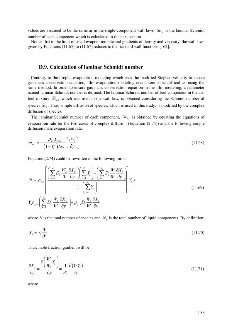
153
values are assumed to be the same as in the single-component wall laws. ,l iSc is the laminar Schmidt number of each component which is calculated in the next section. Notice that in the limit of small evaporation rate and gradients of density and viscosity, the wall laws given by Equations (11.65) to (11.67) reduces to the standard wall functions [162].
D.9. Calculation of laminar Schmidt number Contrary to the droplet evaporation modeling which uses the modified Stephan velocity to ensure gas mass conservation equation, film evaporation modeling encounters some difficulties using the same method. In order to ensure gas mass conservation equation in the film modeling, a parameter named laminar Schmidt number is defined. The laminar Schmidt number of fuel component in the air-fuel mixture ,l iSc which was used in the wall law, is obtained considering the Schmidt number of species iSc . Thus, simple diffusion of species, which is used in this study, is modified by the complex diffusion of species. The laminar Schmidt number of each component, ,l iSc is obtained by equating the equations of evaporation rate for the two cases of complex diffusion (Equation (2.74)) and the following simple diffusion mass evaporation rate:
, ,
,,1
g s g s ip i s
i l i s
YmyY Sc
(11.68)
Equation (2.74) could be rewritten in the following form:
1 1 1,
1
, ,1
1
l l
l
N NNk k i i
k i ik i i
i g s iN
ii
Nk k i i
i g s k g s ik
W X W XD Y DW y W y
m YY
W X W XY D DW y W y
(11.69)
where N is the total number of species and lN is the total number of liquid components. By definition:
i ii
WX YW
(11.70)
Thus, mole fraction gradient will be:
1ii ii
i
W YW WYX
y y W y
(11.71)
where
154
1
1 Nk
k k
YW W
(11.72)
or
1 1
1 1N N
k i k
k kk i kk i
WY Y YW W W
. (11.73)
By introducing A as:
1
Na
a aa i
YAW
(11.74)
then,
1i
i
W Y AW
(11.75)
or,
i
i
WWY A
(11.76)
Then, Equation (11.71) can be rewritten as:
2
1 1i
i iii i i
i i i i i
YY AWWYX Y Y
y W y y Y AW yY AW
(11.77)
Considering:
,g sk
k
DSc
(11.78)
we have the following equality:
155
21 1
1
21
1
1
1
1
1
1
1
1 1
l
l
l
l
NNk k k
ik ik k k k k
iN
ii
Ni i i
i i i i i i
N
ii
ki
k k k
W Y Y YSc Y AW yY AW
YW
Y
W Y YSc Y AW yY AW
WY
WYW Sc Y AW
21
2,
1 1 11
Nk k
k k k
i i i i
i i i i l ii i
Y YyY AW
W Y Y YW Sc Y AW y Y Sc yY AW
(11.79) Thus, for each component in the liquid,
,
1 1 1
1
1
11
l l
l
l i N NN
i k i Ni k i
i i i k iNk
ii
WSc
Y B BY Y Y B B
Y
(11.80)
where
2
1 , k kk
k k k k k
W Y AB k i
Sc Y AW Y AW
(11.81)
2
1i ii
i i i i i
W Y AB
Sc Y AW Y AW
(11.82)
and the following parameters are introduced in order to remove the mass fraction gradients:
1, or
N YA k i
W
(11.83)
1
1 11 , ,N
ki
A W i kW W
(11.84)
1
11 , N
iA W iW
(11.85)
156
Appendix E
IFP-C3D code
E.1. General description of IFP-C3D code IFP-C3D code is an unstructured parallel solver dedicated to the computation of multi-phase compressible turbulent flows including phase changes, mixture preparation and combustion, especially in automobile engines. IFP-C3D uses Arbitrary Lagrangian Eulerian (ALE) formalism with a finite volume method on staggered grids, time splitting, SIMPLE algorithm and sub-cycled advection. IFP-C3D is parallelized using the Message Passing Interface (MPI) library to distribute calculation over a large number of processors. Moreover, it uses an optimized linear algebraic library to solve linear matrix systems and the METIS partitioning library to distribute the computational load equally for all meshes used during the calculation. Main physical models included in IFP-C3D for liquid spray modeling are the multi-component evaporation model [145], the Wave-FIPA breakup model [166], the spray-wall interaction models including liquid film transport, evaporation [29, 51, 267, 268] and boiling [152]. For combustion modeling, IFP-C3D includes the auto-ignition TKI model [167], the spark plug ignition AKTIM model [168], the ECFM gasoline combustion model [269] and the ECFM3Z Diesel combustion model [169].
E.2. Description of the structure of IFP-C3D code The combustion code, IFP-C3D, solves the Navier-Stokes Multi-species hexahedral unstructured mobile meshes. The calculation cycle is decomposed temporally into three phases. Phase A, comprising the source terms related to chemistry, evaporation of liquid fuel (spray or film) and spark ignition (AKTIM Lagrangian model and a phenomenological model). It's more in this phase that the Lagrangian spray is treated (convection, atomization). In phase B, called Lagrangian phase, mesh nodes are moving at the speed of the fluid and there is no convection cells at the border of calculation. The different scattering terms and the terms of spreading pressure wave are solved implicitly. Coupled implicit equations are solved by the SIMPLE method and the linear systems involved are inverted using a library of linear algebra developed by IFP for the pressure solver or an iterative conjugate gradient for other variables. In phase C, called Eulerian, the convection terms are solved explicitly. A sub-cycling allows overcoming the stability condition (CFL < 1) inherent to all explicit methods. The system is solved using an explicit second order spatial pattern centered, QSOU, used with a limiter to preserve the monotony. The general algorithm of IFP-C3D code is presented below:
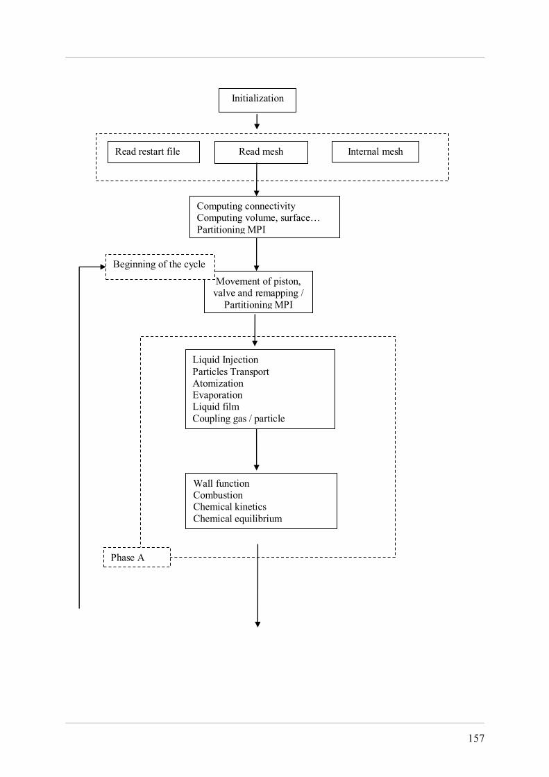
157
Initialization
Read mesh Internal mesh
Computing connectivity Computing volume, surface… Partitioning MPI
Read restart file
Movement of piston, valve and remapping /
Partitioning MPI
Liquid Injection Particles Transport Atomization Evaporation Liquid film Coupling gas / particle
Wall function Combustion Chemical kinetics Chemical equilibrium
Phase A
Beginning of the cycle
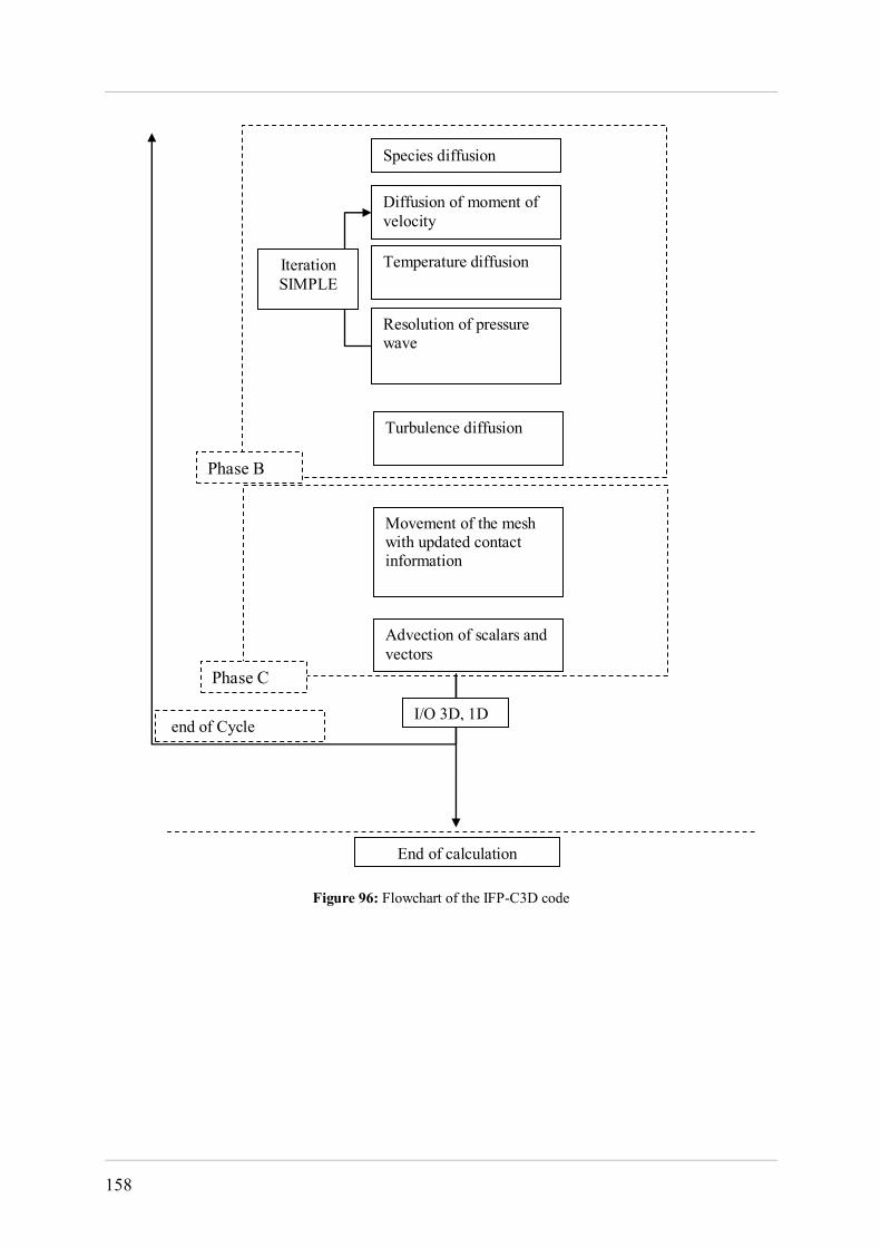
158
Figure 96: Flowchart of the IFP-C3D code
Species diffusion
Diffusion of moment of velocity
Temperature diffusion
Resolution of pressure wave
Iteration SIMPLE
Turbulence diffusion
Movement of the mesh with updated contact information
Advection of scalars and vectors
Phase C
Phase B
End of calculation
I/O 3D, 1D end of Cycle
159
Bibliography
[1] HEYWOOD J.B., Internal combustion engine fundamentals, New York, 1988.
[2] STONE R., Introduction to internal combustion engines, London, 1999.
[3] PERRIN H., DUMAS J.P., LAGET O. and WALTER B., Analysis of Combustion Process in Cold Operation with a Low Compression Ratio Diesel Engine, SAE International Journal of Engines, 3,1, pp.1012-1032, 2010.
[4] WALTER B., PERRIN H., DUMAS J.P. and LAGET O., Cold Operation with Optical and Numerical Investigations on a Low Compression Ratio Diesel Engine, SAE International Journal of Engines, 2,2, pp.186-204, 2009.
[5] E.W.CURTIS, A.ULUDOGAN and R.D.REITZ, A New High Pressure Droplet Vaporization Model for Diesel Engine Modeling, SAE Paper No. 952431, 1995.
[6] YIM S.D., KIM S.J., BAIK J.H., NAM I.S., MOK Y.S., LEE J.H., CHO B.K. and OH S.H., Decomposition of Urea into NH3 for the SCR Process, Ind.Eng.Chem.Res., 43, pp.4856-4863, 2004.
[7] ITAYA Y., DEGUCHI S., TAKEI M, YOSHINO M, MATSUDA H. and HASATANI M., NO reduction behavior by urea solution injection in the tubular reactor, Proceedings of Fourth International Conference on Technologies and Combustion for a Clean Environment, p.7-12, 1997.
[8] ALZUETA M.U., BILBAO R., MILLERA A., OLIVA M. and IBANEZ J.C., Interactions between nitric oxide and urea under flow reactor conditions, Energy Fuels, 12, pp.1001-1007, 1998.
[9] PARK Y.S., CATON J.A., A study of urea decomposition and a comparison between urea and ammonia as NOx reducing agents, Regional Proceedings ASME International Southwest Region X, Houston, USA, p.1-8, 2003.
[10] LEE S., PARK K, PARK J. and KIM B., Characteristics of reducing NO using urea and alkaline additives, Combustion and Flame, 141,200, p.203, 2005.
[11] KOEBEL M., STRUTZ E.O., Thermal and Hydrolytic Decomposition of Urea for Automotive Selective Catalytic Reduction Systems: Thermochemical and Practical Aspects, Ind.Eng.Chem.Res., 42, pp.2093-2100, 2003.
160
[12] KOEBEL M., ELSENER M. and MARTI T., NOx-reduction in diesel exhaust gas with urea and Selective Catalitic Reduction, Combus.Sci and Tech., 121, pp.85-102, 1996.
[13] BIRKHOLD F., MEINGAST U., WASSERMANN P. and DEUTSCHMANN O., Modeling and simulation of the injection of urea-water-solution for automotive SCR DeNOx-systems, Applied Catalysis B: Environmental, 70, pp.119-127, 2007.
[14] KONTIN S., HÖFLER A., KOCH R. and BAUER H.-J., Heat and Mass Transfer accompanied by Crystallisation of single Particles containing Urea-water solution, ILASS-Europe 2010, 23rd Annual Conference on Liquid Atomization and Spray Systems, Brno, Czech Republic, 2010.
[15] BIRKHOLD F., MEINGAST U., WASSERMANN P. and DEUTSCHMANN O., Analysis of the Injection of Urea-Water-Solution for Automotive SCR DeNOx-Systems: Modeling of Two-Phase Flow and Spray/Wall-Interaction, SAE Paper No. 2006-01-0643, 2006.
[16] ABRAMZON B., SIRIGNANO W.A., Droplet Vaporization model for spray combustion calculations, Int.J.Heat Mass Transfer, 32,9, pp.1605-1618, 1989.
[17] ZHU G-S., REITZ R.D., A model for high-pressure vaporization of droplets of complex liquid mixtures using continuous thermodynamics, Int.J.Heat Mass Transfer, 45,3, pp.495-507, 2002.
[18] RA Y., REITZ R.D., A vaporization model for discrete multi-component fuel sprays, Int.J.Multiphase Flow, 35,2, pp.101-117, 2009.
[19] BRENN G., DEVIPRASATH L.J., DURST F. and FINK C., Evaporation of acoustically levitated multi-component liquid droplets, International Journal of Heat and Mass Transfer, 50,25-26, pp.5073-5086, 2007.
[20] TAMIM J., HALLETT W.L.H., A Continuous Thermodynamics Model for Multicomponent Droplet Vaporization, Chem.Engr.Sci.Inst., 50,18, pp.2933-2942, 1995.
[21] NOMURA H., UJIIE Y., RATH H.J, SATO J. and KONO M., Experimental study on high-pressure droplet evaporation using microgravity conditions, Proceedings of the Combustion Institute, 26, p.1267-1273, 1996.
[22] HIROYASU H., KADOTA T., SENDA T. and IMAMOTO T., Evaporation of a Single Droplet at Elevated Pressures and Temperatures : Part 1, Experimental Study, Transactions of the Japan Society of Mechanical Engineers, 40,339, pp.3147-3154, 1974.
[23] MORIN C., CHAUVEAU C. and GOKALP I., Droplet vaporization characteristics of vegetable oil derived biofuels at high temperatures, Exp.Therm.Fluid Sci., 21,1-3, pp.41-50, 2000.
[24] GHASSEMI H., BAEK S.W. and KHAN Q.S., Experimental study on binary droplet evaporation at elevated pressures and temperatures, Combus.Sci and Tech., 178,6, pp.1031-1053, 2006.
[25] HOHMANN S., RENZ U., Numerical simulation of fuel sprays at high ambient pressure: the influence of real gas effects and gas solubility on droplet vaporisation, Int.J.Heat Mass Transfer, 46,16, pp.3017-3028, 2003.
[26] WANG D., LEE C.F.F., Continuous Multicomponent Fuel Film Vaporization Model for Multidimensional Engine Modeling, SAE Paper 2005-01-0209, 2005.
161
[27] LIPPERT A.M., STANTON D.W., REITZ R.D. and RUTLAND C.J., Investigating the Effect of Spray Targeting and Impingement on Diesel Engine Cold Start, SAE Paper 2000-01-0269, 2000.
[28] DOUÉ N., BISCOS Y., LAVERGNE G. and BERLEMONT A., Vaporization of Multi-component Droplets using Continuous Thermodynamics Model with Multiple Distribution Functions, ILASS 2004, Nothingham, UK, 2004.
[29] DESOUTTER G., HABCHI C., CUENOT B. and POINSOT T., Single-component Liquid film evaporation model development and validation using Direct Numerical Simulation, ICLASS Kyoto, 2006.
[30] HABCHI C., FOUCART H. and BARITAUD T., Influence of the Wall Temperature on the Mixture Preparation in DI Gasoline Engines, Oil & Gas Science and Technology - Rev.IFP, Edition Technip, 54,2, pp.211-222, 1999.
[31] KIM M., CHO H., CHO Y. and MIN K., Computational and Optical Investigation of Liquid Fuel Film on the Cylinder Wall of an SI Engine, SAE International Paper N° 2003-01-1113, 2003.
[32] STANTON D.W., RUTLAND C.J., Modeling Fuel Film Formation and Wall Interaction in Diesel Engines, SAE Paper 960628, 1996.
[33] STANTON D.W., LIPPERT A.M., REITZ R.D. and RUTLAND C.J., Influence of Spray-Wall Interaction and Fuel Films on Cold Starting in Direct Injection Diesel Engines, SAE Paper 982584, 1998.
[34] BAI C., GOSMAN A.D., Mathematical Modeling of Wall Films Formed by Impinging Sprays, SAE Paper 960626, 1996.
[35] FOUCART H. Modélisation tridimensionnelle des films liquides pariétaux dans les moteurs à combustion interne., PhD thesis : Université de Rouen. 1998.
[36] FOUCART H., HABCHI C., LE COZ J-F. and BARITAUD T., Development of a Three Dimensional Model of Wall Fuel Liquid Film for Internal Combustion Engines, SAE Paper 980133, 1998.
[37] HAN Z., XU Z., Wall Film Dynamics Modeling for impinging sprays in Engines, SAE Paper 2004-01-0099, 2004.
[38] O'ROURKE P., AMSDEN A., A Particle Numerical Model for Wall Fluid Dynamics in Port-Injected Engines, SAE Paper 961961, 1996.
[39] O'ROURKE P., AMSDEN A., A Spray/wall Interaction Submodel for the KIVA-3 Wall Film Model, SAE Paper 2000-01-0271, 2000.
[40] DESOUTTER G. Etude Numérique de la Propagation d'une Flamme sous l'influence d'un Film Liquide de Carburant sur la Paroi, 2007.
[41] MCBAIN G.D., SUEHRCKE H. and HARRIS J.A., Evaporation from an open cylinder, Int.J.Heat Mass Trans., 43,12, pp.2117-2128, 2000.
[42] BEVERLEY K.J., CLINT J.H. and FLETCHER P.D.I., Evaporation rates of structured and non-structured liquid mixtures, Phys.Chem.Chem.Phys., 2,18, pp.4173-4177, 2000.
162
[43] KELLY-ZION P.L., PURSELL C.J., BOOTH R.S. and VANTILBURG A.N., Evaporation rates of pure hydrocarbon liquids under the influences of natural convection and diffusion, Int.J.Heat Mass Trans., 52, pp.3305-3313, 2009.
[44] PAUKEN M.T., An experimental investigation of combined turbulent free and forced evaporation, Exp.Therm.Fluid Sci., 18,4, pp.334-340, 1999.
[45] HIMMELSBACH J., NOLL B. and WITTIG S., Experimental and numerical studies of evaporating wavy fuel films in turbulent air flow, Int.J.Heat Mass Trans., 37,8, pp.1217-1226, 1994.
[46] GERENDAS M., WITTIG S., Experimental and numerical investigation on the evaporation of shear-driven multicomponent liquid wall films, J.Eng.Gas Tub.Power, 123,3, pp.580-588, 2001.
[47] BRIGHTON P.W.M., Further verification of a theory for mass and heat transfer from evaporating pools, J.Hazard.Mater, 23,2, pp.215-234, 1990.
[48] CHEBBI R., HAMAM S.E.M., AL-KUBAISI M.K.M., AL-JAJA K.M. and AL-SHAMAA S.A.M., Evaporation of complex and pure components liquid hydrocarbon mixtures, J.Chem.Eng.Jpn, 36,12, pp.1510-1515, 2003.
[49] TORRES D.J., O'ROURKE P. and AMSDEN A., Efficient multicomponent fuel algorithm, Combustion Theory and Modelling, 7,1, pp.66-86, 2003.
[50] ZENG Y., LEE C.F., A multicomponent-fuel film-vaporization model for multidimensional computations, J.Propulsion Power, 16, pp.964-973, 2000.
[51] DESOUTTER G., HABCHI C., CUENOT B. and POINSOT T., DNS and modeling of the turbulent boundary layer over an evaporating liquid film, Int.J.Heat Mass Trans., 52,25-26, pp.6028-6041, 2009.
[52] LEFÈBVRE C., LUGO R. Calcul des pressions de vapeur de mélanges eau-urée pour des températures situées entres 300 K et la température critique de l'eau par le modèle NRTL. Technical Note IFP Energies nouvelles, R0740R-CL-RL/sg N° 269, 2010.
[53] FANG H.L., DACOSTA H.F.M., Urea thermolysis and NOx reduction with and without SCR catalysts, Applied Catalysis B: Environmental, 46, pp.17-34, 2003.
[54] ROTA R., ANTOS D., ZANOELO E.F. and MORBIDELLI M., Experimental and modeling analysis of the NOxOUT process, Chem.Engr.Sci., 57, pp.27-38, 2002.
[55] GRÜNWALD J.D. Verbesserung der Reduktionsmitteldispersion und verdunstung in SCR-Abgasanlagen, Technische Universität München. 2007.
[56] PRIETO G., MIHALCIOIU A., TAKASHIMA K. and MIZUNO A., Needle array DBD for solid urea decomposition, Proceeding of the Electrostatics join Conference, Boston University, USA, 2009.
[57] MCKINELY T.L., ALLEYNE A.G., A Urea Decomposition Modeling Framework for SCR Systems, SAE Int.J.Fuels Lubr., 2,1, pp.612-626, 2009.
[58] KIM J.Y., RYU S.H. and HA J.S., Numerical Prediction on the Characteristics of Spray-Induced mixing and thermal Decomposition of Urea solution in SCR system, Proceeding of ICEF04, Fall Technical Conference of the ASME Internal Combustion Engines Division, Long Beach, California USA, p.165-170, ASME, 2004.
163
[59] LUNDSTRÖM A., ANDERSSON B. and OLSSON L., Urea thermolysis studied under flow reactor conditions using DSC and FT-IR, Chemical Engineering Journal, 150, pp.544-550, 2009.
[60] STRADELLA L., ARGENTERO M., A study of the thermal decomposition of urea, of related compounds and thiourea using DSC and TG-EGA, Thermochimica Acta, 219, pp.315-323, 1993.
[61] CHEN J.P., ISA K., Thermal Decomposition of Urea and Urea Derivatives by Simultaneous TG/(DTA)/MS, J.Mass Spectrom.Soc.Jpn., 46,4, pp.299-303, 1998.
[62] CARP O., Considerations on the thermal decomposition of urea, Revue Roumaine de Chimie, 46,7, pp.735-740, 2001.
[63] SCHABER P.M., COLSON J., HIGGINS S., THIELEN D., ANSPACH B. and BRAUER J., Thermal decomposition (pyrolysis) of urea in an open reactino vessel, Thermochimica Acta, 424, pp.131-142, 2004.
[64] ZANOELO E.F., A lumped Model for Thermal Decomposition of Urea. Uncertainities Analysis and Selective Non-Catalytic Reduction of NO, Chemical Engineering Science, 64, pp.1075-1084, 2009.
[65] MUNNANNUR A., LIU Z.G., Development and Validation of a Predictive Model for DEF Injection and Urea Decomposition in Mobile SCR DeNOx Systems, SAE International, Paper N° 2010-01-0889, 2010.
[66] VAN HELDEN R., VERBEEK R.P. and WILLEMS F., Optimization of Urea Scr Denox Systems for HD Diesel Engines, SAE Paper No. 2004-01-0154, 2004.
[67] WURZENBERGER J.C., WANKER R., Multi-Scale SCR Modeling, 1D Kinetic Analysis and 3D System Simulation, SAE paper N° 2005-01-0948, 2005.
[68] CHEN M., WILLIAMS S., Modelling and Optimization of SCR-Exhaust Aftertreatment Systems, SAE Paper No. 2005-01-0969, 2005.
[69] STRÖM H., LUNDSTRÖM A. and ANDERSSON B., Choice of urea-spray models in CFD simulations of urea-SCR systems, Chemical Engineering Journal, 150, pp.69-82, 2009.
[70] ZHENG G., FILA A., KOTRBA A. and FLOYD R., Investigation of Urea Deposits in Urea SCR Systems for Medium and Heavy Duty Trucks, SAE International Paper N° 2010-01-191, 2010.
[71] CURTIS E.W., ULUDOGAN A. and REITZ R.D., A New High Pressure Droplet Vaporization Model for Diesel Engine Modeling, SAE Paper No. 952431, 1995.
[72] ZENG Y., LEE C.F., Multicomponent-Fuel Film-Vaporization Model for Multidimensional Computations, J.Propulsion Power, 16, pp.964-973, 2000.
[73] CHAUVEAU C., HALTER F., LALONDE A. and GOKALP I., An experimental study on the droplet vaporization: effects of heat conduction through the support fiber, ILASS-EUROPE, COMO, IT, 2008.
[74] MALIGNE D., DE FRANCQUEVILLE L., BRUNEAUX G. and PEYRESAUBES D. Etude GSM E1.1: Développement de nouvelles techniques de mesure pour les moteurs essence. Phase 1: Application de la RIM en configuration simplifiée, Phase 2: Evaluation de la mesure d'épaisseur par LIF en présence de combustion. IFP,IFP Report No. 61297, 2009.
164
[75] LAURENT C., LAVERGNE G. and VILLEDIEU P., Continuous thermodynamics for droplet vaporization: Comparison between Gamma-PDF model and QMoM, C.R.Mecanique, 337, pp.449-457, 2009.
[76] CLAIRE LAURENT, GERARD LAVERGNE and PHILIPPE VILLEDIEU, Quadrature Method of Moments for Multi-component Spray Vaporization, Symposium de Combustion, 2008.
[77] HALLETT W.L.H., BEAUCHAMP-KISS S., Evaporation of single droplets of ethanol-fuel oil mixtures, Fuel, 89, pp.2496-2504, 2010.
[78] WILLIAM L.H.HALLETT, A simple model for the vaporization of droplets with large numbers of components, Combustion and Flame, 121,1, pp.334-344, 2000.
[79] CUOCI A., MEHL M., PARATICO T., FARAVELLI T. and RANZI E., Modeling of the evaporation and combustion of jet fuel droplets under microgravity conditions, European Combustion Meeting, Louvain-la-Neuve, Belgium, 2005.
[80] LANDIS R.B., MILLS A.F., Effect of internal diffusion resistance on the evaporation of binary droplets, 5th International Heat Transfer Conference, Tokyo, Japan, Paper B7-9, 1974.
[81] SIRIGNANO W.A., LAW C.K., Transient Heating and Liquid-Phase Mass Diffusion in Fuel Droplet Vaporization, Adv.Chem.Ser., 166,3, 1978.
[82] LAW C.K., Recent advances in droplet vaporization and combustion, Progress in Energy and Combustion Science, 8, pp.171-201, 1982.
[83] MIYAGAWA H., NAGAOKA M., OHSAWA K. and YAMADA T., Spray Vaporization Model for Multi-component Gasoline, JSAE Review, 19,4, 1998.
[84] AYOUB N.S, REITZ R.D., Multidimensional Computation of Multicomopent Spray Vaporisation and Combustion, SAE Paper Number 950285, 1995.
[85] LIPPERT A.M., REITZ R.D., Modeling of Multicomponent Fuels Using Continuous Distributions with Application to Droplet Evaporation and Sprays, SAE Paper 972882, 1997.
[86] RONALD L.COTTERMAN, RAINER BENDER and JOHN M.PRAUSNITZ, Phase Equilibria for Mixtures Containing Very Many Components. Development and Application of Continuous Thermodynamics for Chemical Process Design., Int.Eng.Chem.Process Des.Dev., 24, pp.194-203, 1985.
[87] JOHN M.PRAUSNITZ, RUEDIGER N.LICHTENTHALER and EDMUNDO GOMES DE AZEVEDO, Molecular Thermodynamics of Fluid-Phase Equilibria, 1986.
[88] BELLAN J., Supercritical (and subcritical) fluid behavior and modeling: drops, streams, shear and mixing layers, jets and sprays, Progress in Energy and Combustion Science, 26, pp.329-366, 2000.
[89] HARSTAD K., BELLAN J., An all-pressure fluid drop model applied to a binary mixture: Heptane in Nitrogen, International Journal of Multiphase Flow, 26,10, pp.1675-1706, 2000.
[90] ZHU G-S., AGGARWAL S.K., Transient supercritical droplet evaporation with emphasis on the effects of equation of state, Int.J.Heat Mass Transfer, 43,7, pp.1157-1171, 2000.
[91] GIVLER S.D., ABRAHAM J., Supercritical Droplet Vaporization and Combustion Studies, Progress in Energy and Combustion Science, 22,1, pp.1-28, 1996.
165
[92] LAZAR R.S, FAETH G.M., Bipropellant droplet combustion in the vicinity of the critical point, 13th Symposium (International) on Combustion, p.801-811, 1971.
[93] CANADA G.S, FAETH G.M., Fuel droplet burning rates at high pressures, Proceedings of 14th Symposium (International) on Combustion, p.1345-1354, 1973.
[94] JIA H., GOGOS G., High pressure droplet vaporization; effects of liquid-phase gas solubility, Int.J.Heat Mass Transfer, 36,18, pp.4419-4431, 1993.
[95] GRADINGER T.B., BOULOUCHOS K., A zero-dimensional model for spray droplet vaporization at high pressures and temperatures, International Journal of Heat and Mass Transfer, 41, pp.2947-2959, 1998.
[96] ZHANG H., RAGHAVAN V. and GOGOS G., Subcritical and supercritical droplet evaporation within a zero-gravity environment: Low Weber number relative motion, International Communications in Heat and Mass Transfer, 35,4, pp.385-394, 2008.
[97] WONG S.C., HSU T.S. and CHANG J.C., Validity of droplet ignition criteria derived assuming gas-phase quasisteadiness, Journal of Propulsion and Power, 11,1, pp.18-25, 1996.
[98] ZHU G-S., REITZ R.D. and AGGARWAL S.K., Gas-phase unsteadiness and its influence on droplet vaporization in sub- and super-critical environments, International Journal of Heat and Mass Transfer, 44,16, pp.3081-3093, 2001.
[99] MEGARIDIS C.M., HODGES J.T., XIN J., DAY J.M. and PRESSER C., Internal droplet circulation induced by surface-driven rotation, International Journal of Heat and Fluid Flow, 15,5, pp.364-377, 1994.
[100] PRAKASH S., SIRIGNANO W.A., Liquid Fuel droplet heating with Internal Circulation, International Journal of Heat and Mass Transfer, 21, pp.885-895, 1978.
[101] TRUJILLO M.F., TORRES D.J. and O'ROURKE P., High-pressure multi-component liquid sprqys: departure from ideal behaviour, Int.J.Engine Res, 5,3, pp.229-246, 2004.
[102] KRISTYADI T., DEPRÉDURAND V., CASTANET G., LEMOINE F., SAZHIN S.S. and ELWARDANY A., Monodisperse monocomponent fuel droplet heating and evaporation, Fuel, 89, pp.3995-4001, 2010.
[103] CASTANET G., LEBOUCHÉ M. and LEMOINE F., Heat and mass transfer of combusting monodisperse droplets in a linear stream, International Journal of Heat and Mass Transfer, 48, pp.3261-3275, 2005.
[104] MAQUA C., CASTANET G., GRISCH F., LEMOINE F., KRISTYADI T. and SAZHIN S.S., Monodisperse droplet heating and evaporation: experimental study and modelling, International Journal of Heat and Mass Transfer, 51, pp.3932-3945, 2008.
[105] BERTOLI C., MIGLIACCIO M.NA, A finite conductivity model for diesel spray evaporation computations, International Journal of Heat and Fluid Flow, 20, pp.552-561, 1999.
[106] SAZHIN S.S., ABDELGHAFFAR W.A., KRUTITSKII P.A. and SAZHINA E.M., New approaches to numerical modelling of droplet transient heating and evaporation, International Journal of Heat and Mass Transfer, 48, pp.4215-4228, 2005.
[107] SAZHIN S.S., ELWARDANY A., KRUTITSKII P.A., CASTANET G., LEMOINE F., SAZHINA E.M. and HEIKAL M.R., A simplified model for bi-component droplet heating and evaporation, International Journal of Heat and Mass Transfer, 53, pp.4495-4505, 2010.
166
[108] SAZHIN S., Advanced models of fuel droplet heating and evaporation, Progress in Energy and Combustion Science, 32,2, pp.162-214, 2006.
[109] MAQUA C., CASTANET G. and LEMOINE F., Bicomponent droplets evaporation: Temperature measurements and modelling, Fuel, 87, pp.2932-2942, 2008.
[110] DOUÉ N., BISCOS Y., MAQUA C., LAVERGNE G., CASTANET G., LEMOINE F. and BERLEMONT A., Experimental and numerical study of vaporizing binary droplets, SPRAY 05 International on Heat and Mass Transfer in Spray Systems, Antalya, Turquie, 2005.
[111] YANG J.R., WONG S.C., On the discrepancies between theoretical and experimental results for microgravity droplet evaporation, Int.J.Heat Mass Transfer, 44,23, pp.4433-4443, 2001.
[112] NJE NJE C. Etude numérique de l'évaporation instationnaire d'un nuage de gouttes multicomposants, l'Université de Rouen. 2000.
[113] HARSTAD K., BELLAN J., Isolated fluid oxygen drop behavior in fluid hydrogen at rocket chamber pressures, Int.J.Heat Mass Transfer, 41,22, pp.3537-3550, 1998.
[114] HARSTAD K., MILLER R.S. and BELLAN J., Efficient high pressure state equations, AIChE J., 43,6, pp.1605-1610, 1997.
[115] CHAUVEAU C., CHESNEAU X. and GOKALP I., High pressure vaporization and burning of methanol droplets in reduced gravity, Advances in Space Research, 16,7, pp.157-160, 1995.
[116] NOMURA H., UJIIE Y., Evaporation behavior of fuel droplet at high temperatures and high pressures under microgravity conditions, Nippon Kikai Gakkai Ronbunshu, B-hen, 61,591, pp.4137-4143, 1995.
[117] GOGOS G., SOH S. and POPE D.N., Effects of gravity and ambient pressure on liquid fuel droplet evaporation, Int.J.Heat Mass Transfer, 46,2, pp.283-296, 2003.
[118] INCROPERA F, P. and DEWITT D.P., Fundamentals of Heat and Mass Transfer, New York, USA, 1996.
[119] RANZ W.E., MARSHALL W.R., Evaporation from drops part I, Chemical Engineering Progress, 48,3, pp.141-146, 1952.
[120] KULMALA M., VESALA T., Mass transfer from a drop- II. theoretical analysis of temperature dependent mass flux correlation, Int.J.Heat Mass Transfer, 38,9, pp.1705-1708, 1995.
[121] YUEN M.C., CHEN L.W., On drag of Evaporating Liquid Droplets, Combus.Sci and Tech., 14,4-6, pp.147-154, 1976.
[122] BIROUK M. Influence de la turbulence homogène et isotrope sur la vaporisation et la combustion de gouttes de combustibles liquides, Université d'Orléan, France. 1996.
[123] GOPALKRISHNAN V., ABRAHAM J., Effects of multi-component diffusion on predicted ignition characteristics of an n-heptane diffusion flame, Combustion and Flame, 136, pp.557-566, 2004.
[124] WILLIAMS F.A., Combustion Theory, 1985.
167
[125] HIRSCHFELDER J.O., CURTISS C.F. and BIRD R.B., Molecular Theory of Gases and Liquids, New York, 1954.
[126] COOK A.W., Enthalpy diffusion in multi-component flows, Physics of Fluids, 21,055109, pp.1-16, 2009.
[127] POINSOT T.,VEYNANTE D., Theoretical and Numerical Combustion, Philadelphia, 2005.
[128] HUBBARD G.L., DENNY V.E. and MILLS A.F., Droplet evaporation: Effects of transients and variable properties, Int.J.Heat Mass Transfer, 18,9, pp.1003-1008, 1975.
[129] SAZHIN S., KRISTYADI T., ABDELGHAFFAR W.A. and HEIKAL M.R., Models for fuel droplet heating and evaporation: Comparative analysis, Fuel, 85,12-13, pp.1613-1630, 2006.
[130] REID R.C., PRAUSNITZ J.M. and POLING B.E., The properties of gases and liquids, New York, 1988.
[131] SU G.-J., Modified Law of Corresponding States for Real Gases, Industrial and Engineering Chemistry, 38,8, pp.803-806, 1946.
[132] HERVÉ LEBORGNE. Modelisation de l'evaporation a haute pression de gouttes multicomposants dans le code KIVA II, 1999.
[133] PENG Y., ROBINSON D.B., A New Two-constant Equation of State, Ind.Eng.Chem.Fund., 15,1, p.59, 1976.
[134] GIOVANGIGLI V., Multicomponent Flow Modeling, Birkhäuser, Boston, 1999.
[135] AMSDEN A., O'ROURKE P. and BUTLER T. Kiva-II: A Computer Program for Chemically reactive Flows with Sprays. LA-11560-MS, Los Alamos.,LA-11560-MS, Los Alamos., 1989.
[136] RAMSHAW J.D., Fluid dynamics and energetics in ideal gas mixtures, Am.J.Phys., 70, p.508, 2002.
[137] BIRD R.B., STEWART W.E. and LIGHTFOOT E.N., Transport Phenomena, New York, 1960.
[138] ATTHASIT A., DOUÉ N., GARCIA-ROSA N., BISCOS Y. and LAVERGNE G., Influence of droplet concentration on the dynamics and evaporation of a monodisperse stream of droplets in evaporation regime, SPRAY 05 International on Heat and Mass Transfer in Spray Systems, Antalya, Turquie, 2005.
[139] BOHBOT J., GILLET N. and BENKENIDA A., IFP-C3D: an Unstructured Parallel Solver for Reactive Compressible Gas Flow with Spray, Oil & Gas Science and Technology-Revue de l Institut Francais du Petrole, 64,3, pp.309-335, 2009.
[140] DE HEMPTINNE J.C., MOUGIN P., BARREAU A., RUFFINE L., TAMOUZA S. and INCHEKEL R., Application to Petroleum Engineering of Statistical Thermodynamics-Based Equations of State, Oil & Gas Science and Technology-Revue de l Institut Francais du Petrole, 61,3, pp.363-386, 2006.
[141] CHAPMAN W.G., GUBBINS K.E., JACKSON G. and RADOSZ M., New Reference Equation of State for Associating Liquids, Ind.Eng.Chem.Res., 29,8, pp.1709-1721, 1990.
[142] KONTOGEORGIS G.M., MICHELSEN M.L., FOLAS G.K., DERAWI S., VON SOLMS N. and STENBY E.H., Ten Years with the CPA (Cubic-Plus-Association) Equation of State. Part
168
1. Pure Compounds and Self-Associating Systems, Ind.Eng.Chem.Res., 45,14, pp.4855-4868, 2006.
[143] KONTOGEORGIS G.M., MICHELSEN M.L., FOLAS G.K., DERAWI S., VON SOLMS N. and STENBY E.H., Ten Years with the CPA (Cubic-Plus-Association) Equation of State. Part 2. Cross-Associating and Multicomponent Systems, Ind.Eng.Chem.Res., 45,14, pp.4869-4878, 2006.
[144] LUGO R., EBRAHIMIAN V., LEFÈBVRE C., HABCHI C. and DE HEMPTINNE J.C., A Compositional Representative Fuel Model for Biofuels - Application to Diesel Engine Modelling, SAE International Paper No. 2010-01-2183, 2010.
[145] EBRAHIMIAN V., HABCHI C., Towards a predictive evaporation model for multi-component hydrocarbon droplets at all pressure conditions, Int.J.Heat Mass Trans., In press, DOI: 10.1016/j.ijheatmasstransfer.2011.03.031,2011.
[146] MIN K.D., NORRIS M., An Overview of Hydrocarbon Emissions Mechanisms in Spark-Ignition Engines, SAE International Paper N° 932078, 1993.
[147] SHIN Y., CHENG W.K. and HEYWOOD J.B., Liquid Gasoline Behavior in the Engine Cylinder of an SI Engine, SAE International Paper N° 941872, 1994.
[148] GALLOPOULUS N., Bridging the Present to the Future in Personal Transportation - The Role of Internal Combustion Engines, SAE International Paper N° 920721, 1992.
[149] HABCHI C., LAFOSSAS F-A., BÉARD P. and BROSETA D., Formulation of a one-component fuel lumping model to assess the effects of fuel thermodynamic properties on internal combustion engine mixture preparation and combustion, Journal of Fuel and Lubricants, Vol. 113,SAE Transactions Paper N° 2004-01-1996, 2004.
[150] AMSDEN A. KIVA-3V : A Block-Structured KIVA Program for Engines with vertical or Canted Valves. Los Alamos National Laboratory report LA-13313-MS, 1997.
[151] CHEN G., AGGARWAL S.K., JACKSON T.A. and SWITZER G.L., Experimental Study of Pure and Multicomponent Fuel Droplet Evaporation in a Heated Air Flow, Atomization and Sprays, 7, pp.317-337, 1997.
[152] HABCHI C., A comprehensive model for liquid film boiling in internal combustion engines, Oil & Gas Science and Technology-Revue de l Institut Francais du Petrole, 2, 2010.
[153] HABCHI C. Développement de modèles d'atomisation secondaire et d'interactions spray-paroi en LES décrits par une approche Lagrangienne dans AVBP. L0525001, 2010.
[154] DHIR V.K., Nucleate and transition boiling heat transfer under pool and external flow conditions, Int.J.Heat and Fluid Flow, 12,4, pp.290-314, 1991.
[155] DHIR V.K., Boiling heat transfer, Annual Review of Fluid Mechanics, 30, pp.365-401, 1998.
[156] REIN M.,Chapter : Interactions between drops and hot surfaces., in Drop-Surface Interactions, pp. 185-217, Springer-Verlag, 2002.
[157] MUNDO CHR., SOMMERFELD M. and TROPEA C., Droplet-Wall Collisions: Experimental Studies of the Deformation and Breakup Process, Int.J.Multiphase Flow, 21, pp.151-173, 1995.
169
[158] YARIN A.L., WEISS D.A., Impact of drops on solid surfaces : self-similar capilary waves, and splashing as a new type of kinematic discontinuity., J.Fluid Mech., 283, pp.141-173., 1995.
[159] WACHTERS L.H.J., WESTERLING N.A.J., The heat transfer from a hot wall to impinging water drops in a spheroidal state, Chem.Engr.Sci., 21, pp.1047-1056, 1966.
[160] HABCHI C. Modélisation de l'interaction spray- film liquide par une approche lagrangienne incluant splashing et évaporation. Rapport IFP 58472, 2005.
[161] HABCHI C. Modélisation de l'interaction spray/paroi dans les moteurs à combustion interne. IFP,59166, 2006.
[162] LAUNDER B.E., SPALDING D.B., The Numerical Computation of Turbulent Flows, Computer Methods in Applied Mechanics and Engineering, 3, pp.269-289, 1974.
[163] VIDAL J., Thermodynamics: Applications in chemical engineering and the petroleum industry, Technip, Paris, 2003.
[164] MALIGNE D., BRUNEAUX G., Time-Resolved Fuel Film Thickness Measurement for Direct Injection SI Engines Using Refractive Index Matching, SAE International, Paper N° 2011-01-1215, 2011.
[165] EBRAHIMIAN V., HABCHI C., CUENOT B. and LUGO R., Second Generation Tools for the Modelling of Diesel Engine mixture preparation, SIA 2010, Rouen, FRANCE, 2010.
[166] HABCHI C., VERHOEVEN D., HUYNH HUU C., LAMBERT L., VANHEMELRYCK J.L. and BARITAUD T., Modeling Atomization and Break-Up in high-Pressure Diesel Sprays, SAE Paper N° 970881, 1997.
[167] COLIN O., PIRES DA CRUZ A. and JAY S., Detailed Chemistry-based Auto-ignition Model including Low temperature Phenomena Applied to 3D Engine Calculations, 30th Symposium (international) on Combustion, The Combustion Institute, pp.2649-2656, 2004.
[168] DUCLOS J.M., COLIN O., Arc Kernel Tracking Ignition Model for 3D Spark-Ignition Engine Calculations, COMODIA, p.2-25, 2001.
[169] COLIN O., BENKENIDA A., The 3-zones extended coherent flame model (ECFM3Z) for computing premixed/diffusion combustion, Oil & Gas Science and Technology-Revue de l Institut Francais du Petrole, 59,6, pp.593-609, 2004.
[170] LAFOSSAS F-A., HABCHI C., BÉARD P. and BROSETA D., Multicomponent Gasoline Modeling : Influence on Combustion and Knock Occurrence in a Direct Injection Engine, Proceedings of the 6th Int.Symposium on Diagnostics and Modeling of Combustion in internal combustion Engines, COMODIA, Yokohama, Japon, 2004.
[171] BÉARD P., HABCHI C., LAFOSSAS F-A. and BROSETA D., Multicomponent description of diesel fuel and influence on combustion modelling in DID engines, 19th International Conference on Liquid Atomisation and Spray Systems, ILASS Nottingham, 2004.
[172] LAPUERTA M., ARMAS O., BALLESTEROS R. and FRENANDEZ J., Diesel emissions from biofuels derived from Spanish potential vegetable oils, Fuel, 84, pp.773-780, 2005.
[173] LAPUERTA M., ARMAS O. and RODRIGUEZ-FERNANDEZ J., Effect of biodiesel fuels on diesel engine emissions, Progress in Energy and Combustion Science, 34,2, pp.198-223, 2008.
170
[174] HECK R.M., Catalytic Abatement of Nitrogen Oxides - Stationary Applications, Catalysis Today, 53, pp.519-523, 1999.
[175] JOHNSON T.V., Diesel Emission Control in Review, SAE Int.J.Fuels Lubr., 1,1, pp.68-81, 2008.
[176] KOEBEL M., ELSENER M. and KLEEMANN M., Urea-SCR: a promising technique to reduce NOx emissions from automotive diesel engines, Catalysis Today, 59,3-4, pp.335-345, 2000.
[177] ELSTON J.T., KARMARKAR D., Aqueous Ammonia Stripping Technology for SCR Applications, Electric Power 2003 Conference, Houston, USA, Foster Wheeler Power Group Inc. Report TP_SCR_03_01, 2003.
[178] KLEENAIR SYSTEMS INC., KleenAir gets new patent for aqueous ammonia NOx reductino, Focus on Catalysts, Elsevier Publisher, 2005, pp.6-7, 2005.
[179] SALIB R, KEETH R., Optimization of Ammonia Source for SCR Applications, 2003 Mega Conference, Foster Wheeler Power Group Inc., Paper No. TP_SCR_03_03, 2003.
[180] ELMØE T.D., SØRENSEN R.Z., QUAADE U., CHRISTENSEN C.H., NØRSKOV J.K. and JOHANNESSEN T., A high-density ammonia storage/delivery system based on Mg(NH3)6CL2
for SCR-DeNOx in vehicles, Chemical Engineering Science, 61, pp.2618-2625, 2006.
[181] Fisher J.E. Comparison of Urea-Based Ammonia to Liquid Ammonia Systems for NOx Reduction Applications. Electric Energy T&D Magazine Publications Inc. [November-December 2002], 17-20. 2002.
Ref Type: Magazine Article
[182] ABU-RAMADAN E., SAHA K. and LI X., Modeling the Depleting Mechanism of Urea-Water-Solution Droplet for Automotive Selective Catalytic Reduction Systems, AIChE J., In press, DOI 10.1002/aic.12523,2011.
[183] BASU S., CETEGEN B.M., Modeling of thermo-physical processes in liquid ceramic precursor droplets injected into a plasma jet, International Journal of Heat and Mass Transfer, 50, pp.3278-3290, 2007.
[184] MUSA S.N.A., SAITO M., FURUHATA T. and ARAI M., Evaporation characteristics of a single aqueous urea solution droplet, ICLASS 2006, Kyoto, Japan, 2006.
[185] FAETH G.M., Evaporation and combustion of sprays, Progress in Energy and Combustion Science, 9,1-2, pp.1-76, 1983.
[186] SIRIGNANO W.A., Fuel droplet vaporization and spray combustion theory, Progress in Energy and Combustion Science, 9,4, pp.291-322, 1983.
[187] REINHOLD M. Theoretische und experimentelle Untersuchung zur Sprühtrocknung mit Überlagerung chemischer Reaktion, Technische Universität Clausthal, Shaker. 2001.
[188] DRYER F.L., Water Addition to Practical Combustion Systems - Concepts and Applications, 16th International Symposium on Combustion, The Combustion Institute, Pittsburgh, PA, pp.279, 1977.
[189] MITANI T., Ignition problems in scramjet testing, Combustion and Flame, 101,3, pp.347-359, 1995.
171
[190] GLARBORG P., KUBEL D., KRISTENSEN P.G., HANSEN J. and DAM-JOHANSEN K., Interactions of CO, NOx and H2O under Post-Flame conditions, Combustion Science and Technology, 110,1, pp.461-485, 1995.
[191] DIPPR, Project 801 Evaluated Thermophysical Property Database. V 4.0.0. Ref Type: Generic
[192] SIRIGNANO W.A., WU G., Multicomponent liquid fuel vaporization with complex configuration, Int.J.Heat Mass Trans., 51,19-20, pp.4759-4774, 2008.
[193] HELD W., KÖNIG A., RICHTER T. and PUPPE L., Catalytic NOx reduction in net oxidizing exhaust gas, SAE International Paper N° 900496, 99, 1990.
[194] HERR A. Thermische Zersetzung von Festharnstoff für mobile SCR-Katalysatoranwendungen, PhD : Technischen Universität Kaiserslautern. 2004.
[195] EICHELBAUM M., FARRAUTO R.J. and CASTALDI M.J., The impact of urea on the performance of metal exchanged zeolites for the selective catalytic reduction of NOx: Part I. Pyrolysis and hydrolysis of urea over zeolite catalysts, Applied Catalysis B: Environmental, 97,1-2, pp.90-97, 2010.
[196] Yara International. Safety Data Sheet for AdBlue. Yara Product Classification and Regulations . 2007.
Ref Type: Electronic Citation
[197] MCNAUGHT A.D.,WILKINSON A., Compendium of Chemical Terminology, 1997.
[198] PIAZZESI G. The Catalytic Hydrolysis of Isocyanic Acide (HNCO) in the Urea-SCR Process, Swiss Federal Institute of Technology Zurich. 2006.
[199] KOEBEL M., ELSENER M., Determination of urea and its thermal decomposition products by high-performance liquid chromatography, Journal of Chromatography A, 689, pp.164-169, 1995.
[200] AOKI H., FUJIWARA T., MOROZUMI Y. and MIURA T., Measurement of urea thermal decomposition reaction rate for NO selective non-catalytic reduction, Fifth international conference on technologies and combustion for a clean environment, 1999.
[201] Nicolle A. Personal communication and collaboration with A. Nicolle for the development of kinetic model used in the thesis at IFP Energies nouvelles. 2011.
Ref Type: Personal Communication
[202] KIEKE M.L., SCHOPPELREI J.W. and BRILL T.B., Spectroscopy of Hydrothermal Reactions. 1. The CO2-H2O System and Kinetics of Urea Decomposition in an FTIR Spectroscopy Flow Reactor Cell Operatable to 725 K and 335 bar, J.Phys.Chem., 100,18, pp.7455-7462, 1996.
[203] SCHOPPELREI J.W., KIEKE M.L., WANG X., KLEIN M.T. and BRILL T.B., Spectroscopy of Hydrothermal Reactions. 4. Kinetics of Urea and Guanidinium Nitrate at 200 - 300 °C in a Diamond Cell, Infrared Spectroscopy Flow Reactor, J.Phys.Chem., 100,34, pp.14343-14351, 1996.
[204] OKAZAKI M., FUNAZUKURI T., Decomposition of urea in sub- and supercritical water with/without additives, Journal of Materials Science, 43,7, pp.2316-2322, 2008.
172
[205] TAKEBAYASHI Y., YODA S., SUGETA T. and OTAKE K., Continuous-Flow Reactor for Kinetic Analysis of Rapid Hydrothermal Reactions by Raman Spectroscopy, 14th International Conference on the Properties of Water and Steam in Kyoto, p.440-444, 2005.
[206] ALEXANDROVA A.N., JORGENSEN W.L., Why Urea Eliminates Ammonia Rather than Hydrolyzes in Aqueous Solution, J.Phys.Chem.B, 111,4, pp.720-730, 2007.
[207] CHEN Z-C., YANG W-J., ZHOU J-H., LV H-K., LIU J-Z. and CEN K-F., HNCO hydrolysis performance in urea-water solution thermohydrolysis process with and without catalysts, Journal of Zhejiang University - SCIENCE A (Applied Physics & Engineering), 11,11, pp.849-856, 2010.
[208] BELSON D.J., STRACHAN A.N., Preparation and properties of isocyanic acid, Chemical Society Reviews, 11,1, pp.41-56, 1982.
[209] AIGNER M., ZEILINGER M. and HOFBAUER H., Kinetic study of the hydrolysis of isocyanic acid in the gas phase, Chemical Engineering and Processing, 34,6, pp.515-520, 1995.
[210] SCHOPPELREI J.W., KIEKE M.L. and BRILL T.B., Spectroscopy of Hydrothermal Reactions. 2. Reactions and Kinetic Parameters of [NH3OH]NO3 and Equilibria of (NH4)2CO3 determined with a flow Cell and FT Raman Spectroscopy, J.Phys.Chem., 100,18, pp.7463-7470, 1996.
[211] KEMP I.A., KOHNSTAM G., The decomposition of inorganic cyanates in water, Journal of Chemical Society, pp.900-911, 1956.
[212] TOLOSA ARROYO T., HIDALGO GARCIA A. and SANSON MARTIN J.A., Theoretical study of the neutral hydrolysis of hydrogen usocyanate in aqueous solution via assisted-concerted mechanisms, Journal of Physical Chemistry A, 113,9, pp.1858-1864, 2009.
[213] TOKMAKOV I.V., ALAVI S. and THOMPSON D.L., Urea and Urea Nitrate Decomposition Pathways: A Quantum Chemistry Study, J.Phys.Chem.A, 110,8, pp.2759-2770, 2006.
[214] WANG X.Z., MA C.Y., Morphological population balance model in principal component space, AIChE J., 55,9, pp.2370-2381, 2009.
[215] SCHMIDT A., Verfahrenstechnische Probleme bei der Herstellung von Melamin aus Harnstoff bei Atmospharendruck, Österr Chemiker-Ztg, 68, pp.175-179, 1967.
[216] KEE R.J., RUPLEY F.M., MILLER J.A., COLTRIN M.E., GRCAR J.F., MEEKS E., MOFFAT H.K., LUTZ A.E., DIXON-LEWIS G., SMOOKE M.D., WARNATZ J., EVANS G.H., LARSON R.S., MITCHELL R.E., PETZOLD L.R., REYNOLDS W.C., CARACOTSIOS M., STEWART W.E., GLARBORG P., WANG C., MCLELLAN C.L., ADIGUN O., HOUF W.G., CHOU C.P., MILLER S.F., HO P., YOUNG P.D., YOUNG D.J., HODGSON D.W., PETROVA M.V. and PUDUPPAKKAM K.V. CHEMKIN Release 4.1, Reaction Design. San Diego, CA : 2006.
[217] XUE D., ZHANG S., Chemical Bond Analysis of Nonlinearity of Urea Crystal, journal of physical chemistry A, 101,30, pp.5547-5550, 1997.
[218] COLTRIN M.E., KEE R.J. and RUPLEY F.M. SURFACE CHEMKIN : A Fortran Package for Analyzing Heterogeneous Chemical Kinetics at a Solide-Surface - Gas-Phase Interface. Livermore : SAND90-8003B, 1991.
173
[219] SHAW W.H.R., BORDEAUX J.J., The Decomposition of Urea in Aqueous Media, Journal of the American Chemical Society, 77,18, pp.4729-4733, 1955.
[220] DEMARTINI N. Conversion Kinetics for Smelt Anions: Cyanate and Sulfide, Abo Akademi University. 2004.
[221] AGHALAYAM P., PARK Y.K. and VALCHOS D.G., Construction and optimization of complex surface-reaction mechanisms, AIChE Journal, 46,10, pp.2017-2029, 2000.
[222] RAUNIER S., CHIAVASSA T., MARINELLI F. and AYCARD J-P., Experimental and theoretical study on the spontaneous formation of OCN- ion: reactivity between HNCO and NH3/H2O environment at low temperature, Chemical Physics, 302,1-3, pp.259-264, 2004.
[223] BROOKER M.H., WEN N., Raman studies of cyanate: Fermi resonance, hydration and hydrolysis to urea, Canadian Journal of Chemistry, 71,10, pp.1764-1773, 1993.
[224] WEN N., BROOKER M.H., Rate constants for cyanate hydrolysis to urea: A Raman study, Canadian Journal of Chemistry, 72,4, pp.1099-1106, 1994.
[225] DONALDSON D.J., Adsorption of Atmospheric Gases at the Air-Water Interface. I. NH3, J.Phys.Chem.A, 103,1, pp.62-70, 1999.
[226] LÉDÉ J., MERCADIER J., Simulation of the thermal cracking of biomass derived vapours, by the model reaction of decomposition of isocyanuric acid, Journal of Analytical and Applied Pyrolysis, 67,2, pp.295-305, 2003.
[227] Lundström A. Private communication. 2010. Ref Type: Personal Communication
[228] YI Y., Development of a 3D Numerical Model for Predicting Spray, Urea Decomposition and Mixing in SCR Systems, SAE International paper N° 2007-01-3985, 2007.
[229] ZHENG G., PALMER G., SALANTA G. and KOTRBA A., Mixer Development for Urea SCR Applications, SAE International paper N° 2009-01-2879, 2009.
[230] STROTS V.O., SANTHANAM S., ADELMAN B.J., GRIFFIN G.A. and DERYBOWSKI E.M., Deposit Formation in Urea-SCR Systems, SAE International paper N° 2009-01-2780, 2009.
[231] XU L., WATKINS W., SNOW R., GRAHAM G., MCCABE R., LAMBERT C. and CARTER R.O., Laboratory and Engine Study of Urea-Related Deposits in Diesel Urea-SCR After-Treatment Systems, SAE International paper N° 2007-01-1582, 2007.
[232] WAY P., VISWANATHAN K., PREETHI P., GILB A., ZAMBON N. and BLAISDELL J., SCR Performance Optimization Through Advancements in Aftertreatment Packaging, SAE International paper N° 2009-01-0633, 2009.
[233] Kiser M.T., Opris C.N., Stockner A.R., Sun J. and Wei Z. SCR Reduction Deposit Removal. 12/536,891[US 2011/0030343 A1]. 2011.
Ref Type: Patent
[234] ALANO E., JEAN E., PERROT Y., BRUNEL J-P., FERRAND N., FERHAN M., CHAPEL J. and PAJOT K., Compact SCR for Passenger Cars, SAE International paper N° 2001-01-1318, 2011.
174
[235] Perrot Y., Greber F. and Domengeo B. Exhaust line with Reagent Injector. PCT/FR2009/050379[WO/2009/115751]. 2009.
Ref Type: Patent
[236] JEONG S-J., LEE S-J. and KIM W-S., Numerical Study on the Optimum Injection of Urea-Water Solution for SCR DeNOx System of a Heavy-Duty Diesel Engine to Improve DeNOx Performance and Reduce NH3 Slip, Environmental Engineering Science., 25,7, pp.1017-1036, 2008.
[237] TANGUY S., BERLEMONT A., Application of a level set method for simulation of droplet collisions, Int.J.Multiphase Flow, 31,9, pp.1015-1035, 2005.
[238] FRANCKOWIAK B., LAVERGNE G., TROPEA C. and STRZELECKI A., Numerical analysis of the interactions between evaporating droplets in a monodisperse stream, Int.J.Heat Mass Trans., 53,7-8, pp.1392-1401, 2010.
[239] BERLEMONT A., GRANCHER M-S. and GOUESBET G., On the Lagrangian simulation of turbulence influence on droplet evaporation, Int.J.Heat Mass Trans., 34,11, pp.2805-2812, 1991.
[240] BIROUK M., CHAUVEAU C. and GÖKALP I., Turbulence effects on the combustion of single hydrocarbon droplets, Proceedings of the Combustion Institute, 28, p.1015-1021, 2000.
[241] BURCAT, http://garfield.chem.elte.hu/Burcat/BURCAT.THR, Burcat's Thermodynamic Data, 2009.
[242] THOMSON G.H., BROBST K.R. and HANKINSON R.W., An improved correlation for densities of compressed liquids and liquid mixtures, AIChE J., 28,4, pp.671-676, 1982.
[243] SHAPIRO A.A., Evaluation of diffiusion coefficients in multicomponent mixtures by means of the fluctuation theory, Physica A, 320, pp.211-234, 2003.
[244] BRÜCK M., MADER G. and PIESCHE M., Numerical and Experimental Analysis of the Mass Transfer in Exhaust Gas Sensors, SAE Paper 2007-01-1144, 2007.
[245] FULLER E.N., ENSLEY K. and GIDDINGS J.C., Diffusion of halogenated hydrocarbons in helium. The effect of structure on collision cross sections, J.Phys.Chem., 73, pp.3679-3685, 1969.
[246] KAWANO D., SENDA J., WADA Y., FUJIMOTO H., GOTO Y., ODAKA M., ISHII H. and SUZUKI H., Numerical Simulation of Multicomponent Fuel Spray, SAE Paper No. 2003-01-1838, 2003.
[247] RA Y., REITZ R.D., MCFARLANE J. and DAW C.S., Effects of Fuel Physical Properties on Diesel Engine Combustion using Diesel and Bio-diesel Fuels, SAE paper 2008-01-1379, 2008.
[248] SKELLAND A.H.P., Diffusional Mass Transfer, Malabar, FL, 1985.
[249] FILIPPOV L.P., NOVOSELOVA N.S., Ser.Fiz.Mat.Estestv.Nauk., 10,2, pp.37-40, 1955.
[250] FILIPPOV L.P., Ser.Fiz.Mat.Estestv.Nauk., 10,5, p.69, 1956.
[251] JAMIESON D.T., IRVING J.B. and YUDHOPE J.S., Liquid Thermal Conductivity: A Data Survey to 1973, 1975.
175
[252] BARONCINI C., DI FILIPPO P. and LATINI G., Comparison between Predicted and Experimental Thermal Conductivity Values for the Liquid Substances and the Liquid Mixtures at Different Temperature and Pressures, Thermal Conductivity Measurement, IMEKO, Budapest, 1983.
[253] BARONCINI C., LATINI G. and PIERPAOLI P., Thermal conductivity of organic liquid binary mixtures: Measurements and prediction method, International Journal of Thermophysics, 5,4, pp.387-401, 1984.
[254] ROWLEY R.L., A local composition model for multicomponent mixture thermal conductivities, Chem.Engr.Sci., 37,6, pp.897-904, 1982.
[255] LI C.C., AIChE J., 22, p.927, 1976.
[256] SHI L., LIU X.J., WANG X. and ZHU M.S., Prediction method for liquid thermal conductivity of refrigerant mixtures, Fluid Phase Equilibria, 172, pp.293-306, 2000.
[257] DABHOIWALA R.H., JOHNSON J.H., NABER J.D. and BAGLEY S.T., A Methodology to Estimate the Mass of Particulate Matter Retained in a Catalyzed Particulate Filter as Applied to Active Regeneration and On-Board Diagnostics to Detect Filter Failures, SAE Paper 2008-01-0764, 2008.
[258] QIN X., YAO Z.A. and ZHOU W., Global solutions of real compressible reactive gas with density-dependent viscosity and self-gravitation for higher-order kinetics, Journal of Mathematical Analysis and Applications, Accepted for publication,2008.
[259] GUO X.Q., WANG I.S., RONG S.X. and GUO T.M., Fluid Phase Equilibria, 139, pp.405-421, 1977.
[260] GUO X.Q., SUN C.Y., RONG S.X., CHEN G.J. and GUO T.M., Equation of state analog correlations for the viscosity and thermal conductivity of hydrocarbons and reservior fluids, J.petrol.Sci.Eng., 30,1, pp.15-27, 2001.
[261] M.ELSHARKAWY A.M., Efficient methods for calculations of compressibility, density and viscosity of natural gases, Fluid Phase Equilibria, 218, pp.1-13, 2004.
[262] LEE A.L., GONZALEZ M.H. and EAKIN B.E., J.Petrol.Technol., pp.997-1000, 1966.
[263] CHUNG T.H., AJLAN M., LEE L.L. and STARLING K.E., Generalized multiparameter correlation for nonpolar and polar fluid transport properties, Ind.Eng.Chem.Res., 27, pp.671-679, 1988.
[264] CHUNG T.H., LEE L.L. and STARLING K.E., Applications of kinetic gas theory and multiparameter correlation for prediction of dilute gas viscosity and thermal conductivity, Ind.Eng.Chem.Fund., 23, pp.8-13, 1984.
[265] LEE B.I., KESLER M.G., A generalized thermodynamic correlation based on three-parameter corresponding states, AIChE J., 21,3, pp.510-527, 1975.
[266] ANGELBERGER C. Contributions a la modélisation de l'interaction flamme-paroi et des flux parietaux dans les moteurs a allumage commande, INP Toulouse. 1997.
[267] HABCHI C., FOUCART H. and LE COZ J-F. Modélisation 3D de l'injection d'essence. Développement et validation d'un nouveau modèle de formation et de transport de film liquide. Etude GSM N° 23. 1997.
176
[268] EBRAHIMIAN V., HABCHI C. and CUENOT B., Numerical Investigation of Lagrangian Single-Component Liquid Film Evaporation Models, 11th Triennial International Annual Conference on Liquid Atomization and Spray Systems (ICLASS), 2009.
[269] COLIN O., BENKENIDA A. and ANGELBERGER C., 3D modeling of mixing, ignition and combustion phenomena in highly stratified gasoline engines, Oil & Gas Science and Technology-Revue de l Institut Francais du Petrole, 58,1, pp.47-62, 2003.