
Mémoire présenté devant l’Institut de Science Financière ...

Mémoire présenté
devant l’Institut de Science Financière et d’Assurances
pour l’obtention du diplôme d’Actuaire de l’Université de Lyon
le _____________________
Par : Valérie Stephan
Titre: La Modélisation du Risque de Crédit dans le Cadre de Solvabilité II
Confidentialité : NON X OUI (Durée : 1 an X 2 ans)
Membre du jury de l’Institut des Actuaires
Entreprise :
Towers Watson
Membres du jury I.S.F.A. Directeur de mémoire en entreprise :
M. Jean Claude AUGROS Sam Worthington
M. Alexis BIENVENÜE
M. Areski COUSIN Invité :
Mme Diana DOROBANTU
Mme Anne EYRAUD-LOISEL
M. Nicolas LEBOISNE
M. Stéphane LOISEL Autorisation de mise en ligne sur
un site de diffusion de documents
actuariels (après expiration de
l’éventuel délai de confidentialité)
Mlle Esterina MASIELLO
Mme Véronique MAUME-DESCHAMPS
M. Frédéric PLANCHET
M. François QUITTARD-PINON
Mme
M.
Béatrice REY-FOURNIER
Pierre RIBEREAU
Signature du responsable entreprise
M. Christian-Yann ROBERT
M.
M.
Didier RULLIERE
Pierre THEROND
Secrétariat Signature du candidat
Mme Marie-Claude MOUCHON
Bibliothèque :
Mme Michèle SONNIER 50 Avenue Tony Garnier 69366 Lyon Cedex 07
Université Claude Bernard – Lyon 1
INSTITUT DE SCIENCE FINANCIERE ET D'ASSURANCES

Modelling Credit Risk in the Solvency II Framework 2011
2
Modelling Credit Risk in the Solvency II Framework 2011
3
MSc Actuarial Science
Institut des Sciences Financières et Actuarielles
Modelling Credit Risk in the
Solvency II Framework
La Modélisation du Risque de Crédit dans le Cadre de
Solvabilité II
December 2011
Valerie Stephan
Quantitative Consultant – Towers Watson
Modelling Credit Risk in the Solvency II Framework 2011
4
Table of Contents
Summary ...............................................................................................................................................6
Resume .................................................................................................................................................7
Remerciements .....................................................................................................................................8
1. Introduction ........................................................................................................................9
2. Challenges Faced by Insurance Companies Under Solvency II ...........................................10
2.1 The Solvency II Framework ...............................................................................................10
2.2 The Market Risk Module Under Solvency II Standard Formula ........................................11
2.3 Internal or Partial Internal Model .....................................................................................15
3. The Investment Product Suite ..........................................................................................18
3.1 Igloo ..................................................................................................................................18
3.2 The ESG .............................................................................................................................20
3.3 The Asset Model ...............................................................................................................24
3.4 The Portfolio Model and ALM Tools .................................................................................25
4. Introduction to Credit Risk ...............................................................................................27
4.1 Probabilities of Default and Credit Spreads .....................................................................27
4.2 Ratings, Scores & Transition Matrices ..............................................................................27
4.3 Merton Model ..................................................................................................................29
4.4 Credit Intensity Models – Reduced-form Models ............................................................30
5. The JLT Framework and extensions .................................................................................32
5.1 The JLT Framework & Alternatives ..................................................................................32
5.2 The Arvanitis Gregory and Laurent Extension .................................................................35
5.3 Challenges for risk management, introduction of risk premiums ...................................39
5.4 Calibration .......................................................................................................................42
5.5 Projection ........................................................................................................................46
5.6 Results .............................................................................................................................49
5.7 Modelling a bond portfolio .............................................................................................65

Modelling Credit Risk in the Solvency II Framework 2011
5
5.8 Comparison with QIS 5 ...................................................................................................66
5.9 Asset Liability Modelling ................................................................................................67
6. Limitations and Extensions of the model .......................................................................69
6.1 Negative Spreads & Riskiness order ..............................................................................69
6.2 Illiquidity ........................................................................................................................70
6.3 Sovereign Risk ................................................................................................................73
7. Conclusion ....................................................................................................................74
8. Bibliography .................................................................................................................75
Modelling Credit Risk in the Solvency II Framework 2011
6
Summary
Over the last couple of years, regulatory bodies have put in place new requirements for in-
surance companies – particularly focusing on capital requirement & risk management. Solvency II
in particular sets out the importance of the capital model. Companies can choose to use the stan-
dard formula or the internal model approach. The aim of both methods is to model all the risks
faced by an insurance company in a coherent way – capturing the dependencies between those
risks. This has put the emphasis on the need for Economic Scenario Generators – models which
project simulations of economic variables in a coherent way.
As part of my work for Towers Watson, I am responsible for the R&D of the real world ESG.
A great deal of model improvement was required in order to capture the dynamics of the eco-
nomic series and project an economically sound output. Two models innovations were particularly
important. Firstly, the projection of yield curves using a real world extension of the Libor Market
Model. Secondly, the credit model which allows the projection of both transition matrices and
credit spreads stochastically.
The focus of this paper is the credit modelling as part of the Solvency II framework. In a
first step, we will focus on the Solvency II requirements and the standard formula. We will then
move to the internal model and describe Towers Watson’s solution – particularly focusing on the
ESG. Finally, we will describe a new credit model which is an extension to the real world of the
Arvanitis Gregory and Laurent model. This model is particularly challenging to calibrate to his-
torical data, we will therefore focus on this algorithm. We review the literature of credit models
and compare this model to existing well-known models.
Key Words
Asset Liability Modelling, Economic Scenario Generators, Credit Risk, Solvency II, Internal Model,
QIS5, Tail dependency, Modelling default risk, Real World, Risk Neutral, Structured Products
Modelling Credit Risk in the Solvency II Framework 2011
7
Résumé
Durant les dernières années, les agences de régulation ont mis en place de nouvelles exi-
gences pour les compagnies d’assurances – particulièrement en ce qui concerne le capital régle-
mentaire et la gestion du risque. En particulier, Solvabilité II insiste sur l’importance du modèle
utilisé pour le calcul du capital réglementaire. Les compagnies d’assurance peuvent choisir
d’utiliser la formule standard ou bien le modèle interne. Le but de ces deux méthodes est de modé-
liser la totalité des risques auxquels les compagnies d’assurances sont confrontées de façon cohé-
rente. Il s’agit de bien capturer les dépendances entre ces risques. Ceci a amené à la nécessité
d’utiliser un Générateur de Scenarios Economiques. Il s’agit d’un modèle qui projette des simula-
tions de variables économiques de façon cohérente.
Dans mon travail chez Towers Watson, je suis responsable pour la recherche et le dévelop-
pement d’un Générateur de Scenarios Economiques en univers réel. Les modèles ont du être for-
tement améliorés afin de saisir les dynamiques des différentes séries économiques et que leur pro-
jection soit économiquement sensée. Deux innovations ont été particulièrement importantes. Dans
un premier temps, les projections de courbes des taux d’intérêt ont été améliorées afin d’utiliser
une extension au monde réel d’un modèle de type « Libor Market Model ». Dans un second temps,
le modèle de crédit a été amélioré afin de permettre une projection stochastique conjointe de ma-
trices de transitions et de spreads de crédit.
Ce mémoire se concentre principalement sur la modélisation du risque de crédit dans le
cadre de Solvabilité II. Dans un premier temps, nous allons nous intéresser aux exigences de Sol-
vabilité II ainsi qu’à la formule standard. Nous nous intéresserons ensuite au modèle interne et
nous décrirons la solution offerte par Towers Watson – en particulier le Générateur de Scenarios
Economiques. Nous allons alors faire une critique des modèles de crédit existants. Enfin, nous dé-
crirons le nouveau modèle de crédit développé par Towers Watson qui est une extension à
l’univers réel d’un modèle développé par Arvanitis Gregory et Laurent. Ce modèle est particuliè-
rement difficile à calibrer à des valeurs historiques. Ainsi nous nous intéresserons à l’algorithme de
calibration.

Modelling Credit Risk in the Solvency II Framework 2011
8
Remerciements
Je tiens à remercier mes grands-parents pour avoir éveillé mon intérêt pour les mathématiques
financières. Ma grand-mère qui m’a donné mon fort caractère, mon grand-père qui m’a patiem-
ment explique les bases de la bourse.
Je remercie Benjamin car il me suit dans mes passions et mes détresses au quotidien.
Je remercie mon frère pour l’admiration qu’il me porte et qui est plus que réciproque!
Je remercie mes parents qui m’ont entouré de leur affection et m’ont permis d’arriver ou je suis
aujourd’hui.
Enfin, je dédie mes années a l’ISFA a Clémentine, qui a endure la pipelette que je suis les veilles
d’examen.
Ce mémoire n’aurait pas été créé sans l’aide de mes collègues chez Towers Watson; Alun Marriott,
Sam Worthington, Sonja Huber, et Zacky Choo.
Enfin je remercie Areski Cousin pour m’avoir guidée dans mes recherches et l’écriture de ce mé-
moire.
Modelling Credit Risk in the Solvency II Framework 2011
9
1. Introduction
Towers Watson is a major consultancy firm advising clients on various areas from
Benefits & Pensions, Actuarial consultancy to Investments. As part of the investment
team, I built a real world Economic Scenario Generator which is designed to model
the investment portfolio of institutions and be the base to Asset Liability Management.
In the wake of Solvency II, insurance companies have been pushed to put a lot of
efforts in developing their risk management capabilities. Companies can choose
between using a standard formula or creating an (partial) internal model. The latter
was adopted by many companies which raised the interest in consultancy products
such as Economic Scenario Generators.
Market risks are often underestimated by insurance companies. Most think that their
business being insurance, underwriting risk is their biggest risk. The global financial
crisis has raised concerns about the asset side of the balance sheet. Some insurance
companies have found themselves in difficult liquidity situations with assets sharply
impacted by the credit meltdown. Appropriate market risk modelling has become a
key area of development, even for very traditionally invested companies. The
modelling of credit risky bonds and counterparty credit risk is one of the areas of
interest.
Many credit risk models are available in the literature but few are applicable to a
global economic model. In order to fulfil the Solvency II requirements, a model
should be usable for real world modelling and should capture the extreme
movements of credit risks. We have taken the view that modelling credit spreads in
isolation is not sufficient. Indeed, when it comes to bonds’ rating migrations, the use
of a fixed transition matrix does not reflect the higher chance of default inherent to
credit spreads. For that reason, Towers Watson went down the route of modelling
both stochastic spreads and transition matrix together in an integrated manner.
Arvanitis Gregory and Laurent introduced such a model for the risk neutral world
and we have further extended it to the real world.
In the section 2 of this document, we will first review the challenges posed by the
Solvency II framework and particularly introduce the Standard Formula’s approach
to credit spread risk. Section 3 introduces the Towers Watson modelling environment.
Section 4 will then introduce the various types of credit model available in the
literature, highlighting their limitations. In a 5th section, we will develop the chosen
credit model and focus on its calibration and extension to the real world. Finally, we
will look at limitations and possible extensions in section 6.
Modelling Credit Risk in the Solvency II Framework 2011
10
2. Challenges Faced by Insurance Companies Under
Solvency II
2.1 The Solvency II Framework
Solvency II is a long term project whose goal is to establish a regulatory framework
for risk management of insurance companies in Europe. The aim is to achieve a
common set of rules for transparent and sound risk management. The directive has
yet to be finalized and will come into effect in 2013 (although could be delayed).
One of the most important topics of Solvency II is the Solvency Capital Requirement
(SCR). The goal is to agree on common principles across Europe for its calculation. In
order to promote confidence in the insurance sector, the SCR should reduce the risks
of insurance companies defaulting. By definition, under Solvency II, the SCR is set
such that an insurance company would survive a shock at the one year horizon at the
99.5th percentile level.
Solvency II is organized around three pillars. The first one focuses on the quantitative
requirements, including the amount of capital an insurer should hold. The second
pillar discusses the company’s approach to risk management, ensuring that all
employees understand their responsibility. Finally, the third pillar emphasizes the
need for transparency. We will focus here on the first pillar, which will come into
force at first. One of its components is market risk.
Under Solvency II, the calculation of solvency capital can be based on the Standard
Formula or using an internal model. The Standard Formula categorizes risks into
modules which can consequently be aggregated, while taking into account the
benefits from diversification. The internal model gives more flexibility to the
company by better reflecting the risk profile and management approach.
Nevertheless, it presents a bigger challenge of implementation and required
regulatory approval.
Before reaching the final accord, various Quantitative Impact Studies (QIS) have been
performed. They introduced various calculation methods in order to find the
appropriate Standard Formula which captures best the risks an insurance company
faces. The results of QIS5 were published in spring 2011.
In this thesis, we will first present the Solvency II market risk module as introduced
in QIS5, focusing on credit risk. We will analyse the results of QIS5 and introduce its
limitations. This will drive us towards the internal model route, particularly looking
at the Towers Watson offer.
Modelling Credit Risk in the Solvency II Framework 2011
11
2.2 The Market Risk Module under Solvency II Standard Formula
In this section, we will introduce the Standard Capital Requirement calculation. The
fifth Quantitative Impact Study (QIS5) introduces a framework to calculate the capital
requirement. The SCR is the end result of the calculation. It can be decomposed into
the basic solvency capital requirement, the capital requirement for operational risk
and the adjustment for the risk absorbing effect of technical provisions and deferred
taxes.
Our interest today mainly focuses on the Basic Solvency Capital Requirement. It in-
cludes the following six risk categories:
- Market risk
- Counterparty default risk
- Life underwriting risk
- Non-life underwriting risk
- Health underwriting risk
- Intangible assets risk
Each of those components are summed up (while taking into account the diversifica-
tion benefit) to obtain the gross Basic Solvency Capital Requirement.
Please note that the standard formula also takes into account the loss absorbing ca-
pacity of technical provisions. Particularly, the risk mitigating effects of market risk.
Nevertheless, the focus of this paper is the market risk component as described as
part of the gross Basic Solvency Capital Requirement (the capital requirement with-
out risk mitigating effects).
Under Solvency II, “assets should be valued at the amount at which they could be ex-
changed between knowledgeable willing parties in an arm's length transaction” and
“Liabilities should be valued at the amount for which they could be transferred, or
settled, between knowledgeable willing parties in an arm's length transaction” (QIS5).
Those quotes emphasize the need for market risk modelling.
Firstly, what is market risk? As described in the QIS 5 specification, “Market risk
arises from the level or volatility of market prices of financial instruments. Exposure
to market risk is measured by the impact of movements in the level of financial
variables such as stock prices, interest rates, real estate prices and exchange rates.”
The market risk module under Solvency II addresses equity risk, interest rate risk,
property risk, currency risk, concentration risk, illiquidity risk and spread risk. For
each risk type, the formula assesses the capital required to overcome a set of specified
scenarios. It then sums the impact of those scenarios (up and down shocks to the
market) across the various risk types while taking into account the correlation
benefits. The overall market risk is the maximum capital required to overcome both
the up and down scenarios.
Modelling Credit Risk in the Solvency II Framework 2011
12
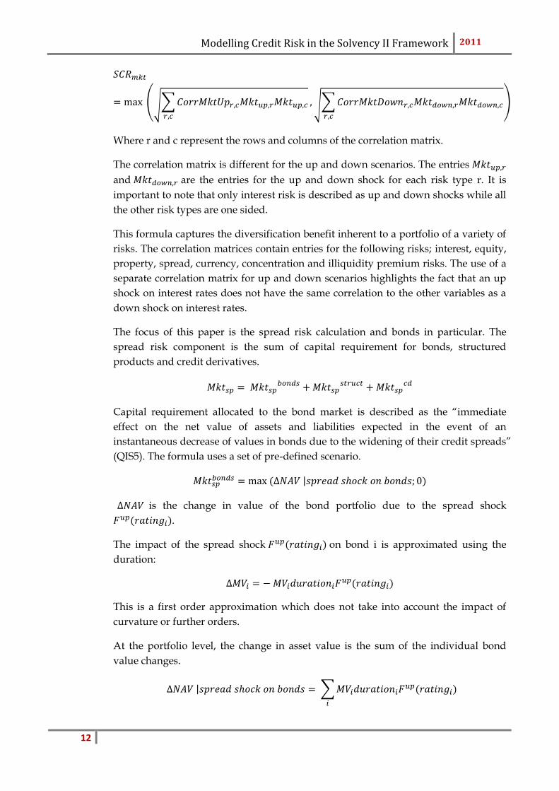
Where r and c represent the rows and columns of the correlation matrix.
The correlation matrix is different for the up and down scenarios. The entries
and are the entries for the up and down shock for each risk type r. It is
important to note that only interest risk is described as up and down shocks while all
the other risk types are one sided.
This formula captures the diversification benefit inherent to a portfolio of a variety of
risks. The correlation matrices contain entries for the following risks; interest, equity,
property, spread, currency, concentration and illiquidity premium risks. The use of a
separate correlation matrix for up and down scenarios highlights the fact that an up
shock on interest rates does not have the same correlation to the other variables as a
down shock on interest rates.
The focus of this paper is the spread risk calculation and bonds in particular. The
spread risk component is the sum of capital requirement for bonds, structured
products and credit derivatives.
Capital requirement allocated to the bond market is described as the “immediate
effect on the net value of assets and liabilities expected in the event of an
instantaneous decrease of values in bonds due to the widening of their credit spreads”
(QIS5). The formula uses a set of pre-defined scenario.
is the change in value of the bond portfolio due to the spread shock
.
The impact of the spread shock on bond i is approximated using the
duration:
This is a first order approximation which does not take into account the impact of
curvature or further orders.
At the portfolio level, the change in asset value is the sum of the individual bond
value changes.
Modelling Credit Risk in the Solvency II Framework 2011
13
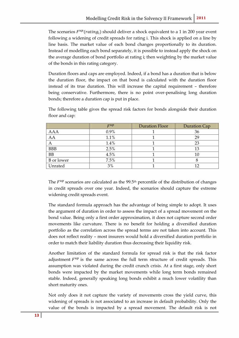
The scenarios should deliver a shock equivalent to a 1 in 200 year event
following a widening of credit spreads for rating i. This shock is applied on a line by
line basis. The market value of each bond changes proportionally to its duration.
Instead of modelling each bond separately, it is possible to instead apply the shock on
the average duration of bond portfolio at rating i; then weighting by the market value
of the bonds in this rating category.
Duration floors and caps are employed. Indeed, if a bond has a duration that is below
the duration floor, the impact on that bond is calculated with the duration floor
instead of its true duration. This will increase the capital requirement – therefore
being conservative. Furthermore, there is no point over-penalising long duration
bonds; therefore a duration cap is put in place.
The following table gives the spread risk factors for bonds alongside their duration
floor and cap:
Duration Floor Duration Cap
AAA 0.9% 1 36
AA 1.1% 1 29
A 1.4% 1 23
BBB 2.5% 1 13
BB 4.5% 1 10
B or lower 7.5% 1 8
Unrated 3% 1 12
The scenarios are calculated as the 99.5th percentile of the distribution of changes
in credit spreads over one year. Indeed, the scenarios should capture the extreme
widening credit spreads event.
The standard formula approach has the advantage of being simple to adopt. It uses
the argument of duration in order to assess the impact of a spread movement on the
bond value. Being only a first order approximation, it does not capture second order
movements like curvature. There is no benefit for holding a diversified duration
portfolio as the correlation across the spread terms are not taken into account. This
does not reflect reality – most insurers would hold a diversified duration portfolio in
order to match their liability duration thus decreasing their liquidity risk.
Another limitation of the standard formula for spread risk is that the risk factor
adjustment is the same across the full term structure of credit spreads. This
assumption was violated during the credit crunch crisis. At a first stage, only short
bonds were impacted by the market movements while long term bonds remained
stable. Indeed, generally speaking long bonds exhibit a much lower volatility than
short maturity ones.
Not only does it not capture the variety of movements cross the yield curve, this
widening of spreads is not associated to an increase in default probability. Only the
value of the bonds is impacted by a spread movement. The default risk is not
Modelling Credit Risk in the Solvency II Framework 2011
14
incorporated in the spread risk module while it is an important component of credit
risk. Default rates are not stable overtime – they should also be modelled
stochastically.
While taking into account the diversification benefit between risk categories, the QIS
5 formula does not take into account diversification benefit for holding a variety of
ratings. The evolution of the spreads amongst various ratings is not perfectly
correlated. Investors in short and long maturities do not have the same profile and
therefore, different events can have a different impact depending on the maturity and
rating. In that perspective, it is beneficial to use an internal model as it will highlight
the benefits of holding a diversified portfolio.
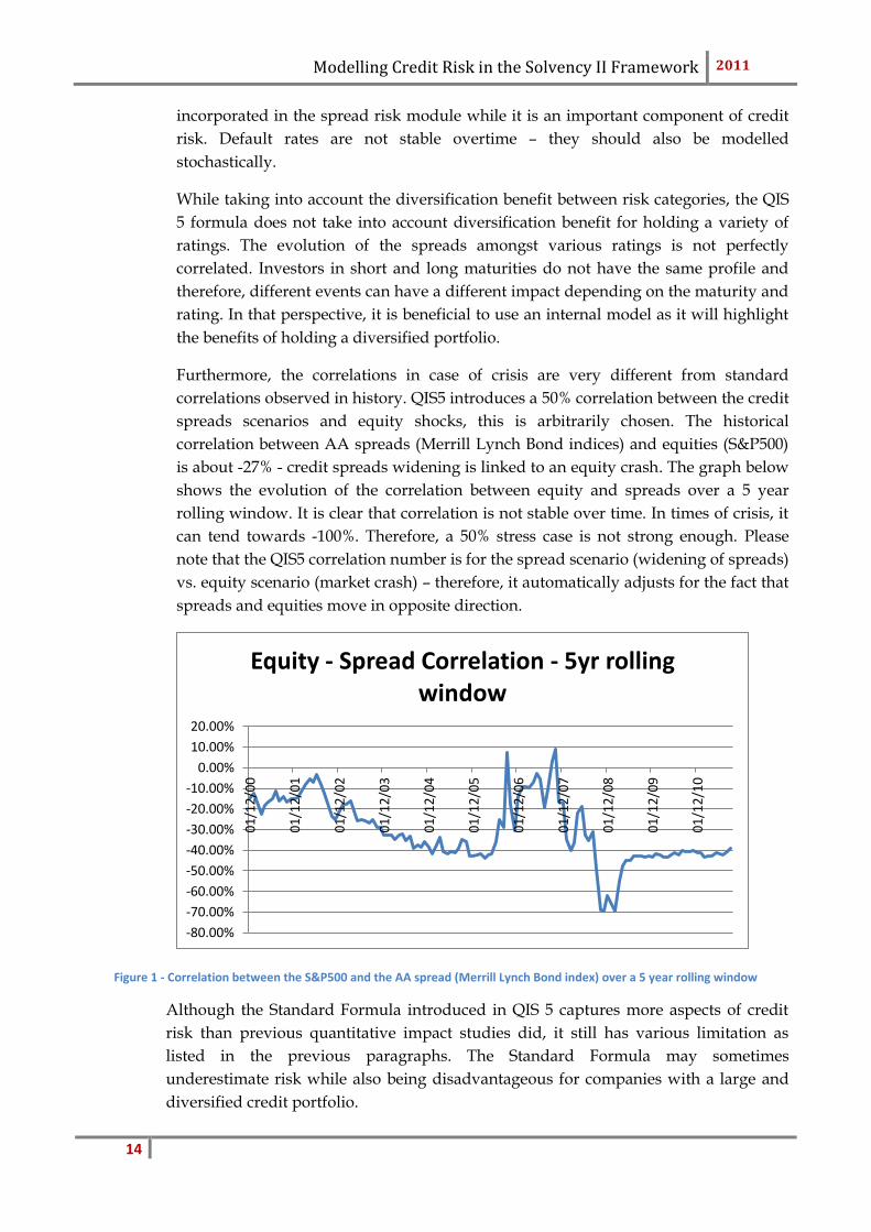
Furthermore, the correlations in case of crisis are very different from standard
correlations observed in history. QIS5 introduces a 50% correlation between the credit
spreads scenarios and equity shocks, this is arbitrarily chosen. The historical
correlation between AA spreads (Merrill Lynch Bond indices) and equities (S&P500)
is about -27% - credit spreads widening is linked to an equity crash. The graph below
shows the evolution of the correlation between equity and spreads over a 5 year
rolling window. It is clear that correlation is not stable over time. In times of crisis, it
can tend towards -100%. Therefore, a 50% stress case is not strong enough. Please
note that the QIS5 correlation number is for the spread scenario (widening of spreads)
vs. equity scenario (market crash) – therefore, it automatically adjusts for the fact that
spreads and equities move in opposite direction.
Figure 1 - Correlation between the S&P500 and the AA spread (Merrill Lynch Bond index) over a 5 year rolling window
Although the Standard Formula introduced in QIS 5 captures more aspects of credit
risk than previous quantitative impact studies did, it still has various limitation as
listed in the previous paragraphs. The Standard Formula may sometimes
underestimate risk while also being disadvantageous for companies with a large and
diversified credit portfolio.
-80.00%
-70.00%
-60.00%
-50.00%
-40.00%
-30.00%
-20.00%
-10.00%
0.00%
10.00%
20.00%
01
/12
/00
01
/12
/01
01
/12
/02
01
/12
/03
01
/12
/04
01
/12
/05
01
/12
/06
01
/12
/07
01
/12
/08
01
/12
/09
01
/12
/10
Equity - Spread Correlation - 5yr rolling window
Modelling Credit Risk in the Solvency II Framework 2011
15
Indeed, the report of the results of the QIS5 study shows that market risk is the biggest
risk hold by insurers. This is particularly true for life insurers where liabilities have
embedded options which require hedging techniques. Generally speaking, the biggest
risks are spread risk, equity risk and interest rate risk. The spread risk calculation was
strongly criticized as it was either producing too high or too low stresses. At the time
of writing this document, the final Solvency II recommendation is not published and
QIS5 will only serve as a base for the final regulation. In its current implementation, it
is apparent that large companies are more likely to opt for the (partial) internal model.
We will describe the internal model approach in the next section.
2.3 Internal or Partial Internal Model
As part of their Solvency II implementation, companies are allowed to use a (partial)
internal model instead of the Standard Formula. It permits a tailor made capital
management. It is therefore more interesting for bigger firms, although it comes at a
cost. Indeed, it is a more challenging approach; companies will need a great deal of
model development, parameterization and validation before their internal model is
approved. The results of QIS5 confirmed that most insurance companies are going
down the route of the internal model or partial internal model instead of using the
Standard Formula approach.
Instead of using a Standard Formula to calculate the capital requirement, a Monte
Carlo framework is used. It models all the risks faced by an insurance company in a
coherent way and calculates the profit and loss. The capital requirement is obtained
using a one year Value-at-Risk. It is set such that the insurance company holds
sufficient funds to absorb significant losses. The Value-at-Risk confidence level is
99.5 – meaning that ruin should not occur more than once every 200 years.
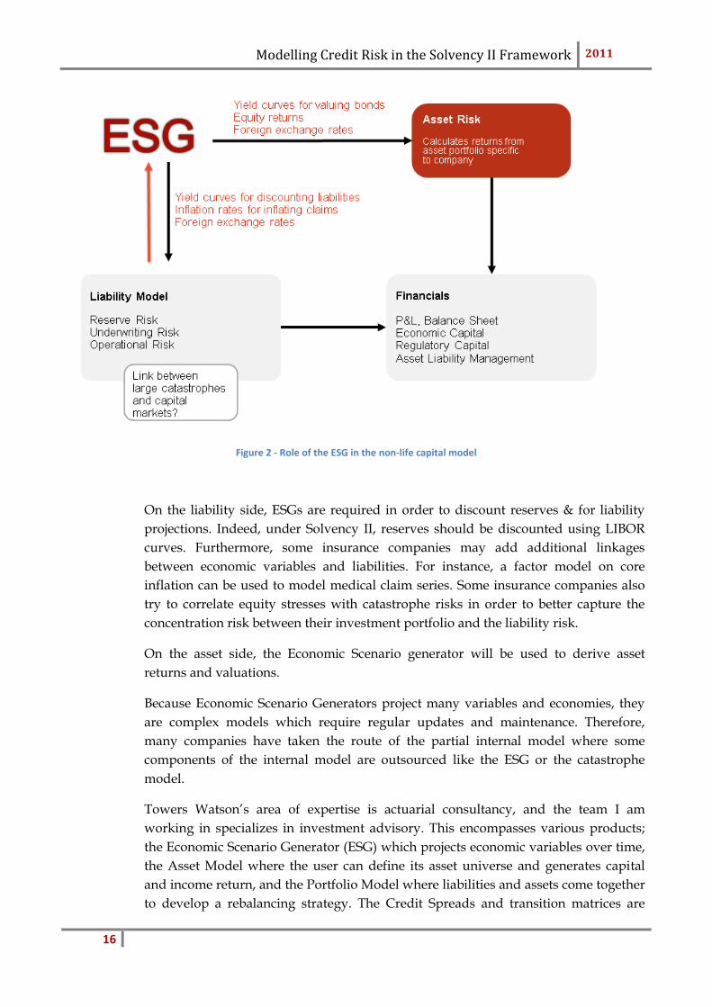
One of the key components of the capital model is the Economic Scenario Generator
(ESG). As mentioned previously, the aim of the internal model is to capture all the
risks faced by an insurance company – particularly modelling all the dependencies
between variables. Economic scenarios are projected using a Monte Carlo technique
and will feed both the liability and the asset side of the balance sheet. Figure 2
demonstrates the role of the ESG in the internal model of a typical non-life insurer.
Modelling Credit Risk in the Solvency II Framework 2011
16
Figure 2 - Role of the ESG in the non-life capital model
On the liability side, ESGs are required in order to discount reserves & for liability
projections. Indeed, under Solvency II, reserves should be discounted using LIBOR
curves. Furthermore, some insurance companies may add additional linkages
between economic variables and liabilities. For instance, a factor model on core
inflation can be used to model medical claim series. Some insurance companies also
try to correlate equity stresses with catastrophe risks in order to better capture the
concentration risk between their investment portfolio and the liability risk.
On the asset side, the Economic Scenario generator will be used to derive asset
returns and valuations.
Because Economic Scenario Generators project many variables and economies, they
are complex models which require regular updates and maintenance. Therefore,
many companies have taken the route of the partial internal model where some
components of the internal model are outsourced like the ESG or the catastrophe
model.
Towers Watson’s area of expertise is actuarial consultancy, and the team I am
working in specializes in investment advisory. This encompasses various products;
the Economic Scenario Generator (ESG) which projects economic variables over time,
the Asset Model where the user can define its asset universe and generates capital
and income return, and the Portfolio Model where liabilities and assets come together
to develop a rebalancing strategy. The Credit Spreads and transition matrices are

Modelling Credit Risk in the Solvency II Framework 2011
17
outputs from the ESG, while the credit risky bond returns are computed in the Asset
Model. The following section will describe in further detail the Towers Watson
Investment product suite.
Modelling Credit Risk in the Solvency II Framework 2011
18
3. The Investment Product Suite
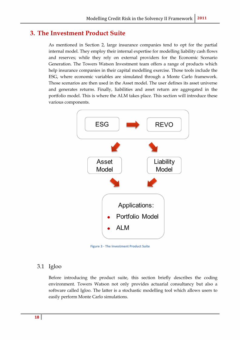
As mentioned in Section 2, large insurance companies tend to opt for the partial
internal model. They employ their internal expertise for modelling liability cash flows
and reserves; while they rely on external providers for the Economic Scenario
Generation. The Towers Watson Investment team offers a range of products which
help insurance companies in their capital modelling exercise. Those tools include the
ESG, where economic variables are simulated through a Monte Carlo framework.
Those scenarios are then used in the Asset model. The user defines its asset universe
and generates returns. Finally, liabilities and asset return are aggregated in the
portfolio model. This is where the ALM takes place. This section will introduce these
various components.
Figure 3 - The Investment Product Suite
3.1 Igloo
Before introducing the product suite, this section briefly describes the coding
environment. Towers Watson not only provides actuarial consultancy but also a
software called Igloo. The latter is a stochastic modelling tool which allows users to
easily perform Monte Carlo simulations.

Modelling Credit Risk in the Solvency II Framework 2011
19
The environment of this software is similar to Excel but with a visual component. One
can create base units which are then linked to each other. Variables are passed from
the output of one base unit to the input of another one. Calculations are performed in
each base unit. The software compiles the code automatically and handles the order
of calculations automatically and appropriately. As such it is a very easy
programming environment.
The draw of random numbers is generated in Igloo – generally using a Mersenne
Twister algorithm (although other algorithms are available).
The correlations between economic variables are applied by reordering simulations.
Again, this is handled automatically in the background.
A project in Igloo is like a spreadsheet in Excel. With the only difference that projects
can import results or data from other Igloo projects and then export values. It is
therefore possible to construct projects interacting with each other.
The investment products of Towers Watson are coded in Igloo. They are effectively
projects in Igloo whose outputs can be fed into other projects or exported to csv, excel
or databases. Given that most of Towers Watson’s clients build their capital model in
Igloo, the ESG & Asset model results are directly feeding the capital model. It is a
very efficient platform which can help reducing operational risk.
Figure 4 - Igloo
Modelling Credit Risk in the Solvency II Framework 2011
20
3.2 The ESG
There are two types of ESGs; risk neutral and real world. Risk Neutral ESGs are
typically used by banks for pricing derivatives. Indeed, by construction, risk neutral
ESGs are calibrated using market prices of derivatives today. The parameters are
inferred to match the pricing of such products at time 0. Such an ESG essentially
reflects the market’s view of the evolution of the world (e.g. implied volatility) but
contains limited historical analysis. Life insurers’ capital modelling uses such
scenarios in order to price embedded options in contracts. In effect, life insurance
liabilities require the use of replicating portfolios for their evaluation. Risk neutral
models are not appropriate for risk management and asset liability modelling.
Contrarily, a real world ESG focuses on the dynamics of economic variables in order
to generate realistic scenarios. Its calibration uses observed historical time series. It
produces coordinated scenarios which reflect the distributional properties of various
economic series. The main use of such series is risk management and as such the
models are not suitable for accurate forecasting or making short term trading
decisions. These models are also not suitable for derivative pricing purposes.
The Towers Watson Economic Scenario Generator consists of models for nominal
interest rate yield curves, real interest rate yield curves, LIBOR swap curves, equity
total (and price) return, dividend yields, price inflation (CPI), retail price index (RPI),
wage inflation, property total return, foreign exchange rates, gross domestic product,
federal funds rate (US only) and various indices (global hedge fund & HFRI sub
indices, commodities, global equities, emerging market equities, private equity, REIT
index, global high yield bonds, high yield emerging market). Each economic variable
has its own model – i.e. each variable follows a specific SDE. The dynamics of the
individual series is better captured. The number of years of projection, the number of
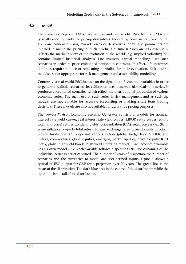
scenarios and the currencies to model are user-defined inputs. Figure 5 shows a
typical of ESG output for GBP for a projection over 20 years. The green line is the
mean of the distribution. The dark blue area is the centre of the distribution while the
light blue is the tail of the distribution.
Modelling Credit Risk in the Solvency II Framework 2011
21
Figure 5 - ESG Output Example
In order to produce the economic scenarios, each model is calibrated to historical data
as a first stage. The calibration process usually uses maximum likelihood or least
squared differences techniques. This can be challenging for processes where an
unobservable variable is required (e.g. stochastic volatility or regime switching). In
such instances, the use of a Kalman filter or of MCMC algorithms can be an
alternative. Our calibration does not focus on a particular time horizon; our aim is to
have realistic scenarios at the one year projection and at the long end. Depending on
the purpose of the ESG, users would need different lengths of projection. Indeed,
Solvency II capital modelling only requires one year projections. Nevertheless, in
order to simulate the run-off of liabilities, some insurance companies may require
ESG projections of more than 40 years. Therefore, our parameterization exercise
focuses on both short term and long term projections.
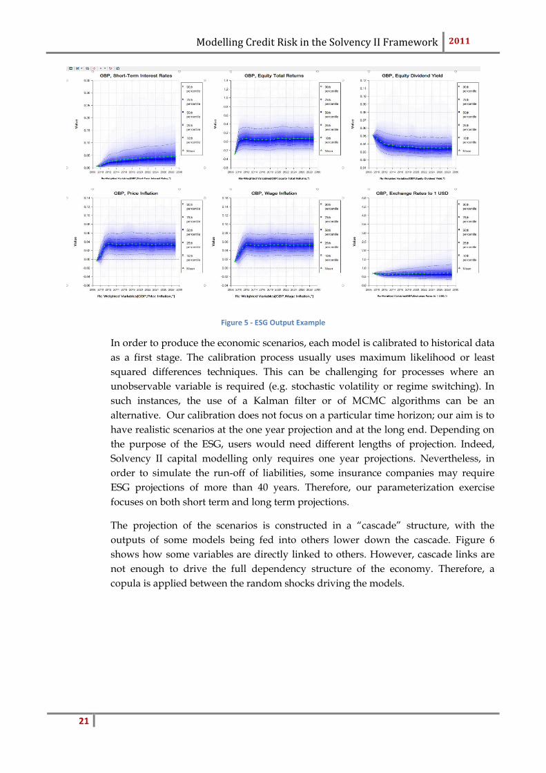
The projection of the scenarios is constructed in a “cascade” structure, with the
outputs of some models being fed into others lower down the cascade. Figure 6
shows how some variables are directly linked to others. However, cascade links are
not enough to drive the full dependency structure of the economy. Therefore, a
copula is applied between the random shocks driving the models.
Modelling Credit Risk in the Solvency II Framework 2011
22
Figure 6 - The ESG Cascade
In the calibration process, we obtain residuals from each model. We then study the
correlation between the residuals of each series and calibrate a grouped Student’s T-
copula. When generating this dependency structure, the ESG generates a set of
uniform variables which correlations and tail dependency satisfy the proprieties
imposed by the Grouped t-copula. Copulas allow the specification of the dependency
structure of a multivariate distribution. Because we model various economic variables
and economies, having the flexibility to specify a full correlation matrix between
every variable is necessary. Furthermore, it would be desirable to capture the
stronger tail dependency observed during a market crash. We opted for the Grouped
t-copula as it meets the two conditions. It allows for a different correlation between
different innovations but also allows for different degrees of “tail dependency”. Each
innovation is placed into a group (in the ESG, groups are currently made up from
economic variables from different currencies; for example, equity returns from
various currencies will be placed into one group, GDP forms another group etc.).
Innovations within a group have a Student’s t-copula dependency with a calibrated
number of degrees of freedom. The higher the number of degrees of freedom, the
closer to the Gaussian copula; the lower that number, the higher the tail correlation.
Between groups, the dependency structure is Gaussian; i.e. only the standard
correlation structure is applied.

Modelling Credit Risk in the Solvency II Framework 2011
23
Figure 7 - Example Tail Dependency between Equity Markets
In the ESG projection, the first step is to generate the dependency structure. We
simulate the normal draws that are linked via the copula. These innovations are then
fed into the individual models and each economic variable is projected according to
its own model/equation. By construction, the variables are correlated through both
the copula and the cascade structure.
Figure 7 shows the correlation between two equity series (GBP and USD) as a heat
map. It is clear that thanks to the Grouped t-copula, the tail dependency is enhanced.
The Towers Watson ESG only generates economic variables; it does not generate asset
returns such as bond returns. Some ESG providers have decided to calibrate bond
series to existing bond indices. Users would then have to rely on this subset of indices
to replicate their portfolio. In our opinion, this isn’t granular and flexible enough.
This is why the ESG is calibrated to generic yield curves and spreads term structures.
The Asset model is then used to generate the bond returns and other asset classes.
Modelling Credit Risk in the Solvency II Framework 2011
24
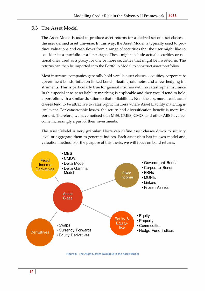
3.3 The Asset Model
The Asset Model is used to produce asset returns for a desired set of asset classes –
the user defined asset universe. In this way, the Asset Model is typically used to pro-
duce valuations and cash flows from a range of securities that the user might like to
consider in a portfolio at a later stage. These might include actual securities or no-
tional ones used as a proxy for one or more securities that might be invested in. The
returns can then be imported into the Portfolio Model to construct asset portfolios.
Most insurance companies generally hold vanilla asset classes – equities, corporate &
government bonds, inflation linked bonds, floating rate notes and a few hedging in-
struments. This is particularly true for general insurers with no catastrophe insurance.
In this special case, asset liability matching is applicable and they would tend to hold
a portfolio with a similar duration to that of liabilities. Nonetheless, more exotic asset
classes tend to be attractive to catastrophic insurers where Asset Liability matching is
irrelevant. For catastrophic losses, the return and diversification benefit is more im-
portant. Therefore, we have noticed that MBS, CMBS, CMOs and other ABS have be-
come increasingly a part of their investments.
The Asset Model is very granular. Users can define asset classes down to security
level or aggregate them to generate indices. Each asset class has its own model and
valuation method. For the purpose of this thesis, we will focus on bond returns.
Figure 8 - The Asset Classes Available in the Asset Model
Modelling Credit Risk in the Solvency II Framework 2011
25
For bond returns, the asset model values the assets using a discounted cash flow
method. Cashflows are calculated by the exact date and then discounted using the
yield curves of the ESG. The aim of the model is to generate asset indices. The user
can specify rebalancing rules; “hold”, “reset” or “hold & reset”. Where a subclass is
set to “hold”, the securities will be held until redemption – such that the group is ef-
fectively run off until nothing remains. Where the subclass is set to “reset”, it will re-
balance to the original profile by selling the securities at the end of the period and us-
ing the proceeds to buy new securities with the original parameters. Finally, where
the subclass is set to “hold & reset”, the security will be held until redemption. The
principal redeemed is used to rebalance the matured security to its original profile.
This last method is a combination of the two previous methods. The flexibility in re-
balancing methods is very interesting to insurance companies which look at asset li-
ability modelling and try to keep the duration of their portfolio constant.
For other asset classes that are more complex, the discounted cash flow method is not
applicable. For instance, a proxy model is used to compute ABS returns. The user can
input the delta and gamma to some interest rates.
Derivatives are not available in the asset model as one would need a risk neutral ESG
in order to value these. It is nonetheless possible to use derivatives as hedging in-
struments where only the cash flows are modelled but the asset is not valued and
cannot be traded.
Another very important feature available in the asset model is the risk split. Returns
are split by capital and income return as well as by risk category: Equity risk, spread
risk, FX risk, interest rate risk. This is one of the Solvency II requirements; insurance
companies should be able to identify the exposure to those individual risks.
Please note that the Solvency II credit risk definition does not contain elements of
market risk but only concerns reinsurance and premium debtors default risk – it is
therefore a counterparty risk which has to be modelled separately from the main
market risk exposure. Spread risk on the other hand is the aggregation of bond de-
faults, migrations and spread movements – thus only focusing on market risk. Equity,
FX, and interest rate risk are all part of the market risks exposure.
3.4 The Portfolio Model and ALM tools
Once the asset returns have been generated in the asset model, the user specifies its
investments in the individual asset classes in the portfolio model. Furthermore,
rebalancing rules are included and import liability cash flows imported. The portfolio
model will automatically sell and buy assets based on the liability outflows and
reinvestment rules.
Modelling Credit Risk in the Solvency II Framework 2011
26
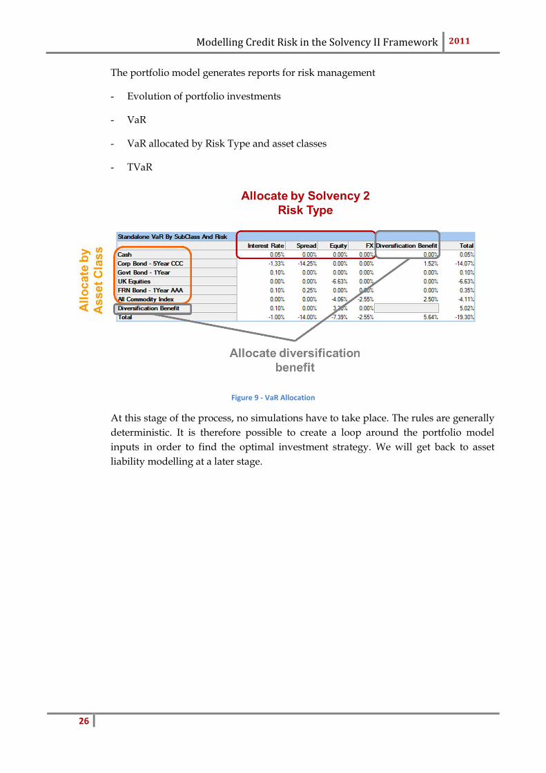
The portfolio model generates reports for risk management
- Evolution of portfolio investments
- VaR
- VaR allocated by Risk Type and asset classes
- TVaR
Figure 9 - VaR Allocation
At this stage of the process, no simulations have to take place. The rules are generally
deterministic. It is therefore possible to create a loop around the portfolio model
inputs in order to find the optimal investment strategy. We will get back to asset
liability modelling at a later stage.
Modelling Credit Risk in the Solvency II Framework 2011
27
4. Introduction to Credit Risk
In this section we will review the credit modelling approaches available in the
literature. We will start with the general measures of credit risk – transition matrices
and credit spreads. And then we will move the idiosyncratic types of models.
4.1 Probabilities of Default and Credit Spreads
In the bond market, there are two types of investment; government bonds and
corporate bonds. Government bonds are assumed to be risk free (with some
limitations, please refer to section 5.2). The risk free yield curve can be backed out
from government bond prices. Corporate bonds, on the other hand, can default; this
makes them risky investments. Investors do not wish to bear the risk unless it is
compensated by a higher return. As for government bonds, assuming a company has
emitted bonds with various maturities, a risky yield curve can be inferred from the
bonds available in the market. The spread between the risky yield curve and the risk
free yield curve is called the credit spread.
It is frequent to assume that bond prices vary with interest rates (risk free yield curve)
and default probability of a company. Thus, credit spreads should directly reflect the
chances of a company defaulting. It is worth noting that this is limited to the theory.
Indeed, during the credit crisis, credit spreads were sky rocketing without a direct
linkage to a similar increase in probabilities of default. Fear in the market and lack of
liquidity are also important contributors to credit spread movements.
4.2 Ratings, Scores & Transition Matrices
In order to assess the credit quality of a firm, various approaches are used in the
market. Depending on the time horizon of interest, one would use the “at-the-point-
in-time” methods or “through the cycle” methods.
The first type of method assesses the credit quality of a firm over the coming months.
Such approaches use quantitative methods or structural models looking at the
debt/equity ratios.
The second type of method is less volatile as its aim is to capture the creditworthiness
over a long time horizon. Ratings are more stable over time. The methodology
includes the whole business cycle - peaks and droughts of the economy. Generally,
transition matrices reflect through-the-cycle probabilities.
Rating agencies affect a rating to most issued bonds. These should reflect the issuing
companies’ creditworthiness. The existing three main rating agencies use their own
Modelling Credit Risk in the Solvency II Framework 2011
28
method to assess the probability of default of companies. Ratings are the main
indicator of spread level and are the easiest way to group issuers in a model.
Furthermore, rating agencies publish rating transition matrices which give the
probability of migration from one rating to another over the course of one year. These
matrices are published on a yearly basis. Our analysis is based on the S&P Annual
Global Corporate Default Study and Rating Transitions and contains both an average
transition matrix calculated using data from 1981 but also the current year’s transition
matrix.
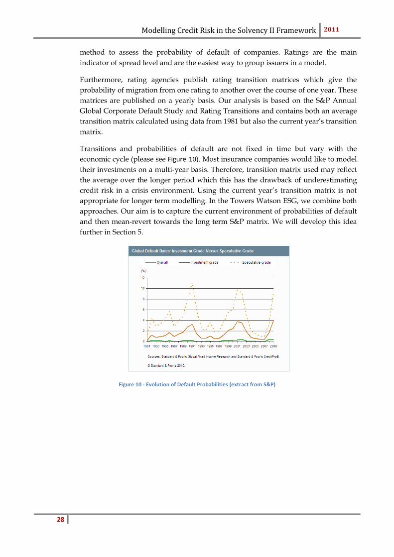
Transitions and probabilities of default are not fixed in time but vary with the
economic cycle (please see Figure 10). Most insurance companies would like to model
their investments on a multi-year basis. Therefore, transition matrix used may reflect
the average over the longer period which this has the drawback of underestimating
credit risk in a crisis environment. Using the current year’s transition matrix is not
appropriate for longer term modelling. In the Towers Watson ESG, we combine both
approaches. Our aim is to capture the current environment of probabilities of default
and then mean-revert towards the long term S&P matrix. We will develop this idea
further in Section 5.
Figure 10 - Evolution of Default Probabilities (extract from S&P)

Modelling Credit Risk in the Solvency II Framework 2011
29
4.3 Merton Model
In essence, credit spreads are meant to reflect the probability of default of a company.
It is thus sensible to look at the capital structure. This is the approach introduced by
Merton. This model falls into the idiosyncratic category of models as it analyses
individual companies in isolation.
The Merton model originated from Black and Scholes who suggested that their
methodology could be extended to corporate security pricing. Indeed, a firms with
value V is financed through equity (S) and discount bonds (value P and maturity T).
The debt principal is K. The value of the firm at time t is
The model then assumes that the value of the firm follows a Geometric Brownian
Motion. Default is triggered by the event . This relies on one major assumption;
bond holders cannot force the firm to go bankrupt before the maturity of the debt.
In the event of default, bondholders have priority over equity holders and receive .
Otherwise, they receive the principal of the debt, K. This payoff can be seen as the
payoff of a riskless bond minus a put option on the value of the firm. Indeed,
.
Shareholders receive nothing in the event of default but would profit from the upside
if the firm remains solvent. Their payoff is a call option on the value of the firm with a
strike K:
According to the Black-Scholes formula for option pricing, the equity value is
obtained immediately:
Where r is the risk free rate, and the volatility of the firm’s value.
Although this model sounds appealing as it brings a lot of insight on the relationship
between the value of a firm and its securities, it relies on many strong assumptions,
E.g.:
- the capital structure is very simplistic
Modelling Credit Risk in the Solvency II Framework 2011
30
- it is assumed that one can observe the value of the firm easily and that it follows a
GBM
- riskless interest rates are constant
- there is no debt renegotiation
- default occurs at the debt maturity only
Many extensions to this approach have been published. One of which was to extract
probability of default from equity prices. This is the basis of the KMV credit method.
Once the structure of the debt is known, it is possible to back out the distance to
default k. N(-k) would give the default probability (with N the cumulative normal
distribution). KMV have extended this idea.
The problem of this method is that the probability of default obtained here is a point
in time measure. Ratings on the other hand are through-the-cycle assessments of
creditworthiness. When one is looking at tactical asset allocation and needs
information to price individual issues, such a method becomes attractive.
Nevertheless, a lot of information is required from the debt structure and it relies on a
significant number of assumptions. In the context of risk management, this method is
not appropriate.
We will now introduce another type of idiosyncratic models – the intensity based
models.
4.4 Credit Intensity Models – Reduced-form models
Intensity models (also called reduced-form models) consider the default of a
company to be an exterior event which hits the company by accident. The probability
of the default event is extracted from bond prices.
The default time is modelled as the first jump of a Poisson process. The probability of
a jumping in the next time interval dt is
is called the intensity or hazard rate, it is assumed to be strictly positive.
Depending on the specification of the model, the intensity rate is deterministic or
stochastic (often modeled as a Cox Ingersoll Ross process).
It then flows that the probability of the bond surviving past maturity (survival
probability at t) is

Modelling Credit Risk in the Solvency II Framework 2011
31
This is very similar to the price of a zero coupon bond in an interest rate model where
the short rate is replaced by the hazard rate.
Furthermore, one can then compute the price of a risky zero coupon bond:
From this notation, it becomes clear that the hazard rate is the credit spread.
One of the limitations of this model is that the hazard rate is modelled independently
of the other sources of randomness. Furthermore, the credit spreads of individual
companies are modelled stochastically but not in an integrated manner.
In the context of a bond portfolio, one isn’t interested in the individual riskiness of the
issuers - the so-called idiosyncratic risk. Instead, it is the systematic nature of the risk
that should be focused on.
Modelling Credit Risk in the Solvency II Framework 2011
32
5. The JLT framework and extensions
In the previous section, we have introduced the link between probabilities of default
and credit spreads. Furthermore, we have looked at transition matrices and their
information content with regards to bonds’ riskiness. The two models presented in
the previous section do not take advantage of rating information. These two models
are ideal when a defined security should be priced – indeed, the focus should then be
on idiosyncratic risk. When it comes to risk management, systemic risk should be
looked at and therefore a different model is required.
5.1 The JLT framework & alternatives
The Jarrow, Lando and Turnbull model focuses on the link between probabilities of
default and credit spreads. Based on a transition matrix, credit spreads are inferred
directly. This assumes that corporate bond prices are only driven by rating and
maturity.
The model stems from the correspondence between the risk neutral probability of
default and the bond price. Indeed, credit risky bond prices can be linked to the
survival probability. If the bond survives up to maturity , the owner will
receive principal repayment. But if the bond defaults before maturity , the
owner receives the recovery rate Therefore, the price of a bond at time t with rating
i and maturity T is as follows:
Where Q is the risk neutral probability measure, is the risk free rate, is the
recovery rate, the time of default.
This translates into the following decomposition between risk free bond prices and
survival probability.
We denote by B(t,T) the price of a risk free bond at time t and maturity (T-t), is
the probability of going from rating i to default between t and T.
Please note that the probability of default q is the risk neutral probability over the
periods T-t. Indeed, K is the default state – assuming we have K-1 ratings. This is a
discrete probability. It is important to note that the transition matrices produced by
rating agencies are always provided with a time horizon – generally one year. Indeed,
the probabilities change depending on the time horizon. A common assumption is
that probabilities of migrations and default follow a Markov chain process. Indeed,
Modelling Credit Risk in the Solvency II Framework 2011
33
the yearly transition matrix can be compounded in order to obtain the transition
probabilities over 2 years.
At this stage, it can be useful to mention continuous and discrete transition matrices.
The transition matrices provided by rating agencies express discrete probabilities.
When looking at stochastic processes and bond prices, it is much easier to work in the
continuous world. Therefore, generator matrices are used instead. The discrete (Q)
and continuous matrices ( are related by the following relationship:
The sum of rows in a discrete matrix is equal to 1. The sum of rows of the generator
matrix is equal to 0. Therefore, Λ is of the form:
From the formula linking the price of a risky bond and the probability of default, we
can get a relationship between credit spreads and probabilities of default. Indeed, the
price of a risk free bond is
Where f is the instantaneous forward rate.
The price of a risky bond is:
Where defines the instantaneous forward credit spread.
This means that there is a direct correspondence between default probabilities and
forward credit spreads:
Here, we have q the probability of default between t and T; is the instantaneous
forward spread.
We will use this relationship throughout the paper. Indeed, the proposed model relies
on the correspondence between transition matrices and credit spreads.
The probabilities of migrations and defaults presented in the formulas above are risk
neutral probabilities. Indeed, credit spreads are risk neutral instruments. The
transition matrix obtained from rating agencies is real world as it is calculated from
observed default and migrations over time. The JLT model differentiates itself from
the previous models by introducing a risk premium to move from real world to risk
neutral probabilities. The relationship between spreads and probabilities of default
Modelling Credit Risk in the Solvency II Framework 2011
34
does not work with real world probabilities and couldn’t be exploited. In order to
match bond prices observable in the market, the use of a risk premium is required.
JLT introduce the following specification:
This form of risk premium can generate negative spreads. It is possible to address this
issue by specifying another form of risk premium
Nevertheless, its main disadvantage is that it does not allow for stochastic spread
variation. Indeed, the risk premium used in the model is deterministic and thus the
spreads movements are non-existent.
Many papers mention extensions of the JLT model in order to project stochastic
spreads linked to transition matrices. Towers Watson’s previous approach was to
apply a stochastic multiplicative adjustment to the generator matrix. A Cox Ingersol
Ross process was used as a multiplicative factor to the transition matrix. This means
that there exists a closed-form formula for bond prices. The process being positive
ensured transition rates remained positive – and so were spreads. Furthermore, we
would force the process to revert towards 1; therefore, this forced the transition rates
to revert towards the S&P matrix over the long run.
Please note that in order to force the process to revert to 1, we would set the long
term mean b to 1. a is the speed of mean reversion and sigma the volatility of the
process.
Although this model has the advantage of being simple and parsimonious, it has a
few drawbacks. Firstly, only very few parameters drive the evolution of the model;
the volatility, mean reversion rate and risk premium. The mean reversion level is
fixed to one in order to ensure the matrix reverts towards the S&P matrix. This means
that only three parameters can be changed to fit the historical spreads for all ratings.
It is impossible to match the starting term structure of credit spreads for all ratings
given the limited number of degrees of freedom. Instead, only one rating can be used
in the calibration process.
Furthermore, there is considerable heterogeneity between rating classes for corporate
bonds. All ratings are not impacted by the same events or news, their evolution can
diverge. For instance, at the beginning of the credit crunch crisis, mostly non-
investment grade bonds were affected before it spread to investment grade. Given
that it is only a one factor model; the spreads by ratings obtained in the projection are
fully correlated. This is not realistic.
Modelling Credit Risk in the Solvency II Framework 2011
35
Thirdly, the scalar transition intensity modification does not fully represent the true
dynamics of the ratings migration process. For example, when the credit intensity
parameter is high, the model will tend to produce more defaults, but also more
upgrades. In reality, an economic downturn would tend to produce more
downgrades and defaults and fewer upgrades.
Finally, the distribution of this credit model does not capture the tail distribution
correctly. Even though the volatility of the CIR process is calibrated to historical
spreads, the distribution cannot replicate spreads levels as observed during the credit
crunch.
We will compare the results of this model against the Arvanitis Gregory and Laurent
extension – the current approach – in the results section.
5.2 The Arvanitis Gregory and Laurent Extension
Arvanitis, Gregory and Laurent have extended the JLT framework in order to capture
stochastic credit spreads as well as stochastic transition & default probabilities.
In our model, we use the S&P transition matrix but any other rating agencies’ matrix
could be used instead. Bonds are grouped by categories of creditworthiness, from
AAA to CCC rating.
The process by which issuers migrate between credit categories denoted i=1,…,K-1
and the default state K, is modelled as a continuous time Markov process with gen-
erator matrix .
With .
The generator matrix is related to the transition probability matrix through the fol-
lowing relationships:
Modelling Credit Risk in the Solvency II Framework 2011
36
The latter equation relies on one assumption – the matrices need to be commu-
tive. Indeed, we only have exp(A+B) = exp(A) + exp(B) when the square matrices A
and B commute (AB = BA).
The generator matrix is then decomposed into eigenvalues and eigenvectors. We have
as many eigenvalues as the number of credit ratings, i.e. eight (incl. the default state),
and eight eigenvectors with eight elements each. The spectral decomposition of the
generator is
Where represent the (right) eigenvectors and the eigenvalues of
respectively.
The Arvanitis Gregory and Laurent paper states that it is empirically observed that
the eigenvectors are stable over time, therefore we assume these to be constant. This
is critical in order to ensure that the commute - therefore validating the assump-
tion made earlier in the document. Nevertheless, this assumption is very restrictive.
As mentioned in Lando, it means that the family of generators has a common set of
eigenvectors regardless of how the process for the state variables evolves.
Given that the eigenvectors are assumed constant, they are calculated directly from
the historic S&P transition matrix. On the other hand, the eigenvalues are modelled
stochastically.
A closed form formula links the risk neutral probability of default by rating and the
term structure of credit spreads.
Where is the recovery rate and the probability of default between t and T
for rating i.
The probability of default is linked to the process followed by the eigenvalues as de-
scribed by the following formula:
Modelling Credit Risk in the Solvency II Framework 2011
37
Where is the conditional expectation given all information available up to ,
is the (i,j)th element of , the (i,j)th element of . The are the eigenvalues by rat-
ing.
The formula above is quite intuitive. It is apparent that the probability of default for
rating i depends on the sum of probabilities to move from rating i to rating j and then
from rating j to default (K).
Please note that the sum does not include j = K. Indeed, the result stems from the fol-
lowing relationship:
State K is an absorbing state - = 0 and the last row of is equal to (0,0…,0,1). It
can be demonstrated that it is the unique invariant of the Markov chain.
Instead of modelling each eigenvalue individually which would be inefficient, the ei-
genvalues are driven by a three-factor mean-reverting Ornstein-Uhlenbeck (OU)
model. A Principal Components Analysis (PCA) is applied on the time series of cen-
tred and normalised eigenvalues in order to isolate the first three components.
We define the centred reduced eigenvalues by
where is the mean of the jth historical eigenvalue and the standard deviation of
the historical data set.
The first three factors obtained from the PCA analysis explain about 98% of the total
correlation for most economies. In our model, we assume that those three factors fol-
low an Ornstein-Uhlenbeck process as per the equation below:
With
,
,
and
(Please note that the are independent from each other)
We force the mean reversion level to be zero as the eigenvalues have already been
centered before applying the PCA. Furthermore, the three processes are independent
because the three factors are orthogonal by construction.
The following parameters drive the OU process:

Modelling Credit Risk in the Solvency II Framework 2011
38
- The speed of mean reversion measures how fast the process reverts towards
its equilibrium levels. This parameter is common for all three factors (see the
section on calibration for reasoning behind this assumption);
- The volatility coefficients measure the degree of volatility (amplitude of
fluctuation) of the eigenvalues about their equilibrium levels. There are three
volatility coefficients for each factor applying.
Furthermore, the following parameters are required in order to recover the projected
eigenvalues:
- The principal component (PCA) coefficients are obtained from the PCA.
These are summarized in a three by eight matrix (factors times number of rat-
ings).
- The mean ( and standard deviation ( of the historical eigenvalues for
each credit rating: these are necessary, since in this approach we model cen-
tred eigenvalues which we further scale by their standard deviations;
The
can be recovered from the three processes using the following
relationship:
where
is the principal components matrix (obtained
through the PCA)
Therefore the eigenvalues can be expressed as a function of the Ornstein-Uhlenbeck
process:
The use of a three factor Ornstein-Uhlenbeck enables us to obtain a closed form solu-
tion for default probabilities:
The integral of the eigenvalues are normally distributed. It is
Modelling Credit Risk in the Solvency II Framework 2011
39
We can therefore apply the moment generating function of a normal variable which
gives us:
Using the closed form solution of the Ornstein-Uhlenbeck process, it can be easily
demonstrated that:
In the formulas above we note ttm as the time to maturity (T-t), as the historical
mean of the eigenvalues, are the simulated eigenvalues, are the historical stan-
dard deviations of the eigenvalues, is the standard deviation of the OU process k.
Instead of applying a discretization scheme, we can use those closed-form formulas at
the simulation stage.
The use of a three-factor Ornstein-Uhlenbeck ensures that the ratings are not fully
correlated. This addresses some of the limitations of the credit model introduced in
5.1.
5.3 Challenges for risk management, introduction of risk premiums
When modelling a bond portfolio, it is not only required to model credit spreads but
also to capture migrations and defaults. This has been introduced in section 3.3 – the
asset model. So far, we have concentrated on credit spreads. These are risk neutral
measures of credit risk. The model introduced by Arvanitis, Gregory and Laurent
described in 5.2 produces risk neutral migration intensities which are used to
generate the term structure of credit spreads. For risk management purposes, we will
Modelling Credit Risk in the Solvency II Framework 2011
40
require the real world transition probabilities are driving transitions. For that matter,
the model needs to be extended to the real world.
The S&P transition matrix is based on the average default and transitions observed
between 1981 and 2010. We assume this to be the long term level of migrations and
defaults which will ensure the real world model reverting towards this target. The
starting point is calibrated to the current level of credit spreads. This implies that be-
fore reaching the equilibrium level, the model produces periods of high default rates,
but also benign periods of low default rates.
To achieve this, a risk premium adjustment was added to the OU process in order to
move to the real world probability measure. This gave good results but some
information was lost through the PCA and the long term level was not in line with
the S&P matrix. Instead, we now use a risk premium adjustment for each eigenvalue.
Indeed, by construction of the OU process, the risk neutral eigenvalues revert
towards their historical average. It is therefore easy to make the real world
eigenvalues converge towards the S&P historical eigenvalues.
In order to move from the risk neutral to the real world transition matrix, a risk pre-
mium is applied to the eigenvalues.
With the risk premium factor for the ith eigenvalue.
This risk premium is obtained through an optimisation algorithm. Its goal is to obtain
a long term real world transition matrix as close as possible to the S&P transition ma-
trix. Furthermore, one of the constraints of this optimiser is to ensure the starting real
world matrix captures the order of riskiness (the probability of default of a AAA
bond is lower than that of a AA bond).
The real world transition matrix is computed with the real world eigenvalues:
An alternative specification for the risk premium would be to include it as part of the
Ornstein Uhlenbeck process. This would represent an appropriate change of measure
where the martingale property is respected. There would be only 3 risk premium pa-
rameters – one by OU process. This was our first approach but it became apparent
that having only 3 degrees of freedom was not enough to achieve a good fit of the his-
torical transition matrix. Indeed, the average of the simulations at the long term hori-
zon was not perfectly aligned with the S&P matrix used as reference. This led us to

Modelling Credit Risk in the Solvency II Framework 2011
41
use this risk premium adjustment instead. The proof that it is an appropriate change
of measure will be investigated at a later stage.
Another challenge of modelling transition matrices from credit spreads is the high
volatility. There are many components of risk which form credit spreads, the major
one being the default & migration probability. In addition to this, there is liquidity
risk and idiosyncratic risk. Historically, the transition rates and default probabilities
exhibit less volatility over time than credit spreads imply. The current model as it
stands is calibrated to credit spreads, thus reflecting their volatility. The transition
matrix output is therefore too volatile. For that reason, before moving to the real
world, a default adjustment was introduced to reduce the volatility of default rates.
This factor is calculated to capture the extremes of the level of defaults as seen in his-
tory. It is the same for all economies and fixed at 0.4. In order to reduce the volatility
uniformly, it is applied to the Ornstein-Uhlenbeck process; the vector .
The transition matrix projections use similar techniques as the one applied for credit
spreads. The same stochastic process drives the credit spreads evolution and the tran-
sition matrix. Eigenvalues are only modified by the risk premium adjustments in or-
der to obtain a real world matrix.
We use the following relationship (described in the previous section).
As per the credit spreads formula, we have:
The only difference between risk neutral and real world is the mean term via the
presence of the risk premium adjustment.
In the formulas above we note ttm as the time to maturity (T-t), as the historical
mean of the eigenvalues, are the simulated eigenvalues, are the historical stan-
dard deviations of the eigenvalues, is the standard deviation of the OU process k.
Modelling Credit Risk in the Solvency II Framework 2011
42
The time to maturity used for the calculation of the transition matrix is one year as it
is common practice to look at the one year transition matrix. When it is required to
model bond returns on a quarterly basis, a quarterly transition matrix is required. To
do so, we use the formula described previously and integrate the eigenvalues over
one quarter – therefore setting ttm to be equal to 3 months.
This model can sometimes give negative probabilities of default and negative
spreads. This is further detailed in the section limitations. Nevertheless, it is impor-
tant to note that at the projection stage, we force the probabilities of default to be
positive. We thus use the following relationship:
The transition rates no longer sum to one and consequently need to be rescaled.
So far, we have focused on the model itself and how to obtain credit spreads and
transition probabilities in an integrated way. Nevertheless, the biggest challenge
posed by this model is its calibration. The following section will examine the process
followed.
5.4 Calibration
Transition and default probabilities are directly observable using statistics of compa-
nies and bonds. Credit spreads on the other hand are inferred from traded products
on the markets and thus contain risk premium adjustments. Because of this risk pre-
mium, credit spreads cannot be obtained directly from real world or observed transi-
tion matrices; an adjustment needs to be made to compensate for it. As explained in
the previous section, we need to evolve two transition matrices in parallel, one which
reflects the probabilities of bonds defaulting (the real world transition matrix) and
one containing the embedded risk premium adjustments from which bond prices and
credit spreads can be inferred (the risk neutral transition matrix). Because of this, our
calibration process has to be structured in three phases. The first one computes the ei-
genvalues from the history of credit spreads. At the second stage we obtain the pa-
rameters of the Ornstein Uhlenbeck. Finally we calculate the risk premium adjust-
ment.
Our calibration process uses the Merrill Lynch bond indices – particularly the option
adjusted spread data. Daily data is available from Bloomberg for many countries and
is split by rating and duration. However, the full term structure of bonds is not avail-
able from that index. We generally obtain a short maturity (around 2 years) and a
longer one (around 10-15 years) for each rating category and country. As part of our
data set, we also have the average duration of the index at each time step. The indices
Modelling Credit Risk in the Solvency II Framework 2011
43
are formed from a variety of bonds – the pool is regularly updated in order to keep
duration around a constant level. The data set starts around 2000.
Another important element of the calibration is the S&P transition matrix. We use the
one year transition and default matrix calculated using data from 1981. From that we
calculate the generator matrix (we calculate the eigenvalues and eigenvectors and ap-
ply a logarithm to the eigenvalues). As explained in the specification of the model, we
assume that the eigenvectors are constant over time. They will be used all along in the
calibration and projection.
We can then start with the first step of the calibration process – calculating the time
series of eigenvalues from the credit spreads. Indeed, we do not have history of tran-
sition rates from the data set. We only have credit spreads. In order to obtain the pa-
rameters of the Ornstein Uhlenbeck, we need the history of eigenvalues. These should
not be seen as parameters but rather latent variables.
Using the historical spread time series for each rating category at various maturities,
we determine the series in the risk neutral framework. To do so, we use the rela-
tionship between the spread of a specified rating and the eigenvalues of the
tor .
The formula above requires the parameters of the Ornstein Uhlenbeck and the prin-
cipal components – which will only be estimated at a later stage once we have the his-
tory of eigenvalues. We will explain later how we go around this problem.
We perform an optimisation minimising the difference between the historical spreads
and the theoretical ones. The theoretical spread is a function of the parameters of the
Ornstein-Uhlenbeck process and the principal components.
Therefore the optimization problem is expressed as:
With
As the data window can be as long as 13 years on a monthly basis, there are up to
1094 unknowns and finding one solution is not possible. It is worth nothing that the
spreads cannot be expressed as a function of , only. Indeed the principal

Modelling Credit Risk in the Solvency II Framework 2011
44
components are also prevalent in the formula. Because the principal components
are retrieved from the PCA performed on the very same eigenvalues that are being
estimated here, they are unknown at this stage. This goes into a full loop.
For this reason, we need to make some simplifications. Under certain assumptions,
the term involving the principal components in the spread formula can be ignored.
Indeed, in the spread formula, the only term which includes the principal compo-
nents is
If , it can be approximated by
In our data set, the short term bonds forming the indices used in the calibration have
an average maturity between 1Y and 3Y and it can be noted that , therefore
we assume that the term in the spread formula can be neglected during the calibra-
tion process.
From this simplification we obtain the following formula for the theoretical spread
(please note that at this stage, we assume that .) :
With the probability of default between t and T for rating i.
With the (i,j)th element of , the (i,j) element of and the long term
mean. In the calibration process these values are approximated by
Using the previous approximation, the spread formula is not a function of PC and
anymore. Furthermore, we split the optimisation problem into solvable sub problems
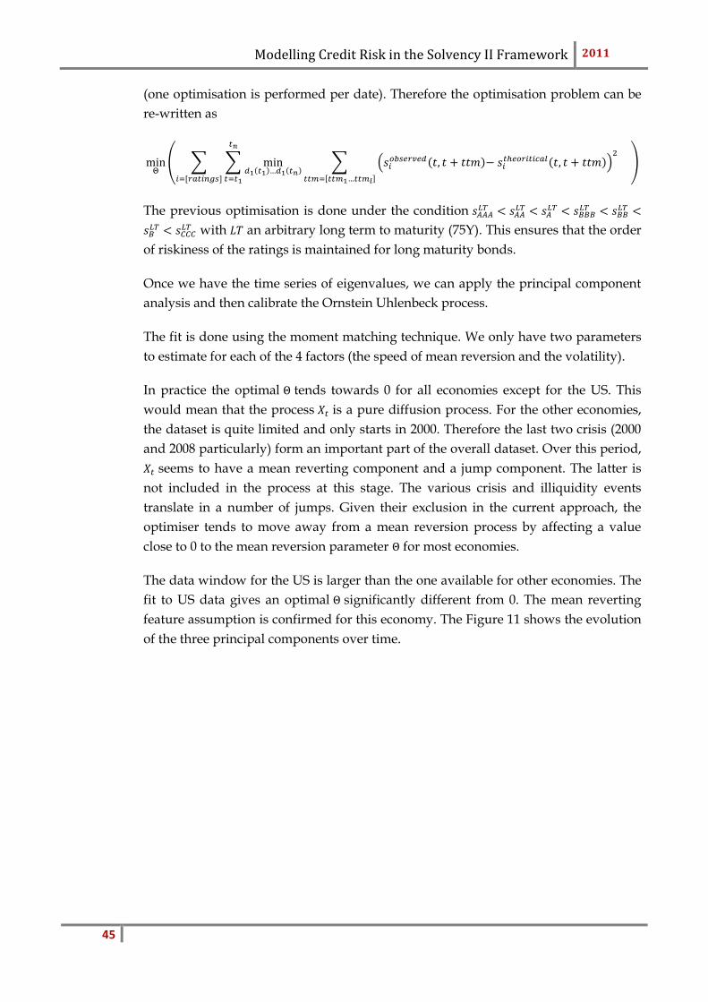
Modelling Credit Risk in the Solvency II Framework 2011
45
(one optimisation is performed per date). Therefore the optimisation problem can be
re-written as
The previous optimisation is done under the condition
with an arbitrary long term to maturity (75Y). This ensures that the order
of riskiness of the ratings is maintained for long maturity bonds.
Once we have the time series of eigenvalues, we can apply the principal component
analysis and then calibrate the Ornstein Uhlenbeck process.
The fit is done using the moment matching technique. We only have two parameters
to estimate for each of the 4 factors (the speed of mean reversion and the volatility).
In practice the optimal tends towards 0 for all economies except for the US. This
would mean that the process is a pure diffusion process. For the other economies,
the dataset is quite limited and only starts in 2000. Therefore the last two crisis (2000
and 2008 particularly) form an important part of the overall dataset. Over this period,
seems to have a mean reverting component and a jump component. The latter is
not included in the process at this stage. The various crisis and illiquidity events
translate in a number of jumps. Given their exclusion in the current approach, the
optimiser tends to move away from a mean reversion process by affecting a value
close to 0 to the mean reversion parameter for most economies.
The data window for the US is larger than the one available for other economies. The
fit to US data gives an optimal significantly different from 0. The mean reverting
feature assumption is confirmed for this economy. The Figure 11 shows the evolution
of the three principal components over time.
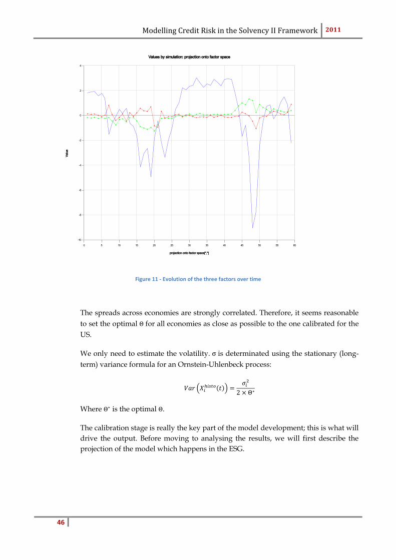
Modelling Credit Risk in the Solvency II Framework 2011
46
Figure 11 - Evolution of the three factors over time
The spreads across economies are strongly correlated. Therefore, it seems reasonable
to set the optimal for all economies as close as possible to the one calibrated for the
US.
We only need to estimate the volatility. is determinated using the stationary (long-
term) variance formula for an Ornstein-Uhlenbeck process:
Where is the optimal .
The calibration stage is really the key part of the model development; this is what will
drive the output. Before moving to analysing the results, we will first describe the
projection of the model which happens in the ESG.
Values by simulation: projection onto factor space
-10
-8
-6
-4
-2
0
2
4
0 5 10 15 20 25 30 35 40 45 50 55 60
projection onto factor space[*,*]
Valu
e
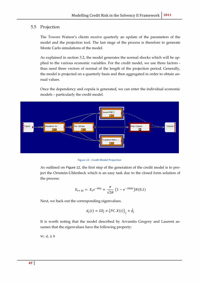
Modelling Credit Risk in the Solvency II Framework 2011
47
5.5 Projection
The Towers Watson’s clients receive quarterly an update of the parameters of the
model and the projection tool. The last stage of the process is therefore to generate
Monte Carlo simulations of the model.
As explained in section 3.2, the model generates the normal shocks which will be ap-
plied to the various economic variables. For the credit model, we use three factors -
thus need three vectors of normal of the length of the projection period. Generally,
the model is projected on a quarterly basis and then aggregated in order to obtain an-
nual values.
Once the dependency and copula is generated, we can enter the individual economic
models – particularly the credit model.
Figure 12 - Credit Model Projection
As outlined on Figure 12, the first step of the generation of the credit model is to pro-
ject the Ornstein-Uhlenbeck which is an easy task due to the closed form solution of
the process:
Next, we back out the corresponding eigenvalues.
It is worth noting that the model described by Arvanitis Gregory and Laurent as-
sumes that the eigenvalues have the following property:

Modelling Credit Risk in the Solvency II Framework 2011
48
It is not possible to enforce that the projected eigenvalues are all negative when we
recover them from the Ornstein-Uhlenbeck processes and the principal components.
Therefore, we need to amend the X processes. A new set of eigenvalues
Δ j 8 is defined, respecting the negativity feature.
Δ Δ
With Δ the originally simulated eigenvalues.
We can then obtain a modified process for X which fulfils the condition. The are
defined as
]
By doing this adjustment, we are breaking the autoregressive process and deviate
from the original process. This is mathematically incorrect but absolutely necessary in
order to limit the number of negative spreads. Furthermore, by amending the X proc-
ess slightly, we deviate from the mean imposed in the calibration which has a slight
impact on the long term mean of credit spreads.
The next stage of the projection is to calculate the variance of the model.
The same formula is used in the calculation of the transition matrices and the spreads.
Figure 12 - Credit Model Projection shows the credit model projection. The base unit
called “Spread RN” is where spreads are projected. Similarly, the base unit “Transi-
tion Matrix” generates the matrices for each projection date.
The spreads are easily computed using the formulas outlined in section 5.2. The
transition matrices are calculated using the results mentioned in section 5.3. The only
difference between these two calculations is the risk premium. Furthermore, as
explained in section 5.3, the X process is rescaled before being used in the calculation
of the transition matrices in order to reduce the volatility of the probabilities of
default – please refer to Table 4 in the results section.
The projection of the model is fairly fast. It is part of the Economic Scenario
Generators. We will now move to analysing the model and how good the results are
compared to other approaches.
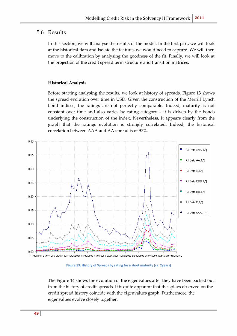
Modelling Credit Risk in the Solvency II Framework 2011
49
5.6 Results
In this section, we will analyse the results of the model. In the first part, we will look
at the historical data and isolate the features we would need to capture. We will then
move to the calibration by analysing the goodness of the fit. Finally, we will look at
the projection of the credit spread term structure and transition matrices.
Historical Analysis
Before starting analysing the results, we look at history of spreads. Figure 13 shows
the spread evolution over time in USD. Given the construction of the Merrill Lynch
bond indices, the ratings are not perfectly comparable. Indeed, maturity is not
constant over time and also varies by rating category – it is driven by the bonds
underlying the construction of the index. Nevertheless, it appears clearly from the
graph that the ratings evolution is strongly correlated. Indeed, the historical
correlation between AAA and AA spread is of 97%.
Figure 13: History of Spreads by rating for a short maturity (ca. 2years)
The Figure 14 shows the evolution of the eigenvalues after they have been backed out
from the history of credit spreads. It is quite apparent that the spikes observed on the
credit spread history coincide with the eigenvalues graph. Furthermore, the
eigenvalues evolve closely together.
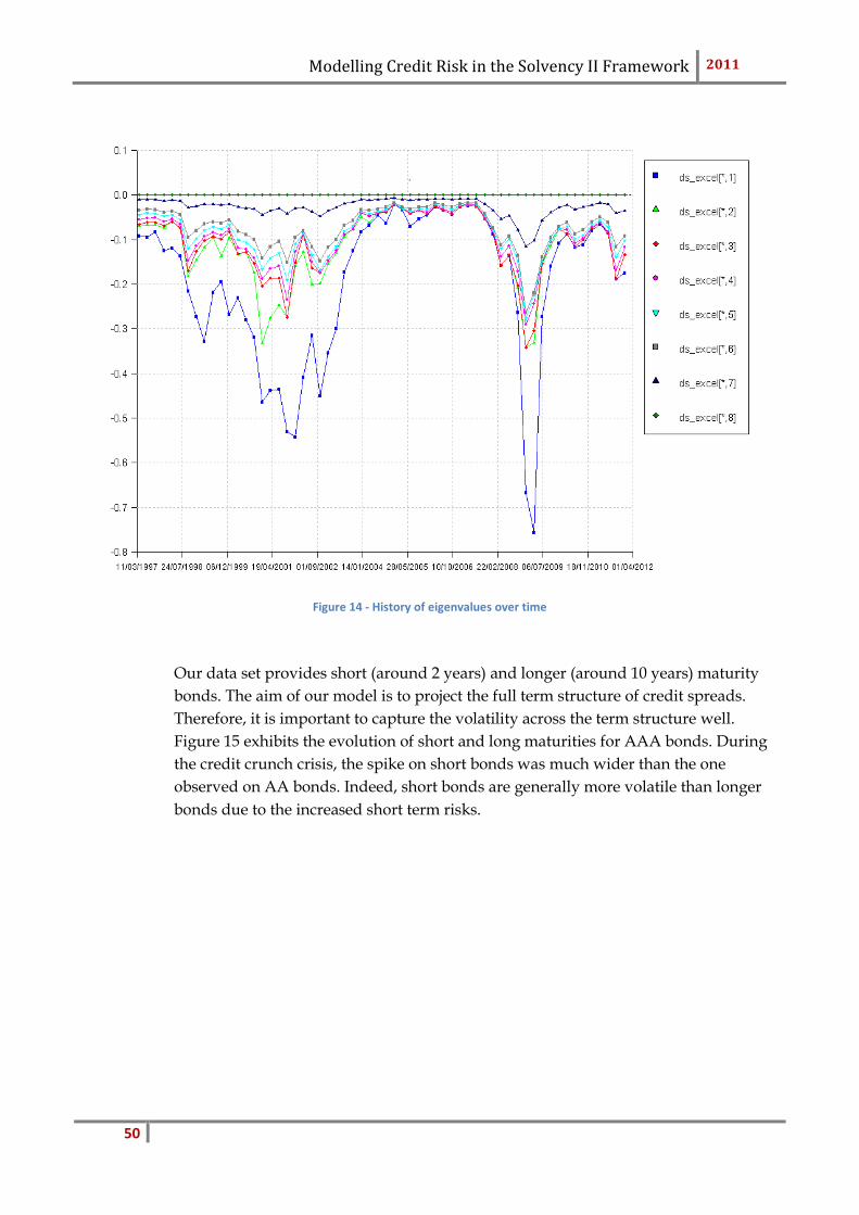
Modelling Credit Risk in the Solvency II Framework 2011
50
Figure 14 - History of eigenvalues over time
Our data set provides short (around 2 years) and longer (around 10 years) maturity
bonds. The aim of our model is to project the full term structure of credit spreads.
Therefore, it is important to capture the volatility across the term structure well.
Figure 15 exhibits the evolution of short and long maturities for AAA bonds. During
the credit crunch crisis, the spike on short bonds was much wider than the one
observed on AA bonds. Indeed, short bonds are generally more volatile than longer
bonds due to the increased short term risks.
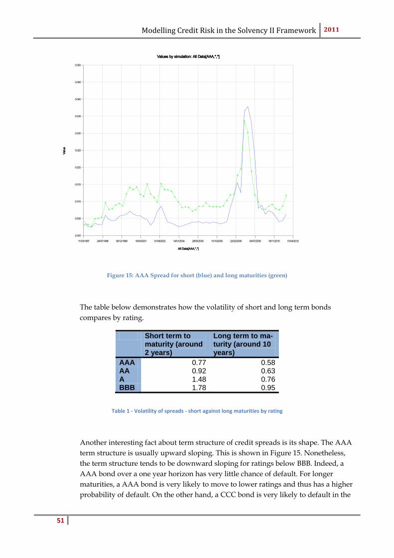
Modelling Credit Risk in the Solvency II Framework 2011
51
Figure 15: AAA Spread for short (blue) and long maturities (green)
The table below demonstrates how the volatility of short and long term bonds
compares by rating.
Short term to maturity (around 2 years)
Long term to ma-turity (around 10 years)
AAA 0.77 0.58 AA 0.92 0.63 A 1.48 0.76 BBB 1.78 0.95
Table 1 - Volatility of spreads - short against long maturities by rating
Another interesting fact about term structure of credit spreads is its shape. The AAA
term structure is usually upward sloping. This is shown in Figure 15. Nonetheless,
the term structure tends to be downward sloping for ratings below BBB. Indeed, a
AAA bond over a one year horizon has very little chance of default. For longer
maturities, a AAA bond is very likely to move to lower ratings and thus has a higher
probability of default. On the other hand, a CCC bond is very likely to default in the
Values by simulation: All Data[AAA,*,*]
0.000
0.005
0.010
0.015
0.020
0.025
0.030
0.035
0.040
0.045
0.050
11/03/1997 24/07/1998 06/12/1999 19/04/2001 01/09/2002 14/01/2004 28/05/2005 10/10/2006 22/02/2008 06/07/2009 18/11/2010 01/04/2012
All Data[AAA,*,*]
Valu
e
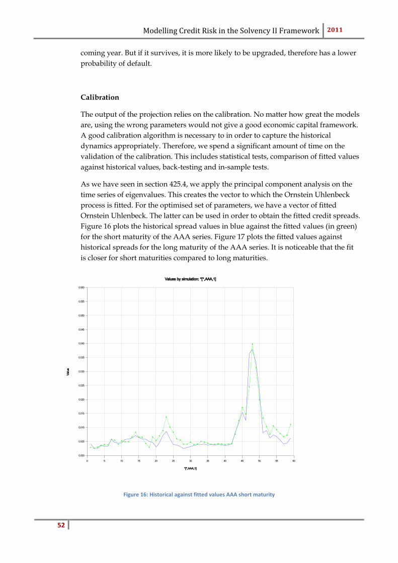
Modelling Credit Risk in the Solvency II Framework 2011
52
coming year. But if it survives, it is more likely to be upgraded, therefore has a lower
probability of default.
Calibration
The output of the projection relies on the calibration. No matter how great the models
are, using the wrong parameters would not give a good economic capital framework.
A good calibration algorithm is necessary to in order to capture the historical
dynamics appropriately. Therefore, we spend a significant amount of time on the
validation of the calibration. This includes statistical tests, comparison of fitted values
against historical values, back-testing and in-sample tests.
As we have seen in section 425.4, we apply the principal component analysis on the
time series of eigenvalues. This creates the vector to which the Ornstein Uhlenbeck
process is fitted. For the optimised set of parameters, we have a vector of fitted
Ornstein Uhlenbeck. The latter can be used in order to obtain the fitted credit spreads.
Figure 16 plots the historical spread values in blue against the fitted values (in green)
for the short maturity of the AAA series. Figure 17 plots the fitted values against
historical spreads for the long maturity of the AAA series. It is noticeable that the fit
is closer for short maturities compared to long maturities.
Figure 16: Historical against fitted values AAA short maturity
Values by simulation: *[*,AAA,1]
0.000
0.005
0.010
0.015
0.020
0.025
0.030
0.035
0.040
0.045
0.050
0.055
0.060
0 5 10 15 20 25 30 35 40 45 50 55 60
*[*,AAA,1]
Valu
e

Modelling Credit Risk in the Solvency II Framework 2011
53
Figure 17: Historical against fitted values AAA long maturity
An important ability of this model is to fit to the starting term structure of credit
spreads. We will now analyse how close this fit is. We look at the squared differences
between historical spreads and fitted values obtained in the model and at the sum of
squared differences in order to compare the various stages of the calibration process.
The numbers mentioned here are meaningless but are important tools for the
comparison of the various approaches.
At the first stage of calibration, we back out the history of eigenvalues from historical
credit spreads. Some mismatch appears already at that stage due to the lack of
freedom. We only have seven eigenvalues available in order to fit two maturities
across seven ratings. Therefore, the estimated eigenvalues imply certain spreads
which are not exactly in line with historical spreads.
The sum of squared errors as at September 2011 is around 0,10. At the second stage of
calibration, we apply the principal component analysis and isolate the three main
drivers of the eigenvalues. When moving to three components, some information will
be lost again. The sum of squared error is about 0,65. This error can be further
reduced when introducing a fourth principal component. It reduces to 0,4.
Depending on the economy this difference is more or less significant. It is arguable
that one could move to four factors in order to retain information and to better match
the starting term structure may be advisable.
Values by simulation: *[*,AAA,2]
0.000
0.005
0.010
0.015
0.020
0.025
0.030
0.035
0.040
0.045
0.050
0.055
0.060
0 5 10 15 20 25 30 35 40 45 50 55 60
*[*,AAA,2]
Valu
e
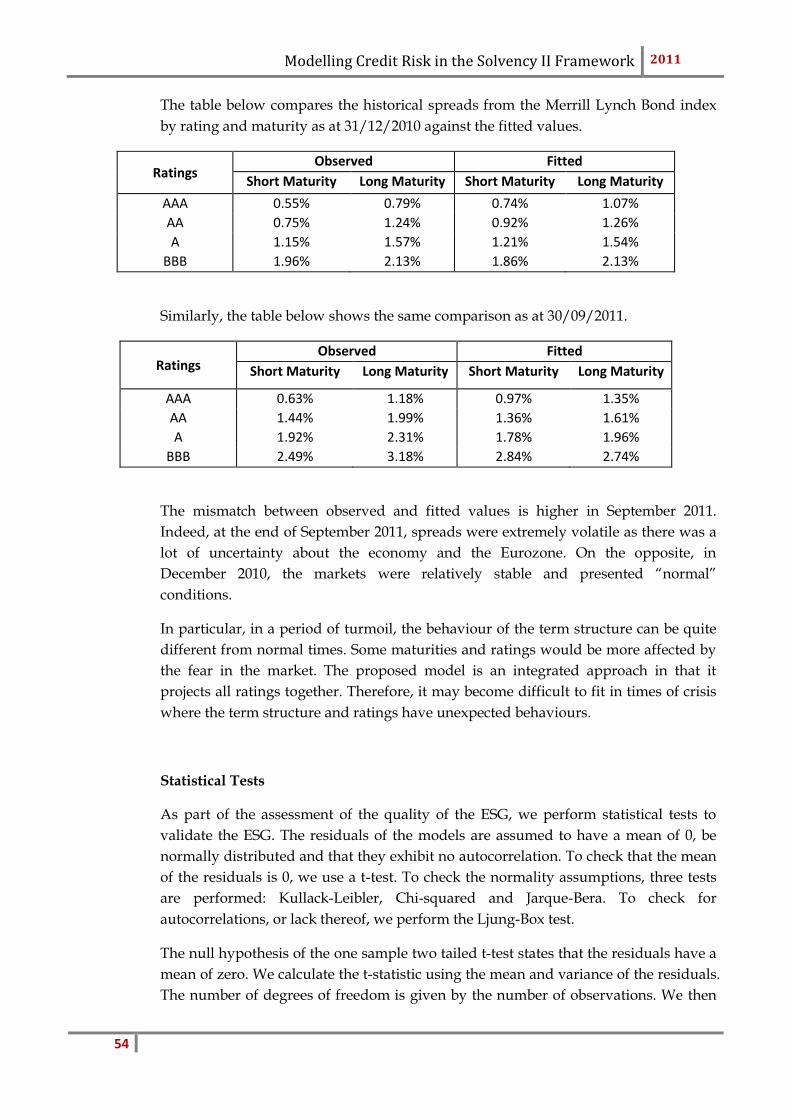
Modelling Credit Risk in the Solvency II Framework 2011
54
The table below compares the historical spreads from the Merrill Lynch Bond index
by rating and maturity as at 31/12/2010 against the fitted values.
Ratings Observed Fitted
Short Maturity Long Maturity Short Maturity Long Maturity
AAA 0.55% 0.79% 0.74% 1.07%
AA 0.75% 1.24% 0.92% 1.26%
A 1.15% 1.57% 1.21% 1.54%
BBB 1.96% 2.13% 1.86% 2.13%
Similarly, the table below shows the same comparison as at 30/09/2011.
Ratings Observed Fitted
Short Maturity Long Maturity Short Maturity Long Maturity
AAA 0.63% 1.18% 0.97% 1.35%
AA 1.44% 1.99% 1.36% 1.61%
A 1.92% 2.31% 1.78% 1.96%
BBB 2.49% 3.18% 2.84% 2.74%
The mismatch between observed and fitted values is higher in September 2011.
Indeed, at the end of September 2011, spreads were extremely volatile as there was a
lot of uncertainty about the economy and the Eurozone. On the opposite, in
December 2010, the markets were relatively stable and presented “normal”
conditions.
In particular, in a period of turmoil, the behaviour of the term structure can be quite
different from normal times. Some maturities and ratings would be more affected by
the fear in the market. The proposed model is an integrated approach in that it
projects all ratings together. Therefore, it may become difficult to fit in times of crisis
where the term structure and ratings have unexpected behaviours.
Statistical Tests
As part of the assessment of the quality of the ESG, we perform statistical tests to
validate the ESG. The residuals of the models are assumed to have a mean of 0, be
normally distributed and that they exhibit no autocorrelation. To check that the mean
of the residuals is 0, we use a t-test. To check the normality assumptions, three tests
are performed: Kullack-Leibler, Chi-squared and Jarque-Bera. To check for
autocorrelations, or lack thereof, we perform the Ljung-Box test.
The null hypothesis of the one sample two tailed t-test states that the residuals have a
mean of zero. We calculate the t-statistic using the mean and variance of the residuals.
The number of degrees of freedom is given by the number of observations. We then
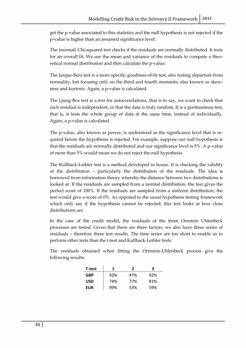
Modelling Credit Risk in the Solvency II Framework 2011
55
get the p-value associated to this statistics and the null hypothesis is not rejected if the
p-value is higher than an assumed significance level.
The (normal) Chi-squared test checks if the residuals are normally distributed. It tests
for an overall fit. We use the mean and variance of the residuals to compute a theo-
retical normal distribution and then calculate the p-value.
The Jarque-Bera test is a more specific goodness-of-fit test, also testing departure from
normality, but focusing only on the third and fourth moments, also known as skew-
ness and kurtosis. Again, a p-value is calculated.
The Ljung-Box test is a test for autocorrelations, that is to say, we want to check that
each residual is independent, or that the data is truly random. It is a portmanteau test,
that is, it tests the whole group of data at the same time, instead of individually.
Again, a p-value is calculated.
The p-value, also known as power, is understood as the significance level that is re-
quired before the hypothesis is rejected. For example, suppose our null hypothesis is
that the residuals are normally distributed and our significance level is 5%. A p-value
of more than 5% would mean we do not reject the null hypothesis.
The Kullback-Leibler test is a method developed in house. It is checking the validity
of the distribution – particularly the distribution of the residuals. The idea is
borrowed from information theory whereby the distance between two distributions is
looked at. If the residuals are sampled from a normal distribution, the test gives the
perfect score of 100%. If the residuals are sampled from a uniform distribution, the
test would give a score of 0%. As opposed to the usual hypothesis testing framework
which only say if the hypothesis cannot be rejected, this test looks at how close
distributions are.
In the case of the credit model, the residuals of the three Ornstein Uhlenbeck
processes are tested. Given that there are three factors, we also have three series of
residuals – therefore three test results. The time series are too short to enable us to
perform other tests than the t-test and Kullback-Leibler tests.
The residuals obtained when fitting the Ornstein-Uhlenbeck process give the
following results:
T-test 1 2 3
GBP 93% 47% 92%
USD 74% 77% 81%
EUR 99% 53% 59%
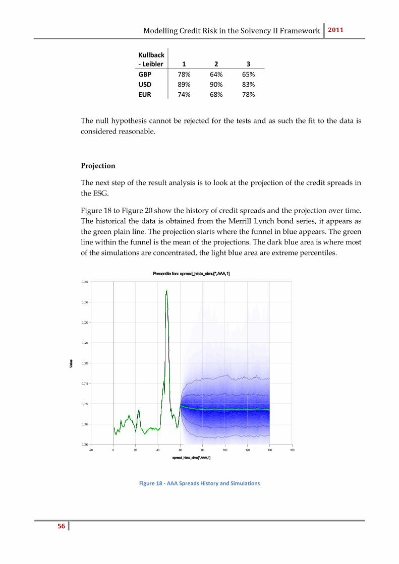
Modelling Credit Risk in the Solvency II Framework 2011
56
Kullback - Leibler 1 2 3
GBP 78% 64% 65%
USD 89% 90% 83%
EUR 74% 68% 78%
The null hypothesis cannot be rejected for the tests and as such the fit to the data is
considered reasonable.
Projection
The next step of the result analysis is to look at the projection of the credit spreads in
the ESG.
Figure 18 to Figure 20 show the history of credit spreads and the projection over time.
The historical the data is obtained from the Merrill Lynch bond series, it appears as
the green plain line. The projection starts where the funnel in blue appears. The green
line within the funnel is the mean of the projections. The dark blue area is where most
of the simulations are concentrated, the light blue area are extreme percentiles.
Figure 18 - AAA Spreads History and Simulations
Percentile fan: spread_histo_simu[*,AAA,1]
0.000
0.005
0.010
0.015
0.020
0.025
0.030
0.035
0.040
-20 0 20 40 60 80 100 120 140 160
spread_histo_simu[*,AAA,1]
Valu
e
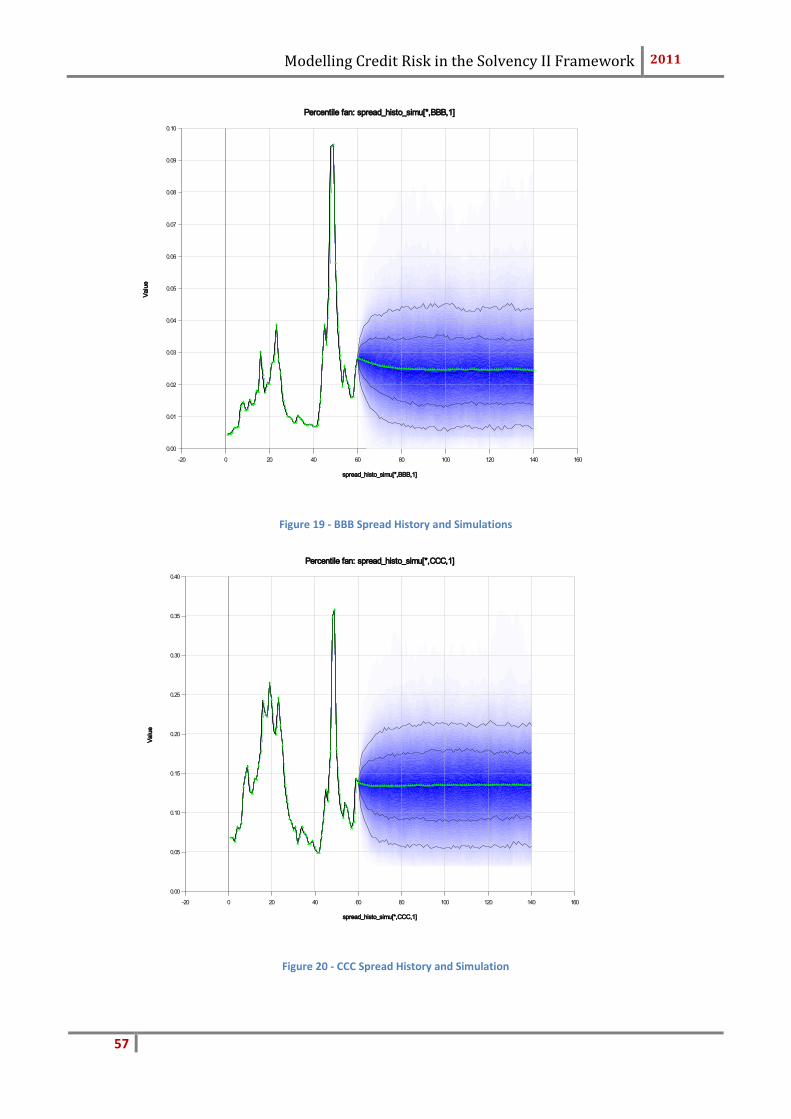
Modelling Credit Risk in the Solvency II Framework 2011
57
Figure 19 - BBB Spread History and Simulations
Figure 20 - CCC Spread History and Simulation
Percentile fan: spread_histo_simu[*,BBB,1]
0.00
0.01
0.02
0.03
0.04
0.05
0.06
0.07
0.08
0.09
0.10
-20 0 20 40 60 80 100 120 140 160
spread_histo_simu[*,BBB,1]
Valu
e
Percentile fan: spread_histo_simu[*,CCC,1]
0.00
0.05
0.10
0.15
0.20
0.25
0.30
0.35
0.40
-20 0 20 40 60 80 100 120 140 160
spread_histo_simu[*,CCC,1]
Valu
e
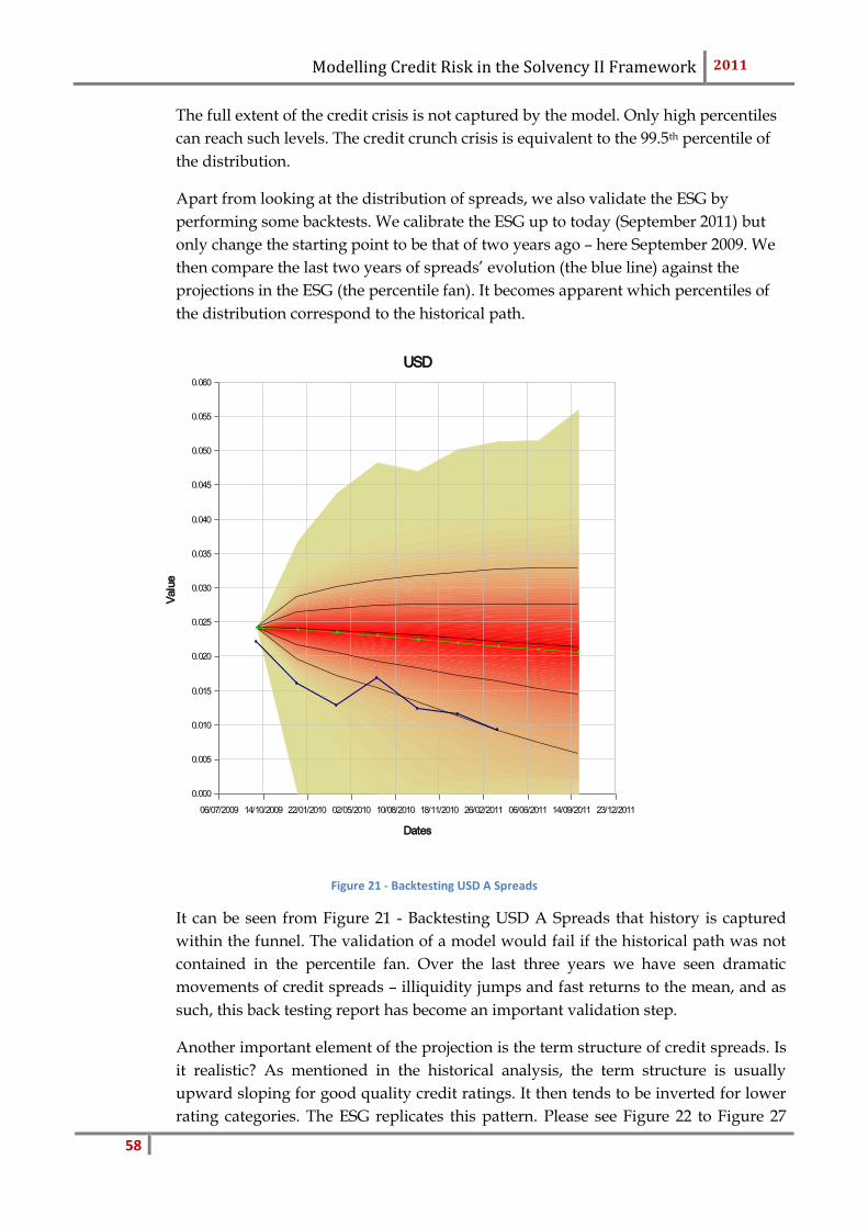
Modelling Credit Risk in the Solvency II Framework 2011
58
The full extent of the credit crisis is not captured by the model. Only high percentiles
can reach such levels. The credit crunch crisis is equivalent to the 99.5th percentile of
the distribution.
Apart from looking at the distribution of spreads, we also validate the ESG by
performing some backtests. We calibrate the ESG up to today (September 2011) but
only change the starting point to be that of two years ago – here September 2009. We
then compare the last two years of spreads’ evolution (the blue line) against the
projections in the ESG (the percentile fan). It becomes apparent which percentiles of
the distribution correspond to the historical path.
Figure 21 - Backtesting USD A Spreads
It can be seen from Figure 21 - Backtesting USD A Spreads that history is captured
within the funnel. The validation of a model would fail if the historical path was not
contained in the percentile fan. Over the last three years we have seen dramatic
movements of credit spreads – illiquidity jumps and fast returns to the mean, and as
such, this back testing report has become an important validation step.
Another important element of the projection is the term structure of credit spreads. Is
it realistic? As mentioned in the historical analysis, the term structure is usually
upward sloping for good quality credit ratings. It then tends to be inverted for lower
rating categories. The ESG replicates this pattern. Please see Figure 22 to Figure 27
USD
0.000
0.005
0.010
0.015
0.020
0.025
0.030
0.035
0.040
0.045
0.050
0.055
0.060
06/07/2009 14/10/2009 22/01/2010 02/05/2010 10/08/2010 18/11/2010 26/02/2011 06/06/2011 14/09/2011 23/12/2011
Dates
Valu
e
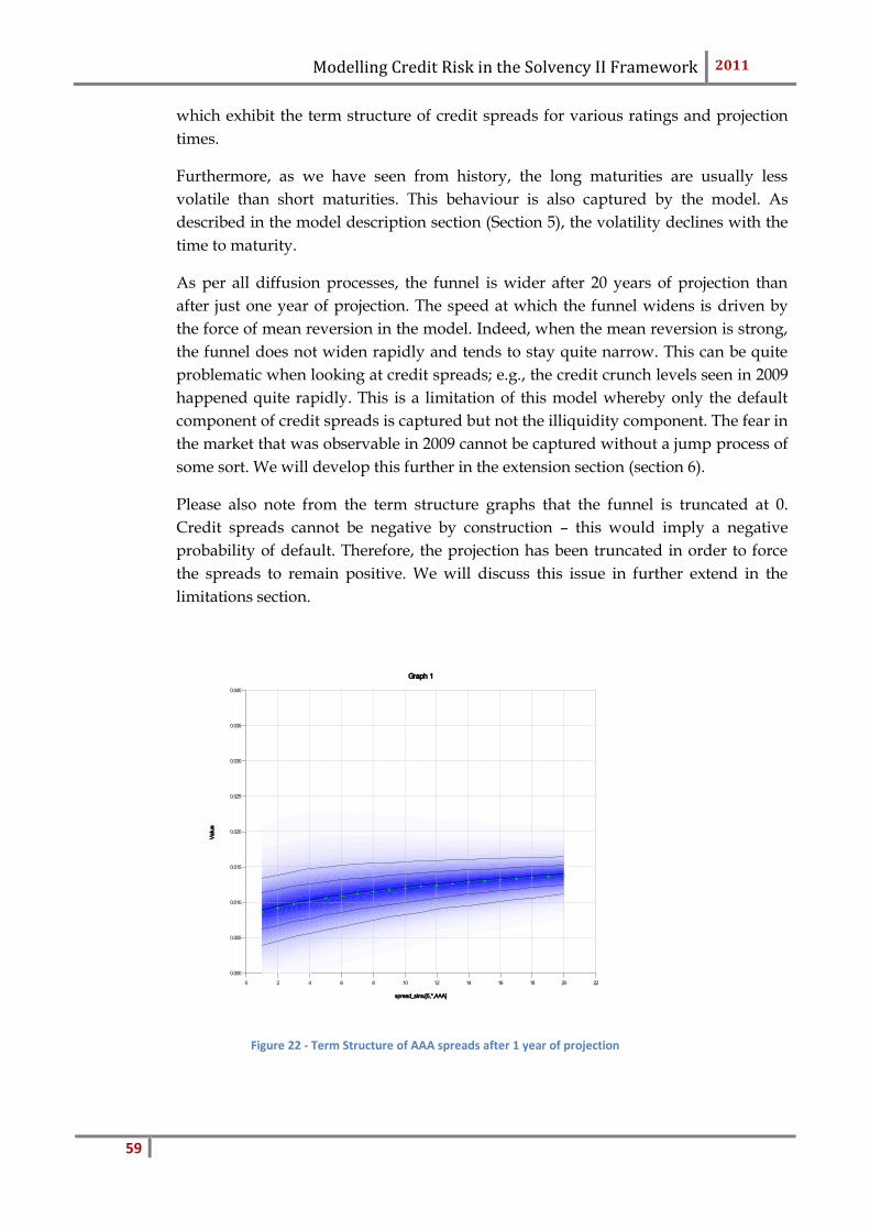
Modelling Credit Risk in the Solvency II Framework 2011
59
which exhibit the term structure of credit spreads for various ratings and projection
times.
Furthermore, as we have seen from history, the long maturities are usually less
volatile than short maturities. This behaviour is also captured by the model. As
described in the model description section (Section 5), the volatility declines with the
time to maturity.
As per all diffusion processes, the funnel is wider after 20 years of projection than
after just one year of projection. The speed at which the funnel widens is driven by
the force of mean reversion in the model. Indeed, when the mean reversion is strong,
the funnel does not widen rapidly and tends to stay quite narrow. This can be quite
problematic when looking at credit spreads; e.g., the credit crunch levels seen in 2009
happened quite rapidly. This is a limitation of this model whereby only the default
component of credit spreads is captured but not the illiquidity component. The fear in
the market that was observable in 2009 cannot be captured without a jump process of
some sort. We will develop this further in the extension section (section 6).
Please also note from the term structure graphs that the funnel is truncated at 0.
Credit spreads cannot be negative by construction – this would imply a negative
probability of default. Therefore, the projection has been truncated in order to force
the spreads to remain positive. We will discuss this issue in further extend in the
limitations section.
Figure 22 - Term Structure of AAA spreads after 1 year of projection
Graph 1
0.000
0.005
0.010
0.015
0.020
0.025
0.030
0.035
0.040
0 2 4 6 8 10 12 14 16 18 20 22
spread_simu[5,*,AAA]
Valu
e
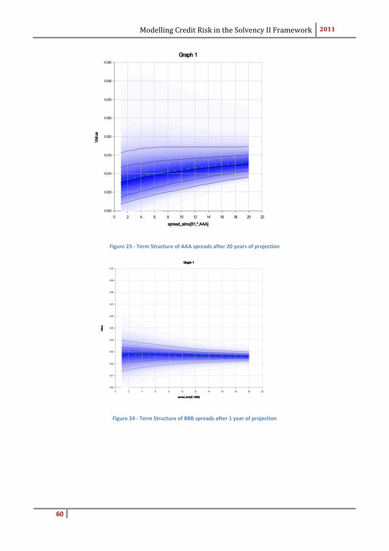
Modelling Credit Risk in the Solvency II Framework 2011
60
Figure 23 - Term Structure of AAA spreads after 20 years of projection
Figure 24 - Term Structure of BBB spreads after 1 year of projection
Graph 1
0.000
0.005
0.010
0.015
0.020
0.025
0.030
0.035
0.040
0 2 4 6 8 10 12 14 16 18 20 22
spread_simu[81,*,AAA]
Valu
e
Graph 1
0.00
0.01
0.02
0.03
0.04
0.05
0.06
0.07
0.08
0.09
0.10
0 2 4 6 8 10 12 14 16 18 20 22
spread_simu[5,*,BBB]
Valu
e
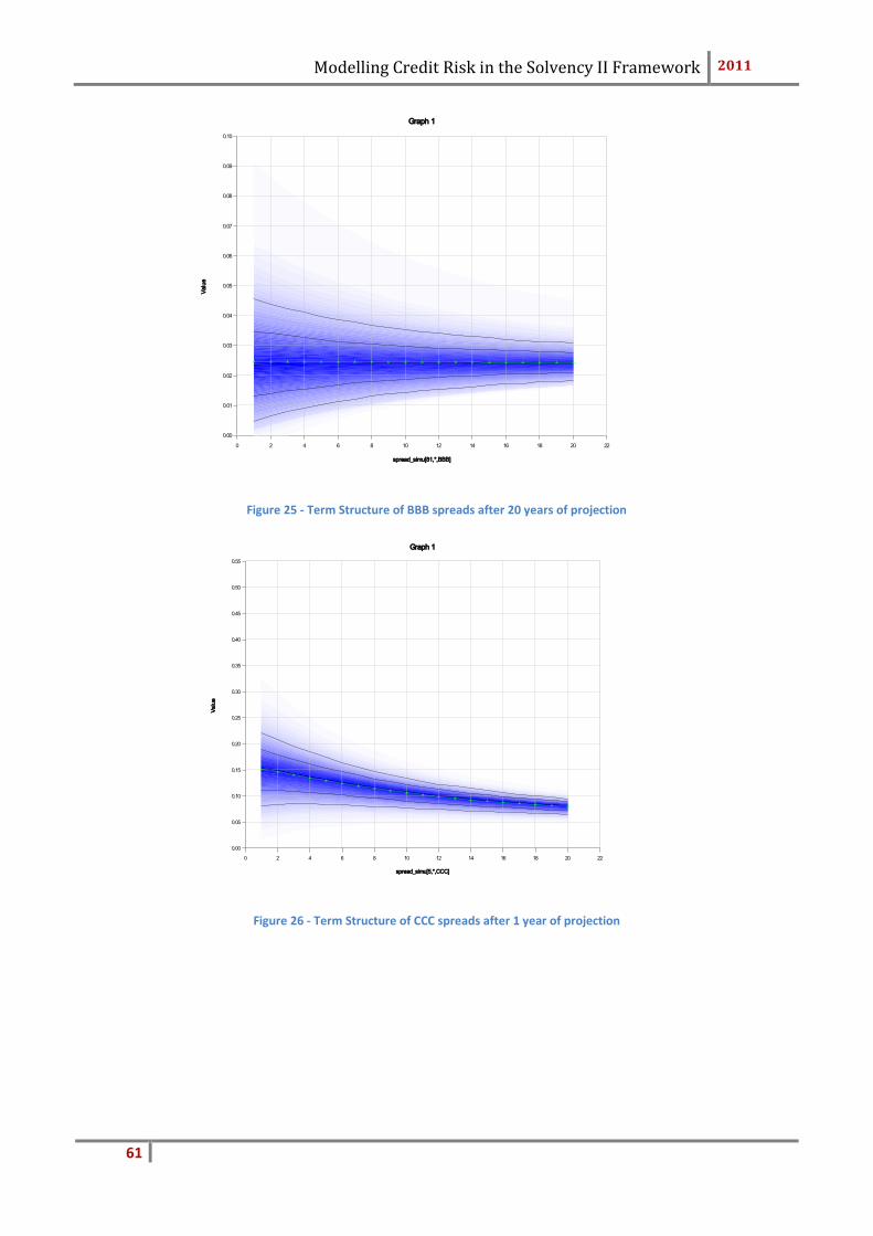
Modelling Credit Risk in the Solvency II Framework 2011
61
Figure 25 - Term Structure of BBB spreads after 20 years of projection
Figure 26 - Term Structure of CCC spreads after 1 year of projection
Graph 1
0.00
0.01
0.02
0.03
0.04
0.05
0.06
0.07
0.08
0.09
0.10
0 2 4 6 8 10 12 14 16 18 20 22
spread_simu[81,*,BBB]
Valu
e
Graph 1
0.00
0.05
0.10
0.15
0.20
0.25
0.30
0.35
0.40
0.45
0.50
0.55
0 2 4 6 8 10 12 14 16 18 20 22
spread_simu[5,*,CCC]
Valu
e
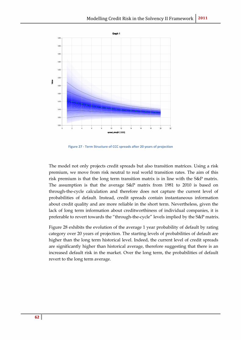
Modelling Credit Risk in the Solvency II Framework 2011
62
Figure 27 - Term Structure of CCC spreads after 20 years of projection
The model not only projects credit spreads but also transition matrices. Using a risk
premium, we move from risk neutral to real world transition rates. The aim of this
risk premium is that the long term transition matrix is in line with the S&P matrix.
The assumption is that the average S&P matrix from 1981 to 2010 is based on
through-the-cycle calculation and therefore does not capture the current level of
probabilities of default. Instead, credit spreads contain instantaneous information
about credit quality and are more reliable in the short term. Nevertheless, given the
lack of long term information about creditworthiness of individual companies, it is
preferable to revert towards the “through-the-cycle” levels implied by the S&P matrix.
Figure 28 exhibits the evolution of the average 1 year probability of default by rating
category over 20 years of projection. The starting levels of probabilities of default are
higher than the long term historical level. Indeed, the current level of credit spreads
are significantly higher than historical average, therefore suggesting that there is an
increased default risk in the market. Over the long term, the probabilities of default
revert to the long term average.
Graph 1
0.00
0.05
0.10
0.15
0.20
0.25
0.30
0.35
0.40
0.45
0.50
0.55
0 2 4 6 8 10 12 14 16 18 20 22
spread_simu[81,*,CCC]
Valu
e
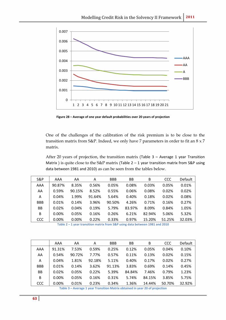
Modelling Credit Risk in the Solvency II Framework 2011
63
Figure 28 – Average of one year default probabilities over 20 years of projection
One of the challenges of the calibration of the risk premium is to be close to the
transition matrix from S&P. Indeed, we only have 7 parameters in order to fit an 8 x 7
matrix.
After 20 years of projection, the transition matrix (Table 3 – Average 1 year Transition
Matrix ) is quite close to the S&P matrix (Table 2 – 1 year transition matrix from S&P using
data between 1981 and 2010) as can be seen from the tables below.
S&P AAA AA A BBB BB B CCC Default
AAA 90.87% 8.35% 0.56% 0.05% 0.08% 0.03% 0.05% 0.01%
AA 0.59% 90.15% 8.52% 0.55% 0.06% 0.08% 0.02% 0.02%
A 0.04% 1.99% 91.64% 5.64% 0.40% 0.18% 0.02% 0.08%
BBB 0.01% 0.14% 3.96% 90.50% 4.26% 0.71% 0.16% 0.27%
BB 0.02% 0.04% 0.19% 5.79% 83.97% 8.09% 0.84% 1.05%
B 0.00% 0.05% 0.16% 0.26% 6.21% 82.94% 5.06% 5.32%
CCC 0.00% 0.00% 0.22% 0.33% 0.97% 15.20% 51.25% 32.03% Table 2 – 1 year transition matrix from S&P using data between 1981 and 2010
AAA AA A BBB BB B CCC Default
AAA 91.31% 7.53% 0.59% 0.25% 0.12% 0.05% 0.04% 0.10%
AA 0.54% 90.72% 7.77% 0.57% 0.11% 0.13% 0.02% 0.15%
A 0.04% 1.81% 92.18% 5.11% 0.40% 0.17% 0.02% 0.27%
BBB 0.01% 0.14% 3.62% 91.13% 3.83% 0.69% 0.14% 0.45%
BB 0.02% 0.05% 0.22% 5.39% 84.84% 7.46% 0.79% 1.23%
B 0.00% 0.05% 0.16% 0.31% 5.74% 84.15% 3.85% 5.75%
CCC 0.00% 0.01% 0.23% 0.34% 1.36% 14.44% 50.70% 32.92% Table 3 – Average 1 year Transition Matrix obtained in year 20 of projection
0
0.001
0.002
0.003
0.004
0.005
0.006
0.007
1 2 3 4 5 6 7 8 9 10 11 12 13 14 15 16 17 18 19 20 21
AAA
AA
A
BBB
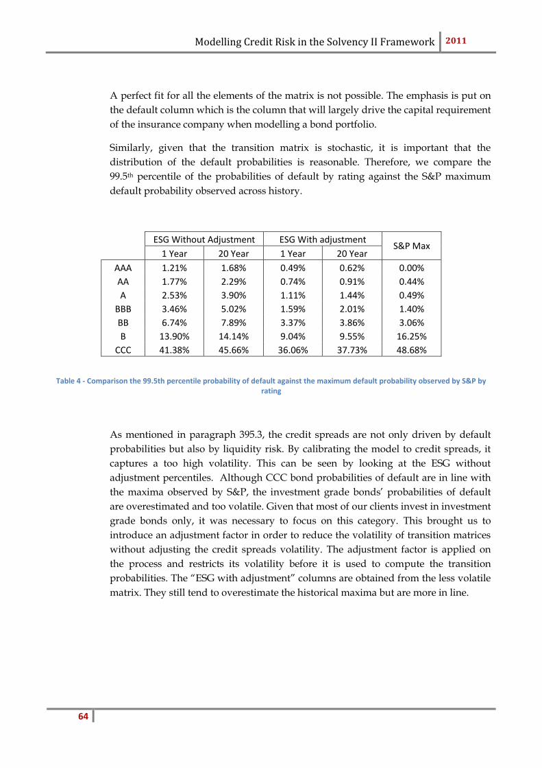
Modelling Credit Risk in the Solvency II Framework 2011
64
A perfect fit for all the elements of the matrix is not possible. The emphasis is put on
the default column which is the column that will largely drive the capital requirement
of the insurance company when modelling a bond portfolio.
Similarly, given that the transition matrix is stochastic, it is important that the
distribution of the default probabilities is reasonable. Therefore, we compare the
99.5th percentile of the probabilities of default by rating against the S&P maximum
default probability observed across history.
ESG Without Adjustment ESG With adjustment
S&P Max
1 Year 20 Year 1 Year 20 Year
AAA 1.21% 1.68% 0.49% 0.62% 0.00%
AA 1.77% 2.29% 0.74% 0.91% 0.44%
A 2.53% 3.90% 1.11% 1.44% 0.49%
BBB 3.46% 5.02% 1.59% 2.01% 1.40%
BB 6.74% 7.89% 3.37% 3.86% 3.06%
B 13.90% 14.14% 9.04% 9.55% 16.25%
CCC 41.38% 45.66% 36.06% 37.73% 48.68%
Table 4 - Comparison the 99.5th percentile probability of default against the maximum default probability observed by S&P by rating
As mentioned in paragraph 395.3, the credit spreads are not only driven by default
probabilities but also by liquidity risk. By calibrating the model to credit spreads, it
captures a too high volatility. This can be seen by looking at the ESG without
adjustment percentiles. Although CCC bond probabilities of default are in line with
the maxima observed by S&P, the investment grade bonds’ probabilities of default
are overestimated and too volatile. Given that most of our clients invest in investment
grade bonds only, it was necessary to focus on this category. This brought us to
introduce an adjustment factor in order to reduce the volatility of transition matrices
without adjusting the credit spreads volatility. The adjustment factor is applied on
the process and restricts its volatility before it is used to compute the transition
probabilities. The “ESG with adjustment” columns are obtained from the less volatile
matrix. They still tend to overestimate the historical maxima but are more in line.

Modelling Credit Risk in the Solvency II Framework 2011
65
5.7 Modelling a bond portfolio
The ultimate aim of the model is to provide a tool which projects portfolio returns
and calculates the capital requirement for the Solvency II requirement. As part of this
exercise, our clients want to model their bond portfolio.
So far, we discussed the projection of credit spreads and transition matrices which
happens in the ESG. We introduced the asset model in section 3.3. This is the critical
part of the model to downstream users; they are able to define their asset universe
and generate the returns of a bond portfolio. It is particularly important that the asset
model is developed in line with the ESG in order to benefit from its complexity. In-
deed, we have seen clients using the ESG but being unable to feed a stochastic transi-
tion matrix in their internal model.
In the case of corporate bonds, the asset model plays a major role. Indeed, the ESG
outputs credit spreads, nominal yield curves and transition matrices but not corpo-
rate bond returns as such. These are calculated in the asset model. In the latter, we
consider the income and capital return of each security on each valuation date over
the future periods under consideration. The returns for a period are determined by
valuing the bond at the previous valuation date, considering cash flows during the
period and then revaluing at the end of the period. The risk of rating migration from
one credit rating to another, upgrade or downgrade, (leading to a change in valuation,
due to the use of yield curves based on different ratings) and default is taken into ac-
count when calculating returns. Bonds are split into groups with the same seniority of
debt and initial credit rating, with each group belonging to an industry sector. Rating
category changes for individual bonds are simulated (based on the weights from the
transition matrix) and correlated with each other, via a correlation matrix by sector. It
is therefore possible to specify a correlation parameter for the correlation to be ap-
plied within each sector, and between each pair of sectors. These correlations are then
applied to each individual bond.
Rating category changes for each individual bond are also correlated to an "external
market variable", which in our model is taken as the overall equity return. Where
bonds are seen to default, it is assumed that they will still generate a certain propor-
tion of their future cash flows being the recovery rate proportion which is generated
from a Beta distribution1. The valuation of defaulted bonds is based upon these re-
duced future cash flows, using a yield curve corresponding to the rating of the bond
before it defaulted.
The mean and standard deviation for the recovery rates can be specified separately
for the various seniority levels of debt that the bonds can correspond to. In this way,
bonds from senior issues may be set to have a higher recovery rate than those of sub-
1 The use of the beta distribution is based on the paper CreditMetrics - Technical Document by JP Morgan. We parameterize the distribution using

Modelling Credit Risk in the Solvency II Framework 2011
66
ordinated issues. It is also possible to apply a correlation between the variability of
the recovery rates for defaulted bonds, and also a correlation between the recovery
rates of individual default bonds and the total number of defaults in the period.
5.8 Comparison with QIS 5
In section 2, we introduced the Solvency II framework. One of the suggest approaches
followed by insurance companies is the use of the Standard Formula. We described
the QIS 5 market risk calculation and its limitations – this is likely to become the Sol-
vency II method once it comes into force.
The alternative approach is to use the partial internal model. The Towers Watson
Portfolio Model calculates the Value at Risk of the portfolio for various risk levels (e.g.
1 in 200 year event) – clients then use it to calculate their capital requirement. The
portfolio model also breaks down the risk of the overall portfolio into risk categories
as required under Solvency II. The aim of this section is to look at the comparison be-
tween the QIS 5 result and the internal model result.
Please note that under QIS 5, the spread component of market risk is calculated is cal-
culated for a bond portfolio – indeed, it is the sum of weighted net asset values mul-
tiplied by a certain shock (up or down shocks). Therefore, we will compare the results
for a standard portfolio of an insurance company rather than comparing shocks to the
term structure of credit spreads.
For a portfolio with a total value of 500 million, the spread results are outlined below:
QIS 5 Internal Model
Spread Risk 11 million 20 million
Overall Portfolio 40 million 32 million
The internal model result is the standalone 1 in 200 value-at-risk.
For spread risk, the AGL model returns exhibits a value at risk that is significantly
higher than the QIS 5 number. However, at the overall portfolio level, the value at
risk is significantly less for the internal model compared the QIS 5 approach. This is
due to the diversification benefit obtained through the dependency structure of the
ESG. The internal model becomes more accurate. QIS 5 also accounts for correlation
between models but this is extremely limited.
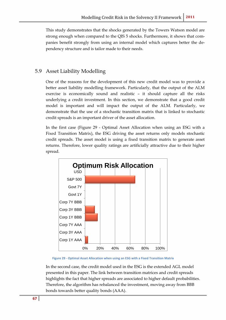
Modelling Credit Risk in the Solvency II Framework 2011
67
This study demonstrates that the shocks generated by the Towers Watson model are
strong enough when compared to the QIS 5 shocks. Furthermore, it shows that com-
panies benefit strongly from using an internal model which captures better the de-
pendency structure and is tailor made to their needs.
5.9 Asset Liability Modelling
One of the reasons for the development of this new credit model was to provide a
better asset liability modelling framework. Particularly, that the output of the ALM
exercise is economically sound and realistic – it should capture all the risks
underlying a credit investment. In this section, we demonstrate that a good credit
model is important and will impact the output of the ALM. Particularly, we
demonstrate that the use of a stochastic transition matrix that is linked to stochastic
credit spreads is an important driver of the asset allocation.
In the first case (Figure 29 - Optimal Asset Allocation when using an ESG with a
Fixed Transition Matrix), the ESG driving the asset returns only models stochastic
credit spreads. The asset model is using a fixed transition matrix to generate asset
returns. Therefore, lower quality ratings are artificially attractive due to their higher
spread.
Figure 29 - Optimal Asset Allocation when using an ESG with a Fixed Transition Matrix
In the second case, the credit model used in the ESG is the extended AGL model
presented in this paper. The link between transition matrices and credit spreads
highlights the fact that higher spreads are associated to higher default probabilities.
Therefore, the algorithm has rebalanced the investment, moving away from BBB
bonds towards better quality bonds (AAA).
0% 20% 40% 60% 80% 100%
Corp 1Y AAA
Corp 3Y AAA
Corp 7Y AAA
Corp 1Y BBB
Corp 3Y BBB
Corp 7Y BBB
Govt 1Y
Govt 7Y
S&P 500
USD
Optimum Risk Allocation
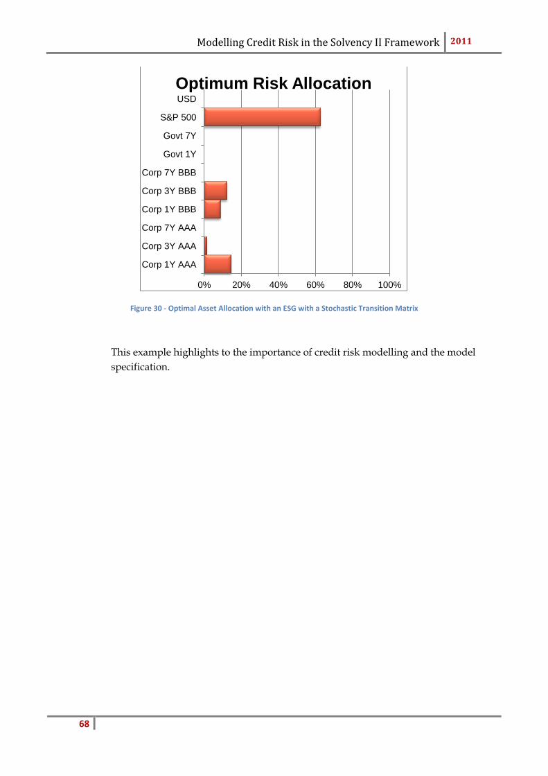
Modelling Credit Risk in the Solvency II Framework 2011
68
Figure 30 - Optimal Asset Allocation with an ESG with a Stochastic Transition Matrix
This example highlights to the importance of credit risk modelling and the model
specification.
0% 20% 40% 60% 80% 100%
Corp 1Y AAA
Corp 3Y AAA
Corp 7Y AAA
Corp 1Y BBB
Corp 3Y BBB
Corp 7Y BBB
Govt 1Y
Govt 7Y
S&P 500
USD
Optimum Risk Allocation
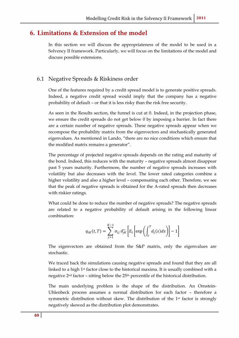
Modelling Credit Risk in the Solvency II Framework 2011
69
6. Limitations & Extension of the model
In this section we will discuss the appropriateness of the model to be used in a
Solvency II framework. Particularly, we will focus on the limitations of the model and
discuss possible extensions.
6.1 Negative Spreads & Riskiness order
One of the features required by a credit spread model is to generate positive spreads.
Indeed, a negative credit spread would imply that the company has a negative
probability of default – or that it is less risky than the risk free security.
As seen in the Results section, the funnel is cut at 0. Indeed, in the projection phase,
we ensure the credit spreads do not get below 0 by imposing a barrier. In fact there
are a certain number of negative spreads. These negative spreads appear when we
recompose the probability matrix from the eigenvectors and stochastically generated
eigenvalues. As mentioned in Lando, “there are no nice conditions which ensure that
the modified matrix remains a generator”.
The percentage of projected negative spreads depends on the rating and maturity of
the bond. Indeed, this reduces with the maturity – negative spreads almost disappear
past 5 years maturity. Furthermore, the number of negative spreads increases with
volatility but also decreases with the level. The lower rated categories combine a
higher volatility and also a higher level – compensating each other. Therefore, we see
that the peak of negative spreads is obtained for the A-rated spreads then decreases
with riskier ratings.
What could be done to reduce the number of negative spreads? The negative spreads
are related to a negative probability of default arising in the following linear
combination:
The eigenvectors are obtained from the S&P matrix, only the eigenvalues are
stochastic.
We traced back the simulations causing negative spreads and found that they are all
linked to a high 1st factor close to the historical maxima. It is usually combined with a
negative 2nd factor – sitting below the 25th percentile of the historical distribution.
The main underlying problem is the shape of the distribution. An Ornstein-
Uhlenbeck process assumes a normal distribution for each factor – therefore a
symmetric distribution without skew. The distribution of the 1st factor is strongly
negatively skewed as the distribution plot demonstrates.
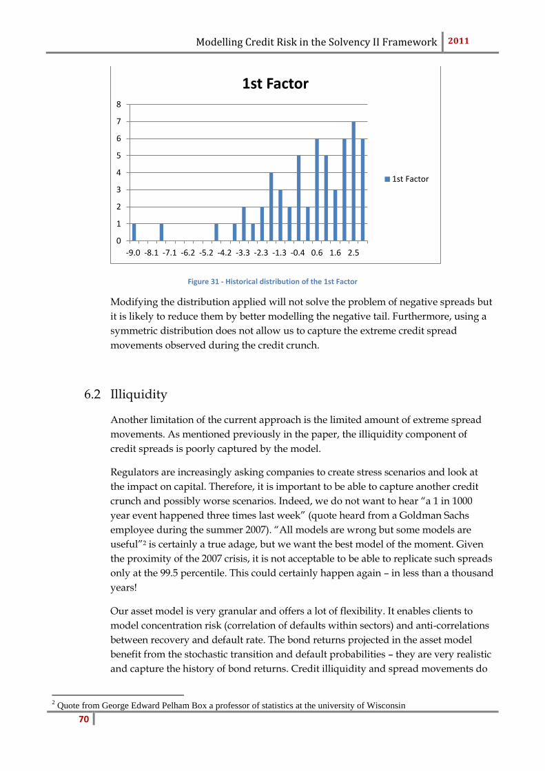
Modelling Credit Risk in the Solvency II Framework 2011
70
Figure 31 - Historical distribution of the 1st Factor
Modifying the distribution applied will not solve the problem of negative spreads but
it is likely to reduce them by better modelling the negative tail. Furthermore, using a
symmetric distribution does not allow us to capture the extreme credit spread
movements observed during the credit crunch.
6.2 Illiquidity
Another limitation of the current approach is the limited amount of extreme spread
movements. As mentioned previously in the paper, the illiquidity component of
credit spreads is poorly captured by the model.
Regulators are increasingly asking companies to create stress scenarios and look at
the impact on capital. Therefore, it is important to be able to capture another credit
crunch and possibly worse scenarios. Indeed, we do not want to hear “a 1 in 1000
year event happened three times last week” (quote heard from a Goldman Sachs
employee during the summer 2007). “All models are wrong but some models are
useful”2 is certainly a true adage, but we want the best model of the moment. Given
the proximity of the 2007 crisis, it is not acceptable to be able to replicate such spreads
only at the 99.5 percentile. This could certainly happen again – in less than a thousand
years!
Our asset model is very granular and offers a lot of flexibility. It enables clients to
model concentration risk (correlation of defaults within sectors) and anti-correlations
between recovery and default rate. The bond returns projected in the asset model
benefit from the stochastic transition and default probabilities – they are very realistic
and capture the history of bond returns. Credit illiquidity and spread movements do
2 Quote from George Edward Pelham Box a professor of statistics at the university of Wisconsin
0
1
2
3
4
5
6
7
8
-9.0 -8.1 -7.1 -6.2 -5.2 -4.2 -3.3 -2.3 -1.3 -0.4 0.6 1.6 2.5
1st Factor
1st Factor
Modelling Credit Risk in the Solvency II Framework 2011
71
not affect the return of the bond if the strategy is to hold to maturity – indeed, only
default occurrence would dampen redemption. During the credit crunch crisis,
spreads have jumped while default occurrence hasn’t changed as much
proportionally. From that angle, the volatility of spreads generated in the ESG should
not be source of worry but clients should focus on the validation of the bond returns.
Nevertheless, credit spread data is easier to observe and to compare to. Clients could
adopt a rebalancing strategy, in which case valuations of bonds matter as well.
Therefore, it is important to capture the periods of illiquidity.
Section 6.1 introduces the negative spreads occurrence and the poorly captured shape
of distribution of the first factor. A couple of alternatives exist in order to capture this
shape better. In their original paper, Arvanitis Gregory and Laurent suggest the use
of a CIR process. This has the advantage of having an asymmetric shape. However, it
is necessary to modify the principal components in order to apply such a process.
Indeed, the CIR ensures the process remains positive – therefore can only be
calibrated to a positive process. Of course, taking the exponential of the factors
described in this paper so far would be an alternative but the closed form solution
would be lost. Furthermore, the calibration is far from easy. Finally, applying the CIR
process to the factors does not ensure the spreads remain positive – this all comes
down to the principal components and their linear combination.
The aim of this section is to model the illiquidity component of credit spreads. In
essence, illiquidity events such as credit crunch crisis are better modelled as jumps.
There are a couple of possibilities in order to capture jumps.
Our first idea was to relax the normality assumption of residuals. It would be fairly
easy to calibrate a jump process to the residuals obtained from the initial Ornstein-
Uhlenbeck calibration. When studying the residuals, it is clear that the credit crunch
is poorly captured by the model. It is apparent that the first factor is the most
significant contributor to liquidity jumps. Indeed, in case of an illiquidity crisis, all
ratings tend to be affected in a proportional fashion. Therefore, we have focused our
attention on the first component.
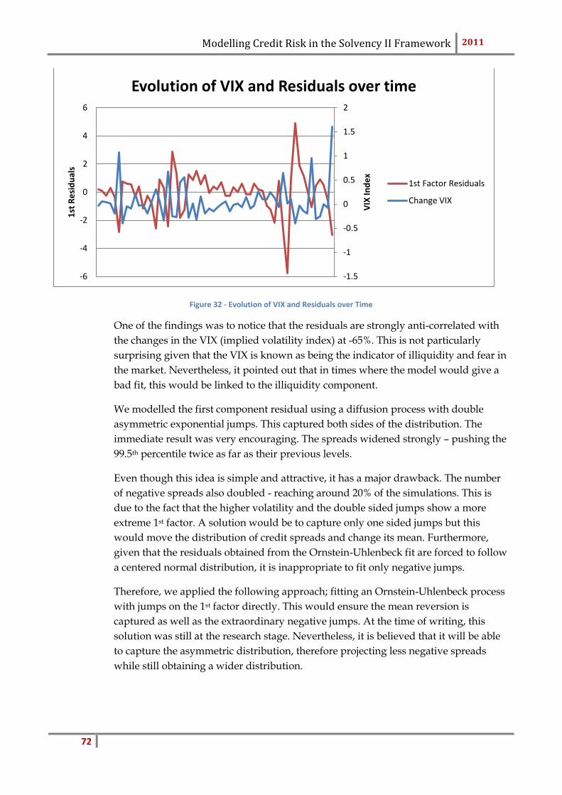
Modelling Credit Risk in the Solvency II Framework 2011
72
Figure 32 - Evolution of VIX and Residuals over Time
One of the findings was to notice that the residuals are strongly anti-correlated with
the changes in the VIX (implied volatility index) at -65%. This is not particularly
surprising given that the VIX is known as being the indicator of illiquidity and fear in
the market. Nevertheless, it pointed out that in times where the model would give a
bad fit, this would be linked to the illiquidity component.
We modelled the first component residual using a diffusion process with double
asymmetric exponential jumps. This captured both sides of the distribution. The
immediate result was very encouraging. The spreads widened strongly – pushing the
99.5th percentile twice as far as their previous levels.
Even though this idea is simple and attractive, it has a major drawback. The number
of negative spreads also doubled - reaching around 20% of the simulations. This is
due to the fact that the higher volatility and the double sided jumps show a more
extreme 1st factor. A solution would be to capture only one sided jumps but this
would move the distribution of credit spreads and change its mean. Furthermore,
given that the residuals obtained from the Ornstein-Uhlenbeck fit are forced to follow
a centered normal distribution, it is inappropriate to fit only negative jumps.
Therefore, we applied the following approach; fitting an Ornstein-Uhlenbeck process
with jumps on the 1st factor directly. This would ensure the mean reversion is
captured as well as the extraordinary negative jumps. At the time of writing, this
solution was still at the research stage. Nevertheless, it is believed that it will be able
to capture the asymmetric distribution, therefore projecting less negative spreads
while still obtaining a wider distribution.
-1.5
-1
-0.5
0
0.5
1
1.5
2
-6
-4
-2
0
2
4
6
VIX
Ind
ex
1st
Re
sid
ual
s
Evolution of VIX and Residuals over time
1st Factor Residuals
Change VIX
Modelling Credit Risk in the Solvency II Framework 2011
73
6.3 Sovereign Risk
The model described in this paper focuses on the credit risk of corporate bonds
particularly. Indeed, the asset model does not model government bond defaults. A
similar assumption is described in QIS5. For developed countries, it is common to
assume that government bonds do not have credit risk.
In 2011, the degradation of sovereign bond credit quality has raised concerns –
particularly in the Eurozone. Should capital model capture the risk of government
bonds defaulting? Should this be part of the internal model or should this be
modelled as a stress scenario?
The ESG is calibrated using statistical techniques and historical data. The number of
government bonds defaults in history is scarce and does not form sufficient database
for the calibration of a model. Instead, we suggest clients to use the flexibility of the
asset model. It is possible to enter the Euro government bonds as AA bonds or A
bonds in the corporate bond module. This would have a general impact on the capital
charge. Alternatively, we are developing a functionality allowing users to enter a rare
default event which would be modelled in the asset model – directly impacting
government returns.
The model described in this paper cannot be easily extended to capture government
bond spreads due to its necessary linkage to transition rates and defaults. No such
matrix is available for government bonds – even if it was, the default probabilities
would not be high enough to justify the current observed spreads.
Modelling Credit Risk in the Solvency II Framework 2011
74
7. Conclusion
As part of our work at Towers Watson, our aim is to help clients with their
regulatory submissions. Particularly, Solvency II brings up new requirements
to insurance companies.
One of the key risks faced by insurance companies is credit risk. It affects the
reinsurance business, the counterparties but most importantly the investment
risk. The aim of this paper was to review the approach introduced by QIS5 –
the preliminary study of the Solvency II framework – for modelling credit risk
and compare it to the literature.
There is a whole range of available approaches focusing on idiosyncratic or
systemic risk. One of which is the Jarrow, Lando and Turnbull framework. We
developed it further in order to be able to model credit spreads stochastically.
Furthermore, we wanted it to be applicable to risk management and the inter-
nal model of an insurance company.
The model introduced in this paper addresses most of the issues encountered
when modelling spreads but has a few limitations. A few extensions to the
model are introduced in section 6 in order to bring the framework to the next
level. Particularly, reducing the number of negative spreads and better captur-
ing the high spreads observed during the credit crunch.
Modelling Credit Risk in the Solvency II Framework 2011
75
8. Bibliography
ARVANITIS (Angelo), GREGORY (Jonathon), LAURENT (Jean-Paul), “Building Models for Credit Spreads”, in The Journal of Derivatives, Spring 1999, pp 27-43 BRIGO (Damiano), MERCURIO (Fabio), Interest Rate Models – Theory and Practice, Second Edition, Springer Finance, 2006 JARROW (Robert), LANDO (David), TURBNULL (Stuart), “A Markov Model for the Term Structure of Credit Risk Spreads”, in The Review of Financial Studies, Summer 1997 Vol. 10, No.2 LANDO (David), Credit Risk Modelling, Princeton University Press, 2004 De SERVIGNY (Arnaud), RENAULT (Olivier), Measuring and Managing Credit Risk, McGraw-Hill, 2004 FELSENHEIMER (Jochen), GISDAKIS (Philip), ZAISER (Michael), Active Credit Portfolio Management, Wiley, 2006 http://www.standardandpoors.com/ratings/articles/en/us/?assetID=1245302234237
MERTON (Robert), A dynamic general equilibrium model of the asset market and its application to
the pricing of the capital structure of the firm, 1970
VARNELL (Elliot), Economic scenario generators and Solvency II, Sessional meeting paper, 2009
https://eiopa.europa.eu/consultations/qis/quantitative-impact-study-5/index.html