Proceedings World Geothermal Congress 2020

Reykjavik, Iceland, April 26 – May 2, 2020

1

Depth-average Estimation of 1D Subsurface Resistivity from MT Data in Los Humeros

Geothermal Field, Mexico

Romo-Jones J.M.1, Avilés-Esquivel T.A.1, Arango-Galván C.2, Ruiz-Aguilar D. 1., Salas-Corrales J.L.2,

Benediktsdóttir A.3, Hersir G.P. 3

1 División de Ciencias de la Tierra, Centro de Investigación Científica y de Educación Superior de Ensenada (CICESE), Ensenada,

México. 2 Instituto de Geofísica, Universidad Nacional Autónoma de México (UNAM). 3 Iceland GeoSurvey (ISOR)

jromo@cicese.edu.mx

Keywords: Geothermal, Mexico, Los Humeros, electrical conductivity, magnetotellurics, 1D inversion, GEMex

ABSTRACT

Generally, the first stage in the interpretation of magnetotelluric data consists of the construction of 1D resistivity models, i.e.,

subsurface resistivity versus depth profiles. A commonly used approach is to estimate 1D models with minimal structural

complexity, frequently applying a data inversion scheme that uses the Occam´s razor principle. This type of algorithms uses the

measured data (apparent resistivity and phase) to produce a simple distribution of the subsurface resistivity versus depth. As the

solution is not unique, a given model is just one of a whole class of models that may fit the measurements equally well. Besides the

instability inherent in the inverse problem, the construction of models is based on measured data that are both inaccurate and

insufficient. Therefore, it is worthwhile to have some procedure to make statistical inferences about the goodness of the models, in

terms of their variance and depth-resolution. In this paper, we apply a known simple method to estimate depth averages of the

subsurface resistivity as well as their uncertainty and resolution. This approach uses only the apparent resistivity data and makes no

other assumption. We applied this scheme to magnetotelluric data measured in Los Humeros geothermal field, in Mexico, within

the frame of the GEMex project. Our estimations are shown together with the minimal-structure Occam-type models obtained from

the same data set, in such a way that we can appreciate the 1D resistivity model along with the variance of the subsurface resistivity

at different depths.

This abstract presents results of the GEMex Project, funded by the Mexican Energy Sustainability Fund CONACYT-SENER,

Project 2015-04-268074 and by the European Union’s Horizon 2020 research and innovation programe under grant agreement No.

727550. More information can be found on the GEMex Website: http://www.gemex-h2020.eu.

1. INTRODUCTION

In recent years the Mexican government promoted the development of geothermal energy as clean energy that can contribute to

reducing the use of fossil fuels for electricity generation. As part of this effort, it hosted research projects focused on the

investigation of unconventional resources. An example is the collaboration between Europe and Mexico named GEMex Project

(http://www.gemex-h2020.eu), which has activities in two geothermal areas: a low permeability system in Acoculco, Puebla, and in

Los Humeros geothermal field (LHGF) where superhot fluids are present. In order to improve the understanding of this system,

investigation of different physical properties of the subsurface rocks is required. The magnetotelluric geophysical method provides

information about the electrical conductivity of the rocks, mainly associated with the presence of fluids or hydrothermal alteration

zones. With this technique, subsurface conductivity is inferred from the natural electromagnetic fields measured at the Earth’s

surface, as their relative amplitude depends on the rock conductivity at depth. However, assessing a subsurface model from a data

set observed at the surface is a problem (inverse problem) that has not a unique solution. That means that more than one model can

explain equally well an observed dataset. Therefore, it is worthwhile to find methods to set statistical bounds to a model solution,

i.e. estimate the average conductivity and depth as well as their uncertainties. In this work, we calculated 1D resistivity models for

a magnetotelluric dataset measured in LHGF, using the statistical inference method proposed by Gómez-Treviño (1996) to estimate

depth averages of the subsurface resistivity as well as their uncertainty and resolution. Our results are compared with 1D models

obtained with Occam inversion algorithm by Constable et al. (1987). Knowing the mean value and the variance of the subsurface

resistivity gives insights about the goodness of the models, by assessing the accuracy of the estimations as well as determining the

depth resolution supported by the observed data.

2. THE LOS HUMEROS GEOLOGY

Los Humeros volcanic complex (LHVC) is in the northeastern sector of the Transverse-Mexican Volcanic Belt (TMVB). The

TMVB is a continental arc extending from the Pacific coast to the Gulf of Mexico coast, between 19º and 22º N. It was formed

during the Miocene-Holocene time, as a consequence of Cocos and Rivera plates subduction beneath the North American plate

(Ferrari et al., 2012). The regional basement in the area consists of green-schists and granodiorites from Paleozoic-Cretaceous age

known as Tezuitlán Massif (Yañez and García, 1982). A sedimentary sequence of Jurassic-Cretaceous age, constituted by

limestone, shale, sandstone, and dolomite, overlies the basement. The sedimentary sequence was intruded by a granodiorite stock

15.12±0.64 Ma ago (Carrasco-Núñez et al., 2017). During these events, other volcanism takes place until the caldera stage stars.

Two calderas characterized the LHVC: Los Humeros caldera and Los Potreros caldera. The first one collapsed after the eruption of

the Xáltipan Ignimbrite (Ferriz and Mahood, 1984); its updated age is 164±4.2 ka. Ma (Carrasco-Núñez et al., 2017). Los Potreros

caldera is dated 74.2±4.5 ka (Ar/Ar and Y/Th) and is nested in the Los Humeros caldera. After the formation of the calderas, other

volcanism occurred, in total nineteen eruptive units are described in Carrasco-Núñez et al. (2017), which reveals the intensive

volcanic activity in the region.

Romo-Jones et al.

2

2.1. LOS HUMEROS VOLCANIC COMPLEX AS A GEOTHERMAL FIELD

A typical hydrothermal model consists of a heat source, the reservoir, the cap rock, and the isotherms that describe the upflow and

outflow (when is the case) pattern (Cumming, 2009). In general, the upper and coldest part of a geothermal system presents

temperatures less than ~70ºC, and it is associated to high resistivities. This zone exhibits a lack of water saturation and minimal

hydrothermal saturation. Commonly, a caprock or clay cap is located below this zone, which is originated as the product of the

constant interaction between thermal fluids with the host rock (Muñoz, 2014). The clay cap plays a fundamental role as an

impermeable zone that isolates the reservoir preventing heat loss; it presents high temperatures of the order of 70 to 200ºC, low

resistivities in the range of 1 to 10 Ωm and smectite presence as product of the mineral alteration (Ussher et al.,2000; Cumming

2009; Davatzes and Hickman, 2005).

In LHGF the clay cap is located in the units that constitute the Caldera Volcanism stage (Iginimbrites of Xaltipan and Zaragoza).

The minimum and maximum thickness of the clay cap in LHGF is estimated in 185 and 880 m, respectively, with a thickness

average of 600 m (Gutiérrez-Negrín et al., 2010).

Meanwhile, the Pre-caldera volcanism (thick andesitic lava flow with some intercalation of tuffs) hosts the reservoir. The reservoir

presents a low-medium permeability controlled by NW-SE and E-W fault system at a depth ranging from 1100 to 2800 m

(Gutiérrez-Negrín et al., 2010). Wells H-3, H-43, H-19, H-20, H-42, H-55 confirm the presence of the propylitic zone (Arzate et al.,

2018).

The conductive smectite layer is located closer to the surface above the upflow because the flow is predominantly horizontal and

temperatures decrease with depth. Also, in the reservoir the outflow zone is not centered, because of that, the geometry of the high

conductive layer could be asymmetric (Muñoz, 2014; Anderson et al., 2000; Cumming, 2009). Gutiérrez-Negrín et al. (2010)

suggest that the upflow zone in the LHGF is to the NW of the field, near wells H-9 and H-22, and the SE, close to well H-6.

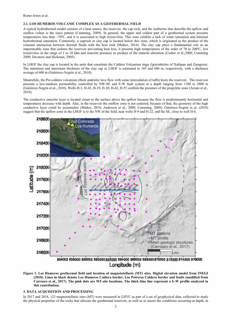
Figure 1. Los Humeros geothermal field and location of magnetotelluric (MT) sites. Digital elevation model from INEGI

(2018). Lines in black denote Los Humeros Caldera border, Los Potreros Caldera border and faults (modified from

Carrasco et al., 2017). The pink dots are MT-site locations. The thick blue line represent a E-W profile analyzed in

this contribution.

3. DATA ACQUISITION AND PROCESSING

In 2017 and 2018, 123 magnetotelluric sites (MT) were measured in LHVC as part of a set of geophysical data, collected to study

the physical properties of the rocks that allocate the geothermal reservoir, as well as to assess the conditions occurring at depth, in

Romo-Jones et al.

3

zones where borehole temperatures larger than 375°C have been observed (Benediktsdóttir et al., 2020). These subjects are part of

GEMex project, an interdisciplinary scientific collaboration (Mexico-European Union) for the assessment of unconventional

geothermal resources.

The MT survey, covers a square area of about 150 km2 and a 25-km-long profile inside LHVC (Figure 1), was designed to

investigate the electrical conductivity distribution to reach about 10 km depth. The natural electromagnetic fields variations in a

frequency band from 0.001 to 1000 Hz were measured with five broadband Metronix instruments. A remote-reference station was

deployed in a site located 78 km away from LHVC, to reduce local noise by using the remote-reference processing technique

(Gamble et al., 1979). In addition, in order to obtain shallow conductivity information for the static shift correction of

magnetotelluric apparent resistivity, 119 transient electromagnetic soundings (TEM) were acquired with a TERRATEM instrument

using a 100 m side single loop array.

We estimate the MT impedance tensor elements (Zxx, Zxy, Zyx, Zyy) with the Bounded Influence Remote Reference Processing

method (BIRRP) proposed by Chave and Thomson (2003, 2004). From the impedance components, the apparent resistivity and

phase curves were estimated for each site, in a period range from 0.001 to 1000 s. The data uncertainty was estimated using the

jackknife procedure proposed by Thomson (1991).

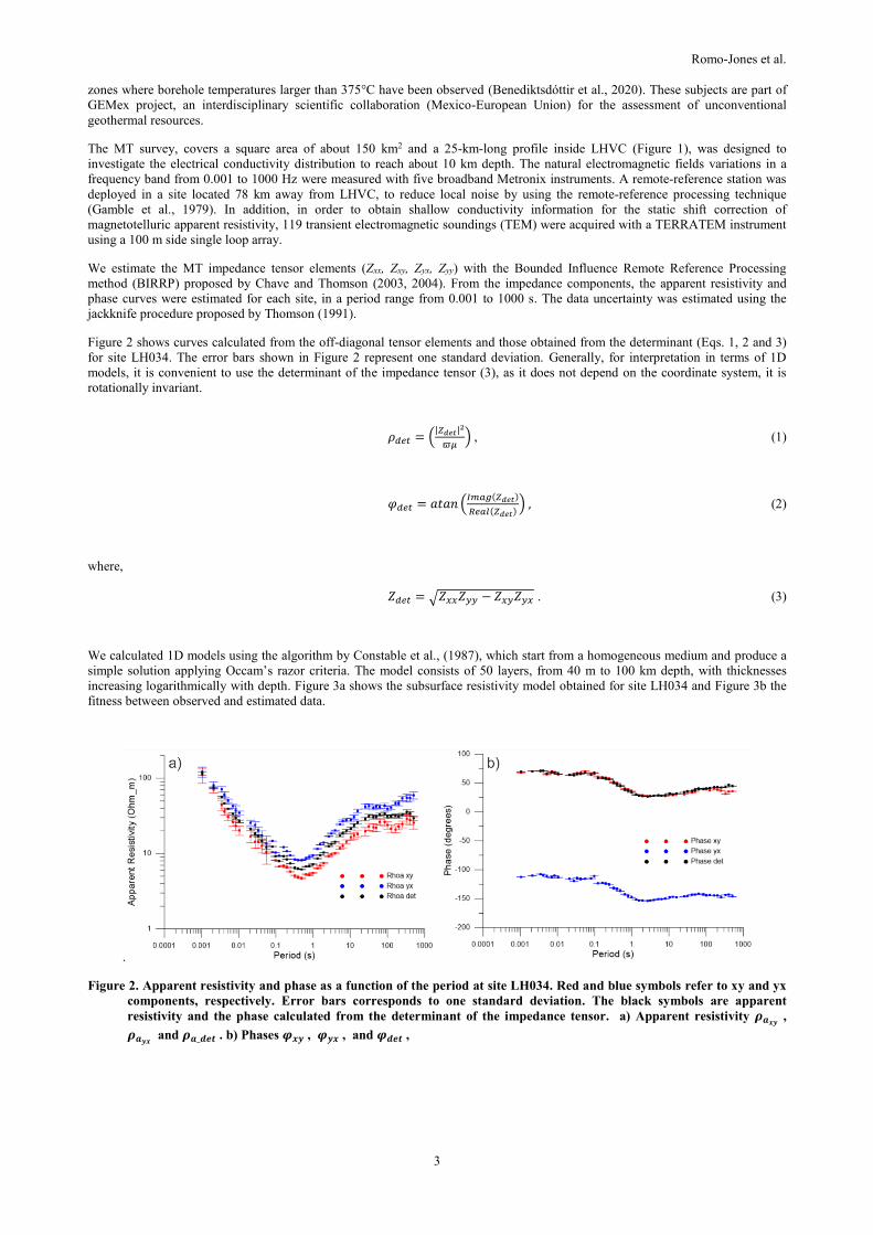
Figure 2 shows curves calculated from the off-diagonal tensor elements and those obtained from the determinant (Eqs. 1, 2 and 3)

for site LH034. The error bars shown in Figure 2 represent one standard deviation. Generally, for interpretation in terms of 1D

models, it is convenient to use the determinant of the impedance tensor (3), as it does not depend on the coordinate system, it is

rotationally invariant.

𝜌𝑑𝑒𝑡 = (|𝑍𝑑𝑒𝑡|2

𝜛𝜇) , (1)

𝜑𝑑𝑒𝑡 = 𝑎𝑡𝑎𝑛 (𝐼𝑚𝑎𝑔(𝑍𝑑𝑒𝑡)

𝑅𝑒𝑎𝑙(𝑍𝑑𝑒𝑡)) , (2)

where,

𝑍𝑑𝑒𝑡 = √𝑍𝑥𝑥𝑍𝑦𝑦 − 𝑍𝑥𝑦𝑍𝑦𝑥 . (3)

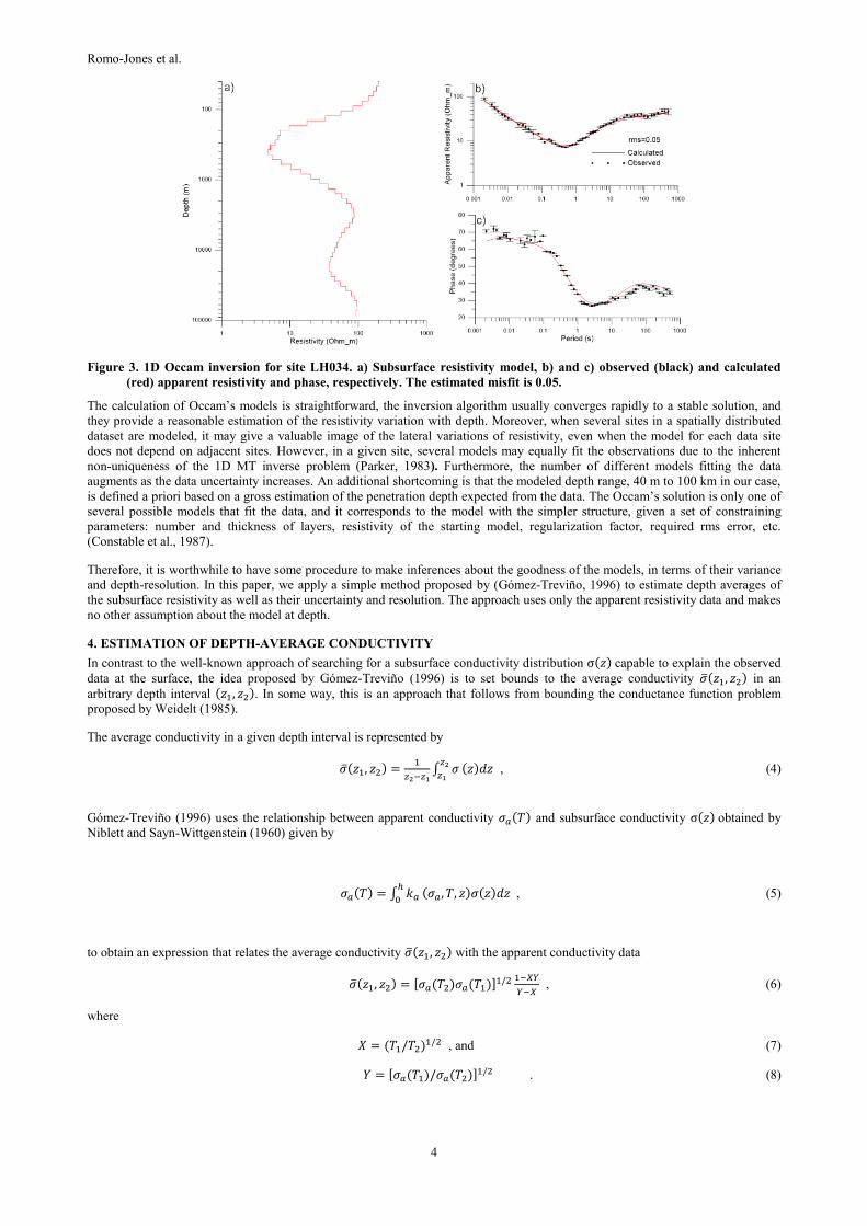
We calculated 1D models using the algorithm by Constable et al., (1987), which start from a homogeneous medium and produce a

simple solution applying Occam’s razor criteria. The model consists of 50 layers, from 40 m to 100 km depth, with thicknesses

increasing logarithmically with depth. Figure 3a shows the subsurface resistivity model obtained for site LH034 and Figure 3b the

fitness between observed and estimated data.

.

Figure 2. Apparent resistivity and phase as a function of the period at site LH034. Red and blue symbols refer to xy and yx

components, respectively. Error bars corresponds to one standard deviation. The black symbols are apparent

resistivity and the phase calculated from the determinant of the impedance tensor. a) Apparent resistivity 𝝆𝒂𝒙𝒚 ,

𝝆𝒂𝒚𝒙 and 𝝆𝒂_𝒅𝒆𝒕 . b) Phases 𝝋𝒙𝒚 , 𝝋𝒚𝒙 , and 𝝋𝒅𝒆𝒕 ,

Romo-Jones et al.

4

Figure 3. 1D Occam inversion for site LH034. a) Subsurface resistivity model, b) and c) observed (black) and calculated

(red) apparent resistivity and phase, respectively. The estimated misfit is 0.05.

The calculation of Occam’s models is straightforward, the inversion algorithm usually converges rapidly to a stable solution, and

they provide a reasonable estimation of the resistivity variation with depth. Moreover, when several sites in a spatially distributed

dataset are modeled, it may give a valuable image of the lateral variations of resistivity, even when the model for each data site

does not depend on adjacent sites. However, in a given site, several models may equally fit the observations due to the inherent

non-uniqueness of the 1D MT inverse problem (Parker, 1983). Furthermore, the number of different models fitting the data

augments as the data uncertainty increases. An additional shortcoming is that the modeled depth range, 40 m to 100 km in our case,

is defined a priori based on a gross estimation of the penetration depth expected from the data. The Occam’s solution is only one of

several possible models that fit the data, and it corresponds to the model with the simpler structure, given a set of constraining

parameters: number and thickness of layers, resistivity of the starting model, regularization factor, required rms error, etc.

(Constable et al., 1987).

Therefore, it is worthwhile to have some procedure to make inferences about the goodness of the models, in terms of their variance

and depth-resolution. In this paper, we apply a simple method proposed by (Gómez-Treviño, 1996) to estimate depth averages of

the subsurface resistivity as well as their uncertainty and resolution. The approach uses only the apparent resistivity data and makes

no other assumption about the model at depth.

4. ESTIMATION OF DEPTH-AVERAGE CONDUCTIVITY

In contrast to the well-known approach of searching for a subsurface conductivity distribution σ(𝑧) capable to explain the observed

data at the surface, the idea proposed by Gómez-Treviño (1996) is to set bounds to the average conductivity (𝑧1, 𝑧2) in an

arbitrary depth interval (𝑧1, 𝑧2). In some way, this is an approach that follows from bounding the conductance function problem

proposed by Weidelt (1985).

The average conductivity in a given depth interval is represented by

(𝑧1, 𝑧2) =1

𝑧2−𝑧1∫ 𝜎

𝑧2

𝑧1(𝑧)𝑑𝑧 , (4)

Gómez-Treviño (1996) uses the relationship between apparent conductivity 𝜎𝑎(𝑇) and subsurface conductivity σ(𝑧) obtained by

Niblett and Sayn-Wittgenstein (1960) given by

𝜎𝑎(𝑇) = ∫ 𝑘𝑎ℎ

0(𝜎𝑎, 𝑇, 𝑧)𝜎(𝑧)𝑑𝑧 , (5)

to obtain an expression that relates the average conductivity (𝑧1, 𝑧2) with the apparent conductivity data

(𝑧1, 𝑧2) = [𝜎𝑎(𝑇2)𝜎𝑎(𝑇1)]1/2 1−𝑋𝑌

𝑌−𝑋 , (6)

where

𝑋 = (𝑇1/𝑇2)1/2 , and (7)

𝑌 = [𝜎𝑎(𝑇1)/𝜎𝑎(𝑇2)]1/2 . (8)

Romo-Jones et al.

5

In this expression σa(T1) and σa(T2) are apparent conductivities observed at periods T1 and T2, respectively, with T2 > T1. Equation

(6) provides an estimation of the subsurface conductivity by using only two observed data. As expected, the smaller the difference

between T1 and T2 is, the better is the depth resolution, but the conductivity accuracy diminishes. In fact, when T2 T1 the

estimation reduces to the Nibblet-Bostick transformation, widely used in the early days of magnetotelluric interpretation (Bostick,

1977; Jones, 1983).

On the other hand, depth can simply be estimated from the data by using the Bostick’s depth estimation

𝑧1 = (𝑇1

2𝜋𝜇𝑜𝜎𝑎(𝑇1))

1/2 and (9)

𝑧2 = (𝑇2

2𝜋𝜇𝑜𝜎𝑎(𝑇2))

1/2 . (10)

Therefore, the average conductivity (𝑧1, 𝑧2) can be assigned to a depth calculated from the geometric average of z1 and z2, i.e.

𝑧 = √𝑧1𝑧2 . (11)

The next step is to have a complete statistical inference of the subsurface conductivity and calculate the standard deviation

𝜕[(𝑧1, 𝑧2)] . This is made by using the traditional propagation error formula

𝜕[(𝑧1, 𝑧2)] = √[𝜕(𝑧1,𝑧2)

𝜕𝜎𝑎(𝑇1)]

2𝑉𝑎𝑟[𝜎𝑎(𝑇1)] + [

𝜕(𝑧1,𝑧2)

𝜕𝜎𝑎(𝑇2)]

2𝑉𝑎𝑟[𝜎𝑎(𝑇2)] , (12)

that depends on the data variance as well as of the derivatives given by

𝜕(𝑧1,𝑧2)

𝜕𝜎𝑎(𝑇1)=

1

2𝑌−2

2𝑋2−𝑋𝑌−1−𝑋𝑌

(1−𝑋𝑌−1)2 (13)

and

𝜕(𝑧1,𝑧2)

𝜕𝜎𝑎(𝑇2)=

1

2

2−𝑋𝑌−1−𝑋𝑌

(1−𝑋𝑌−1)2 . (14)

At this point, it is relevant to mention that 𝜕[(𝑧1, 𝑧2)] will always be bigger than the individual standard deviation of 𝜎𝑎(𝑇1), and

𝜎𝑎(𝑇2). Of course, the larger the data variance is, the larger is the uncertainty of the conductivity average. A more critical issue is

that as the smaller the difference between T1 and T2 is, larger is the standard deviation because the denominator of the derivatives

(Eqs. 13 and 14) increases. At the limit, when T1 = T2, the variance is infinite.

In summary, there is a trade-off between depth resolution and conductivity accuracy; one may improve depth resolution only by

losing accuracy in the conductivity value. On the opposite, if the conductivity accuracy is privileged, then depth resolution will

fade.

5. RESULTS

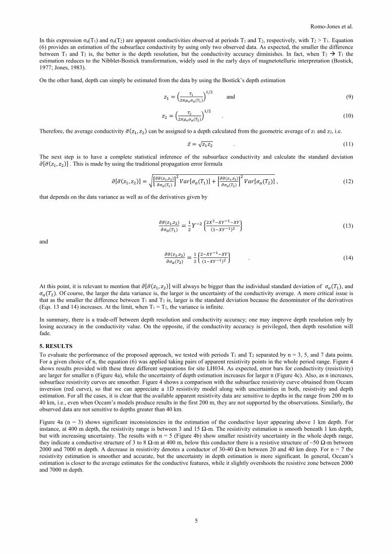
To evaluate the performance of the proposed approach, we tested with periods T1 and T2 separated by n = 3, 5, and 7 data points.

For a given choice of n, the equation (6) was applied taking pairs of apparent resistivity points in the whole period range. Figure 4

shows results provided with these three different separations for site LH034. As expected, error bars for conductivity (resistivity)

are larger for smaller n (Figure 4a), while the uncertainty of depth estimation increases for larger n (Figure 4c). Also, as n increases,

subsurface resistivity curves are smoother. Figure 4 shows a comparison with the subsurface resistivity curve obtained from Occam

inversion (red curve), so that we can appreciate a 1D resistivity model along with uncertainties in both, resistivity and depth

estimation. For all the cases, it is clear that the available apparent resistivity data are sensitive to depths in the range from 200 m to

40 km, i.e., even when Occam’s models produce results in the first 200 m, they are not supported by the observations. Similarly, the

observed data are not sensitive to depths greater than 40 km.

Figure 4a (n = 3) shows significant inconsistencies in the estimation of the conductive layer appearing above 1 km depth. For

instance, at 400 m depth, the resistivity range is between 3 and 15 Ω-m. The resistivity estimation is smooth beneath 1 km depth,

but with increasing uncertainty. The results with n = 5 (Figure 4b) show smaller resistivity uncertainty in the whole depth range,

they indicate a conductive structure of 3 to 8 Ω-m at 400 m, below this conductor there is a resistive structure of ~50 Ω-m between

2000 and 7000 m depth. A decrease in resistivity denotes a conductor of 30-40 Ω-m between 20 and 40 km deep. For n = 7 the

resistivity estimation is smoother and accurate, but the uncertainty in depth estimation is more significant. In general, Occam’s

estimation is closer to the average estimates for the conductive features, while it slightly overshoots the resistive zone between 2000

and 7000 m depth.

Romo-Jones et al.

6

Figure 4. 1D Occam models and average resistivity estimates calculated from equation 6, with three different period

separations, a) n=3, b) n=5, and c) n= 7. Red line is the 1D Occam’s inversion model. Blue symbols are average

resistivity estimations and error bars. The horizontal error bars represent one standard deviation in the resistivity,

and the vertical bars are depth uncertainty estimated from z2 – z1 .

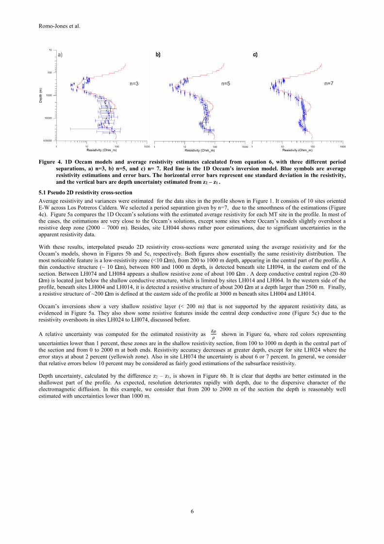
5.1 Pseudo 2D resistivity cross-section

Average resistivity and variances were estimated for the data sites in the profile shown in Figure 1. It consists of 10 sites oriented

E-W across Los Potreros Caldera. We selected a period separation given by n=7, due to the smoothness of the estimations (Figure

4c). Figure 5a compares the 1D Occam’s solutions with the estimated average resistivity for each MT site in the profile. In most of

the cases, the estimations are very close to the Occam’s solutions, except some sites where Occam’s models slightly overshoot a

resistive deep zone (2000 – 7000 m). Besides, site LH044 shows rather poor estimations, due to significant uncertainties in the

apparent resistivity data.

With these results, interpolated pseudo 2D resistivity cross-sections were generated using the average resistivity and for the

Occam’s models, shown in Figures 5b and 5c, respectively. Both figures show essentially the same resistivity distribution. The

most noticeable feature is a low-resistivity zone (<10 Ωm), from 200 to 1000 m depth, appearing in the central part of the profile. A

thin conductive structure (~ 10 Ωm), between 800 and 1000 m depth, is detected beneath site LH094, in the eastern end of the

section. Between LH074 and LH084 appears a shallow resistive zone of about 100 Ωm . A deep conductive central region (20-80

Ωm) is located just below the shallow conductive structure, which is limited by sites LH014 and LH064. In the western side of the

profile, beneath sites LH004 and LH014, it is detected a resistive structure of about 200 Ωm at a depth larger than 2500 m. Finally,

a resistive structure of ~200 Ωm is defined at the eastern side of the profile at 3000 m beneath sites LH004 and LH014.

Occam’s inversions show a very shallow resistive layer (< 200 m) that is not supported by the apparent resistivity data, as

evidenced in Figure 5a. They also show some resistive features inside the central deep conductive zone (Figure 5c) due to the

resistivity overshoots in sites LH024 to LH074, discussed before.

A relative uncertainty was computed for the estimated resistivity as 𝛿𝜌

𝜌 shown in Figure 6a, where red colors representing

uncertainties lower than 1 percent, these zones are in the shallow resistivity section, from 100 to 1000 m depth in the central part of

the section and from 0 to 2000 m at both ends. Resistivity accuracy decreases at greater depth, except for site LH024 where the

error stays at about 2 percent (yellowish zone). Also in site LH074 the uncertainty is about 6 or 7 percent. In general, we consider

that relative errors below 10 percent may be considered as fairly good estimations of the subsurface resistivity.

Depth uncertainty, calculated by the difference z2 – z1, is shown in Figure 6b. It is clear that depths are better estimated in the

shallowest part of the profile. As expected, resolution deteriorates rapidly with depth, due to the dispersive character of the

electromagnetic diffusion. In this example, we consider that from 200 to 2000 m of the section the depth is reasonably well

estimated with uncertainties lower than 1000 m.

Romo-Jones et al.

7

Figure 5. Pseudo 2D resistivity cross-section. a) Red lines are 1D Occam’s inversion models for each MT site, and blue

symbols represent the average resistivity and error bars (one standard deviation) for resistivity and depth, b) section

interpolated from average estimates, and c) section interpolated from 1D Occam’s inversions. Black dots represent

the data used for the interpolation.

Figure 6. a) Relative uncertainty for resistivity (in percent), b) Depth uncertainty calculated as z2 - z1 (in meters). Black dots

represent the data used for the interpolation.

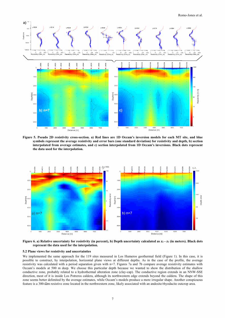
5.2 Plane views for resistivity and uncertainties

We implemented the same approach for the 119 sites measured in Los Humeros geothermal field (Figure 1). In this case, it is

possible to construct, by interpolation, horizontal plane views at different depths. As in the case of the profile, the average

resistivity was calculated with a period separation given with n=7. Figures 7a and 7b compare average resistivity estimates with

Occam’s models at 500 m deep. We choose this particular depth because we wanted to show the distribution of the shallow

conductive zone, probably related to a hydrothermal alteration zone (clay-cap). The conductive region extends in an NNW-SSE

direction, most of it is inside Los Potreros caldera, although its northwestern edge extends beyond the caldera. The shape of this

zone seems better delimited by the average estimates, while Occam’s models produce a more irregular shape. Another conspicuous

feature is a 300-Ωm resistive zone located in the northwestern zone, likely associated with an andesite/rhyodacite outcrop area.

Romo-Jones et al.

8

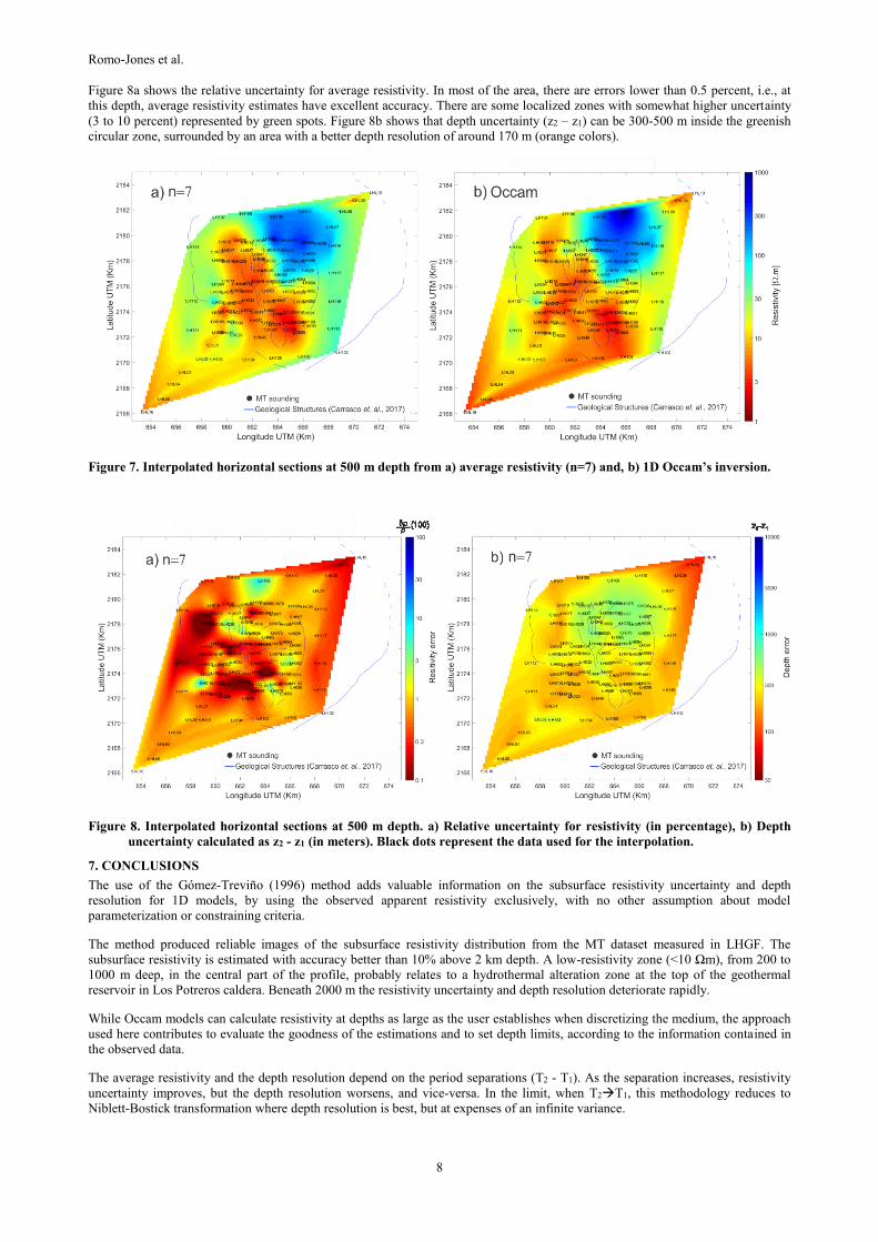
Figure 8a shows the relative uncertainty for average resistivity. In most of the area, there are errors lower than 0.5 percent, i.e., at

this depth, average resistivity estimates have excellent accuracy. There are some localized zones with somewhat higher uncertainty

(3 to 10 percent) represented by green spots. Figure 8b shows that depth uncertainty (z2 – z1) can be 300-500 m inside the greenish

circular zone, surrounded by an area with a better depth resolution of around 170 m (orange colors).

Figure 7. Interpolated horizontal sections at 500 m depth from a) average resistivity (n=7) and, b) 1D Occam’s inversion.

Figure 8. Interpolated horizontal sections at 500 m depth. a) Relative uncertainty for resistivity (in percentage), b) Depth

uncertainty calculated as z2 - z1 (in meters). Black dots represent the data used for the interpolation.

7. CONCLUSIONS

The use of the Gómez-Treviño (1996) method adds valuable information on the subsurface resistivity uncertainty and depth

resolution for 1D models, by using the observed apparent resistivity exclusively, with no other assumption about model

parameterization or constraining criteria.

The method produced reliable images of the subsurface resistivity distribution from the MT dataset measured in LHGF. The

subsurface resistivity is estimated with accuracy better than 10% above 2 km depth. A low-resistivity zone (<10 Ωm), from 200 to

1000 m deep, in the central part of the profile, probably relates to a hydrothermal alteration zone at the top of the geothermal

reservoir in Los Potreros caldera. Beneath 2000 m the resistivity uncertainty and depth resolution deteriorate rapidly.

While Occam models can calculate resistivity at depths as large as the user establishes when discretizing the medium, the approach

used here contributes to evaluate the goodness of the estimations and to set depth limits, according to the information contained in

the observed data.

The average resistivity and the depth resolution depend on the period separations (T2 - T1). As the separation increases, resistivity

uncertainty improves, but the depth resolution worsens, and vice-versa. In the limit, when T2T1, this methodology reduces to

Niblett-Bostick transformation where depth resolution is best, but at expenses of an infinite variance.

Romo-Jones et al.

9

As it is evident in the formulas used here, the calculation of statistical bounds for 1D models is straightforward and may result very

usable to complement information produced by conventional inversion techniques.

ACKNOWLEDGEMENTS

GEMex project is funded by the Mexican Energy Sustainability Fund CONACYT-SENER, Project 2015-04-268074 and by the

European Union’s Horizon 2020 research and innovation programme under grant agreement No. 727550.

REFERENCES

Arzate, J., Corbo-Camargo, F., Carrasco-Núñez, G., Hernández, J., & Yutsis, V. (2018). The Los Humeros (Mexico) geothermal

field model deduced from new geophysical and geological data. Geothermics, 71, 200-211.

Anderson E., Crosby, D. and Ussher, G. (2000), “Bulls-eye! - simple resistivity imaging to reliably locate the geothermal

reservoir,” World Geothermal Congress Proceedings 2000, 909- 914.

Benediktsdóttir, Á., Arango-Galván, C., Hersir, G.P., Held, S., Romo-Jones J.M., Salas-Corrales J.L., Avilés-Esquivel T.A., Ruiz-

Aguilar D., Vilhjálmsson, A.M., Manzella, A., Santilano, A.; The Los Humeros superhot geothermal resource in Mexico:

Resistivity survey (TEM and MT); data acquisition, processing and inversion – geological significance - H2020 GEMex

Project, Proceedings World Geothermal Congress 2020, Reykjavik, Iceland, April 26 – May 2, 2020.

Bostick, F.x., (1977). A simple almost exact method of magnetotelluric analysis, in Workshop on Electrical Methods in Geothermal

Exploration, US Geo. Surv., Contract No. 14080001-G-359.

Chave, A. D., and Thomson, D. J. (2004). Bounded influence magnetotelluric response function estimation. Geophysical Journal

International, 157(3), 988-1006.

Chave, A. D. and Thomson, D. J. (2003). A bounded influence regression estimator based on the statistics of the hat matrix. Journal

of the Royal Statistical Society: Series C (Applied Statistics), 52(3), 307-322.

Carrasco-Núñez, G., Hernández, J., De León, L., Dávila, P., Norini, G., Bernal, J. P., ... & López-Quiroz, P. (2017). Geologic Map

of Los Humeros volcanic complex and geothermal field, eastern Trans-Mexican Volcanic Belt/Mapa geológico del complejo

volcánico Los Humeros y campo geotérmico, sector oriental del Cinturón Volcánico Trans-Mexicano.

Carrasco-Núñez, G., López-Martínez, M., Hernández, J., & Vargas, V. (2017). Subsurface stratigraphy and its correlation with the

surficial geology at Los Humeros geothermal field, eastern Trans-Mexican Volcanic Belt. Geothermics, 67, 1-17.

Constable, S. C., Parker, R. L., & Constable, C. G. (1987). Occam’s inversion: A practical algorithm for generating smooth models

from electromagnetic sounding data. Geophysics, 52(3), 289-300.

Cumming, W. (2009). Geothermal resource conceptual models using surface exploration data. In: Proceedings Thirty-Fourth

Workshop on Geothermal Reservoir Engineering, Stanford University, Stanford, California, February 9-11, 2009.

Davatzes, N. C., and Hickman, S. (2005). Controls on fault-hosted fluid flow: Preliminary results from the Coso Geothermal Field,

CA. Geothermal Resources Council Transactions, 29, 343-348.

Ferriz, H., and Mahood, G. A. (1984). Eruption rates and compositional trends at Los Humeros volcanic center, Puebla,

Mexico. Journal of Geophysical Research: Solid Earth, 89(B10), 8511-8524.

Ferrari, L., Orozco-Esquivel, T., Manea, V., & Manea, M. (2012). The dynamic history of the Trans-Mexican Volcanic Belt and the

Mexico subduction zone. Tectonophysics, 522, 122-149.

Gamble, T. D., Goubau, W. M., & Clarke, J. (1979). Magnetotellurics with a remote magnetic reference. Geophysics, 44(1), 53-68.

Gómez-Treviño, E. (1996). Approximate depth averages of electrical conductivity from surface magnetotelluric data. Geophysical

Journal International, 127(3), 762-772.

Gutiérrez-Negrín, L. C., Izquierdo-Montalvo, G., & Aragón-Aguilar, A. (2010). Review and update of the main features of the Los

Humeros geothermal field, Mexico. In: Proceedings World Geothermal Congress 2010, Bali, Indonesia.

Jones, A.G., (1983). On the equivalence of the Niblett and Bostick transformation in the magnetotelluric method, Geophysical

Journal Internationa., 53, 72-73.

Muñoz, G. (2014). Exploring for geothermal resources with electromagnetic methods. Surveys in geophysics, 35(1), 101-122.

Niblett E.R. and C. Sayn-Wittgenstein (1960). Variation of electrical conductivity with depth by the magnetotelluric method,

Geophysics, 25, 998-1008.

Parker, R. L. (1983). The magnetotelluric inverse problem. Geophysical surveys, 6(1-2), 5-25.

Ussher, G., Harvey, C., Johnstone, R., & Anderson, E. (2000). Understanding the resistivities observed in geothermal systems.

In: Proceedings World Geothermal Congress 2000, Kyushu - Tohoku, Japan, May 28 - June 10.

Thomson, D. J. (1991). Jackknife error estimates for spectra, coherences, and transfer functions, Advances. Spectral Analysis and

Array Processing, 58-113.

Weidelt, P. (1985). Construction of conductance bounds from magnetotelluric impedances. J. Geophys, 57, 191-206.

Yañez, G. C., and García, D. S. (1982). Exploración de la región geotérmica Los Humeros-Las Derrumbadas. Report CFE.