Defocus Map Estimation and Deblurring from a Single Dual-Pixel Image

Shumian Xin1* Neal Wadhwa2 Tianfan Xue2 Jonathan T. Barron2

Pratul P. Srinivasan2 Jiawen Chen3 Ioannis Gkioulekas1 Rahul Garg2

1Carnegie Mellon University 2Google Research 3Adobe Inc.

AbstractWe present a method that takes as input a single dual-

pixel image, and simultaneously estimates the image’s de-focus map—the amount of defocus blur at each pixel—andrecovers an all-in-focus image. Our method is inspired fromrecent works that leverage the dual-pixel sensors availablein many consumer cameras to assist with autofocus, and usethem for recovery of defocus maps or all-in-focus images.These prior works have solved the two recovery problemsindependently of each other, and often require large labeleddatasets for supervised training. By contrast, we show thatit is beneficial to treat these two closely-connected prob-lems simultaneously. To this end, we set up an optimizationproblem that, by carefully modeling the optics of dual-pixelimages, jointly solves both problems. We use data capturedwith a consumer smartphone camera to demonstrate that,after a one-time calibration step, our approach improvesupon prior works for both defocus map estimation and blurremoval, despite being entirely unsupervised.

1. Introduction

Modern DSLR and mirrorless cameras feature large-aperture lenses that allow collecting more light, but also in-troduce defocus blur, meaning that objects in images appearblurred by an amount proportional to their distance fromthe focal plane. A simple way to reduce defocus blur is tostop down, i.e., shrink the aperture. However, this also re-duces the amount of light reaching the sensor, making theimage noisier. Moreover, stopping down is impossible onfixed-aperture cameras, such as those in most smartphones.More sophisticated techniques fall into two categories. Firstare techniques that add extra hardware (e.g., coded aper-tures [46], specialized lenses [47, 15]), and thus are imprac-tical to deploy at large scale or across already available cam-eras. Second are focus stacking techniques [76] that capturemultiple images at different focus distances, and fuse theminto an all-in-focus image. These techniques require longcapture times, and thus are applicable only to static scenes.

Ideally, defocus blur removal should be done using data

*Work primarily done when Shumian Xin was an intern at Google.

Recovered all-in-focus image Recovered defocus map

Input dual pixel images Calibrated blur kernelsLe

ftR

ight

Near

Far

Figure 1: Given left and right dual-pixel (DP) images andcorresponding spatially-varying blur kernels, our methodjointly estimates an all-in-focus image and defocus map.

from a single capture. Unfortunately, in conventional cam-eras, this task is fundamentally ill-posed: a captured imagemay have no high-frequency content because either the la-tent all-in-focus image lacks such frequencies, or they areremoved by defocus blur. Knowing the defocus map, i.e.,the spatially-varying amount of defocus blur, can help sim-plify blur removal. However, determining the defocus mapfrom a single image is closely-related to monocular depthestimation, which is a challenging problem in its own right.Even if the defocus map were known, recovering an all-in-focus image is still an ill-posed problem, as it requireshallucinating the missing high frequency content.

Dual-pixel (DP) sensors are a recent innovation thatmakes it easier to solve both the defocus map estimationand defocus blur removal problems, with data from a sin-gle capture. Camera manufacturers have introduced suchsensors to many DSLR and smartphone cameras to improveautofocus [2, 36]. Each pixel on a DP sensor is split into twohalves, each capturing light from half of the main lens’ aper-ture, yielding two sub-images per exposure (Fig. 1). Thesecan be thought of as a two-sample lightfield [61], and theirsum is equivalent to the image captured by a regular sensor.

2228

Inputs: Calibrated DP blur kernels

All-in-focus imageRendered DP images

Defocus map

MPI representationInputs: Observed DP imagesLeft Intensity channels

Right

Blend

*Conv.

Blend

Blend

OutputsLeft

Right

Loss terms Regularization terms

Alpha channels…

…

Color smoothness prior , Alpha smoothness prior , Entropy priorData loss , Auxiliary data loss

Near

Far

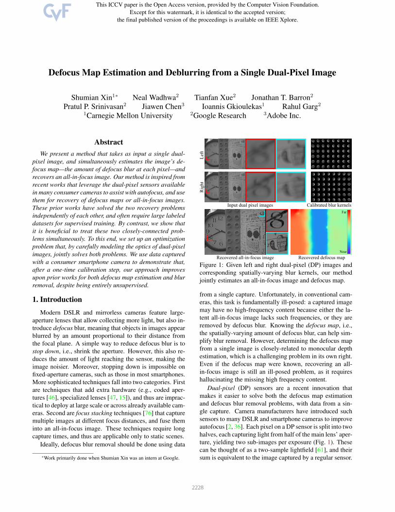
Figure 2: Overview of our proposed method. We use input left and right DP images to fit a multiplane image (MPI) scenerepresentation, consisting of a set of fronto-parallel layers. Each layer is an intensity-alpha image containing the in-focusscene content at the corresponding depth. The MPI can output the all-in-focus image and the defocus map by blending alllayers. It can also render out-of-focus images, by convolving each layer with pre-calibrated blur kernels for the left and rightDP views, and then blending. We optimize the MPI by minimizing a regularized loss comparing rendered and input images.

The two sub-images have different half-aperture-shaped de-focus blur kernels; these are additionally spatially-varyingdue to optical imperfections such as vignetting or field cur-vature in lenses, especially for cheap smartphone lenses.

We propose a method to simultaneously recover the de-focus map and all-in-focus image from a single DP cap-ture. Specifically, we perform a one-time calibration to de-termine the spatially-varying blur kernels for the left andright DP images. Then, given a single DP image, we op-timize a multiplane image (MPI) representation [77, 91] tobest explain the observed DP images using the calibratedblur kernels. An MPI is a layered representation that ac-curately models occlusions, and can be used to render bothdefocused and all-in-focus images, as well as produce a de-focus map. As solving for the MPI from two DP images isunder-constrained, we introduce additional priors and showtheir effectiveness via ablation studies. Further, we showthat in the presence of image noise, standard optimizationhas a bias towards underestimating the amount of defocusblur, and we introduce a bias correction term. Our methoddoes not require large amounts of training data, save fora one-time calibration, and outperforms prior art on bothdefocus map estimation and blur removal, when tested onimages captured using a consumer smartphone camera. Wemake our implementation and data publicly available [85].

2. Related Work

Depth estimation. Multi-view depth estimation is a well-posed and extensively studied problem [30, 71]. By con-trast, single-view, or monocular, depth estimation is ill-posed. Early techniques attempting to recover depth from asingle image typically relied on additional cues, such as sil-houettes, shading, texture, vanishing points, or data-driven

supervision [5, 7, 10, 13, 29, 37, 38, 42, 44, 51, 67, 70, 72].The use of deep neural networks trained on large RGBDdatasets [17, 22, 50, 52, 69, 74] significantly improvedthe performance of data-driven approaches, motivating ap-proaches that use synthetic data [4, 28, 56, 60, 92], self-supervised training [23, 25, 26, 39, 54, 90], or multiple datasources [18, 66]. Despite these advances, producing high-quality depth from a single image remains difficult, due tothe inherent ambiguities of monocular depth estimation.

Recent works have shown that DP data can improvemonocular depth quality, by resolving some of these ambi-guities. Wadhwa et al. [82] applied classical stereo match-ing methods to DP views to compute depth. Punnappurathet al. [64] showed that explicitly modeling defocus blur dur-ing stereo matching can improve depth quality. However,they assume that the defocus blur is spatially invariant andsymmetric between the left and right DP images, which isnot true in real smartphone cameras. Depth estimation withDP images has also been used as part of reflection removalalgorithms [65]. Garg et al. [24] and Zhang et al. [87]trained neural networks to output depth from DP images,using a captured dataset of thousands of DP images andground truth depth maps [3]. The resulting performanceimprovements come at a significant data collection cost.

Focus or defocus has been used as a cue for monoculardepth estimation prior to these DP works. Depth from defo-cus techniques [19, 63, 78, 84] use two differently-focusedimages with the same viewpoint, whereas depth from fo-cus techniques use a dense focal stack [27, 33, 76]. Othermonocular depth estimation techniques use defocus cues assupervision for training depth estimation networks [75], usea coded aperture to estimate depth from one [46, 81, 89]or two captures [88], or estimate a defocus map using syn-

2229

(b) Optics for Lens w/ Aperture (c) Optics for Pinhole Lens

Focal Plane Lens Sensor DP data I

View 1 View 2

Pinhole Sensor

(a) Sensors

I

Dis

pari

ty

o s

Regular Sensor

DP Sensor

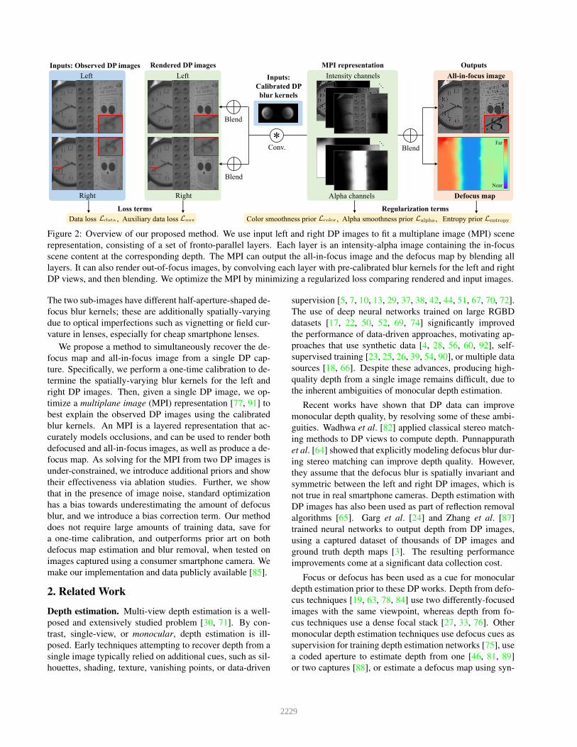
Figure 3: A regular sensor and a DP sensor (a) where eachgreen pixel is split into two halves. For a finite aperturelens (b), an in-focus scene point produces overlapping DPimages, whereas an out-of-focus point produces shifted DPimages. Adding the two DP images yields the image thatwould have been captured by a regular sensor. (c) shows thecorresponding pinhole camera where all scene content is infocus. Ignoring occlusions, images in (b) can be generatedfrom the image in (c) by applying a depth-dependent blur.

thetic data [45]. Lastly, some binocular stereo approachesalso explicitly account for defocus blur [12, 49]; comparedto depth estimation from DP images, these approaches as-sume different focus distances for the two views.Defocus deblurring. Besides depth estimation, measur-ing and removing defocus blur is often desirable to pro-duce sharp all-in-focus images. Defocus deblurring tech-niques usually estimate either a depth map or an equiva-lent defocus map as a first processing stage [14, 40, 62, 73].Some techniques modify the camera hardware to facilitatethis stage. Examples include inserting patterned occlud-ers in the camera aperture to make defocus scale selectioneasier [46, 81, 89, 88]; or sweeping through multiple fo-cal settings within the exposure to make defocus blur spa-tially uniform [59]. Once a defocus map is available, asecond deblurring stage employs non-blind deconvolutionmethods [46, 21, 43, 83, 57, 86] to remove the defocus blur.

Deep learning has been successfully used for defocus de-blurring as well. Lee et al. [45] train neural networks toregress to defocus maps, that are then used to deblur. Abuo-laim and Brown [1] extend this approach to DP data, andtrain a neural network to directly regress from DP imagesto all-in-focus images. Their method relies on a dataset ofpairs of wide and narrow aperture images captured with aDSLR, and may not generalize to images captured on smart-phone cameras, which have very different optical charac-teristics. Such a dataset is impossible to collect on smart-phone cameras with fixed aperture lenses. In contrast tothese prior works, our method does not require difficult-to-capture large datasets. Instead, it uses an accurate model ofthe defocus blur characteristics of DP data, and simultane-ously solves for a defocus map and an all-in-focus image.

3. Dual-Pixel Image FormationWe begin by describing image formation for a regular

and a dual-pixel (DP) sensor, to relate the defocus map and

(a) Left DP image blur kernels (b) Right DP image blur kernels

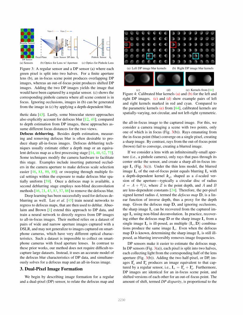
(c) (d) (e) Kernels from [64]Figure 4: Calibrated blur kernels (a) and (b) for the left andright DP images. (c) and (d) show example pairs of leftand right kernels marked in red and cyan. Compared tothe parametric kernels (e) from [64], calibrated kernels arespatially-varying, not circular, and not left-right symmetric.

the all-in-focus image to the captured image. For this, weconsider a camera imaging a scene with two points, onlyone of which is in focus (Fig. 3(b)). Rays emanating fromthe in-focus point (blue) converge on a single pixel, creatinga sharp image. By contrast, rays from the out-of-focus point(brown) fail to converge, creating a blurred image.

If we consider a lens with an infinitesimally-small aper-ture (i.e., a pinhole camera), only rays that pass through itscenter strike the sensor, and create a sharp all-in-focus im-age Is (Fig. 3(c)). Under the thin lens model, the blurredimage Io of the out-of-focus point equals blurring Is witha depth-dependent kernel kd, shaped as a d-scaled ver-sion of the aperture—typically a circular disc of radiusd = A + B/Z, where Z is the point depth, and A and Bare lens-dependent constants [24]. Therefore, the per-pixelsigned kernel radius d, termed the defocus map D, is a lin-ear function of inverse depth, thus a proxy for the depthmap. Given the defocus map D, and ignoring occlusions,the sharp image Is can be recovered from the captured im-age Io using non-blind deconvolution. In practice, recover-ing either the defocus map D or the sharp image Is from asingle image Io is ill-posed, as multiple (Is,D) combina-tions produce the same image Io. Even when the defocusmap D is known, determining the sharp image Is is still ill-posed, as blurring irreversibly removes image frequencies.

DP sensors make it easier to estimate the defocus map.In DP sensors (Fig. 3(a)), each pixel is split into two halves,each collecting light from the corresponding half of the lensaperture (Fig. 3(b)). Adding the two half-pixel, or DP, im-ages Ilo and Iro produces an image equivalent to that cap-tured by a regular sensor, i.e., Io = Ilo + Iro. Furthermore,DP images are identical for an in-focus scene point, andshifted versions of each other for an out-of-focus point. Theamount of shift, termed DP disparity, is proportional to the

2230

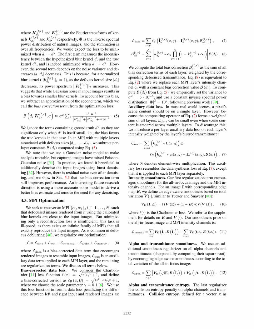
blur size, and thus provides an alternative for defocus mapestimation. In addition to facilitating the estimation of thedefocus map D, having two DP images instead of a singleimage provides additional constraints for recovering the un-derlying sharp image Is. Utilizing these constraints requiresknowing the blur kernel shapes for the two DP images.Blur kernel calibration. As real lenses have spatially-varying kernels, we calibrate an 8 × 6 grid of kernels. Todo this, we fix the focus distance, capture a regular grid ofcircular discs on a monitor screen, and solve for blur ker-nels for left and right images independently using a methodsimilar to Mannan and Langer [55]. When solving for ker-nels, we assume that they are normalized to sum to one, andcalibrate separately for vignetting: we average left and rightimages from six captures of a white diffuser, using the samefocus distance as above, to produce left and right vignettingpatterns Wl and Wr. We refer to the supplement for details.

We show the calibrated blur kernels in Fig. 4. Wenote that these kernels deviate significantly from parametricmodels derived by extending the thin lens model to DP im-age formation [64]. In particular, the calibrated kernels arespatially-varying, not circular, and not symmetric.

4. Proposed MethodThe inputs to our method are two single-channel DP im-

ages, and calibrated left and right blur kernels. We cor-rect for vignetting using Wl and Wr, and denote the twovignetting-corrected DP images as Ilo and Iro, and their cor-responding blur kernels at a certain defocus size d as kl

d andkrd, respectively. We assume that blur kernels at a defocus

size d′ can be obtained by scaling by a factor d′/d [64, 88].

Our goal is to optimize for the multiplane image (MPI) rep-resentation that best explains the observed data, and use it torecover the latent all-in-focus image Is and defocus map D.We first introduce the MPI representation, and show how torender defocused images from it. We then formulate an MPIoptimization problem, and detail its loss function.

4.1. Multiplane Image (MPI) Representation

We model the scene using the MPI representation, previ-ously used primarily for view synthesis [80, 91]. MPIs dis-cretize the 3D space into N fronto-parallel planes at fixeddepths (Fig. 5). We select depths corresponding to linearly-changing defocus blur sizes [d1, . . . , dN ]. Each MPI planeis an intensity-alpha image of the in-focus scene that con-sists of an intensity channel ci and an alpha channel αi.All-in-focus image compositing. Given an MPI, we com-posite the sharp image using the over operator [53]: we sumall layers weighted by the transmittance of each layer ti,

Is =

N∑i=1

tici =

N∑i=1

[ciαi

N∏j=i+1

(1−αj)

]. (1)

Defocused image rendering. Given the left and right blur

*

MPI layers Blur kernels of each layer

All-in-focus image Defocused imageDefocus map

Alpha channels

Defocused MPI layersMPI representation

Intensity channels

Blend Blend Blend

Conv.

Near

Far

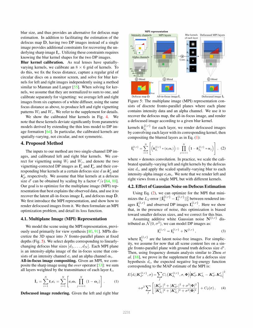
Figure 5: The multiplane image (MPI) representation con-sists of discrete fronto-parallel planes where each planecontains intensity data and an alpha channel. We use it torecover the defocus map, the all-in-focus image, and rendera defocused image according to a given blur kernel.

kernels k{l,r}di

for each layer, we render defocused imagesby convolving each layer with its corresponding kernel, thencompositing the blurred layers as in Eq. (1):

I{l,r}b =

N∑i=1

(k{l,r}di

∗ (ciαi))⊙

N∏j=i+1

(1− k

{l,r}dj

∗αj

) , (2)

where ∗ denotes convolution. In practice, we scale the cali-brated spatially-varying left and right kernels by the defocussize di, and apply the scaled spatially-varying blur to eachintensity-alpha image ciαi. We note that we render left andright views from a single MPI, but with different kernels.

4.2. Effect of Gaussian Noise on Defocus EstimationUsing Eq. (2), we can optimize for the MPI that mini-

mizes the L2-error ||I{l,r}b − I{l,r}o ||22 between rendered im-

ages I{l,r}b and observed DP images I

{l,r}o . Here we show

that, in the presence of noise, this optimization is biasedtoward smaller defocus sizes, and we correct for this bias.

Assuming additive white Gaussian noise N{l,r} dis-tributed as N (0, σ2), we can model DP images as:

I{l,r}o = I{l,r}b +N{l,r} , (3)

where I{l,r}b are the latent noise-free images. For simplic-

ity, we assume for now that all scene content lies on a sin-gle fronto-parallel plane with ground truth defocus size d⋆.Then, using frequency domain analysis similar to Zhou etal. [88], we prove in the supplement that for a defocus sizehypothesis di, the expected negative log-energy functioncorresponding to the MAP estimate of the MPI is:

E(di|K{l,r}

d⋆ , σ)=∑f

C1

(K

{l,r}di

, σ,Φ)∣∣∣Kl

d⋆Krdi −Kr

d⋆Kldi

∣∣∣2+σ2

∑f

[|Kl

d⋆ |2 + |Krd⋆ |2 + σ2|Φ|2

|Kldi|2 + |Kr

di|2 + σ2|Φ|2

]+ C2(σ) , (4)

2231

where K{l,r}di

and K{l,r}d⋆ are the Fourier transforms of ker-

nels k{l,r}di

and k{l,r}d⋆ respectively, Φ is the inverse spectral

power distribution of natural images, and the summation isover all frequencies. We would expect the loss to be mini-mized when di = d⋆. The first term measures the inconsis-tency between the hypothesized blur kernel di and the truekernel d⋆, and is indeed minimized when di = d⋆. How-ever, the second term depends on the noise variance and de-creases as |di| decreases. This is because, for a normalizedblur kernel (||k{l,r}

di||1 = 1), as the defocus kernel size |di|

decreases, its power spectrum ||K{l,r}di

||2 increases. Thissuggests that white Gaussian noise in input images results ina bias towards smaller blur kernels. To account for this bias,we subtract an approximation of the second term, which wecall the bias correction term, from the optimization loss:

B(di|K{l,r}

d⋆ , σ)≈ σ2

∑f

σ2|Φ|2∣∣∣Kldi

∣∣∣2+∣∣∣Krdi

∣∣∣2+σ2|Φ|2. (5)

We ignore the terms containing ground truth d⋆, as they aresignificant only when d⋆ is itself small, i.e., the bias favorsthe true kernels in that case. In an MPI with multiple layersassociated with defocus sizes [d1, . . . , dN ], we subtract per-layer constants B (di) computed using Eq. (5).

We note that we use a Gaussian noise model to makeanalysis tractable, but captured images have mixed Poisson-Gaussian noise [31]. In practice, we found it beneficial toadditionally denoise the input images using burst denois-ing [32]. However, there is residual noise even after denois-ing, and we show in Sec. 5.1 that our bias correction termstill improves performance. An interesting future researchdirection is using a more accurate noise model to derive abetter bias estimate and remove the need for any denoising.

4.3. MPI OptimizationWe seek to recover an MPI {ci,αi} , i ∈ [1, . . . , N ] such

that defocused images rendered from it using the calibratedblur kernels are close to the input images. But minimiz-ing only a reconstruction loss is insufficient: this task isill-posed, as there exists an infinite family of MPIs that allexactly reproduce the input images. As is common in defo-cus deblurring [46], we regularize our optimization:

L = Ldata + Laux + Lintensity + Lalpha + Lentropy , (6)

where Ldata is a bias-corrected data term that encouragesrendered images to resemble input images, Laux is an auxil-iary data term applied to each MPI layer, and the remainingare regularization terms. We discuss all terms below.Bias-corrected data loss. We consider the Charbon-nier [11] loss function ℓ (x) =

√x2/γ2 + 1, and define

a bias-corrected version as ℓB (x,B) =√

(x2−B)/γ2 + 1,where we choose the scale parameter γ = 0.1 [6] . We usethis loss function to form a data loss penalizing the differ-ence between left and right input and rendered images as:

Ldata =∑x,y

ℓB(I{l,r}b (x, y)− I{l,r}o (x, y),B{l,r}

all

), (7)

B{l,r}all =

N∑i=1

[k{l,r}di

∗αi

N∏j=i+1

(1− k

{l,r}dj

∗αj

)]B(di) . (8)

We compute the total bias correction B{l,r}all as the sum of all

bias correction terms of each layer, weighted by the corre-sponding defocused transmittance. Eq. (8) is equivalent toEq. (2) where we replace each MPI layer’s intensity chan-nel ci with a constant bias correction value B (di). To com-pute B (di) from Eq. (5), we empirically set the variance toσ2 = 5 · 10−5, and use a constant inverse spectral powerdistribution |Φ|2 = 102, following previous work [79].Auxiliary data loss. In most real-world scenes, a pixel’sscene content should be on a single layer. However, be-cause the compositing operator of Eq. (2) forms a weightedsum of all layers, Ldata can be small even when scene con-tent is smeared across multiple layers. To discourage this,we introduce a per-layer auxiliary data loss on each layer’sintensity weighted by the layer’s blurred transmittance:

Laux =∑x,y,i

(k{l,r}di

∗ ti(x, y))⊙

ℓB(k{l,r}di

∗ ci(x, y)− I{l,r}o (x, y),B (di)), (9)

where ⊙ denotes element-wise multiplication. This auxil-iary loss resembles the data synthesis loss of Eq. (7), exceptthat it is applied to each MPI layer separately.Intensity smoothness. Our first regularization term encour-ages smoothness for the all-in-focus image and the MPI in-tensity channels. For an image I with corresponding edgemap E, we define an edge-aware smoothness based on totalvariation V (·), similar to Tucker and Snavely [80]:

VE (I,E) = ℓ (V (I)) + (1−E)⊙ ℓ (V (I)) , (10)

where ℓ(·) is the Charbonnier loss. We refer to the supple-ment for details on E and V (·). Our smoothness prior onthe all-in-focus image and MPI intensity channels is:

Lintensity =∑x,y

VE

(Is,E

(Is

))+

∑x,y,i

VE (tici,E (tici)) . (11)

Alpha and transmittance smoothness. We use an ad-ditional smoothness regularizer on all alpha channels andtransmittances (sharpened by computing their square root),by encouraging edge-aware smoothness according to the to-tal variation of the all-in-focus image:

Lalpha =∑x,y,i

[VE

(√αi,E

(Is

))+ VE

(√ti,E

(Is

))]. (12)

Alpha and transmittance entropy. The last regularizeris a collision entropy penalty on alpha channels and trans-mittances. Collision entropy, defined for a vector x as

2232

S (x) = − log ||x||22/||x||21, is a special case of Renyi en-tropy [68], and we empirically found it to be better thanShannon entropy for our problem. Minimizing collision en-tropy encourages sparsity: S (x) is minimum when all butone elements of x are 0, which in our case encourages scenecontent to concentrate on a single MPI layer, rather thanspread across multiple layers. Our entropy loss is:

Lentropy=∑x,y

S([√α2 (x, y) , . . . ,

√αN (x, y)]

T)

+∑x,y

S([√

t1 (x, y) , . . . ,√tN (x, y)

]T). (13)

We extract the alpha channels and transmittances of eachpixel (x, y) from all MPI layers, compute their square rootfor sharpening, compute a per-pixel entropy, and averagethese entropies across all pixels. When computing entropyon alpha channels, we skip the farthest MPI layer, becausewe assume that all scene content ends at the farthest layer,and thus force this layer to be opaque (α1 = 1).

5. Experiments

We capture a new dataset, and use it to perform quali-tative and quantitative comparisons with other state of theart defocus deblurring and defocus map estimation meth-ods. The project website [85] includes an interactive HTMLviewer [8] to facilitate comparisons across our full dataset.Data collection. Even though DP sensors are common, tothe best of our knowledge, only two camera manufactur-ers provide an API to read DP images—Google and Canon.However, Canon’s proprietary software applies an unknownscene-dependent transform to DP data. Unlike supervisedlearning-based methods [1] that can learn to account forthis transform, our loss function requires raw sensor data.Hence, we collect data using the Google Pixel 4 smart-phone, which allows access to the raw DP data [16].

The Pixel 4 captures DP data only in the green chan-nel. To compute ground truth, we capture a focus stackwith 36 slices sampled uniformly in diopter space, wherethe closest focus distance corresponds to the distance wecalibrate for, 13.7 cm, and the farthest to infinity. Follow-ing prior work [64], we use the commercial Helicon Fo-cus software [35] to process the stacks and generate groundtruth sharp images and defocus maps, and we manually cor-rect holes in the generated defocus maps. Still, there areimage regions that are difficult to manually inpaint, e.g.,near occlusion boundaries or curved surfaces. We ignoresuch regions when computing quantitative metrics. We cap-ture a total of 17 scenes, both indoors and outdoors. Simi-lar to Garg et al. [24], we centrally crop the DP images to1008 × 1344. We refer to the supplement for more details.Our dataset is available at the project website [85].

5.1. Results

We evaluate our method on both defocus deblurring anddepth-from-defocus tasks. We use N = 12 MPI layers forall scenes in our dataset. We manually determine the ker-nel sizes of the front and back layers, and evenly distributelayers in diopter space. Each optimization runs for 10,000iterations with Adam [41], and takes 2 hours on an NvidiaTitan RTX GPU. We gradually decrease the global learningrate from 0.3 to 0.1 with exponential decay. Our JAX [9]implementation is available at the project website [85].

We compare to state-of-the-art methods for defocus de-blurring ( DPDNet [1], Wiener deconvolution [79, 88]) anddefocus map estimation (DP stereo matching [82], super-vised learning from DP views [24], DP defocus estima-tion based on kernel symmetry [64], Wiener deconvolu-tion [79, 88], DMENet [45]). For methods that take a singleimage as input, we use the average of the left and right DPimages. We also provide both the original and vignettingcorrected DP images as inputs, and report the best result.We show quantitative results in Tab. 1 and qualitative re-sults in Figs. 6 and 7. For the defocus map, we use theaffine-invariant metrics from Garg et al. [24]. Our methodachieves the best quantitative results on both tasks.Defocus deblurring results. Despite the large amountof blur in the input DP images, our method produces de-blurred results with high-frequency details that are close tothe ground truth (Fig. 6). DPDNet makes large errors as it istrained on Canon data and does not generalize. We improvethe accuracy of DPDNet by providing vignetting correctedimages as input, but its accuracy is still lower than ours.Defocus map estimation results. Our method produces de-focus maps that are closest to the ground truth (Fig. 7), espe-cially on textureless regions, such as the toy and clock in thefirst scene. Similar to [64], depth accuracy near edges canbe improved by guided filtering [34] as shown in Fig. 7(d).Ablation studies. We investigate the effect of each lossfunction term by removing them one at a time. Quantitativeresults are in Tab. 2, and qualitative comparisons in Fig. 8.

Our full pipeline has the best overall performance in re-covering all-in-focus images and defocus maps. Lintensity

and Lalpha strongly affect the smoothness of all-in-focusimages and defocus maps, respectively. Without Lentropy

or Laux, even though recovered all-in-focus images arereasonable, scene content is smeared across multiple MPIlayers, leading to incorrect defocus maps. Finally, with-out the bias correction term B, defocus maps are biasedtowards smaller blur radii, especially in textureless areaswhere noise is more apparent, e.g., the white clock area.Results on Data from Abuolaim and Brown [1]. Eventhough Abuolaim and Brown [1] train their model on datafrom a Canon camera, they also capture Pixel 4 data forqualitative tests. We run our method on their Pixel 4 data,using the calibration from our device, and show that our re-

2233

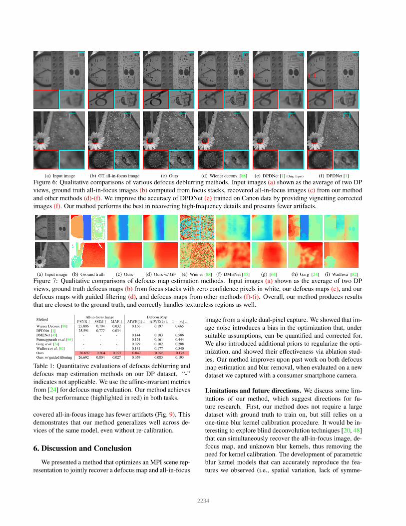
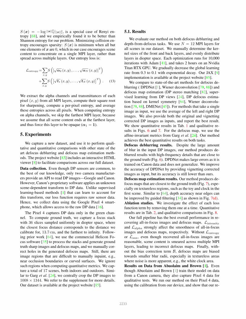
(a) Input image (b) GT all-in-focus image (c) Ours (d) Wiener deconv. [88] (e) DPDNet [1] (Orig. Input) (f) DPDNet [1]Figure 6: Qualitative comparisons of various defocus deblurring methods. Input images (a) shown as the average of two DPviews, ground truth all-in-focus images (b) computed from focus stacks, recovered all-in-focus images (c) from our methodand other methods (d)-(f). We improve the accuracy of DPDNet (e) trained on Canon data by providing vignetting correctedimages (f). Our method performs the best in recovering high-frequency details and presents fewer artifacts.

(a) Input image (b) Ground truth (c) Ours (d) Ours w/ GF (e) Wiener [88] (f) DMENet [45] (g) [64] (h) Garg [24] (i) Wadhwa [82]

Figure 7: Qualitative comparisons of defocus map estimation methods. Input images (a) shown as the average of two DPviews, ground truth defocus maps (b) from focus stacks with zero confidence pixels in white, our defocus maps (c), and ourdefocus maps with guided filtering (d), and defocus maps from other methods (f)-(i). Overall, our method produces resultsthat are closest to the ground truth, and correctly handles textureless regions as well.

Method All-in-focus Image Defocus MapPSNR ↑ SSIM ↑ MAE ↓ AIWE(1) ↓ AIWE(2) ↓ 1− |ρs| ↓

Wiener Deconv. [88] 25.806 0.704 0.032 0.156 0.197 0.665DPDNet [1] 25.591 0.777 0.034 - - -DMENet [45] - - - 0.144 0.183 0.586Punnappurath et al. [64] - - - 0.124 0.161 0.444Garg et al. [24] - - - 0.079 0.102 0.208Wadhwa et al. [82] - - - 0.141 0.177 0.540Ours 26.692 0.804 0.027 0.047 0.076 0.178Ours w/ guided filtering 26.692 0.804 0.027 0.059 0.083 0.193

Table 1: Quantitative evaluations of defocus deblurring anddefocus map estimation methods on our DP dataset. “-”indicates not applicable. We use the affine-invariant metricsfrom [24] for defocus map evaluation. Our method achievesthe best performance (highlighted in red) in both tasks.

covered all-in-focus image has fewer artifacts (Fig. 9). Thisdemonstrates that our method generalizes well across de-vices of the same model, even without re-calibration.

6. Discussion and Conclusion

We presented a method that optimizes an MPI scene rep-resentation to jointly recover a defocus map and all-in-focus

image from a single dual-pixel capture. We showed that im-age noise introduces a bias in the optimization that, undersuitable assumptions, can be quantified and corrected for.We also introduced additional priors to regularize the opti-mization, and showed their effectiveness via ablation stud-ies. Our method improves upon past work on both defocusmap estimation and blur removal, when evaluated on a newdataset we captured with a consumer smartphone camera.

Limitations and future directions. We discuss some lim-itations of our method, which suggest directions for fu-ture research. First, our method does not require a largedataset with ground truth to train on, but still relies on aone-time blur kernel calibration procedure. It would be in-teresting to explore blind deconvolution techniques [20, 48]that can simultaneously recover the all-in-focus image, de-focus map, and unknown blur kernels, thus removing theneed for kernel calibration. The development of parametricblur kernel models that can accurately reproduce the fea-tures we observed (i.e., spatial variation, lack of symme-

2234

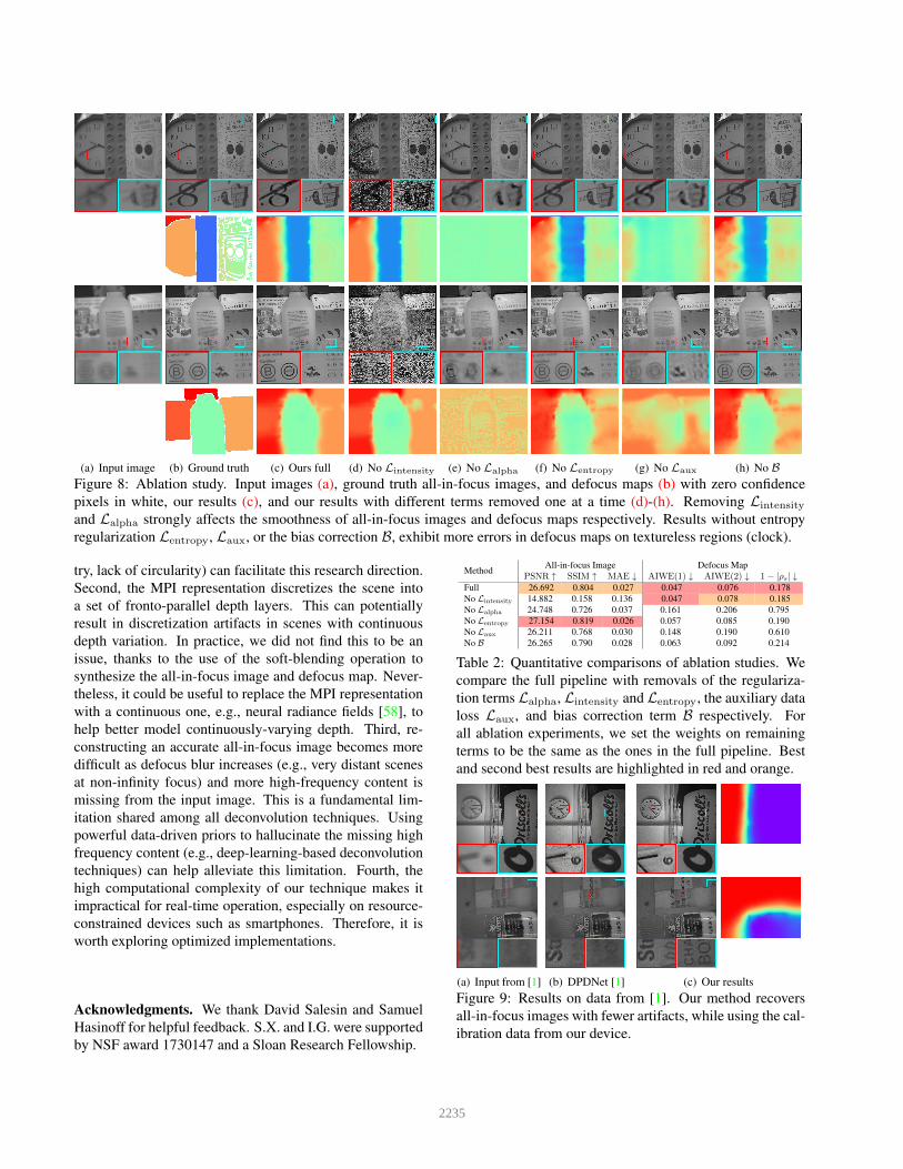
(a) Input image (b) Ground truth (c) Ours full (d) No Lintensity (e) No Lalpha (f) No Lentropy (g) No Laux (h) No BFigure 8: Ablation study. Input images (a), ground truth all-in-focus images, and defocus maps (b) with zero confidencepixels in white, our results (c), and our results with different terms removed one at a time (d)-(h). Removing Lintensity

and Lalpha strongly affects the smoothness of all-in-focus images and defocus maps respectively. Results without entropyregularization Lentropy, Laux, or the bias correction B, exhibit more errors in defocus maps on textureless regions (clock).

try, lack of circularity) can facilitate this research direction.Second, the MPI representation discretizes the scene intoa set of fronto-parallel depth layers. This can potentiallyresult in discretization artifacts in scenes with continuousdepth variation. In practice, we did not find this to be anissue, thanks to the use of the soft-blending operation tosynthesize the all-in-focus image and defocus map. Never-theless, it could be useful to replace the MPI representationwith a continuous one, e.g., neural radiance fields [58], tohelp better model continuously-varying depth. Third, re-constructing an accurate all-in-focus image becomes moredifficult as defocus blur increases (e.g., very distant scenesat non-infinity focus) and more high-frequency content ismissing from the input image. This is a fundamental lim-itation shared among all deconvolution techniques. Usingpowerful data-driven priors to hallucinate the missing highfrequency content (e.g., deep-learning-based deconvolutiontechniques) can help alleviate this limitation. Fourth, thehigh computational complexity of our technique makes itimpractical for real-time operation, especially on resource-constrained devices such as smartphones. Therefore, it isworth exploring optimized implementations.

Acknowledgments. We thank David Salesin and SamuelHasinoff for helpful feedback. S.X. and I.G. were supportedby NSF award 1730147 and a Sloan Research Fellowship.

Method All-in-focus Image Defocus MapPSNR ↑ SSIM ↑ MAE ↓ AIWE(1) ↓ AIWE(2) ↓ 1− |ρs| ↓

Full 26.692 0.804 0.027 0.047 0.076 0.178No Lintensity 14.882 0.158 0.136 0.047 0.078 0.185No Lalpha 24.748 0.726 0.037 0.161 0.206 0.795No Lentropy 27.154 0.819 0.026 0.057 0.085 0.190No Laux 26.211 0.768 0.030 0.148 0.190 0.610No B 26.265 0.790 0.028 0.063 0.092 0.214

Table 2: Quantitative comparisons of ablation studies. Wecompare the full pipeline with removals of the regulariza-tion terms Lalpha, Lintensity and Lentropy, the auxiliary dataloss Laux, and bias correction term B respectively. Forall ablation experiments, we set the weights on remainingterms to be the same as the ones in the full pipeline. Bestand second best results are highlighted in red and orange.

(a) Input from [1] (b) DPDNet [1] (c) Our resultsFigure 9: Results on data from [1]. Our method recoversall-in-focus images with fewer artifacts, while using the cal-ibration data from our device.

2235

References[1] Abdullah Abuolaim and Michael S. Brown. Defocus deblur-

ring using dual-pixel data. European Conference on Com-puter Vision, 2020. 3, 6, 7, 8

[2] Abdullah Abuolaim, Abhijith Punnappurath, and Michael S.Brown. Revisiting autofocus for smartphone cameras. Euro-pean Conference on Computer Vision, 2018. 1

[3] Sameer Ansari, Neal Wadhwa, Rahul Garg, and JiawenChen. Wireless software synchronization of multiple dis-tributed cameras. IEEE International Conference on Com-putational Photography, 2019. 2

[4] Amir Atapour-Abarghouei and Toby P. Breckon. Real-timemonocular depth estimation using synthetic data with do-main adaptation via image style transfer. IEEE/CVF Con-ference on Computer Vision and Pattern Recognition, 2018.2

[5] Ruzena Bajcsy and Lawrence Lieberman. Texture gradientas a depth cue. Computer Graphics and Image Processing,1976. 2

[6] Jonathan T. Barron. A general and adaptive robust loss func-tion. IEEE/CVF Conference on Computer Vision and PatternRecognition, 2019. 5

[7] Jonathan T. Barron and Jitendra Malik. Shape, albedo,and illumination from a single image of an unknown ob-ject. IEEE/CVF Conference on Computer Vision and PatternRecognition, 2012. 2

[8] Benedikt Bitterli, Wenzel Jakob, Jan Novak, and WojciechJarosz. Reversible jump metropolis light transport using in-verse mappings. ACM Transactions on Graphics, 2017. 6

[9] James Bradbury, Roy Frostig, Peter Hawkins,Matthew James Johnson, Chris Leary, Dougal Maclau-rin, George Necula, Adam Paszke, Jake VanderPlas, SkyeWanderman-Milne, and Qiao Zhang. JAX: composabletransformations of Python+NumPy programs, 2018. 6

[10] Michael Brady and Alan Yuille. An extremum principle forshape from contour. IEEE Transactions on Pattern Analysisand Machine Intelligence, 1984. 2

[11] Pierre Charbonnier, Laure Blanc-Feraud, Gilles Aubert, andMichel Barlaud. Two deterministic half-quadratic regular-ization algorithms for computed imaging. IEEE Interna-tional Conference on Image Processing, 1994. 5

[12] Ching-Hui Chen, Hui Zhou, and Timo Ahonen. Blur-awaredisparity estimation from defocus stereo images. IEEE/CVFInternational Conference on Computer Vision, 2015. 3

[13] Sunghwan Choi, Dongbo Min, Bumsub Ham, YoungjungKim, Changjae Oh, and Kwanghoon Sohn. Depth analogy:Data-driven approach for single image depth estimation us-ing gradient samples. IEEE Transactions on Image Process-ing, 2015. 2

[14] Laurent D’Andres, Jordi Salvador, Axel Kochale, and SabineSusstrunk. Non-parametric blur map regression for depth offield extension. IEEE Transactions on Image Processing,2016. 3

[15] Edward R. Dowski and W. Thomas Cathey. Extended depthof field through wave-front coding. Applied optics, 1995. 1

[16] Dual pixel capture app. https://github.com/google-research/google-research/tree/master/dual_pixels. 6

[17] David Eigen, Christian Puhrsch, and Rob Fergus. Depth mapprediction from a single image using a multi-scale deep net-work. Advances in Neural Information Processing Systems,2014. 2

[18] Jose M. Facil, Benjamin Ummenhofer, Huizhong Zhou,Luis Montesano, Thomas Brox, and Javier Civera. Cam-convs: camera-aware multi-scale convolutions for single-view depth. IEEE/CVF Conference on Computer Vision andPattern Recognition, 2019. 2

[19] Paolo Favaro. Recovering thin structures via nonlocal-means regularization with application to depth from defo-cus. IEEE/CVF Conference on Computer Vision and PatternRecognition, 2010. 2

[20] Rob Fergus, Barun Singh, Aaron Hertzmann, Sam T.Roweis, and William T. Freeman. Removing camera shakefrom a single photograph. ACM Transactions on Graphics,2006. 7

[21] D.A. Fish, A.M. Brinicombe, E.R. Pike, and J.G. Walker.Blind deconvolution by means of the Richardson–Lucy al-gorithm. Journal of the Optical Society of America A, 1995.3

[22] Huan Fu, Mingming Gong, Chaohui Wang, Kayhan Bat-manghelich, and Dacheng Tao. Deep ordinal regression net-work for monocular depth estimation. IEEE/CVF Confer-ence on Computer Vision and Pattern Recognition, 2018. 2

[23] Ravi Garg, Vijay Kumar B.G., Gustavo Carneiro, and IanReid. Unsupervised cnn for single view depth estimation:Geometry to the rescue. European Conference on ComputerVision, 2016. 2

[24] Rahul Garg, Neal Wadhwa, Sameer Ansari, and Jonathan T.Barron. Learning single camera depth estimation using dual-pixels. IEEE/CVF International Conference on ComputerVision, 2019. 2, 3, 6, 7

[25] Clement Godard, Oisin Mac Aodha, and Gabriel J. Bros-tow. Unsupervised monocular depth estimation with left-right consistency. IEEE/CVF Conference on Computer Vi-sion and Pattern Recognition, 2017. 2

[26] Clement Godard, Oisin Mac Aodha, and Gabriel J. Bros-tow. Digging into self-supervised monocular depth estima-tion. IEEE/CVF International Conference on Computer Vi-sion, 2019. 2

[27] Paul Grossmann. Depth from focus. Pattern RecognitionLetters, 1987. 2

[28] Xiaoyang Guo, Hongsheng Li, Shuai Yi, Jimmy Ren, andXiaogang Wang. Learning monocular depth by distillingcross-domain stereo networks. European Conference onComputer Vision, 2018. 2

[29] Christian Hane, L’ubor Ladicky, and Marc Pollefeys. Direc-tion matters: Depth estimation with a surface normal classi-fier. IEEE/CVF Conference on Computer Vision and PatternRecognition, 2015. 2

[30] Richard Hartley and Andrew Zisserman. Multiple View Ge-ometry in Computer Vision. Cambridge University Press,2003. 2

2236

[31] Samuel W. Hasinoff, Fredo Durand, and William T. Free-man. Noise-optimal capture for high dynamic range pho-tography. IEEE/CVF Conference on Computer Vision andPattern Recognition, 2010. 5

[32] Samuel W. Hasinoff, Dillon Sharlet, Ryan Geiss, AndrewAdams, Jonathan T. Barron, Florian Kainz, Jiawen Chen, andMarc Levoy. Burst photography for high dynamic range andlow-light imaging on mobile cameras. ACM Transactions onGraphics, 2016. 5

[33] Caner Hazırbas, Sebastian Georg Soyer, Maximilian Chris-tian Staab, Laura Leal-Taixe, and Daniel Cremers. Deepdepth from focus. Asian Conference on Computer Vision,2018. 2

[34] Kaiming He, Jian Sun, and Xiaoou Tang. Guided image fil-tering. European Conference on Computer Vision, 2010. 6

[35] Helicon focus. https://www.heliconsoft.com/. 6[36] Charles Herrmann, Richard Strong Bowen, Neal Wadhwa,

Rahul Garg, Qiurui He, Jonathan T. Barron, and RaminZabih. Learning to autofocus. IEEE/CVF Conference onComputer Vision and Pattern Recognition, 2020. 1

[37] Derek Hoiem, Alexei A. Efros, and Martial Hebert. Auto-matic photo pop-up. ACM Transactions on Graphics, 2005.2

[38] Berthold K.P. Horn. Shape from shading: A method forobtaining the shape of a smooth opaque object from oneview. Technical report, Massachusetts Institute of Technol-ogy, 1970. 2

[39] Huaizu Jiang, Erik G. Learned-Miller, Gustav Larsson,Michael Maire, and Greg Shakhnarovich. Self-superviseddepth learning for urban scene understanding. EuropeanConference on Computer Vision, 2018. 2

[40] Ali Karaali and Claudio Rosito Jung. Edge-based defocusblur estimation with adaptive scale selection. IEEE Transac-tions on Image Processing, 2017. 3

[41] Diederick P. Kingma and Jimmy Ba. Adam: A method forstochastic optimization. International Conference on Learn-ing Representations, 2015. 6

[42] Janusz Konrad, Meng Wang, Prakash Ishwar, Chen Wu, andDebargha Mukherjee. Learning-based, automatic 2d-to-3dimage and video conversion. IEEE Transactions on ImageProcessing, 2013. 2

[43] Dilip Krishnan and Rob Fergus. Fast image deconvolutionusing hyper-laplacian priors. Advances in Neural Informa-tion Processing Systems, 2009. 3

[44] Lubor Ladicky, Jianbo Shi, and Marc Pollefeys. Pullingthings out of perspective. IEEE/CVF Conference on Com-puter Vision and Pattern Recognition, 2014. 2

[45] Junyong Lee, Sungkil Lee, Sunghyun Cho, and SeungyongLee. Deep defocus map estimation using domain adapta-tion. IEEE/CVF Conference on Computer Vision and PatternRecognition, June 2019. 3, 6, 7

[46] Anat Levin, Rob Fergus, Fredo Durand, and William T. Free-man. Image and depth from a conventional camera with acoded aperture. ACM Transactions on Graphics, 2007. 1, 2,3, 5

[47] Anat Levin, Samuel W. Hasinoff, Paul Green, Fredo Durand,and William T. Freeman. 4D frequency analysis of compu-

tational cameras for depth of field extension. ACM Transac-tions on Graphics, 2009. 1

[48] Anat Levin, Yair Weiss, Fredo Durand, and William T. Free-man. Understanding blind deconvolution algorithms. IEEETransactions on Pattern Analysis and Machine Intelligence,2011. 7

[49] Feng Li, Jian Sun, Jue Wang, and Jingyi Yu. Dual-focusstereo imaging. Journal of Electronic Imaging, 2010. 3

[50] Jun Li, Reinhard Klein, and Angela Yao. A two-streamednetwork for estimating fine-scaled depth maps from singlergb images. IEEE/CVF International Conference on Com-puter Vision, 2017. 2

[51] Xiu Li, Hongwei Qin, Yangang Wang, Yongbing Zhang, andQionghai Dai. DEPT: depth estimation by parameter trans-fer for single still images. Asian Conference on ComputerVision, 2014. 2

[52] Fayao Liu, Chunhua Shen, Guosheng Lin, and Ian Reid.Learning depth from single monocular images using deepconvolutional neural fields. IEEE Transactions on PatternAnalysis and Machine Intelligence, 2015. 2

[53] Patric Ljung, Jens Kruger, Eduard Groller, Markus Had-wiger, Charles D. Hansen, and Anders Ynnerman. Stateof the art in transfer functions for direct volume rendering.Computer Graphics Forum, 2016. 4

[54] Reza Mahjourian, Martin Wicke, and Anelia Angelova. Un-supervised learning of depth and ego-motion from monocu-lar video using 3D geometric constraints. IEEE/CVF Con-ference on Computer Vision and Pattern Recognition, 2018.2

[55] Fahim Mannan and Michael S. Langer. Blur calibration fordepth from defocus. Conference on Computer and RobotVision, 2016. 4

[56] Nikolaus Mayer, Eddy Ilg, Philipp Fischer, Caner Hazir-bas, Daniel Cremers, Alexey Dosovitskiy, and Thomas Brox.What makes good synthetic training data for learning dispar-ity and optical flow estimation? International Journal ofComputer Vision, 2018. 2

[57] Tomer Michaeli and Michal Irani. Blind deblurring using in-ternal patch recurrence. European Conference on ComputerVision, 2014. 3

[58] Ben Mildenhall, Pratul P. Srinivasan, Matthew Tancik,Jonathan T. Barron, Ravi Ramamoorthi, and Ren Ng. Nerf:Representing scenes as neural radiance fields for view syn-thesis. European Conference on Computer Vision, 2020. 8

[59] Hajime Nagahara, Sujit Kuthirummal, Changyin Zhou, andShree K. Nayar. Flexible Depth of Field Photography. Euro-pean Conference on Computer Vision, 2008. 3

[60] Jogendra Nath Kundu, Phani Krishna Uppala, Anuj Pahuja,and R. Venkatesh Babu. Adadepth: Unsupervised contentcongruent adaptation for depth estimation. IEEE/CVF Con-ference on Computer Vision and Pattern Recognition, 2018.2

[61] Ren Ng, Marc Levoy, Mathieu Bredif, Gene Duval, MarkHorowitz, and Pat Hanrahan. Light field photography witha hand-held plenoptic camera. Technical report, StanfordUniversity, 2005. 1

2237

[62] Jinsun Park, Yu-Wing Tai, Donghyeon Cho, and InSo Kweon. A unified approach of multi-scale deep and hand-crafted features for defocus estimation. IEEE/CVF Confer-ence on Computer Vision and Pattern Recognition, 2017. 3

[63] Alex Paul Pentland. A new sense for depth of field. IEEETransactions on Pattern Analysis and Machine Intelligence,1987. 2

[64] Abhijith Punnappurath, Abdullah Abuolaim, MahmoudAfifi, and Michael S. Brown. Modeling defocus-disparity indual-pixel sensors. IEEE International Conference on Com-putational Photography, 2020. 2, 3, 4, 6, 7

[65] Abhijith Punnappurath and Michael S. Brown. Reflectionremoval using a dual-pixel sensor. IEEE/CVF Conferenceon Computer Vision and Pattern Recognition, 2019. 2

[66] Rene Ranftl, Katrin Lasinger, David Hafner, KonradSchindler, and Vladlen Koltun. Towards robust monoculardepth estimation: Mixing datasets for zero-shot cross-datasettransfer. IEEE Transactions on Pattern Analysis and Ma-chine Intelligence, 2020. 2

[67] Rene Ranftl, Vibhav Vineet, Qifeng Chen, and VladlenKoltun. Dense monocular depth estimation in complex dy-namic scenes. IEEE/CVF Conference on Computer Visionand Pattern Recognition, 2016. 2

[68] Alfred Renyi. On measures of entropy and information.Berkeley Symposium on Mathematical Statistics and Prob-ability, 1961. 6

[69] Anirban Roy and Sinisa Todorovic. Monocular depth estima-tion using neural regression forest. IEEE/CVF Conference onComputer Vision and Pattern Recognition, 2016. 2

[70] Ashutosh Saxena, Sung H. Chung, and Andrew Y. Ng.Learning depth from single monocular images. Advancesin Neural Information Processing Systems, 2006. 2

[71] Daniel Scharstein and Richard Szeliski. A taxonomy andevaluation of dense two-frame stereo correspondence algo-rithms. International Journal of Computer Vision, 2002. 2

[72] Jianping Shi, Xin Tao, Li Xu, and Jiaya Jia. Break amesroom illusion: depth from general single images. ACMTransactions on Graphics, 2015. 2

[73] Jianping Shi, Li Xu, and Jiaya Jia. Just noticeable defo-cus blur detection and estimation. IEEE/CVF Conferenceon Computer Vision and Pattern Recognition, 2015. 3

[74] Nathan Silberman, Derek Hoiem, Pushmeet Kohli, and RobFergus. Indoor segmentation and support inference fromrgbd images. European Conference on Computer Vision,2012. 2

[75] Pratul P. Srinivasan, Rahul Garg, Neal Wadhwa, Ren Ng,and Jonathan T. Barron. Aperture supervision for monoc-ular depth estimation. IEEE/CVF Conference on ComputerVision and Pattern Recognition, 2018. 2

[76] Supasorn Suwajanakorn, Carlos Hernandez, and Steven M.Seitz. Depth from focus with your mobile phone. IEEE/CVFConference on Computer Vision and Pattern Recognition,2015. 1, 2

[77] Rick Szeliski and Polina Golland. Stereo matching withtransparency and matting. International Journal of Com-puter Vision, 1999. 2

[78] Huixuan Tang, Scott Cohen, Brian Price, Stephen Schiller,and Kiriakos N. Kutulakos. Depth from defocus in thewild. IEEE/CVF Conference on Computer Vision and Pat-tern Recognition, 2017. 2

[79] Huixuan Tang and Kiriakos N. Kutulakos. Utilizing opti-cal aberrations for extended-depth-of-field panoramas. AsianConference on Computer Vision, 2012. 5, 6

[80] Richard Tucker and Noah Snavely. Single-view view syn-thesis with multiplane images. IEEE/CVF Conference onComputer Vision and Pattern Recognition, 2020. 4, 5

[81] Ashok Veeraraghavan, Ramesh Raskar, Amit Agrawal,Ankit Mohan, and Jack Tumblin. Dappled photography:Mask enhanced cameras for heterodyned light fields andcoded aperture refocusing. ACM Transactions on Graphics,2007. 2, 3

[82] Neal Wadhwa, Rahul Garg, David E. Jacobs, Bryan E.Feldman, Nori Kanazawa, Robert Carroll, Yair Movshovitz-Attias, Jonathan T. Barron, Yael Pritch, and Marc Levoy.Synthetic depth-of-field with a single-camera mobile phone.ACM Transactions on Graphics, 2018. 2, 6, 7

[83] Yilun Wang, Junfeng Yang, Wotao Yin, and Yin Zhang. Anew alternating minimization algorithm for total variationimage reconstruction. SIAM Journal on Imaging Sciences,2008. 3

[84] Masahiro Watanabe and Shree K. Nayar. Rational filters forpassive depth from defocus. International Journal of Com-puter Vision, 1998. 2

[85] Shumian Xin, Neal Wadhwa, Tianfan Xue, Jonathan T. Bar-ron, Pratul P. Srinivasan, Jianwen Chen, Ioannis Gkioulekas,and Rahul Garg. Project website, 2021. https://imaging.cs.cmu.edu/dual_pixels. 2, 6

[86] Jiawei Zhang, Jinshan Pan, Wei-Sheng Lai, Rynson W.H.Lau, and Ming-Hsuan Yang. Learning fully convolutionalnetworks for iterative non-blind deconvolution. IEEE/CVFConference on Computer Vision and Pattern Recognition,2017. 3

[87] Yinda Zhang, Neal Wadhwa, Sergio Orts-Escolano, Chris-tian Hane, Sean Fanello, and Rahul Garg. Du2net: Learningdepth estimation from dual-cameras and dual-pixels. Euro-pean Conference on Computer Vision, 2020. 2

[88] Changyin Zhou, Stephen Lin, and Shree K. Nayar. Codedaperture pairs for depth from defocus. IEEE/CVF Interna-tional Conference on Computer Vision, 2009. 2, 3, 4, 6, 7

[89] Changyin Zhou and Shree K. Nayar. What are good aper-tures for defocus deblurring? IEEE International Confer-ence on Computational Photography, 2009. 2, 3

[90] Tinghui Zhou, Matthew Brown, Noah Snavely, and David G.Lowe. Unsupervised learning of depth and ego-motion fromvideo. IEEE/CVF Conference on Computer Vision and Pat-tern Recognition, 2017. 2

[91] Tinghui Zhou, Richard Tucker, John Flynn, Graham Fyffe,and Noah Snavely. Stereo magnification: Learning viewsynthesis using multiplane images. ACM Transactions onGraphics, 2018. 2, 4

[92] Yuliang Zou, Zelun Luo, and Jia-Bin Huang. DF-net: Un-supervised joint learning of depth and flow using cross-taskconsistency. European Conference on Computer Vision,2018. 2

2238