i

Laboratoire des sciences de l'ingénieur, de l'informatique et de l'imagerie

ICube CNRS UMR 7357

École doctorale mathématiques, sciences de l'information et de l'ingénieur

THÈSE

présentée pour obtenir le grade de

Docteur de l'Université de Strasbourg

Mention: Informatique

par

Vasyl Mykhalchuk

Correspondance de maillages dynamiques basée

sur les caractéristiques

Soutenu publiquement le 9 Avril 2015

Members of the jury:

M. Florent Dupont………………………………………………………………………………...Rapporteur

Professeur, Université Claude Bernard Lyon 1, France

M. Hervé Delingette………………………………………………………………….……….…...Rapporteur

Directeur de Recherche, INRIA Sophia-Antipolis, France

M. Edmond Boyer……………………………………………………………………………......Examinateur

Directeur de Recherche, INRIA Grenoble Rhône-Alpes, France

M. Adrian Hilton………………………………………………………..……...………………...Examinateur

Professor , University of Surrey, UK

M. Christian Heinrich………………………………………….……..……...……………..........Examinateur

Professeur, Université de Strasbourg, France

Mme. Hyewon Seo…………………………………………………………………....……Directrice de thèse

CNRS Chargé de recherche, Université de Strasbourg, France

Acknowledgements

ii

Acknowledgements

I wish to express sincere gratitude to my advisors, Hyewon Seo and Frederic Cordier, for their guidance over

the past three years. Their support was invaluable.

Many people have influenced me in this journey. One of the most valuable aspects has been the friendships

I’ve formed within the IGG graphics group. It was a great experience to work with my office mate and col-

league over the years Guoliang Luo. Many thanks to Kenneth Vanhoey and Lionel Untereiner for helping me

to settle down in Strasbourg and sharing their great experience and knowledge. I am also very grateful to

Dominique Bechmann for providing such an enjoyable and stimulating working environment.

I acknowledge Robert Walker Sumner for providing triangle correspondences of the horse and camel mod-

els. I also thank Frederic Larue and Olivier Génevaux for their assistance with the facial motion capture.

A very special thanks to my dearest friends Dima Krasikov and Slava Tarabukhina for brightening every

single day, motivating and uncovering the most important values in life. Finally, I would like to thank my

family for supporting me throughout this process. My mom, my father and my brother Dima provide a foun-

dation in my life on which I know I can always depend.

This work has been supported by the French national project SHARED (Shape Analysis and Registration of

People Using Dynamic Data, No.10-CHEX-014-01).

Strasbourg, le 19 mai 2015

Abstract

iii

Abstract

3D geometry modelling tools and 3D scanners become more enhanced and to a greater degree affordable

today. Thus, development of the new algorithms in geometry processing, shape analysis and shape corre-

spondence gather momentum in computer graphics. Those algorithms steadily extend and increasingly re-

place prevailing methods based on images and videos. Non-rigid shape correspondence or deformable shape

matching has been a long-studied subject in computer graphics and related research fields. Not to forget,

shape correspondence is of wide use in many applications such as statistical shape analysis, motion cloning,

texture transfer, medical applications and many more. However, robust and efficient non-rigid shape corre-

spondence still remains a challenging task due to fundamental variations between individual subjects, acqui-

sition noise and the number of degrees of freedom involved in correspondence search. Although dynamic

2D/3D intra-subject shape correspondence problem has been addressed in the rich set of previous methods,

dynamic inter-subject shape correspondence received much less attention.

The primary purpose of our research is to develop a novel, efficient, robust deforming shape analysis and

correspondence framework for animated meshes based on their dynamic and motion properties. We elabo-

rate our method by exploiting a profitable set of motion data exhibited by deforming meshes with time-

varying embedding. Our approach is based on an observation that a dynamic, deforming shape of a given

subject contains much more information rather than a single static posture of it. That is different from the

existing methods that rely on static shape information for shape correspondence and analysis.

Our framework of deforming shape analysis and correspondence of animated meshes is comprised of several

major contributions: a new dynamic feature detection technique based on multi-scale animated mesh’s de-

formation characteristics, novel dynamic feature descriptor, and an adaptation of a robust graph-based fea-

ture correspondence approach followed by the fine matching of the animated meshes.

First, we present the way to extract valuable inter-frame deformation characteristics from animated mesh’s

surface. Those deformation characteristics effectively capture non-rigid strain deformation values and curva-

ture change of a discrete animated mesh’s surface. We further propose a spatio-temporal multi-scale surface

deformation representation in the animation and a novel spatio-temporal Difference-of-Gaussian feature

detection algorithm. In scope of the work on animated mesh feature detection, a particular emphasis has been

put on robustness and consistency of extracted features. Consequently our method shows robust and consis-

tent feature detection results on animated meshes of drastically different body shapes.

Second, in order to integrate dynamic feature points into a framework for animated mesh correspondence, we

introduce a new dynamic feature descriptor. Motivated by capturing as much as possible of local deforma-

tion and motion properties in the animated mesh, we elaborate a new dynamic feature descriptor composed

of normalized displacement, deformation characteristic curves and Animated Mesh Histogram-of-Gradients.

Given dynamic descriptors for all features on the source and target animations, we further employ a dual

decomposition graph matching approach for establishing reliable feature correspondences between distinct

animated meshes. We demonstrate robustness and effectiveness of dynamic feature matching on a number of

examples.

Abstract

iv

Finally we use dynamic feature correspondences on the source and target to guide an iterative fine matching

of animated meshes in spherical parameterization. Spherical parameterization aids to reduce significantly the

number of degrees of freedom and consequently the computational cost. We demonstrate advantages of our

methods on a range of different animated meshes of varying subjects, movements, complexities and details.

Our correspondence framework is also applicable in the case of animated meshes with time-varying mesh

connectivity. That is possible due to our new efficient landmark transfer algorithm that can be used for inter-

frame matching. The method produces a smooth correspondence map in polynomial time for moderately

non-isometric meshes. To precisely locate any vertex on the source mesh we employ a minimum number

geometric features and their spatial-geodesic relationship. Thus, a mapping of only a small number of feature

points between the source and target meshes allows us to accurately compute arbitrary vertex correspon-

dence. The new developments are demonstrated on a number of examples.

Keywords

Keywords Animated mesh; Feature detection; ·Feature descriptor;· Scale-space theory; Difference of

Gaussians; Shape correspondence

1

Résumé Correspondance de forme est un problème fondamental dans de nombreuses disciplines de recherche, tels

que la géométrie algorithmique, vision par ordinateur et l'infographie. Communément définie comme un

problème de trouver injective/ multivaluée correspondance entre une source et une cible, il constitue une

tâche centrale dans de nombreuses applications y compris le transfert de attributes, récupération des formes

etc. Dans récupération des formes, on peut d'abord calculer la correspondance entre la forme de requête et les

formes dans une base de données, , puis obtenir le meilleure correspondance en utilisant une mesure de

qualité de correspondance prédéfini. Il est également particulièrement avantageuse dans les applications

basées sur la modélisation statistique des formes. En encapsulant les propriétés statistiques de l'anatomie du

sujet dans le model de forme, comme variations géométriques, des variations de densité, etc., il est utile non

seulement pour l'analyse des structures anatomiques telles que des organes ou des os et leur variations

valides, mais aussi pour apprendre les modèle de déformation de la classe d'objets.

Dans cette thèse, nous nous intéressons à une enquête sur une nouvelle méthode d'appariement de forme qui

exploite grande redondance de l'information à partir des ensembles de données dynamiques, variables dans le

temps. Récemment, une grande quantité de recherches ont été effectuées en infographie sur l'établissement

de correspondances entre les mailles statiques (Anguelov, Srinivasan et al. 2005, Aiger, Mitra et al. 2008,

Castellani, Cristani et al. 2008). Ces méthodes reposent sur les caractéristiques géométriques ou les pro-

priétés extrinsèques/intrinsèques des surfaces statiques (Lipman et Funkhouser 2009, Sun, Ovsjanikov et al.

2009, Ovsjanikov, Mérigot et al. 2010, Kim, Lipman et al., 2011) pour élaguer efficacement les paires. Bien

que l'utilisation de la caractéristique géométrique est encore un standard d'or, les méthodes reposant unique-

ment sur l'information statique de formes peuvent générer dans les résultats de correspondance grossièrement

trompeurs lorsque les formes sont radicalement différentes ou ne contiennent pas suffisamment de caractéris-

tiques géométriques.

Nous soutenons qu'en considérant les objets qui subissent une déformation nous pouvons étendre la capacité

limitée des informations de géométrie statique et obtenir correspondences plus fiables et de haute qualité

entre les formes. L'observation clé est qu'un maillage d'animation contient beaucoup plus d'information que

son homologue statique. Fait encourageant, les ensembles de données de maillage animées deviennent plus

populaire et abordable aujourd'hui en raison de l'avancement du développements de capteurs optiques et des

dispositifs de capture de mouvement (Dobrian et Bevilacqua 2003, Vlasic, Adelsberger et al. 2007, Camplani

et Salgado 2012, Webb et Ashley 2012), des performances capture (Valgaerts, Wu et al. 2012, Cao, Weng et

al. 2013), des algorithmes de post-traitement (Weise, Li et al. 2009, Weise, Bouaziz et al., 2011), et des tech-

niques d'animation et reciblage (Sumner et Popović 2004 , Li, Weise et al., 2010).

Intrigué par l'idée d'utiliser des propriétés de déformation dynamique de mailles pour l'amélioration de l'ap-

pariement de formes, nous étudions une nouvelle méthode de correspondance de forme qui tire parti d'un

vaste ensemble d'informations supplémentaires à partir des données de mouvement dynamique des formes.

Comme cela a été discuté, l'emploi des caractéristiques de déformation dynamiques de formes est un inves-

tissement raisonnable qui peut faire une différence significative dans la capacité d'appariement de formes. La

principale contribution que nous apportons dans cette thèse est un nouveau méthode qui traite les caractéris-

tiques de déplacement et de déformation de la surface de sujets - nous élaborons une nouvelle méthode d'ap-

Résumé

2

pariement de formes qui rend l'utilisation de ce riche ensemble d'informations de mouvement qui assure l'ap-

pariement de formes fiable et efficace. Au meilleur de notre connaissance, il n'y a pas de travail existant qui

examine propriétés de déformation ou de mouvement de formes variables dans le temps pour correspon-

dence des forms.

Pour atteindre l'objectif susmentionné, nous nous concentrons sur la façon de représenter efficacement les

données de mouvement et la façon de coder les données de mouvement en vue de trouver une appariement

de formes fiable. Nous reprenons les principales phases d'approches typiques de recherche d'appariement en

incorporant les données dynamiques dans le pipeline de correspondence des formes. Nous développons un

algorithme dynamique d'extraction de caractéristiques multi-échelles, un appariement clairsemé parmi les

caractéristiques en utilisant des signatures de caractéristiques dynamiques, et un fine correspondance de for-

mes. Dans le chapitre 3, nous développons un méthode de détection de caractéristiques spatio-temporel sur

des maillages animés basés sur les approches spatiales à grande échelle. Pour un ensemble donné de carac-

téristiques dynamiques sur chacune des formes source et cible, l'objectif est d'estimer efficacement l'appa-

riement en mettant des points avec signatures similaires de caractéristiques dynamiques en correspondance.

Cette tâche exigeait l'élaboration de mesures de similarité entre des points caractéristiques dynamiques, ce

qui est détaillé au chapitre 4. Les caractéristiques dynamiques ainsi que les caractéristiques géométriques

basé sur la forme sont ensuite utilisés pour guider lappariement dense pour lappariement optimal (chapitre

4).

1.1 Détection de caractéristiques pour les maillages animés

L'extraction de points caractéristiques est un sujet longtemps étudié en vision par ordinateur, traitement de

l'image et l'infographie. Traditionnellement, les caractéristiques sont souvent extraites de différentes modali-

tés et entités graphiques tels que des images 2D / 3D, des vidéos, des maillages polygonaux et des nuages de

points. Par conséquent, il est particulièrement regrettable que le problème de la détection de points caracté-

ristiques sur des maillages animés reste peu étudiée. Bien que les points caractéristiques classiques sont di-

rectement liés à voisinage local statique et à la géométrie, nous proposons une nouvelle technique de détec-

tion de caractéristiques basée sur le comportement dynamique de la forme et de ses caractéristiques de dé-

formation.

Dans cette thèse, nous développons d'abord un cadre de détection de caractéristiques spatio-temporel sur des

maillages animés basés sur les approches spatiales à grande échelle. Notre système de détection de caracté-

ristiques est ensuite utilisée pour la correspondance de forme dynamique clairsemée et dense. Notre algo-

rithme étend les détecteurs spatiales de points d'intérêts sur des maillages statiques (Pauly, Keiser et al. 2003,

Castellani, Cristani et al. 2008, Zaharescu, Boyer et al. 2009, Darom et Keller 2012) de manière à détecter

des points caractéristiques spatio-temporel sur des maillages animés. Basé sur des caractéristiques de défor-

mation calculées à chaque sommet dans chaque trame, nous construisons l'espace d'échelle en calculant dif-

férentes versions lissée des données d'animation. Au cœur de notre algorithme est une nouvelle opérateur

spatio-temporal Différence de Gaussiennes (DoG), ce qui se rapproche de la, Laplace échelle normalisée

spatio-temporelle. En calculant les extrema locaux du nouvel opérateur dans l'espace-temps et de l'échelle,

on obtient des ensembles reproductibles de points caractéristiques spatio-temporelles sur différentes surfaces

déformées modélisées sous forme d'animations de triangle de maillage. Nous validons l'algorithme proposé

dans sa robustesse et la cohérence de détection de caractéristiques. Pour le meilleur de nos connaissances,

notre travail est le premier qui aborde le détection de caractéristiques spatio-temporelle en maillages animés.

Les caractéristique que nous voulons extraire sont les blobs, qui sont situées dans des régions qui présentent

une forte variation de la déformation spatialement et temporellement. Nous définissons d'abord des attributs

de déformation locales sur le maillage d'animation, à partir de laquelle nous construisons une représentation

Résumé

3

multi-échelle de celui-ci. L'une des principales motivations pour fonder notre méthode sur la déformation de

la surface locale peut être expliqué par le fait que (1) la déformation locale sur une surface peut être effica-

cement mesurée par certains principes bien définis, et que (2) la dimension intrinsèque du domaine est de 2D

+ temps (plutôt que 3D + temps) avec une hypothèse raisonnable sur les données.

Nous proposons d'utiliser des tensions de triangle locaux comme une caractéristique de déformation de sur-

face. Par définition tension triangle porte de mesure pure pour de déformation non rigide. Nous améliorer

encore les caractéristiques de déformation par fusion robustesse tension de triangle avec la variation de cour-

bure moyenne. La dernière nous permet de capturer des déformations presque isométriques telles que la

flexion. De telles caractéristiques de déformation, comme nous le montrons dans l'évaluation du procédé,

sont cohérent avec la perception de maillages déformes par l'oeil humain. Deuxièmement, nous aimerions

que le point caractéristique dynamique porte les informations à propos de l'étendue spatiale et temporelle de

la déformation exposée dans un lieu de détection de caractéristiques. En outre, nous avons prouvé être cor-

rect à utiliser des outils mathématiques de la théorie de l'espace échelle linéaire afin de répondre fonctionna-

lité représentation multi-échelle. La théorie de l'espace à l'échelle linéaire est un sous-ensemble des cadres de

l'espace à l'échelle développés dans la communauté de visions par ordinateur dans les années 1980. Au cours

de la dernière décennie, il a attiré l'attention dans l'analyse de surface polygonale. Dans cette thèse, nous

définissons des mécanismes spatiaux à grande échelle pour l'extraction de points caractéristiques de mail-

lages animés. Certains des résultats de détection de caractéristique de notre procédé sont représentées sur la

Figure 1-1.

1.2 Correspondance entre maillages animés

Si nous voulons élaborer des techniques de correspondance de formes, capables d'exploiter des ensembles de

données conséquents sur des images dynamiques, il nous faut mettre en perspective le pipeline traditionnel

des méthodes de correspondance de formes en essayant de comprendre où et comment la mobilité peut être

encapsulée. Pour ce faire, nous nous efforcerons de répondre aux questions suivantes: - Comment représenter

efficacement le mouvement sur des images dynamiques aux différentes étapes de la correspondance de for-

mes? - Comment interpréter les données de mouvement pour trouver des correspondances fiables?

Dans cette thèse nous détaillerons de nouvelles méthodes de correspondances entre différents maillages

animés. Notre méthode se distingue de celles existantes dans son utilisation des propriétés dynamiques des

maillages animés plutôt que dans l'utilisation des ses propriétés géométriques. Dans le cadre de cette thèse

nous avons élaboré un nouveau descripteur de points dynamiques faisant office de signature robuste des

caractéristiques dynamiques. Étant donné la mesure de similarité entres ces descripteurs de points dynami-

ques, nous appréhendons la correspondance de maillages animés en calculant en premier lieu les correspon-

dances des caractéristiques dynamiques puis en établissant ensuite la correspondance complète entre chaque

sommet des animations cibles et des animations sources.

Résumé

4

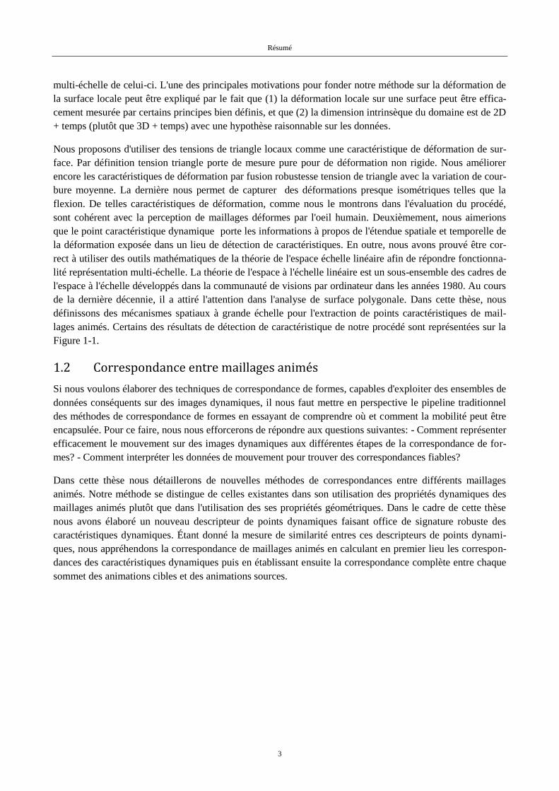
Figure 1-1. points caractéristiques dynamiques détectées par notre cadre sont illustrés sur un certain nombre d'images

sélectionnées de maillages animés. La couleur d'une sphère représente l'échelle temporelle (du bleu au rouge) du point

caractéristique, et le rayon de la sphère indique l'échelle spatiale.

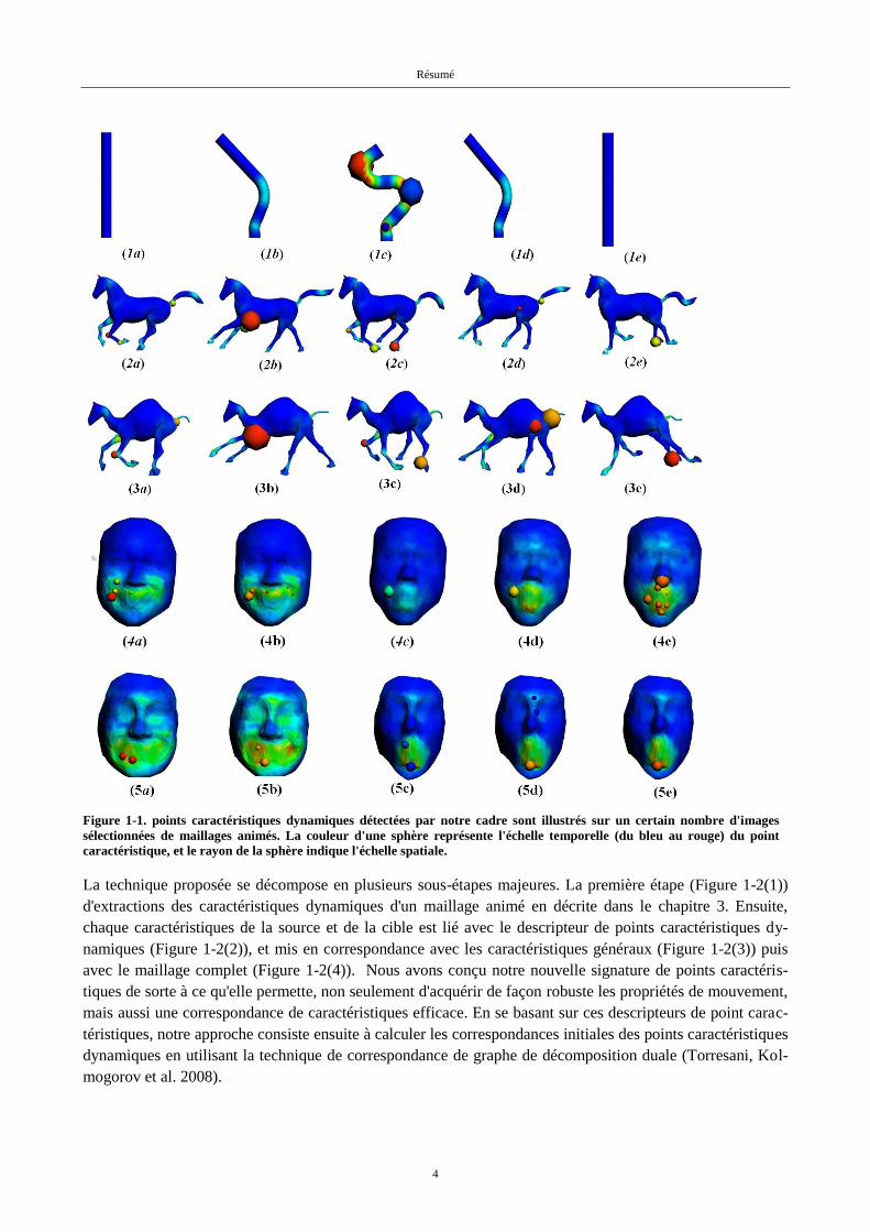
La technique proposée se décompose en plusieurs sous-étapes majeures. La première étape (Figure 1-2(1))

d'extractions des caractéristiques dynamiques d'un maillage animé en décrite dans le chapitre 3. Ensuite,

chaque caractéristiques de la source et de la cible est lié avec le descripteur de points caractéristiques dy-

namiques (Figure 1-2(2)), et mis en correspondance avec les caractéristiques généraux (Figure 1-2(3)) puis

avec le maillage complet (Figure 1-2(4)). Nous avons conçu notre nouvelle signature de points caractéris-

tiques de sorte à ce qu'elle permette, non seulement d'acquérir de façon robuste les propriétés de mouvement,

mais aussi une correspondance de caractéristiques efficace. En se basant sur ces descripteurs de point carac-

téristiques, notre approche consiste ensuite à calculer les correspondances initiales des points caractéristiques

dynamiques en utilisant la technique de correspondance de graphe de décomposition duale (Torresani, Kol-

mogorov et al. 2008).

Résumé

5

Figure 1-2. Pipeline proposée pour établir la correspondance de maillages dynamiques. (1) Détection de caractéristiques

dynamiques. (2) Descripteur de caractéristiques dynamiques. (3) Correspondances des caractéristiques. (4). Correspon-

dance forte.

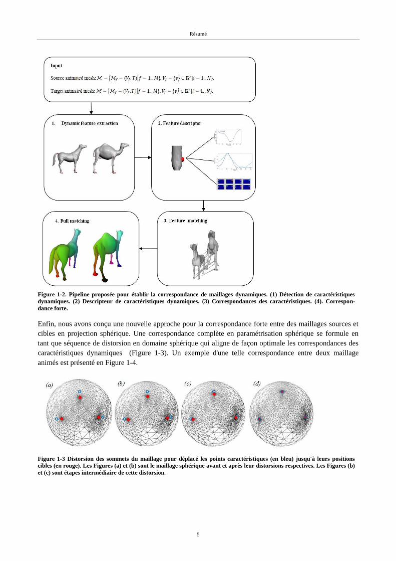
Enfin, nous avons conçu une nouvelle approche pour la correspondance forte entre des maillages sources et

cibles en projection sphérique. Une correspondance complète en paramétrisation sphérique se formule en

tant que séquence de distorsion en domaine sphérique qui aligne de façon optimale les correspondances des

caractéristiques dynamiques (Figure 1-3). Un exemple d'une telle correspondance entre deux maillage

animés est présenté en Figure 1-4.

Figure 1-3 Distorsion des sommets du maillage pour déplacé les points caractéristiques (en bleu) jusqu'à leurs positions

cibles (en rouge). Les Figures (a) et (b) sont le maillage sphérique avant et après leur distorsions respectives. Les Figures (b)

et (c) sont étapes intermédiaire de cette distorsion.

Résumé

6

Figure 1-4. Exemple de correspondance forte. La couleur désigne la correspondance des sommets.

1.3 Cas des maillages animés avec changement de connectivité

Comme établi dans les chapitres 3 et 4, notre framework de détection/description de la caractéristique dy-

namique et la correspondance de la forme basé sur les caractéristiques est conçu pour le domaine des mail-

lages animés. Par définition, un maillage animé est une séquence ordonnée de maillages avec une connec-

tivité de maillage fixée et des correspondances de sommets entre-frames connues au préalable. Cependant,

ceci est une hypothèse relativement forte qui n'est pas nécessairement maintenue pour des grandes variations

de la géométrie dynamique disponible, en particulier, dans la géométrie obtenue par l'acquisition des données

réelles.

Dan le cadre de notre travail, nous abordons le problème du traitement des déformations des maillages qui

changent la connectivité au cours du temps. Nous proposons une technique rapide et efficace, qui peut être

utilisée potentiellement pour établir les correspondances entre-frames dans les maillages qui se déforment au

cours du temps, ce qui lui permet d'être applicable aux algorithmes d'analyse de formes et de correspondance

présentés dans les chapitres 3 et 4.

Notre première observation est que quelques caractéristiques géométriques sont souvent persistantes à

travers les changements et les mouvements des sujets. Ces caractéristiques qui persistent nous permettent de

définir un système de coordonnées géodésiques pour localiser n'importe quel point sur la donnée en entrée et

son correspondant sur le maillage cible. Nous développons notre méthode uniquement pour n'importe quel

sommet indiqué sur la forme, ce qui n'est pas nécessairement significatif géométriquement. L'un des plus

principaux avantages de notre méthode en comparant aux algorithmes de correspondance de forme existants

est son temps de calcul rapide. Ceci est possible car notre méthode est développée de façon optimale pour

utiliser le minimum d'information pour identifier la localisation des points. La méthode a été initialement

développée pour une correspondance rapide et fine et une correspondance grossière de "marqueur". Il est à

Résumé

7

noter que notre méthode de correspondance non rigide est générale et n'est pas limitée uniquement aux corre-

spondances des déformations de maillage entre frame. La méthode peut être utilisée dans plusieurs cas de

correspondance de formes non rigides avec des contraintes isométriques raisonnables. Nous avons montré

une performance robuste de notre méthode pour les correspondances de forme non rigide.

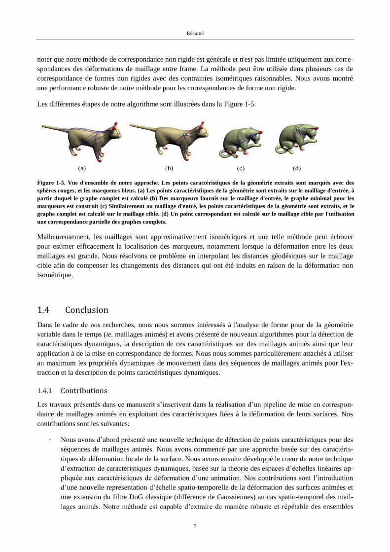
Les différentes étapes de notre algorithme sont illustrées dans la Figure 1-5.

Figure 1-5. Vue d'ensemble de notre approche. Les points caractéristiques de la géométrie extraits sont marqués avec des

sphères rouges, et les marqueurs bleus. (a) Les points caractéristiques de la géométrie sont extraits sur le maillage d'entrée, à

partir duquel le graphe complet est calculé (b) Des marqueurs fournis sur le maillage d'entrée, le graphe minimal pour les

marqueurs est construit (c) Similairement au maillage d'entré, les points caractéristiques de la géométrie sont extraits, et le

graphe complet est calculé sur le maillage cible. (d) Un point correspondant est calculé sur le maillage cible par l'utilisation

une correspondance partielle des graphes complets.

Malheureusement, les maillages sont approximativement isométriques et une telle méthode peut échouer

pour estimer efficacement la localisation des marqueurs, notamment lorsque la déformation entre les deux

maillages est grande. Nous résolvons ce problème en interpolant les distances géodésiques sur le maillage

cible afin de compenser les changements des distances qui ont été induits en raison de la déformation non

isométrique.

1.4 Conclusion

Dans le cadre de nos recherches, nous nous sommes intéressés à l'analyse de forme pour de la géométrie

variable dans le temps (ie. maillages animés) et avons présenté de nouveaux algorithmes pour la détection de

caractéristiques dynamiques, la description de ces caractéristiques sur des maillages animés ainsi que leur

application à de la mise en correspondance de formes. Nous nous sommes particulièrement attachés à utiliser

au maximum les propriétés dynamiques de mouvement dans des séquences de maillages animés pour l'ex-

traction et la description de points caractéristiques dynamiques.

1.4.1 Contributions

Les travaux présentés dans ce manuscrit s’inscrivent dans la réalisation d’un pipeline de mise en correspon-

dance de maillages animés en exploitant des caractéristiques liées à la déformation de leurs surfaces. Nos

contributions sont les suivantes:

∙ Nous avons d’abord présenté une nouvelle technique de détection de points caractéristiques pour des

séquences de maillages animés. Nous avons commencé par une approche basée sur des caractéris-

tiques de déformation locale de la surface. Nous avons ensuite développé le coeur de notre technique

d’extraction de caractéristiques dynamiques, basée sur la théorie des espaces d’échelles linéaires ap-

pliquée aux caractéristiques de déformation d’une animation. Nos contributions sont l’introduction

d’une nouvelle représentation d’échelle spatio-temporelle de la déformation des surfaces animées et

une extension du filtre DoG classique (différence de Gaussiennes) au cas spatio-temporel des mail-

lages animés. Notre méthode est capable d’extraire de manière robuste et répétable des ensembles

Résumé

8

cohérents de points caractéristiques entre les surfaces de différents maillages déformables. Les résul-

tats de nos expérimentations sur différents types de jeux de données montrent une extraction de

points caractéristiques cohérente pour des animations similaires d’un point de vue cinématique et

sémantique.

∙ La principale contribution de nos travaux est un pipeline robuste de mise en correspondance de mail-

lages animés, introduisant un nouveau descripteur de caractéristiques dynamiques. Celui-ci vient

consolider nos nouvelles détection et description de caractéristiques dynamiques, et l’appariement

épar/dense point à point. La nouvelle signature de points dynamiques que nous proposons se com-

pose de différentes modalités de mouvement et propriétés de déformation des maillages animés. Elle

nous a permis de faire un appariement grossier efficace et précis suivi d’un appariement fin robuste

entre différents maillages animés.

∙ Enfin, dans le but de trouver des correspondances inter-frame pour des maillages animés disposant

d’une connectivité évoluant dans le temps, nous avons développé une méthode d’appariement ro-

buste et efficace pour des objets déformables quasi-isométriques. L’idée première est d’utiliser un

minimum d’information pour localiser précisément un point en coordonnées géodésiques sur la sur-

face du maillage source et de reconstruire sa position sur le maillage cible. L’intérêt majeur de la

méthode est le faible coût en temps de calcul de l’appariement, étant donné que seul un nombre de

points réduit a besoin d’être mis en correspondance. Nos tests confirment que cette approche

présente des performances comparables aux algorithmes tirés de l’état de l’art.

1.4.2 Perspectives

Les méthodes étudiées dans ce manuscrit ouvrent la voie à de nouvelles directions prometteuses de recherche

et d’intéressantes applications en rapport avec l’analyse de modèles animées. Voici quelques perspectives

possibles pour ces travaux.

∙ En considérant les développements réalisés dans le cadre de cette thèse, une direction intéressante

serait l’analyse statistique de maillages animés. Une manière de faire serait de mettre au point un

modèle statistique qui capturerait à la fois les variations de la forme et la déformation résultant des

mouvements d’instances distinctes d’animations provenant d’une base de données. De plus, des

méthodes d’apprentissage pourraient être appliquées aux modèles statistiques pour améliorer les

techniques de modélisation et d’animation d’humains virtuels.

∙ Nous envisageons également d’améliorer les algorithmes de mise en correspondance en capturant

davantage de propriétés mécaniques des surfaces déformées. Dans la réalité, les lois de la physique

gouvernent les mouvements et la déformation des objets, ce qui pourrait devenir un composant du

pipeline de mise en correspondance de formes: les propriétés physiques telle que la tension des sur-

faces, ou les directions des tenseurs de déformation (jusqu’à présent nous n’avons employé que les

magnitudes de ces tenseurs) pourraient en effet y être incorporées. Ces propriétés pourraient égale-

ment être introduites dans le descripteur de points caractéristiques dynamiques. Une possibilité serait

d’extraire les propriétés physiques des régions d’intérêt de la source et de comparer les directions du

champ tensoriel de déformation extrait de celles estimées sur le maillage de destination. La mise en

correspondance de formes pourrait alors être exprimée comme une optimisation globale comparant

et alignant les champs tensoriels de déformation des surfaces source et destination.

Enfin, notre détection de points caractéristiques dynamiques peut être employée pour de nombreuses applica-

tions en animation par ordinateur, comme la simplification de surfaces animées, la sélection d’un cadrage

optimal, l’alignement ou la recherche de similarités entre différentes animations.

Résumé

9

∙ Simplifications de surfaces animées. Notre algorithme pourrait être utiliser dans ce but étant donné

qu’il détecte des points caractéristiques se trouvant précisément dans les régions déformées. Leur

échelle spatiale peut être utilisée pour définir des régions dans desquelles le maillage doit conserver

un échantillonnage plus dense lors de la simplification. L’échelle temporelle peut également être

utilisée pour déterminer dynamiquement le coût d’un triangle situé près d’un point caractéristique.

Une très petite échelle temporelle implique une animation soit très courte, soit très rapide, ce qui re-

querrait d’assigner au point caractéristique une priorité basse. À l’inverse, les régions situées autour

de points caractéristiques dotés de grandes échelles temporelles recevraient une priorité plus haute.

∙ Sélection d’un cadrage optimal. Il peut être très commode de disposer d’un outil de sélection auto-

matique de cadrage pour la génération d’aperçus dans des bases de données d’animations. L’idée est

de permettre à l’utilisateur de parcourir l’animation aux points qui maximisent la visibilité des

déformations du maillage. Avec une telle sélection de points de vue, l’utilisateur bénéficie d’une

meilleure perception de l’animation. Une manière tout aussi pratique et simple de sélectionner auto-

matiquement un point de vue optimal est de calculer celui qui maximise le nombre de points carac-

téristiques visibles durant l’optimisation. On peut noter que nos points caractéristiques spatio-

temporels peuvent simplifier la sélection d’un ou de plusieurs bons points de vue. Par exemple, la

qualité d’un point de vue pourrait être définie comme une fonction de la visibilité des ces points

caractéristiques, en termes de nombre total, de variabilité temporelle, de concavité des régions carac-

téristiques projetées (définies par les échelles spatiales et temporelles), etc.

Mots-clés

Keywords Animated mesh; Feature detection; ·Feature descriptor;· Scale-space theory; Difference of

Gaussians; Shape correspondence

10

Contents

Acknowledgements ................................................................................................................................ ii

Abstract ................................................................................................................................................. iii

Keywords ............................................................................................................................................... iv

Résumé ................................................................................................................................................... 1

Mots-clés ................................................................................................................................................. 1

List of notations ................................................................................................................................... 13

List of Figures ...................................................................................................................................... 14

List of Tables ........................................................................................................................................ 18

Chapter 1 Introduction .......................................................................................................... 20

1.1 Context .............................................................................................................................. 20

1.2 Contributions ..................................................................................................................... 22

1.3 List of publications ........................................................................................................... 23

Chapter 2 Related work: Non-rigid correspondence and matching methods ................... 24

2.1 Feature based methods ...................................................................................................... 25

2.2 Tree- or graph- based matching (combinatorial search) ................................................... 25

2.3 Iterative improvement ....................................................................................................... 27

2.4 Voting and clustering ........................................................................................................ 28

2.5 Random sampling ............................................................................................................. 30

2.6 Embedding-based shape correspondence .......................................................................... 31

2.7 Use of prior-knowledge .................................................................................................... 36

Chapter 3 Feature detection for animated meshes .............................................................. 38

3.1 Introduction ....................................................................................................................... 38

3.2 Related work: Feature point detection based on scale-space theory ................................. 40

3.2.1 Feature detection on static meshes ......................................................................... 40

3.2.2 Feature detection on time varying geometry .......................................................... 43

3.3 Animated mesh ................................................................................................................. 45

3.4 Deformation characteristics .............................................................................................. 46

Contents

11

3.5 Basics of linear scale-space theory ................................................................................... 47

3.6 Scale-space of surface deformation characteristics ........................................................... 49

3.6.1 Relationship between box filter and Gaussian filter widths. .................................. 50

3.7 Spatio-temporal DoG operator .......................................................................................... 52

3.8 Feature point detection for animated meshes .................................................................... 53

3.9 Experiments ...................................................................................................................... 55

3.9.1 Consistency ............................................................................................................. 58

3.9.2 Comparison to the manually selected feature points .............................................. 60

3.10 Conclusion ........................................................................................................................ 61

Chapter 4 Correspondence between animated meshes ....................................................... 62

4.1 Introduction ....................................................................................................................... 62

4.2 Related work : Feature point descriptors .......................................................................... 63

4.2.1 Spatial feature descriptors for surface matching ..................................................... 64

4.2.2 Spatio-temporal feature descriptors ........................................................................ 69

4.3 Feature point signature ...................................................................................................... 72

4.3.1 Normalized displacement curves ............................................................................ 73

4.3.2 Spatio-temporal scales ..................................................................................... 75

4.3.3 Deformation characteristics curves ......................................................................... 77

4.3.4 Animated meshes Histogram-of-Gradients (AnimMeshHoG) ............................... 78

4.3.5 Composite descriptor .............................................................................................. 83

4.4 Displacement feature points .............................................................................................. 84

4.5 Feature correspondence via graph matching ..................................................................... 86

4.5.1 Graph matching formulation ................................................................................... 86

4.5.2 Dual decomposition ................................................................................................ 89

4.5.3 Improving geodesic distortion term ........................................................................ 92

4.5.4 Experiments ............................................................................................................ 94

4.6 Full matching .................................................................................................................... 96

4.6.1 Spherical embedding .............................................................................................. 96

4.6.2 Iterative warping ..................................................................................................... 98

4.7 Conclusion ...................................................................................................................... 101

Chapter 5 Case of animated meshes with changing mesh connectivity ........................... 102

5.1 Introduction ..................................................................................................................... 102

5.2 Outline of the method ..................................................................................................... 103

5.3 Graph construction on the source mesh .......................................................................... 104

Contents

12

5.3.1 Geodesic distance computation ............................................................................ 104

5.3.2 Feature point extraction ........................................................................................ 104

5.3.3 Construction of the full graph on the source mesh ............................................... 105

5.3.4 Minimal graph construction .................................................................................. 105

5.4 Landmark transfer via graph matching ........................................................................... 109

5.4.1 Construction of the full graph on the target mesh .......................................... 109

5.4.2 Matching the minimal graph to the full graph ...................................................... 109

5.4.3 Landmark transfer ................................................................................................. 109

5.5 Results ............................................................................................................................. 113

5.5.1 Timing .................................................................................................................. 113

5.5.2 Robustness ............................................................................................................ 114

5.5.3 Inverse distance weighting scheme ...................................................................... 118

5.5.4 Comparison with existing methods ...................................................................... 119

5.5.5 Limitations ............................................................................................................ 120

5.6 Conclusion ...................................................................................................................... 121

Chapter 6 Conclusion ........................................................................................................... 123

6.1 Contributions ................................................................................................................... 123

6.2 Future directions ............................................................................................................. 124

Chapter 7 Appendices .......................................................................................................... 127

7.1 Appendix A. MOCAP Data Acquisition Process ........................................................... 127

7.2 Appendix B : Subgraph matching using Ullmann's Algorithm ...................................... 129

References .......................................................................................................................................... 130

13

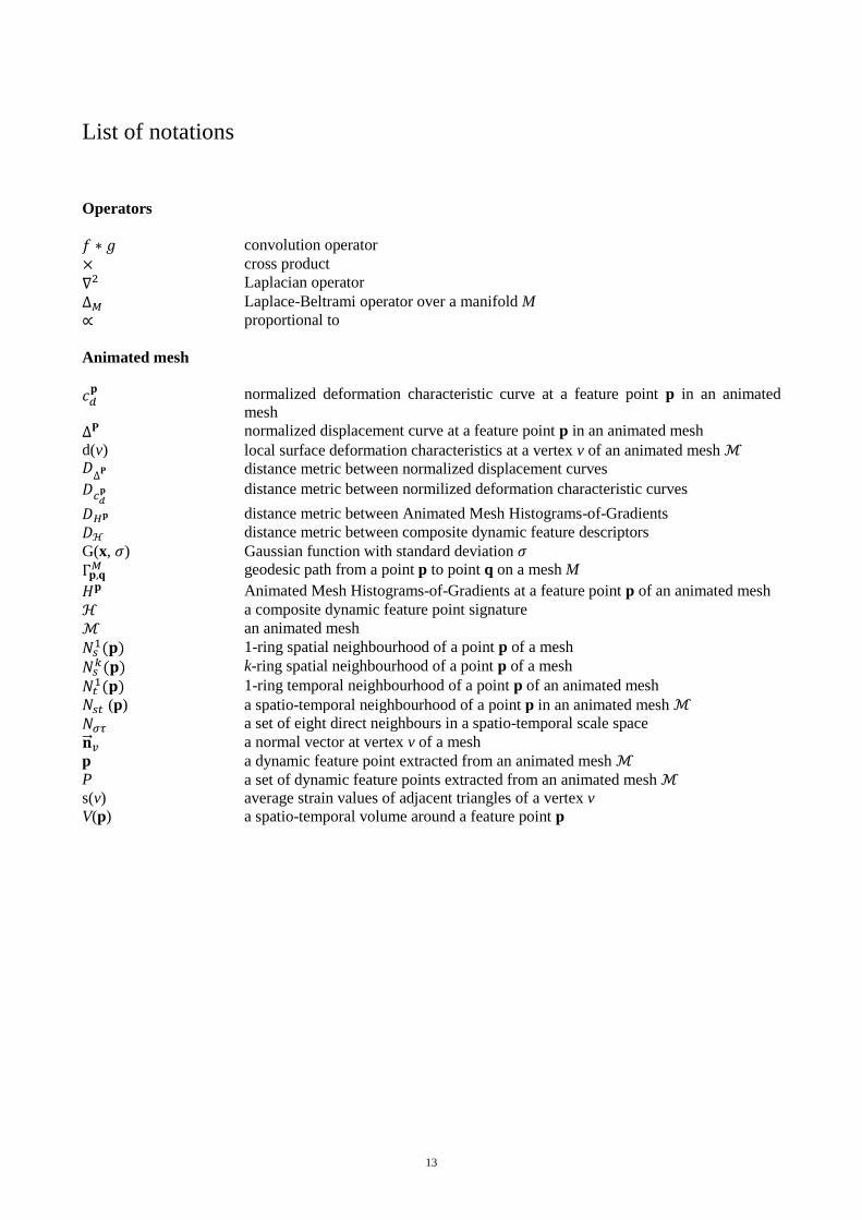
List of notations

Operators

convolution operator

cross product

Laplacian operator

Laplace-Beltrami operator over a manifold M

proportional to

Animated mesh

normalized deformation characteristic curve at a feature point p in an animated

mesh

normalized displacement curve at a feature point p in an animated mesh

d(v) local surface deformation characteristics at a vertex v of an animated mesh

distance metric between normalized displacement curves

distance metric between normilized deformation characteristic curves

distance metric between Animated Mesh Histograms-of-Gradients

distance metric between composite dynamic feature descriptors

G(x, ) Gaussian function with standard deviation

geodesic path from a point p to point q on a mesh M

Animated Mesh Histograms-of-Gradients at a feature point p of an animated mesh

a composite dynamic feature point signature

an animated mesh

1-ring spatial neighbourhood of a point p of a mesh

k-ring spatial neighbourhood of a point p of a mesh

1-ring temporal neighbourhood of a point p of an animated mesh

(p) a spatio-temporal neighbourhood of a point p in an animated mesh

a set of eight direct neighbours in a spatio-temporal scale space

a normal vector at vertex v of a mesh

p a dynamic feature point extracted from an animated mesh

P a set of dynamic feature points extracted from an animated mesh

s(v) average strain values of adjacent triangles of a vertex v

V(p) a spatio-temporal volume around a feature point p

List of Figures

14

List of Figures

Figure 1-1. The overview of the animated mesh correspondence pipeline ............. 21

Figure 2-1. Hierachical matching approach ............................................................ 26

Figure 2-2. Refinement of a hierarchical solution................................................... 26

Figure 2-3. The two-phases deformation of a template via energy minimization ... 28

Figure 2-4. Articulated shape matching .................................................................. 29

Figure 2-5. Electors voting scheme. ........................................................................ 30

Figure 2-6. Matching isometric shapes by embedding them into a lowdimensional

Euclidian space ....................................................................................................... 31

Figure 2-7. Isometric matching with Uniformization of surfaces ........................... 32

Figure 2-8. The pipeline of the Möbius voting algorithm ....................................... 32

Figure 2-9. Blended Intrinsic Maps. ....................................................................... 33

Figure 2-10. Heat Kernel Signature matching ........................................................ 34

Figure 2-11. Heat Kernel Signature correspondence pairs ..................................... 34

Figure 2-12. Matching results between voxelized articulated shapes. .................... 35

Figure 2-13. Alignment of the shapes in spectral domain ....................................... 36

Figure 3-1. Mesh saliency. ...................................................................................... 41

Figure 3-2. Feature detection from photometric scalar field and mean curvature .. 42

Figure 3-3. The neighbourhood of the vertex in scale space of mean curvature .... 42

Figure 3-4. Features computed on armadillo model with Harris operator .............. 43

Figure 3-5. Features on models at different Levels of Details ................................ 43

Figure 3-6. Saliencies based on mean curvature, velocity, and acceleration .......... 44

Figure 3-7.Animated mesh examples ...................................................................... 45

Figure 3-8. Rest shapes for defining the deformation characteristics. .................... 47

Figure 3-9. Local deformation characteristics......................................................... 48

Figure 3-10. The smallest possible spatio-temporal neighborhood ........................ 49

Figure 3-11. Scale space of an input animated mesh. ............................................. 50

Figure 3-12. Multi-scale deformation characteristics on an animated mesh ........... 50

Figure 3-13. The DoG response function evaluation .............................................. 51

Figure 3-14. A 2D illustration of our feature detection method .............................. 54

Figure 3-15. The consistent behavior of our feature detector ................................. 57

Figure 3-16. Dynamic feature points detected by AniM-DoG. ............................... 58

List of Figures

15

Figure 3-17. Inter-subject consistency of feature points ......................................... 59

Figure 3-18. The matching error plots of feature points ......................................... 60

Figure 3-19. Comparison of the manually and automatically selected features ..... 61

Figure 4-1. Proposed pipeline for animated mesh matching. .................................. 63

Figure 4-2. Spin image shape descriptor ................................................................. 64

Figure 4-3. 1-D Curvature maps of Gaussian and Mean curvature......................... 65

Figure 4-4. Illustration of geodesic fans. ................................................................ 65

Figure 4-5. 2D analogy of the Integral Volume descriptor ..................................... 66

Figure 4-6. Clockwise spiral path around a feature point ....................................... 67

Figure 4-7. Spherical histogram used to compute local histograms........................ 67

Figure 4-8. Heat Kernel Signatures for the dragon model ...................................... 68

Figure 4-9. Three isocurves of the Intrinsic wave descriptor .................................. 68

Figure 4-10. IWD descriptor can capture local and global shape properties. ......... 69

Figure 4-11. 2D SIFT image descriptor .................................................................. 69

Figure 4-12. 3D SIFT descriptor ............................................................................. 71

Figure 4-13. The computation pipeline of the HOG3D descriptor. ........................ 71

Figure 4-14. Similarities between drastically different meshes .............................. 72

Figure 4-15.Normalized and not normalized displacement curves. ........................ 74

Figure 4-16. Normalized displacement curves. ....................................................... 74

Figure 4-17. Interpolated displacement curves ....................................................... 75

Figure 4-18. The amplitude of first order normalized derivatives .......................... 76

Figure 4-19. Semantically different features of similar characteristic scales .......... 76

Figure 4-20. Deformation functions of the corresponding features ........................ 78

Figure 4-21. The steps of AnimMeshHoG computation pipeline ........................... 79

Figure 4-22. Consistent normals directions with respect to a feature’s normal ...... 79

Figure 4-23.Spatio-temporal volume centered around dynamic feature ................. 80

Figure 4-24. Scattered deformation characteristics ................................................. 81

Figure 4-25. Deformation characteristics inside spatio-temporal volume. ............. 81

Figure 4-26. Interpolation of AnimMeshHoG histograms ...................................... 82

Figure 4-27. Displacement feature points ............................................................... 85

Figure 4-28.Geodesic distortion in assignments ..................................................... 88

Figure 4-29. Relationship between the primal and dual optimization problems. .... 89

Figure 4-30. Problem decomposition of the dual optimization problem. ............... 90

Figure 4-31. Local subproblem decomposition....................................................... 91

List of Figures

16

Figure 4-32. Average geodesic distance maps. ....................................................... 92

Figure 4-33. Change of average geodesic distance along the paths ........................ 93

Figure 4-34. Edge weights before and after the average geodesic distance prior ... 94

Figure 4-35. Matching result between feature of the cylinders ............................... 95

Figure 4-36. Feature matching result between the horse and camel ....................... 95

Figure 4-37. Inter-subject matching of the dynamic features ................................. 95

Figure 4-38. The bijective mapping using spherical parameterization ................... 97

Figure 4-39. A feature point pair drive the iterative warping steps. ....................... 97

Figure 4-40. Warping of the mesh vertices ............................................................. 98

Figure 4-41. Fine matching between different animated mesh models ................ 100

Figure 5-1. Mesh connectivity is dissimilar in different postures of the subject .. 102

Figure.5-2. Overview of landmark transfer approach ........................................... 103

Figure. 5-3. Convexity and geometric feature points on the mesh........................ 105

Figure. 5-4. Construction of the minimal graph. ................................................... 107

Figure. 5-5. Enclose-by-nodes of the landmark location. ..................................... 107

Figure. 5-6. Influence of pose change on the geodesic path ................................. 110

Figure. 5-7: Histograms of the corresponding point on the source and target ...... 111

Figure. 5-8: The length variation of corresponding geodesic paths ...................... 112

Figure 5-9. The models used have different number mesh structures................... 113

Figure. 5-10. Impact of the landmark location on the quality of transfer ............. 114

Figure 5-11. Results obtained from our landmark transfer technique ................... 115

Figure. 5-12. Quality of landmark transfer with respect to the ground truth ........ 117

Figure. 5-13. Performance of LTMG method on a genus-one plate model .......... 118

Figure. 5-14: Quality of landmark transfer without and with the IDW. .............. 118

Figure. 5-15. Error plots from the BIM, MOB, LTMG techniques ...................... 119

Figure. 5-16. Quality of transferred landmark ...................................................... 122

Figure 7-1. Vicon system installation ................................................................... 127

Figure 7-2. Data aqcuisition in MOCAP session .................................................. 128

17

18

List of Tables

_Toc413763516

Table 3-1. The animated meshes used in the experiments. ..................................... 55

Table 4-1. Time complexity, storage complexity of the feature point signature. ... 84

Table 4-2. Dynamic feature matching results. ........................................................ 94

Table 5-1: Average computation time.of the landmark trasnfer. .......................... 114

19

20

Chapter 2 Introduction

2.1 Context

Shape matching is a fundamental problem in many research disciplines, such as computational geometry, com-

puter vision, and computer graphics. Commonly defined as a problem of finding one-to-one/one-to-

many/many-to-many point-based mappings between a source and a target, it constitutes a central task in nu-

merous applications including attribute transfer, shape retrieval and analysis. For example, it allows an auto-

matic re-usage of attributes, such as texture information or other surface characteristics, from the source object

to a number of targets. In shape retrieval, one can first compute the correspondence between query shape and

the shapes in a database, then obtain the best match by using some predefined matching quality metric. It is also

particularly advantageous in applications based on statistical shape modeling. By encapsulating the statistical

properties of the anatomy of the subject in the shape model, such as inter- and intra-subject geometrical varia-

tions, density variations etc., it is helpful not only for the analysis of anatomical structures such as organs or

bones and their valid variations, but also for learning the deformation models of the given class of objects.

However, finding a reliable, efficient matching is an inherently challenging task, at least due to two reasons:

First, typically large size of data sets increases combinatorially the time complexity of the matching algorithms.

Given two shapes discretized as polygonal meshes of M and N vertices respectively, the exhaustive (brute

force) search for point-to-point correspondence is comprised of

=

evaluations. In order to avoid

impractically expensive brute force search, heuristics are often used for computing the shape correspondence.

Note, that size of time-varying data sets we consider in this dissertation is even higher, which makes it even

more difficult to work with. In this thesis, we first extract feature points using dynamic properties of the ani-

mated mesh, and solve for a sparse matching among the feature points. We then propagate the matching results

to a full matching so that the similarity of dynamic properties is locally maximized. Second difficulty of shape

matching comes from the input data, which can be incomplete or glutted with geometric/topological noise.

Therefore, in order to keep a realistic trade of between the two main shape matching complexities, in this thesis

we focus on processed data sets in a form of animated meshes with a fixed mesh connectivity over time, rather

than directly working on a raw data.

In this thesis, we are interested in investigating a novel shape matching method that exploits large redundancy

of information from dynamic, time-varying datasets. Recently, a large amount of research has been done in

computer graphics on establishing correspondences between static meshes (Anguelov, Srinivasan et al. 2005,

Aiger, Mitra et al. 2008, Castellani, Cristani et al. 2008). These methods rely on the geometric features or ex-

trinsic/intrinsic properties of static surfaces (Lipman and Funkhouser 2009, Sun, Ovsjanikov et al. 2009,

Ovsjanikov, Mérigot et al. 2010, Kim, Lipman et al. 2011) to efficiently prune matching pairs. Although the

use of geometric feature is still a golden standard, methods relying solely on the static information of shapes

can generate in grossly misleading correspondence results when the shapes are drastically different or do not

contain enough geometric features.

We argue that by considering objects that undergo deformation we can extend the limited capability of static

geometry information and obtain more reliable, high quality correspondence computation between shapes. The

21

key observation is that an animated mesh contains significantly more information rather than its static counter-

part. Encouragingly, animated mesh data sets become more popular and affordable today due to advancing

developments of optical sensors and motion capture devices (Dobrian and Bevilacqua 2003, Vlasic,

Adelsberger et al. 2007, Camplani and Salgado 2012, Webb and Ashley 2012), performance capture

schemes(Valgaerts, Wu et al. 2012, Cao, Weng et al. 2013), post processing algorithms (Weise, Li et al. 2009,

Weise, Bouaziz et al. 2011), and animation techniques and retargeting (Sumner and Popović 2004, Li, Weise et

al. 2010).

Intrigued by the idea of using dynamic deformation properties of meshes for the improved shape matching, we

investigate a novel shape correspondence method that takes advantage of a large set of supplementary infor-

mation from shape’s dynamic motion data. As have discussed, employment of shape’s dynamic deformation

characteristics is a reasonable investment that can make a significant difference in the capability of shape corre-

spondence. The main contribution we bring in this thesis is a novel scheme that processes subjects’ movement

and surface deformation characteristics – we devise a new shape matching method that makes use of this rich

bundle of motion information that ensures reliable and efficient shape correspondence. To the best of our

knowledge, there is no existing work that examines deformation or motion properties of time-varying shapes in

shape matching, despite their increasing availability and relevance.

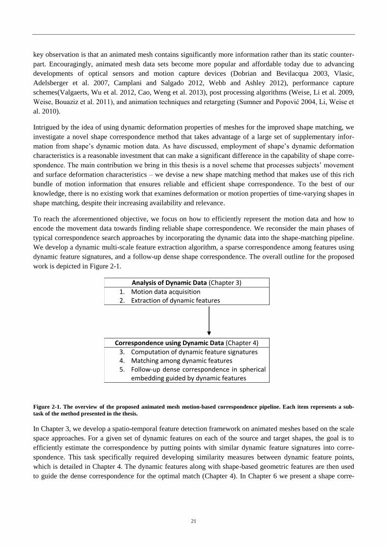
To reach the aforementioned objective, we focus on how to efficiently represent the motion data and how to

encode the movement data towards finding reliable shape correspondence. We reconsider the main phases of

typical correspondence search approaches by incorporating the dynamic data into the shape-matching pipeline.

We develop a dynamic multi-scale feature extraction algorithm, a sparse correspondence among features using

dynamic feature signatures, and a follow-up dense shape correspondence. The overall outline for the proposed

work is depicted in Figure 2-1.

Analysis of Dynamic Data (Chapter 3)

1. Motion data acquisition 2. Extraction of dynamic features

Correspondence using Dynamic Data (Chapter 4)

3. Computation of dynamic feature signatures 4. Matching among dynamic features 5. Follow-up dense correspondence in spherical

embedding guided by dynamic features

Figure 2-1. The overview of the proposed animated mesh motion-based correspondence pipeline. Each item represents a sub-

task of the method presented in the thesis.

In Chapter 3, we develop a spatio-temporal feature detection framework on animated meshes based on the scale

space approaches. For a given set of dynamic features on each of the source and target shapes, the goal is to

efficiently estimate the correspondence by putting points with similar dynamic feature signatures into corre-

spondence. This task specifically required developing similarity measures between dynamic feature points,

which is detailed in Chapter 4. The dynamic features along with shape-based geometric features are then used

to guide the dense correspondence for the optimal match (Chapter 4). In Chapter 6 we present a shape corre-

22

spondence method for approximately isometric1 deforming meshes that correspond to the majority of human,

animal and articulated object motions. The method shows high quality intra-subject matching results and can be

potentially used to compute inter-frame correspondence in animated meshes with changing mesh graph struc-

tures.

2.2 Contributions

Our shape correspondence approach for animated meshes brings several contributions: multi-scale surface de-

formation characteristics, multi-scale dynamic feature point detector and descriptor. All of these items finally

formed a solid basis of our sparse and dense matching scheme for animated meshes.

Our first contribution is a new feature detection technique on animated mesh sequences. In the core of the pro-

posed technique the principles of the linear scale-space theory are encapsulated. Our sub-contributions here

include: introduction of a new spatio-temporal scale representation of animated meshes surface deformation,

extension of classical DoG (Difference of Gaussians) filter to spatio-temporal case of animated meshes. Our

method is able to robustly extract repeatable sets of feature points over different deforming surfaces modelled

as triangle mesh animations. Validations and experiments on various types of data sets show consistent feature

extraction results, as well as robustness to spatial and temporal sampling of mesh animation.

The second contribution of our work is a dynamic feature descriptor. We developed a complex dynamic feature

descriptor for animated meshes that can effectively capture most of the motion properties such as vertex dis-

placement functions, vertex deformation characteristics (local strain and curvature change) and spatio-temporal

Histogram of Oriented Gradients for animated meshes. The combination of those motion properties results in

the robust dynamic descriptor that can distinctively match feature points from the source to target animation.

We further devised a dense correspondence method between animated meshes that is effectively guided by

matched pairs of dynamic feature points with respect to their dynamic signatures. Our shape correspondence

method can help to cope with intrinsic symmetries that might be present in the animated mesh. For example,

the confusion of vertices with respect to the two main sagittal and coronal symmetry planes of the human body

can be recovered by considering dynamic properties of the body motions performing a certain action. Of

course, the matching result might not be improved if the motions are also symmetric with respect to the body

symmetry planes. However, that is exceptionally infrequent in the real world.

Finally, in case of complex animated meshes with time-varying mesh connectivity we propose an algorithm to

efficiently and robustly establish inter-frame vertex correspondence in the animated mesh (Chapter 5). This

landmark-based matching method is especially effective for the correspondence of nearly isometric shapes,

which is commonly observed in inter-frame relationship of widespread variations of articulated motions of

humans or animals.

In summary, the overall purpose of our research is to devise methods that can supply advanced shape analysis

in computer graphics with significant contributions in multiscale deformable shape motion studies and time-

varying surface correspondence. Our novel solution to the new demand for the analysis of dynamic shapes and

correspondence adopts valuable dynamic information obtained from shape surface’s motion data. That results

in a new set of methods for shape analysis and shape matching, shading a light on even more interesting appli-

cations such as animation matching, spatio-temporal animation alignment, etc.

1Isometry is bending and twisting of a surface without extra tension, compression or shear

23

2.3 List of publications stemming from this thesis

International journal publications

Mykhalchuk V., Seo H., and Cordier F., On Spatio-Temporal Feature Point Detection for Animated Meshes,

extension/revision of an article presented at CGI 2014 ("AniM-DoG: A Spatio-Temporal Feature Point Detec-

tor for Animated Mesh"), to appear, The Visual Computer, Springer.

Mykhalchuk V., Cordier F., Seo H., Landmark Transfer with Minimal Graph, Vol. 37, Num. 5, pp. 539–552,

Computers & Graphics (Elsevier), 2013.

International conferences

Mykhalchuk V., Seo H., and Cordier F., AniM-DoG: A Spatio-Temporal Feature Point Detector for Animated

Mesh, full paper, the 31st Computer Graphics International (CGI), June 2014, Sydney, Australia.

24

Chapter 3 Related work: Non-rigid corre-

spondence and matching methods Correspondence problems abound in both 2-dimensional and 3-dimensional cases. In some cases they span

over both dimension domains, such as 2D/3D registration (Blanz and Vetter 1999, Gilles, Reveret et al. 2010) –

three-dimensional information is inferred from 2D images in which either the camera or the objects in the scene

have moved. In this thesis we will concentrate on the correspondence and the registration problems on 3D sur-

faces. Fortunately, with the advent of improved sensor capability and fast computing power, it has become

more and more common to acquire 3D images with, for example, laser range scanners (Allen, Curless et al.

2003, Seo and Magnenat-Thalmann 2003, Anguelov, Springivasan et al. 2005), multi-view image sequences

(Plänkers, Apuzzo et al. 1999, Starck and Hilton 2007, de Aguiar, Stoll et al. 2008), and the latest 3D modali-

ties (Williem, Yu-Wing et al. 2014).

Until about two decades ago, most of the boundary registration algorithms have focused on rigid problems,

i.e., when the motion between the source and target is assumed to be rigid. Commonly used algorithms are Iter-

ative Closes Point (ICP) (Besl 1992) and its variants. ICP alternates between computing correspondences be-

tween the source and target and performing a rigid transformation in response to these correspondences. The

correspondences could be as simple as closest points, but also used are manually placed landmarks, or local

shape descriptors. The transformation from source to target is accomplished by minimizing a cost function

based on discrepancy metrics between source-to-target correspondences. The problem of non-rigid corre-

spondences/registrations is more complex, as surface deformation must be accounted for in the transfor-

mation. In this case, computed geometric features are not necessarily persistent across shapes, and the corre-

spondences finding can be unreliable. Thus, the only way to ensure successful matching is either to assume that

the source and target surfaces are very close, to rely on features that are invariant to the assumed deformation

(i.e. isometry, partwise rigid, etc.), or to benefit shape priors about the objects being registered (i.e., operating

only on human faces, bodies, or brain surfaces). Here we limit our discussion to the correspondence/registration

of 3D surfaces under non-rigid transformation.

Formally, the problem is to find the optimal correspondence or alignment by minimizing a combination of a

feature term and a distortion term, as given by:

(3-1)

The above is a set of geometric transformations for each element on the source surface so as to align the

source shape to the target, in case of registration. In a discreet setting, the mappings are constrained to be one-

to-one and is the bijective correspondence. The first term measures the dissimilarity between the

descriptors of the two shapes. The second term measures the global consistency or regularization, such as geo-

desic2 distance or smoothness. Measuring the consistency in global structures of the two shapes serves as a

constraint that can be used to guide the algorithms more effectively to a correct solution, by pruning the poten-

2 A geodesic distance between points x and y on a surface is a shortest within surface path between x and y.

25

tial correspondence. One commonly used constraint is the approximately isometric deformation (where geodes-

ic distances are nearly invariant) between the source and the target, which can be observed in many real-world

deformations such as skeleton driven deformation. Many of robust correspondences have been demonstrated

using this constraint, as we will review in this subchapter. The regularization is typically done in the registra-

tion setting, by penalizing large deformations. Typically, transformations of neighboring vertices are similar

(transformation smoothness).

In this section, we classify existing methods of non-rigid correspondence according to their computational par-

adigms: feature based methods (3.1), tree- or graph-based matching (3.2), iterative improvement (3.3), voting

(3.4) and random sampling (3.5), use of embeddings (3.6), and prior-knowledge (3.7).

3.1 Feature based methods

The most common approach is to first compute a set of discriminative feature points on both shapes along with

a local, isometry invariant descriptor and then try to find a matching of these features such that the pairwise

geodesic distances between all corresponding pairs of feature points are preserved. We refer to Section 5.2 for

the feature descriptors and those who rely heavily on the descriptors for the matching.

3.2 Tree- or graph- based matching (combinatorial search)

An alternative formulation of is to find matching or correspondence without actually aligning the shapes. The

correspondence is denoted by a mapping such that

The dimensionality of the problem allows us to handle only up to several dozens of points. Let S and T have n

and m vertices, respectively. The number of possible correspondence between S and T is nm, and thus, the di-

mension of the quadratic problem is . Even for a small number of points, e.g. 30, the problem be-

comes almost infeasible.

To avoid exponential complexity, many previous methods concentrate on the problem of sparse correspond-

ence, using global and structural shape descriptors such as skeleton graphs (Sundar, Silver et al. 2003, Au, Tai

et al. 2010) or reeb graphs (Biasotti, Marini et al. 2006, Tierny, Vandeborre et al. 2009). Each graph node cor-

responds to a semantic part of the shape or a feature point, and is assigned a geometric attributes for graph

matching. When the goal is to find sparse matching (among feature points, for example), combinatorial match-

ing methods can be adopted to be used in practice (Sahillioğlu and Yemez 2012). The found matching is then

propagated, to expand the set of correspondence until all samples are assigned.

Graph-based matching. It is also natural to look at the correspondence problem as that of matching two

graphs. The feature points on a shape or skeleton can be seen as the nodes of a graph, where every or selected

pair of nodes is connected with an edge whose weight is proportional to some metric (e.g. geodesic distance

between the nodes). Since it is NP-complete, heuristics have been proposed to address this problem. In case of

partial matching, the problem becomes subgraph isomorphism. Later in Chapter 5, we also formulate a

subgraph isomorphism for the problem of part matching.

Another commonly adopted formulation in correspondence finding is bipartite graph matching. (Ruggeri and

Saupe 2008) construct geodesic distance matrix, where each row yields a histogram of its elements. The dissim-

ilarity between two point set surfaces is computed by matching the corresponding sets of histograms with bipar-

tite graph matching, which had been solved by Edmonds' blossom algorithm.

26

In many other works, correspondence problem is formulated as a binary labeling of a graph, where a node rep-

resents a mapping from X to Y and an edge represents the global compatibility between the two mappings.

(Wang, Bronstein et al. 2011) formulate the minimum-distortion correspondence problem as a binary labeling

problem with uniqueness constraints in a graph. They adopt the graph matching algorithm based on dual-

decomposition (Torresani, Kolmogorov et al. 2013) to perform the their optimization. The key idea of

Torresani et al.'s work is, instead of minimizing directly the energy of the original problem, to maximize a low-

er bound on it by solving the dual to the linear programming relaxation of the integer problem. The original

problem, which is too complex to solve directly, is decomposed into a series of sub-problems that are smaller

and solvable. After solving each the sub-problems, the solutions are combined using a projected-subgradient

scheme to obtain the solution of the original problem.

Hierarchical matching methods (Wang, Bronestein et al. 2011, Torresani, Kolmogorov et al. 2013, Raviv,

Dubrovina et al. 2012) reduce the high dimensionality of the problem using an iterative scheme. At the lowest

resolution they start with a few number of points and solve the exact correspondence problem. Then the infor-

mation is propagated to higher resolutions, thus refining the solution. (Wang, Bronstein et al. 2011) iteratively

increase the number of points to be matched. At each level , new points are inserted for matching, which

is solved by using the matching from the previous level along with the neighborhood restriction – Corre-

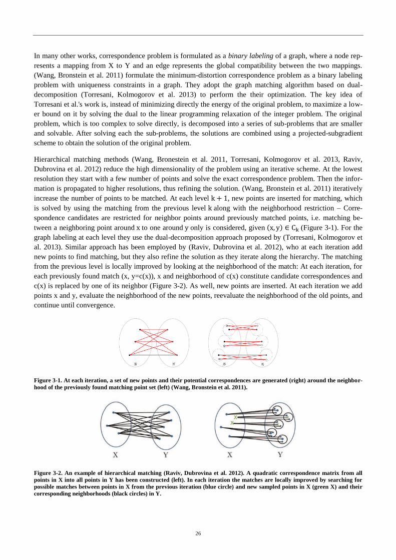
spondence candidates are restricted for neighbor points around previously matched points, i.e. matching be-

tween a neighboring point around to one around only is considered, given (Figure 3-1). For the

graph labeling at each level they use the dual-decomposition approach proposed by (Torresani, Kolmogorov et

al. 2013). Similar approach has been employed by (Raviv, Dubrovina et al. 2012), who at each iteration add

new points to find matching, but they also refine the solution as they iterate along the hierarchy. The matching

from the previous level is locally improved by looking at the neighborhood of the match: At each iteration, for

each previously found match (x, y=c(x)), x and neighborhood of c(x) constitute candidate correspondences and

c(x) is replaced by one of its neighbor (Figure 3-2). As well, new points are inserted. At each iteration we add

points x and y, evaluate the neighborhood of the new points, reevaluate the neighborhood of the old points, and

continue until convergence.

Figure 3-1. At each iteration, a set of new points and their potential correspondences are generated (right) around the neighbor-

hood of the previously found matching point set (left) (Wang, Bronstein et al. 2011).

Figure 3-2. An example of hierarchical matching (Raviv, Dubrovina et al. 2012). A quadratic correspondence matrix from all

points in X into all points in Y has been constructed (left). In each iteration the matches are locally improved by searching for

possible matches between points in X from the previous iteration (blue circle) and new sampled points in X (green X) and their

corresponding neighborhoods (black circles) in Y.

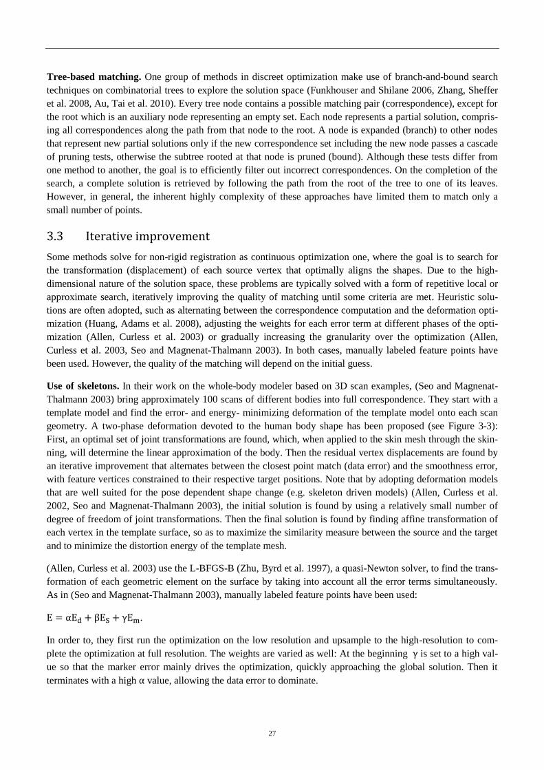
27

Tree-based matching. One group of methods in discreet optimization make use of branch-and-bound search

techniques on combinatorial trees to explore the solution space (Funkhouser and Shilane 2006, Zhang, Sheffer

et al. 2008, Au, Tai et al. 2010). Every tree node contains a possible matching pair (correspondence), except for

the root which is an auxiliary node representing an empty set. Each node represents a partial solution, compris-

ing all correspondences along the path from that node to the root. A node is expanded (branch) to other nodes

that represent new partial solutions only if the new correspondence set including the new node passes a cascade

of pruning tests, otherwise the subtree rooted at that node is pruned (bound). Although these tests differ from

one method to another, the goal is to efficiently filter out incorrect correspondences. On the completion of the

search, a complete solution is retrieved by following the path from the root of the tree to one of its leaves.

However, in general, the inherent highly complexity of these approaches have limited them to match only a

small number of points.

3.3 Iterative improvement

Some methods solve for non-rigid registration as continuous optimization one, where the goal is to search for

the transformation (displacement) of each source vertex that optimally aligns the shapes. Due to the high-

dimensional nature of the solution space, these problems are typically solved with a form of repetitive local or

approximate search, iteratively improving the quality of matching until some criteria are met. Heuristic solu-

tions are often adopted, such as alternating between the correspondence computation and the deformation opti-

mization (Huang, Adams et al. 2008), adjusting the weights for each error term at different phases of the opti-

mization (Allen, Curless et al. 2003) or gradually increasing the granularity over the optimization (Allen,

Curless et al. 2003, Seo and Magnenat-Thalmann 2003). In both cases, manually labeled feature points have

been used. However, the quality of the matching will depend on the initial guess.

Use of skeletons. In their work on the whole-body modeler based on 3D scan examples, (Seo and Magnenat-

Thalmann 2003) bring approximately 100 scans of different bodies into full correspondence. They start with a

template model and find the error- and energy- minimizing deformation of the template model onto each scan

geometry. A two-phase deformation devoted to the human body shape has been proposed (see Figure 3-3):

First, an optimal set of joint transformations are found, which, when applied to the skin mesh through the skin-

ning, will determine the linear approximation of the body. Then the residual vertex displacements are found by

an iterative improvement that alternates between the closest point match (data error) and the smoothness error,

with feature vertices constrained to their respective target positions. Note that by adopting deformation models

that are well suited for the pose dependent shape change (e.g. skeleton driven models) (Allen, Curless et al.

2002, Seo and Magnenat-Thalmann 2003), the initial solution is found by using a relatively small number of

degree of freedom of joint transformations. Then the final solution is found by finding affine transformation of

each vertex in the template surface, so as to maximize the similarity measure between the source and the target

and to minimize the distortion energy of the template mesh.

(Allen, Curless et al. 2003) use the L-BFGS-B (Zhu, Byrd et al. 1997), a quasi-Newton solver, to find the trans-

formation of each geometric element on the surface by taking into account all the error terms simultaneously.

As in (Seo and Magnenat-Thalmann 2003), manually labeled feature points have been used:

.

In order to, they first run the optimization on the low resolution and upsample to the high-resolution to com-

plete the optimization at full resolution. The weights are varied as well: At the beginning is set to a high val-

ue so that the marker error mainly drives the optimization, quickly approaching the global solution. Then it

terminates with a high value, allowing the data error to dominate.

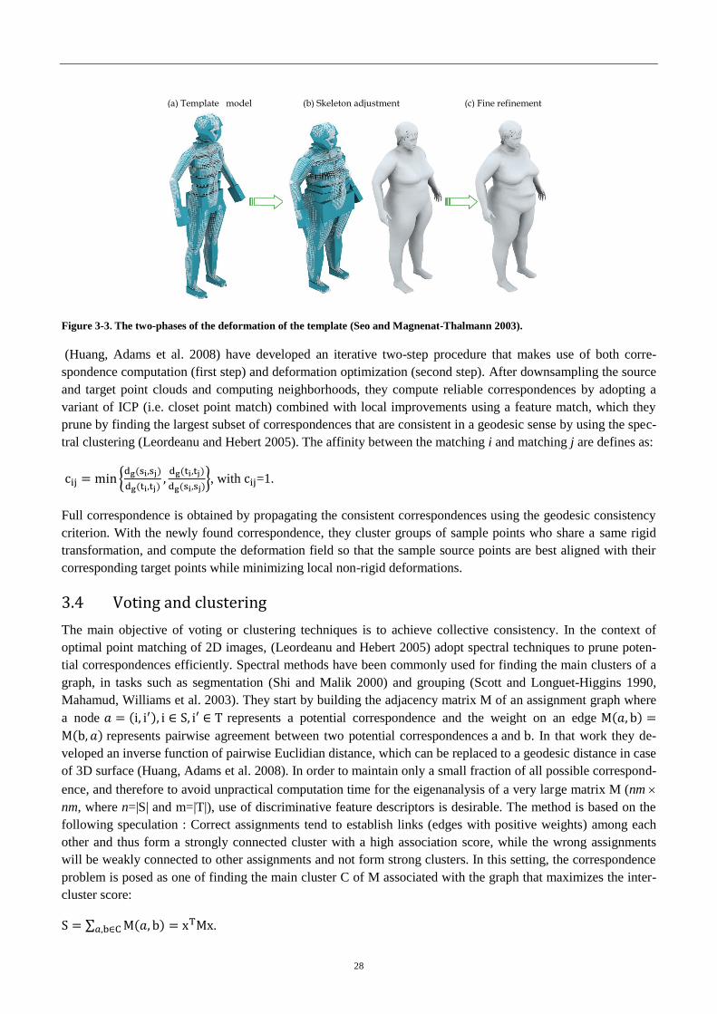
28

Figure 3-3. The two-phases of the deformation of the template (Seo and Magnenat-Thalmann 2003).

(Huang, Adams et al. 2008) have developed an iterative two-step procedure that makes use of both corre-

spondence computation (first step) and deformation optimization (second step). After downsampling the source

and target point clouds and computing neighborhoods, they compute reliable correspondences by adopting a

variant of ICP (i.e. closet point match) combined with local improvements using a feature match, which they

prune by finding the largest subset of correspondences that are consistent in a geodesic sense by using the spec-

tral clustering (Leordeanu and Hebert 2005). The affinity between the matching i and matching j are defines as:

, with =1.

Full correspondence is obtained by propagating the consistent correspondences using the geodesic consistency

criterion. With the newly found correspondence, they cluster groups of sample points who share a same rigid

transformation, and compute the deformation field so that the sample source points are best aligned with their

corresponding target points while minimizing local non-rigid deformations.

3.4 Voting and clustering

The main objective of voting or clustering techniques is to achieve collective consistency. In the context of

optimal point matching of 2D images, (Leordeanu and Hebert 2005) adopt spectral techniques to prune poten-

tial correspondences efficiently. Spectral methods have been commonly used for finding the main clusters of a

graph, in tasks such as segmentation (Shi and Malik 2000) and grouping (Scott and Longuet-Higgins 1990,

Mahamud, Williams et al. 2003). They start by building the adjacency matrix M of an assignment graph where

a node represents a potential correspondence and the weight on an edge

represents pairwise agreement between two potential correspondences and . In that work they de-

veloped an inverse function of pairwise Euclidian distance, which can be replaced to a geodesic distance in case

of 3D surface (Huang, Adams et al. 2008). In order to maintain only a small fraction of all possible correspond-

ence, and therefore to avoid unpractical computation time for the eigenanalysis of a very large matrix M (nm

nm, where n=|S| and m=|T|), use of discriminative feature descriptors is desirable. The method is based on the

following speculation : Correct assignments tend to establish links (edges with positive weights) among each

other and thus form a strongly connected cluster with a high association score, while the wrong assignments

will be weakly connected to other assignments and not form strong clusters. In this setting, the correspondence

problem is posed as one of finding the main cluster C of M associated with the graph that maximizes the inter-

cluster score:

.

(a) Template model (b) Skeleton adjustment (c) Fine refinement

29

The optimal solution x* is the binary vector that maximizes the score:

.

By relaxing the constraints on x, such that its elements can take real values in [0,1], they can find the solution

analytically, which is the principal eigenvector of M (by the Raleigh's ratio theorem). The eigenvector value

corresponding to a particular assignment a is interpreted as the confidence that a is a correct assignment. They

develop an iterative algorithm that binarizes the eigenvector by accepting assignments in an order of confi-

dence.

(Chang and Zwicker 2008) concentrate on the problem of finding the correspondence between two poses of an

articulated object, which they cast as that of choosing a set of optimal transformations among a set of predeter-

mined transformations that describe the partwise motion between the two poses. For each subsampled point in

the source shape, they find a set of potentially corresponding points in the target by computing the similarity

score based on the spin image (Johnson 1997). Then for each correspondence candidate (p,u), a rigid transfor-

mation from p to u is computed by combining the precomputed, per-vertex coordinate frames. They cluster the

computed set of transformations by using the mean-shift (Tuzel, Subbarao et al. 2005), from which they obtain

a pruned set of transformations (see Figure 3-4). Finally, the problem resorts to labeling each point in the

source with one of the selected transformations such that the feature similarity as well as smoothness is maxim-

ized, which they solve by using the graph cuts algorithm (Boykov, Veksler et al. 2001). However, such piece-

wise rigid motion assumption is not appropriate for deformable objects (i.e. human faces) or for different in-

stances of an object class (i.e. different horses) or even objects from different classes (horse and camel), related

by highly non-linear mappings.

Figure 3-4. (Chang and Zwicker 2008) cast the problem as that of choosing a set of optimal transformations via clustering.

Electors voting by (Au, Tai et al. 2010) finds sparse, semantic correspondence between the skeletons of two

models that are possibly geometrically very different. The electors (a large set of pruned correspondences) are

first selected via a combinatorial search with pruning tests designed to quickly prune out a majority of bad cor-

respondence. In order to maintain a reasonable size of the combinatorial solution space, they have used a skele-

ton structure composed of terminal (extremity) nodes and junction nodes (joints). On the completion of the

search, each node in the combinatorial tree represents an elector, which contains a series of correspondences

along the path from the root to that node. Each elector then casts one vote for each of its constituent matching

pair to establish the final correspondence. (Figure 3-5)

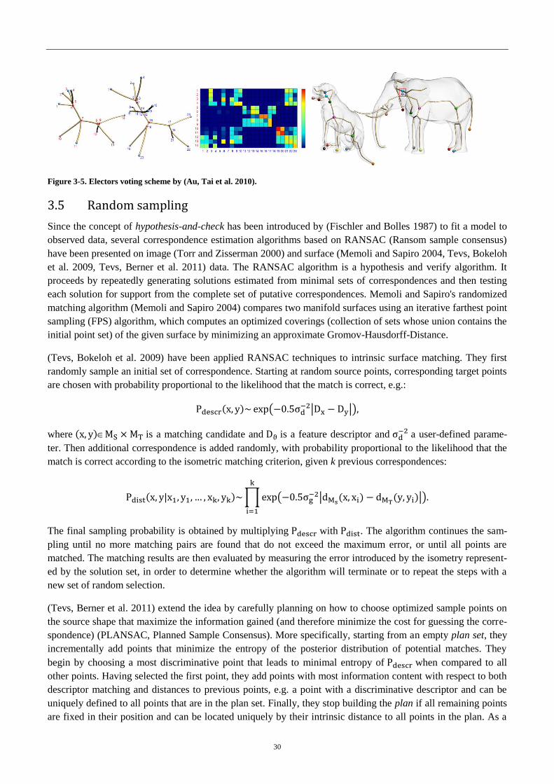
30

Figure 3-5. Electors voting scheme by (Au, Tai et al. 2010).

3.5 Random sampling

Since the concept of hypothesis-and-check has been introduced by (Fischler and Bolles 1987) to fit a model to

observed data, several correspondence estimation algorithms based on RANSAC (Ransom sample consensus)

have been presented on image (Torr and Zisserman 2000) and surface (Memoli and Sapiro 2004, Tevs, Bokeloh

et al. 2009, Tevs, Berner et al. 2011) data. The RANSAC algorithm is a hypothesis and verify algorithm. It

proceeds by repeatedly generating solutions estimated from minimal sets of correspondences and then testing

each solution for support from the complete set of putative correspondences. Memoli and Sapiro's randomized

matching algorithm (Memoli and Sapiro 2004) compares two manifold surfaces using an iterative farthest point

sampling (FPS) algorithm, which computes an optimized coverings (collection of sets whose union contains the

initial point set) of the given surface by minimizing an approximate Gromov-Hausdorff-Distance.

(Tevs, Bokeloh et al. 2009) have been applied RANSAC techniques to intrinsic surface matching. They first

randomly sample an initial set of correspondence. Starting at random source points, corresponding target points

are chosen with probability proportional to the likelihood that the match is correct, e.g.:

where is a matching candidate and is a feature descriptor and a user-defined parame-

ter. Then additional correspondence is added randomly, with probability proportional to the likelihood that the

match is correct according to the isometric matching criterion, given k previous correspondences:

The final sampling probability is obtained by multiplying with . The algorithm continues the sam-

pling until no more matching pairs are found that do not exceed the maximum error, or until all points are

matched. The matching results are then evaluated by measuring the error introduced by the isometry represent-

ed by the solution set, in order to determine whether the algorithm will terminate or to repeat the steps with a

new set of random selection.

(Tevs, Berner et al. 2011) extend the idea by carefully planning on how to choose optimized sample points on

the source shape that maximize the information gained (and therefore minimize the cost for guessing the corre-

spondence) (PLANSAC, Planned Sample Consensus). More specifically, starting from an empty plan set, they

incrementally add points that minimize the entropy of the posterior distribution of potential matches. They

begin by choosing a most discriminative point that leads to minimal entropy of when compared to all

other points. Having selected the first point, they add points with most information content with respect to both

descriptor matching and distances to previous points, e.g. a point with a discriminative descriptor and can be

uniquely defined to all points that are in the plan set. Finally, they stop building the plan if all remaining points

are fixed in their position and can be located uniquely by their intrinsic distance to all points in the plan. As a

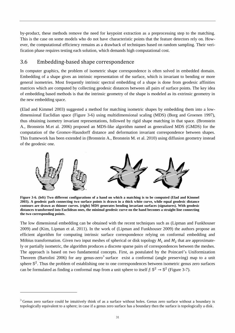
31

by-product, these methods remove the need for keypoint extraction as a preprocessing step to the matching.

This is the case on some models who do not have characteristic points that the feature detectors rely on. How-

ever, the computational efficiency remains as a drawback of techniques based on random sampling. Their veri-

fication phase requires testing each solution, which demands high computational cost.

3.6 Embedding-based shape correspondence

In computer graphics, the problem of isometric shape correspondence is often solved in embedded domain.

Embedding of a shape gives an intrinsic representation of the surface, which is invariant to bending or more

general isometries. Most frequently intrinsic spectral embedding of a shape is done from geodesic affinities

matrices which are computed by collecting geodesic distances between all pairs of surface points. The key idea

of embedding based methods is that the intrinsic geometry of the shape is modeled as its extrinsic geometry in

the new embedding space.

(Elad and Kimmel 2003) suggested a method for matching isometric shapes by embedding them into a low-

dimensional Euclidian space (Figure 3-6) using multidimensional scaling (MDS) (Borg and Groenen 1997),

thus obtaining isometry invariant representations, followed by rigid shape matching in that space. (Bronstein

A., Bronstein M.et al. 2006) proposed an MDS-like algorithm named as generalized MDS (GMDS) for the

computation of the Gromov-Hausdorff distance and deformation invariant correspondence between shapes.

This framework has been extended in (Bronstein A., Bronstein M. et al. 2010) using diffusion geometry instead

of the geodesic one.

Figure 3-6. (left) Two different configurations of a hand on which a matching is to be computed (Elad and Kimmel

2003). A geodesic path connecting two surface points is drawn in a thick white curve, while equal geodesic distance

contours are drawn as thinner curves. (right) MDS generates bending invariant surfaces (signatures). With geodesic

distances transformed into Euclidean ones, the minimal geodesic curve on the hand becomes a straight line connecting

the two corresponding points.

The low dimensional embedding can be obtained with the recent techniques such as (Lipman and Funkhouser

2009) and (Kim, Lipman et al. 2011). In the work of (Lipman and Funkhouser 2009) the authors propose an

efficient algorithm for computing intrinsic surface correspondence relying on conformal embedding and

Möbius transformation. Given two input meshes of spherical or disk topology and that are approximate-

ly or partially isometric, the algorithm produces a discrete sparse pairs of correspondences between the meshes.

The approach is based on two fundamental concepts. First, as postulated by the Poincaré’s Uniformization

Theorem (Bartolini 2006) for any genus-zero3 surface exist a conformal (angle preserving) map to a unit

sphere . Thus the problem of establishing one to one correspondences between isometric genus zero surfaces

can be formulated as finding a conformal map from a unit sphere to itself f: (Figure 3-7).

3 Genus zero surface could be intuitively think of as a surface without holes. Genus zero surface without a boundary is

topologically equivalent to a sphere; in case if a genus zero surface has a boundary then the surface is topologically a disk.

32

Figure 3-7. Isometric matching with Uniformization of surfaces: correspondence of two genus zero surfaces can be regarded as

conformal transformation of a unit sphere to itself (Lipman and Funkhouser 2009).

On the other hand, the group of all one to one conformal transformations m: forms Möbius group

which is well studied in geometry (Carne 2006). Since the Möbius group has six degrees of freedom, it is

sufficient to establish three unique correspondences in order to define the Möbius transformation m (MT). The

main implication of these observations is that establishing the entire map between isometric surfaces can be

done with just three point correspondences. More precisely, the algorithm proceeds as follows. Iteratively select

three distinct point pairs on the source and target. Compute Möbius transformation based on those point corre-

spondences. Use the obtained MT to transform all other points on the meshes. Then (Lipman and Funkhouser

2009) measure the deformation error between mapped points as deviation from isometry. The deformation er-

rors are accumulated in correspondence matrix C. Finally, based on confidence scores (the voting scores that

indicate the quality of correspondence) from the matrix C, the matching solution is extracted (Figure 3-8). The

algorithm performs the isometric shape matching in polynomial time with respect to number of vertices.

Figure 3-8. The pipeline of the Möbius voting algorithm (Lipman and Funkhouser 2009). Deformation errors of Möbius trans-

formations for the different triplets of initial correspondences are accumulated into correspondence matrix.

The follow up method of (Kim, Lipman et al. 2011) mends matching distortion of the conformal embedding

algorithm (Lipman and Funkhouser 2009) and establish reliable correspondences between not necessary iso-

metric surfaces. The key idea is to use a weighted combination of low-dimensional conformal correspondence

maps of Möbius voting in order to produce a so-called blended map which minimizes the mapping distortion

originating from violations of isometry.

Given the source and target surfaces with number of samples and correspondingly, the authors

compute first a set of candidate conformal maps

. Then for

each point on the source its correspondence is computed as a blended map that minimizes distor-

tion across the entire surface

,

(3-1)

where are so-called blended weights.

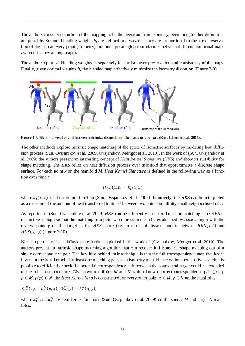
33

The authors consider distortion of the mapping to be the deviation from isometry, even though other definitions

are possible. Smooth blending weights are defined in a way that they are proportional to the area preserva-

tion of the map at every point (isometry), and incorporate global similarities between different conformal maps

(consistency among maps).

The authors optimize blending weights separately for the isometry preservation and consistency of the maps.

Finally, given optimal weights the blended map effectively minimize the isometry distortion (Figure 3-9).

Figure 3-9. Blending weights effectively minimize distortion of the maps (Kim, Lipman et al. 2011).

The other methods explore intrinsic shape matching of the space of isometric surfaces by modeling heat diffu-

sion process (Sun, Ovsjanikov et al. 2009, Ovsjanikov, Mérigot et al. 2010). In the work of (Sun, Ovsjanikov et

al. 2009) the authors present an interesting concept of Heat Kernel Signature (HKS) and show its suitability for

shape matching. The HKS relies on heat diffusion process over manifold that approximates a discrete shape

surface. For each point x on the manifold M, Heat Kernel Signature is defined in the following way as a func-

tion over time t

where is a heat kernel function (Sun, Ovsjanikov et al. 2009). Intuitively, the HKS can be interpreted

as a measure of the amount of heat transferred in time t between two points in infinity small neighborhood of x.

As reported in (Sun, Ovsjanikov et al. 2009) HKS can be efficiently used for the shape matching. The HKS is

distinctive enough so that the matching of a point x on the source can be established by associating x with the

nearest point y on the target in the HKS space (i.e. in terms of distance metric between and

) (Figure 3-10).

Nice properties of heat diffusion are further exploited in the work of (Ovsjanikov, Mérigot et al. 2010). The

authors present an intrinsic shape matching algorithm that can recover full isometric shape mapping out of a

single correspondence pair. The key idea behind their technique is that the full correspondence map that keeps

invariant the heat kernel of at least one matching pair is an isometry map. Hence without exhaustive search it is

possible to efficiently check if a potential correspondence pair between the source and target could be extended

to the full correspondence. Given two manifolds M and N with a known correct correspondence pair (p, q),

, the Heat Kernel Map is constructed for every other point on the manifolds

,

where and

are heat kernel functions (Sun, Ovsjanikov et al. 2009) on the source M and target N mani-

folds.

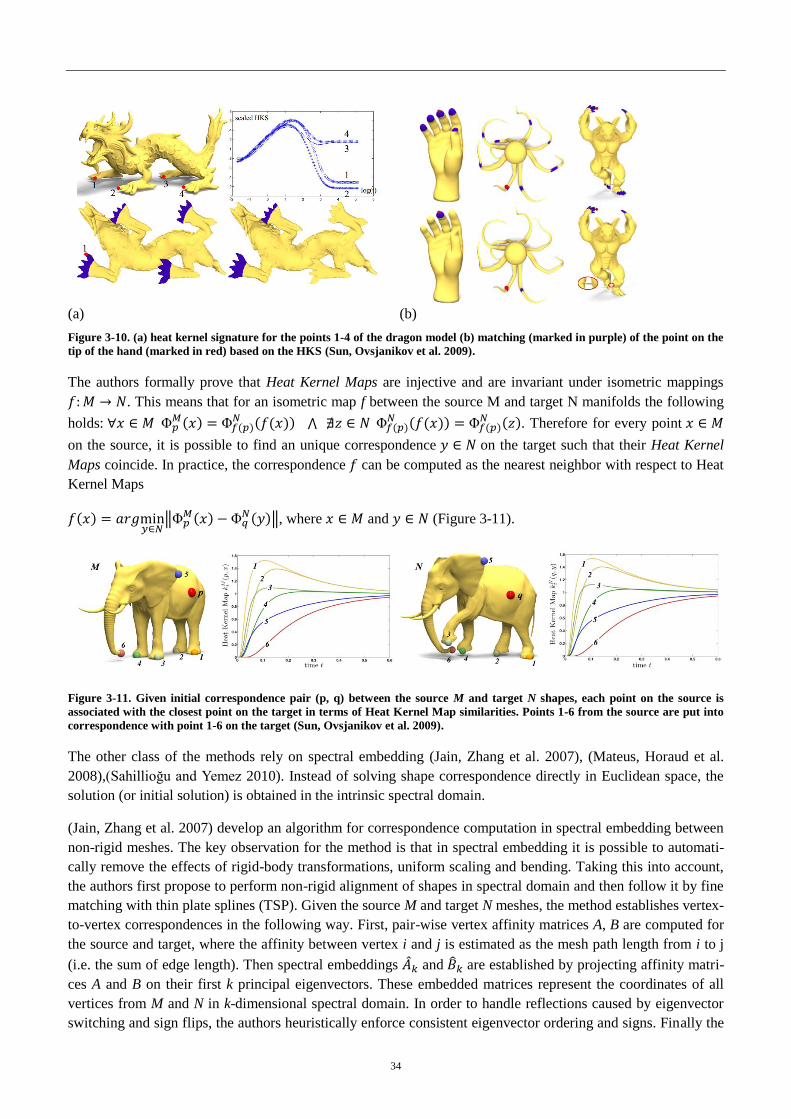
34

(a) (b)

Figure 3-10. (a) heat kernel signature for the points 1-4 of the dragon model (b) matching (marked in purple) of the point on the

tip of the hand (marked in red) based on the HKS (Sun, Ovsjanikov et al. 2009).

The authors formally prove that Heat Kernel Maps are injective and are invariant under isometric mappings

. This means that for an isometric map f between the source M and target N manifolds the following

holds:

. Therefore for every point

on the source, it is possible to find an unique correspondence on the target such that their Heat Kernel

Maps coincide. In practice, the correspondence can be computed as the nearest neighbor with respect to Heat

Kernel Maps

, where and (Figure 3-11).

Figure 3-11. Given initial correspondence pair (p, q) between the source M and target N shapes, each point on the source is

associated with the closest point on the target in terms of Heat Kernel Map similarities. Points 1-6 from the source are put into

correspondence with point 1-6 on the target (Sun, Ovsjanikov et al. 2009).

The other class of the methods rely on spectral embedding (Jain, Zhang et al. 2007), (Mateus, Horaud et al.

2008),(Sahillioğu and emez 2010). Instead of solving shape correspondence directly in Euclidean space, the

solution (or initial solution) is obtained in the intrinsic spectral domain.

(Jain, Zhang et al. 2007) develop an algorithm for correspondence computation in spectral embedding between

non-rigid meshes. The key observation for the method is that in spectral embedding it is possible to automati-

cally remove the effects of rigid-body transformations, uniform scaling and bending. Taking this into account,

the authors first propose to perform non-rigid alignment of shapes in spectral domain and then follow it by fine

matching with thin plate splines (TSP). Given the source M and target N meshes, the method establishes vertex-

to-vertex correspondences in the following way. First, pair-wise vertex affinity matrices A, B are computed for

the source and target, where the affinity between vertex i and j is estimated as the mesh path length from i to j

(i.e. the sum of edge length). Then spectral embeddings and are established by projecting affinity matri-

ces A and B on their first k principal eigenvectors. These embedded matrices represent the coordinates of all

vertices from M and N in k-dimensional spectral domain. In order to handle reflections caused by eigenvector

switching and sign flips, the authors heuristically enforce consistent eigenvector ordering and signs. Finally the

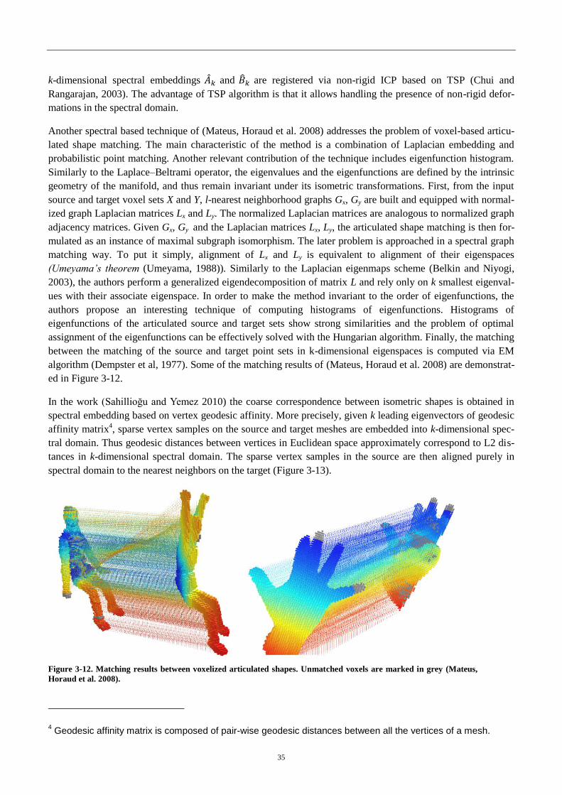
35

k-dimensional spectral embeddings and are registered via non-rigid ICP based on TSP (Chui and

Rangarajan, 2003). The advantage of TSP algorithm is that it allows handling the presence of non-rigid defor-

mations in the spectral domain.

Another spectral based technique of (Mateus, Horaud et al. 2008) addresses the problem of voxel-based articu-

lated shape matching. The main characteristic of the method is a combination of Laplacian embedding and

probabilistic point matching. Another relevant contribution of the technique includes eigenfunction histogram.

Similarly to the Laplace–Beltrami operator, the eigenvalues and the eigenfunctions are defined by the intrinsic

geometry of the manifold, and thus remain invariant under its isometric transformations. First, from the input

source and target voxel sets X and Y, l-nearest neighborhood graphs Gx, Gy are built and equipped with normal-

ized graph Laplacian matrices Lx and Ly. The normalized Laplacian matrices are analogous to normalized graph

adjacency matrices. Given Gx, Gy and the Laplacian matrices Lx, Ly, the articulated shape matching is then for-

mulated as an instance of maximal subgraph isomorphism. The later problem is approached in a spectral graph

matching way. To put it simply, alignment of Lx and Ly is equivalent to alignment of their eigenspaces

(Umeyama’s theorem (Umeyama, 1988)). Similarly to the Laplacian eigenmaps scheme (Belkin and Niyogi,

2003), the authors perform a generalized eigendecomposition of matrix L and rely only on k smallest eigenval-

ues with their associate eigenspace. In order to make the method invariant to the order of eigenfunctions, the

authors propose an interesting technique of computing histograms of eigenfunctions. Histograms of

eigenfunctions of the articulated source and target sets show strong similarities and the problem of optimal

assignment of the eigenfunctions can be effectively solved with the Hungarian algorithm. Finally, the matching

between the matching of the source and target point sets in k-dimensional eigenspaces is computed via EM

algorithm (Dempster et al, 1977). Some of the matching results of (Mateus, Horaud et al. 2008) are demonstrat-

ed in Figure 3-12.

In the work (Sahillioğu and emez 2010) the coarse correspondence between isometric shapes is obtained in

spectral embedding based on vertex geodesic affinity. More precisely, given k leading eigenvectors of geodesic

affinity matrix4, sparse vertex samples on the source and target meshes are embedded into k-dimensional spec-

tral domain. Thus geodesic distances between vertices in Euclidean space approximately correspond to L2 dis-

tances in k-dimensional spectral domain. The sparse vertex samples in the source are then aligned purely in

spectral domain to the nearest neighbors on the target (Figure 3-13).

Figure 3-12. Matching results between voxelized articulated shapes. Unmatched voxels are marked in grey (Mateus,

Horaud et al. 2008).

4 Geodesic affinity matrix is composed of pair-wise geodesic distances between all the vertices of a mesh.

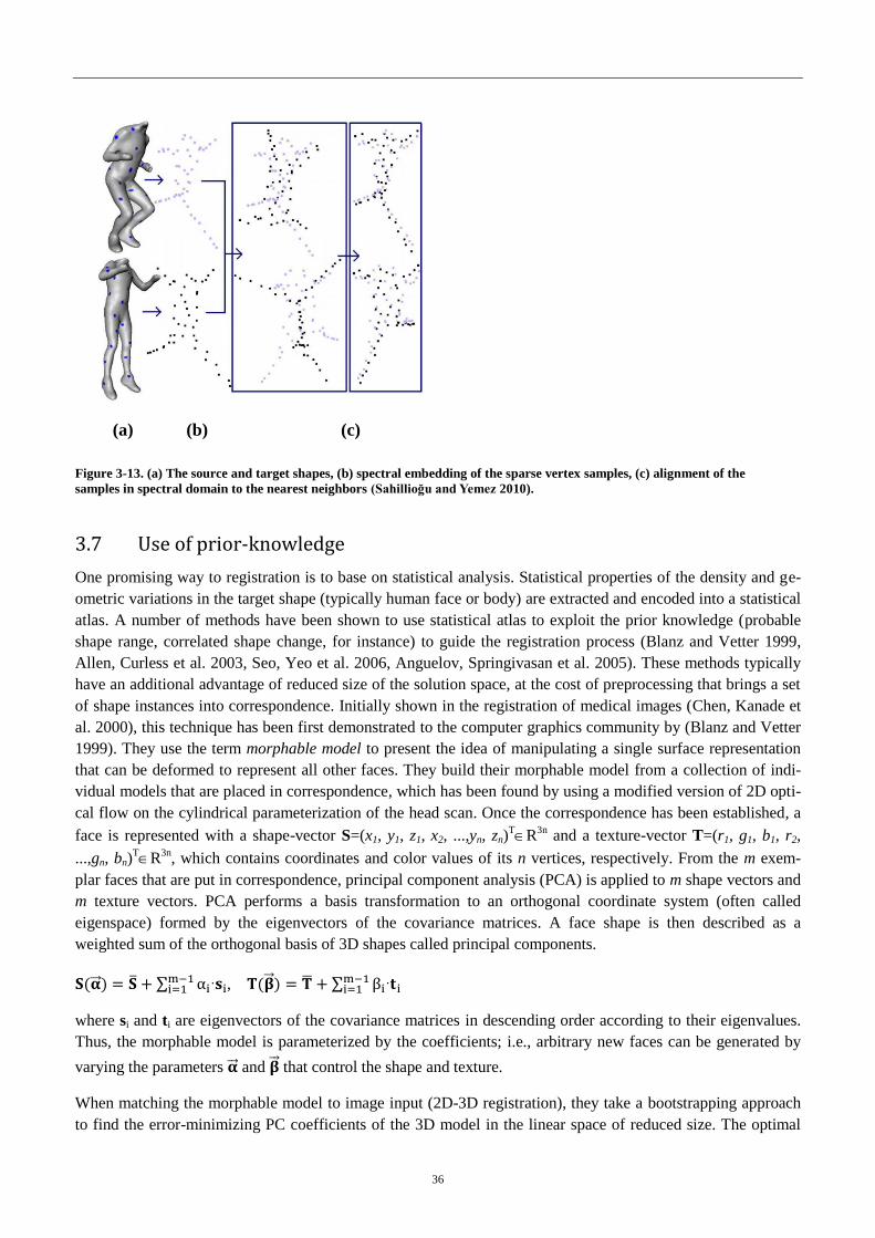
36

(a) (b) (c)

Figure 3-13. (a) The source and target shapes, (b) spectral embedding of the sparse vertex samples, (c) alignment of the

samples in spectral domain to the nearest neighbors 2010).

3.7 Use of prior-knowledge

One promising way to registration is to base on statistical analysis. Statistical properties of the density and ge-

ometric variations in the target shape (typically human face or body) are extracted and encoded into a statistical

atlas. A number of methods have been shown to use statistical atlas to exploit the prior knowledge (probable

shape range, correlated shape change, for instance) to guide the registration process (Blanz and Vetter 1999,

Allen, Curless et al. 2003, Seo, Yeo et al. 2006, Anguelov, Springivasan et al. 2005). These methods typically

have an additional advantage of reduced size of the solution space, at the cost of preprocessing that brings a set

of shape instances into correspondence. Initially shown in the registration of medical images (Chen, Kanade et

al. 2000), this technique has been first demonstrated to the computer graphics community by (Blanz and Vetter

1999). They use the term morphable model to present the idea of manipulating a single surface representation

that can be deformed to represent all other faces. They build their morphable model from a collection of indi-

vidual models that are placed in correspondence, which has been found by using a modified version of 2D opti-

cal flow on the cylindrical parameterization of the head scan. Once the correspondence has been established, a

face is represented with a shape-vector S=(x1, y1, z1, x2, ...,yn, zn)T R

3n and a texture-vector T=(r1, g1, b1, r2,

...,gn, bn)T R

3n, which contains coordinates and color values of its n vertices, respectively. From the m exem-

plar faces that are put in correspondence, principal component analysis (PCA) is applied to m shape vectors and

m texture vectors. PCA performs a basis transformation to an orthogonal coordinate system (often called

eigenspace) formed by the eigenvectors of the covariance matrices. A face shape is then described as a

weighted sum of the orthogonal basis of 3D shapes called principal components.

,

where si and ti are eigenvectors of the covariance matrices in descending order according to their eigenvalues.

Thus, the morphable model is parameterized by the coefficients; i.e., arbitrary new faces can be generated by

varying the parameters and that control the shape and texture.

When matching the morphable model to image input (2D-3D registration), they take a bootstrapping approach

to find the error-minimizing PC coefficients of the 3D model in the linear space of reduced size. The optimal

37

coefficients of the 3D model along with a set of rendering parameters are found such that they produce an im-

age as close as possible to the input image. In their analysis-by-synthesis loop, the algorithm creates a texture

mapped 3D face from the current model parameters, renders an image, and updates the parameters according to

the residual difference. It starts with the average head and with rendering parameters roughly estimated by the

user. Similarly, when matching the morphable model to a 3D scan (3D-3D registration), they search for optimal

coefficients that minimize the color error between the corresponding points.

Later, similar approach has been demonstrated by (Allen, Curless at al. 2003) (markerless matching) and (Seo,

Yeo et al. 2006) (image guided reconstruction of human body shapes). Given a set of example body shapes

represented as vectors, they apply PCA to them to obtain linear shape spaces. As has been the case with the

morphable face model, such shape space allows not only to systematically observe the diversity and individual-

ity of shapes, but also to generate a new, plausible individual shape in an easier and simpler manner. When

computing for the optimal set of coefficients, a new error term indicating the likelihood of a particular set of

PCA coefficients is introduced:

The SCAPE approach of (Anguelov, Springivasan et al. 2005) propose combined models that learn both static

(identity-dependent) and dynamic (movement-dependent) shape variation have been suggested, allowing to

generate shapes of any identity in any pose. SCAPE learns pose-deformation as completely separate phenome-

non from the PCA-based identify variation model, and then combines the two modalities when a new shape is

synthesized. Though very powerful, it cannot capture the correlation between the two modalities. For example,

when a muscular person bends his/her arm, the shape change will be the same as when a very thin person bends

the arm. Vlasic et al’s multilinear models (Vlasic, Brand et al. 2005) has shown how multilinear algebra could

be adopted to extend latent variable techniques to handle multiple modalities, such as identity, expression, and

viseme of a face. Later, (Allen, Curless et al. 2006) propose to capture both identity-dependent and pose-

dependent shape variation in a correlated fashion. By incorporating the two entities that have previously han-

dled separately into a single model, the model is potentially more expressive and realistic for synthesizing and

editing animated characters.

38

Chapter 4 Feature detection for animated

meshes

4.1 Introduction

In this chapter we present a novel technique of dynamic feature detection for animated meshes. Since such data

has considerably large sizes, it often becomes indispensable to be able to select distinctive features from it, so

as to maintain efficiency in its representation and in the process applied to it. Consequently, the need for robust,

repeatable, and consistent detection of meaningful features from animation data cannot be overemphasized.

However, the feature detection in animated mesh remains as much less explored domain, despite the prolifera-

tion of feature detectors developed by many researchers in computer graphics and computer vision. As we ex-

plained in Chapter 2, dynamic feature points have a potential to bring a particularly remarkable value to time-

varying animated animated mesh correspondence. Being able to extract repeatable coherent sets of dynamic

features and to establish reliable correspondences between them (as detailed in Chapter 5), facilitates signifi-

cantly dynamic shape matching.

Feature point extraction has been a long-studied subject in computer vision, image processing and computer

graphics. Traditionally, features are often extracted from different modalities and graphical entities such as

2d/3d images, videos, polygonal meshes and point clouds. Therefore it is especially unfortunate that a problem

of feature point detection on animated meshes remains unstudied. While classical feature points are directly

related to static local neighbourhood and geometry, we proposed a novel feature detection technique based on

dynamic behaviour of the shape and its deformation characteristics.

Chapter 4 details a new feature extraction method on animated meshes in the following way:

1. We survey related works on feature extraction for (static) meshes and videos, which are the most

closely related to our work (Section 4.2)

2. Describe the deformation characteristics and how they are captured (Section 4.4)

3. Outline the basics of linear scale-space theory (Section 4.5)

4. Establish a novel spatio-temporal Difference of Gaussians (DoG) operator (Section 4.7)

5. Show results of proposed feature point extraction algorithm and evaluate robustness of the method

(Sections 4.8, 4.9)

In scope of this dissertation, we first develop a spatio-temporal feature detection framework on animated

meshes (an ordered sequence of static mesh frames with fixed number of vertices and connectivity), based on

the scale space approaches. Our feature detection scheme is then used for the sparse and dense dynamic shape

correspondence (Chapter 5). The algorithm, which we call AniM-DoG, extends the spatial interest point (IP)

detectors on static meshes (Pauly, Keiser et al. 2003, Castellani, Cristani et al. 2008, Zaharescu, Boyer et al.

2009, Darom and Keller 2012) so as to detect spatio-temporal feature points on animated meshes. Based on

deformation characterestics computed at each vertex in each frame, we build the scale space by computing

various smoothed versions of the given animation data. At the heart of our algorithm is a new space-time

Difference of Gaussian (DoG) operator, which approximates the spatio-temporal, scale-normalized Laplacian.

39

By computing local extrema of the new operator in space-time and scale, we obtain repeatable sets of spatio-

temporal feature points over different deforming surfaces modelled as triangle mesh animations. We then vali-

date the proposed AniM-DoG algorithm for its robustness and consistency. To the best of our knowledge, our

work is the first that addresses the spatio-temporal feature detector in animated meshes.

Our goal in this chapter is to develop a feature detector on animated mesh based on space-time DoG, which has

been reported to be efficient approximation of robust Laplacian blob detector in space domain. Note that ani-

mated meshes that we are dealing with are assumed to have no clutters or holes, and maintain fixed topology

over time, without tearing or changing genus. The spatial samplings can vary from one mesh to another, but it

is desirable to have uniform sampling across one surface. The temporal sampling rate can also vary (~30Hz in

our experiments), depending on how the animation has been obtained. In any case, the temporal sampling is

considered uniform.

The features we want to extract are the corners/blob-like structures, which are located in regions that exhibit a

high variation of deformation spatially and temporally. We first define local deformation attributes on the ani-

mated mesh, from which we build a multi-scale representation of it. One of the main motivations to base our

method on local surface deformation can be explained by the fact that (1) local deformation on a surface can be

effectively measured by some well-defined principles, and that (2) the domain has intrinsic dimension of

2D+time (rather than 3D+time) with some reasonable assumption on the data, i.e. differentiable compact 2-

manifold with time-varying embedding.

Since feature extraction in animated meshes is a relatively unexplored area we had some freedom to define the

approach to the problem. The goal is to build a powerful dynamic feature extraction framework that satisfies a

set of highly desirable requirements:

1. Capture animation deforming characteristics (Section 4.4)

2. Multiscale i.e. representing deforming structures at different scales (Section 4.6)

3. Robust to noise and geometry variations (Section 4.9)

4. Consistent and repeatable over semantically similar mesh animations (Section 4.9.1)

5. Meaningful for human perception (Section 4.9.2)

We addressed those requirements within a scope of different applied mathematical fields: mechanics, differen-

tial geometry, linear scale space theory and signal processing. First, the items 1, 4, 5 require to analyze and

numerically measure the deformation of the animated mesh shape. Inter frame vertex displacement i.e. velocity

or acceleration can be used to quantify the motion (Bulbul, Koca et al. 2010). However it can over-emphasize

the saliency of rigidly moving animated mesh parts, which is undesirable. We propose to use local triangle

strains as a surface deformation characteristic. By definition triangle strain carries only pure non-rigid deforma-

tion measure. We further improve the deformation characteristics robustness by fusing triangle strain with the

mean curvature change. The later allows us to quantitively capture approximately isometric deformations such

as bending. Such deformation characteristics, as we show in evaluation of the method, also coherent with hu-

man eye perception of deforming mesh. Second, we would like the dynamic feature point to carry the informa-

tion about spatio and temporal extents of deformation exhibited in a place of feature detection. Further we

proved being correct to use math tools from linear scale space theory in order to address feature multiscale rep-

resentation (Section 4.6). Linear scale space theory is a subset of scale space frameworks developed in Com-

puter Vision community in 1980s. During the past decade it attracted attention in point-sampled and polygonal

surface analysis. In this thesis we define scale space mechanisms for feature point extraction from animated

meshes.

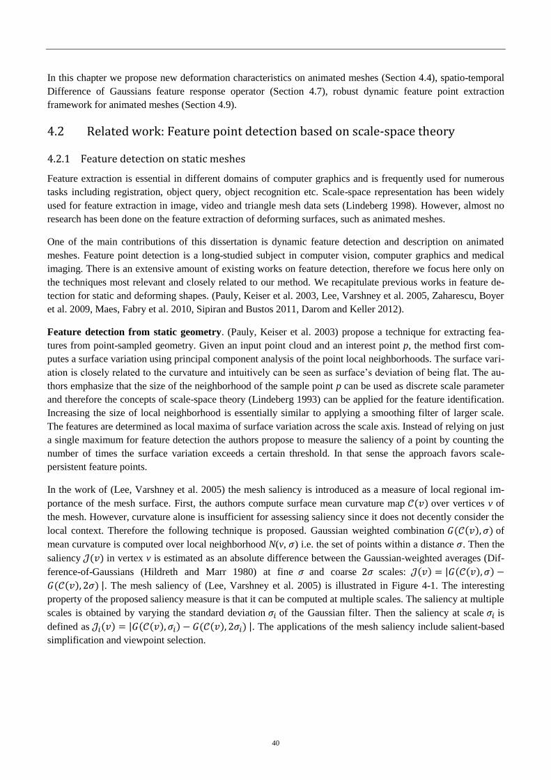
40

In this chapter we propose new deformation characteristics on animated meshes (Section 4.4), spatio-temporal

Difference of Gaussians feature response operator (Section 4.7), robust dynamic feature point extraction

framework for animated meshes (Section 4.9).

4.2 Related work: Feature point detection based on scale-space theory

4.2.1 Feature detection on static meshes

Feature extraction is essential in different domains of computer graphics and is frequently used for numerous

tasks including registration, object query, object recognition etc. Scale-space representation has been widely

used for feature extraction in image, video and triangle mesh data sets (Lindeberg 1998). However, almost no

research has been done on the feature extraction of deforming surfaces, such as animated meshes.

One of the main contributions of this dissertation is dynamic feature detection and description on animated

meshes. Feature point detection is a long-studied subject in computer vision, computer graphics and medical

imaging. There is an extensive amount of existing works on feature detection, therefore we focus here only on

the techniques most relevant and closely related to our method. We recapitulate previous works in feature de-

tection for static and deforming shapes. (Pauly, Keiser et al. 2003, Lee, Varshney et al. 2005, Zaharescu, Boyer

et al. 2009, Maes, Fabry et al. 2010, Sipiran and Bustos 2011, Darom and Keller 2012).

Feature detection from static geometry. (Pauly, Keiser et al. 2003) propose a technique for extracting fea-

tures from point-sampled geometry. Given an input point cloud and an interest point p, the method first com-

putes a surface variation using principal component analysis of the point local neighborhoods. The surface vari-

ation is closely related to the curvature and intuitively can be seen as surface’s deviation of being flat. The au-

thors emphasize that the size of the neighborhood of the sample point p can be used as discrete scale parameter

and therefore the concepts of scale-space theory (Lindeberg 1993) can be applied for the feature identification.

Increasing the size of local neighborhood is essentially similar to applying a smoothing filter of larger scale.

The features are determined as local maxima of surface variation across the scale axis. Instead of relying on just

a single maximum for feature detection the authors propose to measure the saliency of a point by counting the

number of times the surface variation exceeds a certain threshold. In that sense the approach favors scale-

persistent feature points.

In the work of (Lee, Varshney et al. 2005) the mesh saliency is introduced as a measure of local regional im-

portance of the mesh surface. First, the authors compute surface mean curvature map over vertices v of

the mesh. However, curvature alone is insufficient for assessing saliency since it does not decently consider the

local context. Therefore the following technique is proposed. Gaussian weighted combination of

mean curvature is computed over local neighborhood N(v, ) i.e. the set of points within a distance . Then the

saliency in vertex v is estimated as an absolute difference between the Gaussian-weighted averages (Dif-

ference-of-Gaussians (Hildreth and Marr 1980) at fine and coarse scales:

. The mesh saliency of (Lee, Varshney et al. 2005) is illustrated in Figure 4-1. The interesting

property of the proposed saliency measure is that it can be computed at multiple scales. The saliency at multiple

scales is obtained by varying the standard deviation of the Gaussian filter. Then the saliency at scale is

defined as . The applications of the mesh saliency include salient-based

simplification and viewpoint selection.

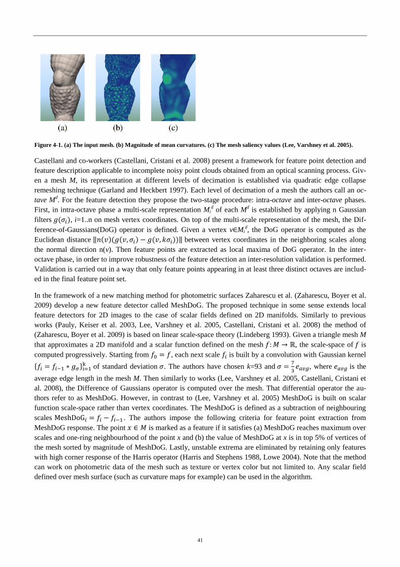
41

Figure 4-1. (a) The input mesh. (b) Magnitude of mean curvatures. (c) The mesh saliency values (Lee, Varshney et al. 2005).

Castellani and co-workers (Castellani, Cristani et al. 2008) present a framework for feature point detection and

feature description applicable to incomplete noisy point clouds obtained from an optical scanning process. Giv-

en a mesh M, its representation at different levels of decimation is established via quadratic edge collapse

remeshing technique (Garland and Heckbert 1997). Each level of decimation of a mesh the authors call an oc-

tave Md. For the feature detection they propose the two-stage procedure: intra-octave and inter-octave phases.

First, in intra-octave phase a multi-scale representation Mid of each M

d is established by applying n Gaussian

filters , i=1..n on mesh vertex coordinates. On top of the multi-scale representation of the mesh, the Dif-

ference-of-Gaussians(DoG) operator is defined. Given a vertex v Mid, the DoG operator is computed as the

Euclidean distance between vertex coordinates in the neighboring scales along

the normal direction n(v). Then feature points are extracted as local maxima of DoG operator. In the inter-

octave phase, in order to improve robustness of the feature detection an inter-resolution validation is performed.

Validation is carried out in a way that only feature points appearing in at least three distinct octaves are includ-

ed in the final feature point set.

In the framework of a new matching method for photometric surfaces Zaharescu et al. (Zaharescu, Boyer et al.

2009) develop a new feature detector called MeshDoG. The proposed technique in some sense extends local

feature detectors for 2D images to the case of scalar fields defined on 2D manifolds. Similarly to previous

works (Pauly, Keiser et al. 2003, Lee, Varshney et al. 2005, Castellani, Cristani et al. 2008) the method of

(Zaharescu, Boyer et al. 2009) is based on linear scale-space theory (Lindeberg 1993). Given a triangle mesh M

that approximates a 2D manifold and a scalar function defined on the mesh , the scale-space of is

computed progressively. Starting from , each next scale is built by a convolution with Gaussian kernel

of standard deviation . The authors have chosen k=93 and

, where is the

average edge length in the mesh M. Then similarly to works (Lee, Varshney et al. 2005, Castellani, Cristani et

al. 2008), the Difference of Gaussians operator is computed over the mesh. That differential operator the au-

thors refer to as MeshDoG. However, in contrast to (Lee, Varshney et al. 2005) MeshDoG is built on scalar

function scale-space rather than vertex coordinates. The MeshDoG is defined as a subtraction of neighbouring

scales . The authors impose the following criteria for feature point extraction from

MeshDoG response. The point is marked as a feature if it satisfies (a) MeshDoG reaches maximum over

scales and one-ring neighbourhood of the point x and (b) the value of MeshDoG at x is in top 5% of vertices of

the mesh sorted by magnitude of MeshDoG. Lastly, unstable extrema are eliminated by retaining only features

with high corner response of the Harris operator (Harris and Stephens 1988, Lowe 2004). Note that the method

can work on photometric data of the mesh such as texture or vertex color but not limited to. Any scalar field

defined over mesh surface (such as curvature maps for example) can be used in the algorithm.

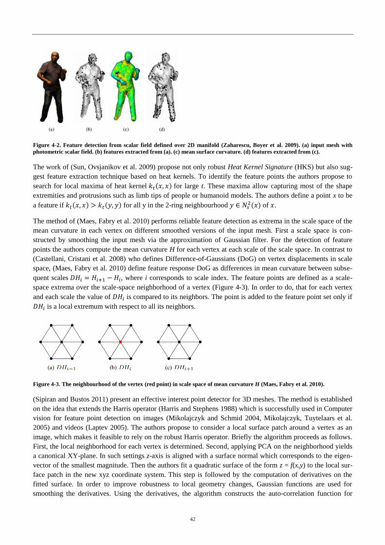
42

Figure 4-2. Feature detection from scalar field defined over 2D manifold (Zaharescu, Boyer et al. 2009). (a) input mesh with

photometric scalar field. (b) features extracted from (a). (c) mean surface curvature. (d) features extracted from (c).

The work of (Sun, Ovsjanikov et al. 2009) propose not only robust Heat Kernel Signature (HKS) but also sug-

gest feature extraction technique based on heat kernels. To identify the feature points the authors propose to

search for local maxima of heat kernel for large t. These maxima allow capturing most of the shape

extremities and protrusions such as limb tips of people or humanoid models. The authors define a point x to be

a feature if for all y in the 2-ring neighbourhood of .

The method of (Maes, Fabry et al. 2010) performs reliable feature detection as extrema in the scale space of the

mean curvature in each vertex on different smoothed versions of the input mesh. First a scale space is con-

structed by smoothing the input mesh via the approximation of Gaussian filter. For the detection of feature

points the authors compute the mean curvature H for each vertex at each scale of the scale space. In contrast to

(Castellani, Cristani et al. 2008) who defines Difference-of-Gaussians (DoG) on vertex displacements in scale

space, (Maes, Fabry et al. 2010) define feature response DoG as differences in mean curvature between subse-

quent scales , where i corresponds to scale index. The feature points are defined as a scale-

space extrema over the scale-space neighborhood of a vertex (Figure 4-3). In order to do, that for each vertex

and each scale the value of is compared to its neighbors. The point is added to the feature point set only if

is a local extremum with respect to all its neighbors.

Figure 4-3. The neighbourhood of the vertex (red point) in scale space of mean curvature H (Maes, Fabry et al. 2010).

(Sipiran and Bustos 2011) present an effective interest point detector for 3D meshes. The method is established

on the idea that extends the Harris operator (Harris and Stephens 1988) which is successfully used in Computer

vision for feature point detection on images (Mikolajczyk and Schmid 2004, Mikolajczyk, Tuytelaars et al.

2005) and videos (Laptev 2005). The authors propose to consider a local surface patch around a vertex as an

image, which makes it feasible to rely on the robust Harris operator. Briefly the algorithm proceeds as follows.

First, the local neighborhood for each vertex is determined. Second, applying PCA on the neighborhood yields

a canonical XY-plane. In such settings z-axis is aligned with a surface normal which corresponds to the eigen-

vector of the smallest magnitude. Then the authors fit a quadratic surface of the form z = f(x,y) to the local sur-

face patch in the new xyz coordinate system. This step is followed by the computation of derivatives on the

fitted surface. In order to improve robustness to local geometry changes, Gaussian functions are used for

smoothing the derivatives. Using the derivatives, the algorithm constructs the auto-correlation function for

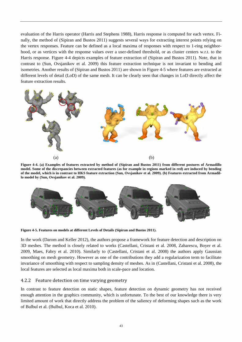
43

evaluation of the Harris operator (Harris and Stephens 1988), Harris response is computed for each vertex. Fi-

nally, the method of (Sipiran and Bustos 2011) suggests several ways for extracting interest points relying on

the vertex responses. Feature can be defined as a local maxima of responses with respect to 1-ring neighbor-

hood, or as vertices with the response values over a user-defined threshold, or as cluster centers w.r.t. to the

Harris response. Figure 4-4 depicts examples of feature extraction of (Sipiran and Bustos 2011). Note, that in

contrast to (Sun, Ovsjanikov et al. 2009) this feature extraction technique is not invariant to bending and

isometries. Another results of (Sipiran and Bustos 2011) are shown in Figure 4-5 where features are extracted at

different levels of detail (LoD) of the same mesh. It can be clearly seen that changes in LoD directly affect the

feature extraction results.

(a) (b)

Figure 4-4. (a) Examples of features extracted by method of (Sipiran and Bustos 2011) from different postures of Armadillo

model. Some of the discrepancies between extracted features (as for example in regions marked in red) are induced by bending

of the model, which is in contrast to HKS feature extraction (Sun, Ovsjanikov et al. 2009). (b) Features extracted from Armadil-

lo model by (Sun, Ovsjanikov et al. 2009).

Figure 4-5. Features on models at different Levels of Details (Sipiran and Bustos 2011).

In the work (Darom and Keller 2012), the authors propose a framework for feature detection and description on

3D meshes. The method is closely related to works (Castellani, Cristani et al. 2008, Zaharescu, Boyer et al.

2009, Maes, Fabry et al. 2010). Similarly to (Castellani, Cristani et al. 2008) the authors apply Gaussian

smoothing on mesh geometry. However as one of the contributions they add a regularization term to facilitate

invariance of smoothing with respect to sampling density of meshes. As in (Castellani, Cristani et al. 2008), the

local features are selected as local maxima both in scale-pace and location.

4.2.2 Feature detection on time varying geometry

In contrast to feature detection on static shapes, feature detection on dynamic geometry has not received

enough attention in the graphics community, which is unfortunate. To the best of our knowledge there is very

limited amount of work that directly address the problem of the saliency of deforming shapes such as the work

of Bulbul et al. (Bulbul, Koca et al. 2010).

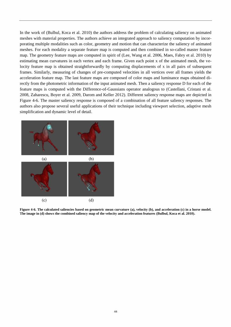
44

In the work of (Bulbul, Koca et al. 2010) the authors address the problem of calculating saliency on animated

meshes with material properties. The authors achieve an integrated approach to saliency computation by incor-

porating multiple modalities such as color, geometry and motion that can characterize the saliency of animated

meshes. For each modality a separate feature map is computed and then combined in so-called master feature

map. The geometry feature maps are computed in spirit of (Lee, Wang et al. 2006, Maes, Fabry et al. 2010) by

estimating mean curvatures in each vertex and each frame. Given each point x of the animated mesh, the ve-

locity feature map is obtained straightforwardly by computing displacements of x in all pairs of subsequent

frames. Similarly, measuring of changes of pre-computed velocities in all vertices over all frames yields the

acceleration feature map. The last feature maps are composed of color maps and luminance maps obtained di-

rectly from the photometric information of the input animated mesh. Then a saliency response D for each of the

feature maps is computed with the Difference-of-Gaussians operator analogous to (Castellani, Cristani et al.

2008, Zaharescu, Boyer et al. 2009, Darom and Keller 2012). Different saliency response maps are depicted in

Figure 4-6. The master saliency response is composed of a combination of all feature saliency responses. The

authors also propose several useful applications of their technique including viewport selection, adaptive mesh

simplification and dynamic level of detail.

Figure 4-6. The calculated saliencies based on geometric mean curvature (a), velocity (b), and acceleration (c) in a horse model.

The image in (d) shows the combined saliency map of the velocity and acceleration features (Bulbul, Koca et al. 2010).

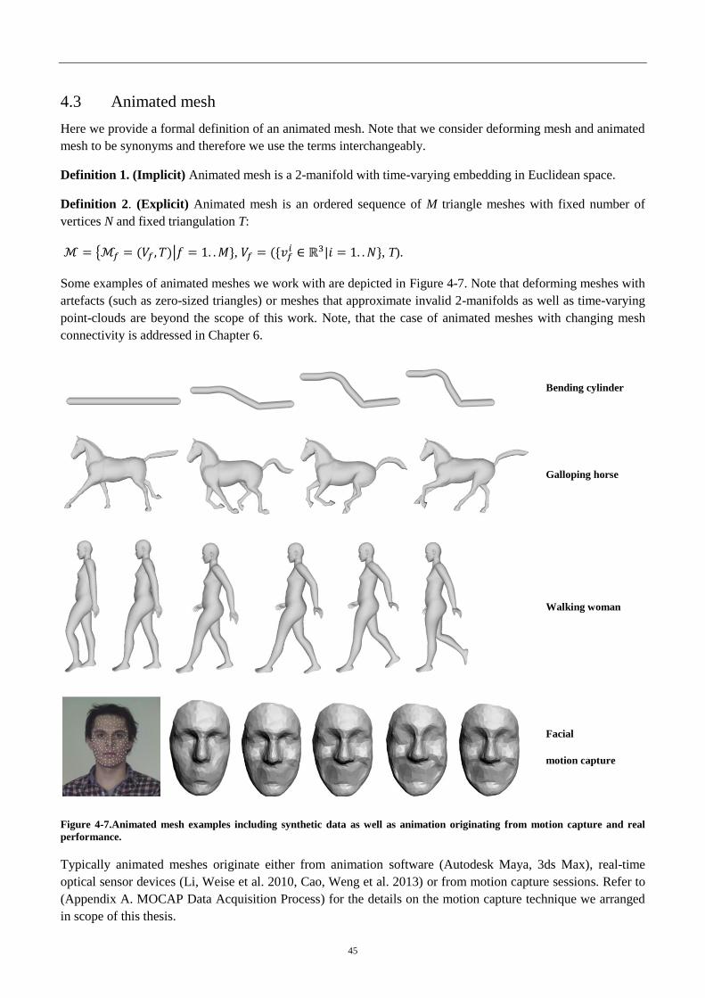
45

4.3 Animated mesh

Here we provide a formal definition of an animated mesh. Note that we consider deforming mesh and animated

mesh to be synonyms and therefore we use the terms interchangeably.

Definition 1. (Implicit) Animated mesh is a 2-manifold with time-varying embedding in Euclidean space.

Definition 2. (Explicit) Animated mesh is an ordered sequence of M triangle meshes with fixed number of

vertices N and fixed triangulation T:

, , T).

Some examples of animated meshes we work with are depicted in Figure 4-7. Note that deforming meshes with

artefacts (such as zero-sized triangles) or meshes that approximate invalid 2-manifolds as well as time-varying

point-clouds are beyond the scope of this work. Note, that the case of animated meshes with changing mesh

connectivity is addressed in Chapter 6.

Bending cylinder

Galloping horse

Walking woman

Facial

motion capture

Figure 4-7.Animated mesh examples including synthetic data as well as animation originating from motion capture and real

performance.

Typically animated meshes originate either from animation software (Autodesk Maya, 3ds Max), real-time

optical sensor devices (Li, Weise et al. 2010, Cao, Weng et al. 2013) or from motion capture sessions. Refer to

(Appendix A. MOCAP Data Acquisition Process) for the details on the motion capture technique we arranged

in scope of this thesis.

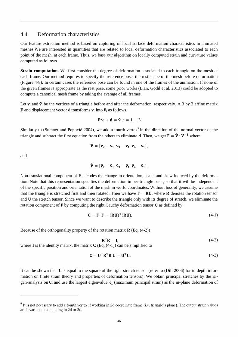
46

4.4 Deformation characteristics

Our feature extraction method is based on capturing of local surface deformation characteristics in animated

meshes.We are interested in quantities that are related to local deformation characteristics associated to each

point of the mesh, at each frame. Thus, we base our algorithm on locally computed strain and curvature values

computed as follows.

Strain computation. We first consider the degree of deformation associated to each triangle on the mesh at

each frame. Our method requires to specify the reference pose, the rest shape of the mesh before deformation

(Figure 4-8). In certain cases the reference pose can be found in one of the frames of the animation. If none of

the given frames is appropriate as the rest pose, some prior works (Lian, Godil et al. 2013) could be adopted to

compute a canonical mesh frame by taking the average of all frames.

Let and be the vertices of a triangle before and after the deformation, respectively. A 3 by 3 affine matrix

F and displacement vector d transforms into as follows.

Similarly to (Sumner and Popović 2004), we add a fourth vertex5 in the direction of the normal vector of the

triangle and subtract the first equation from the others to eliminate d. Then, we get where

,

and

.

Non-translational component of F encodes the change in orientation, scale, and skew induced by the deforma-

tion. Note that this representation specifies the deformation in per-triangle basis, so that it will be independent

of the specific position and orientation of the mesh in world coordinates. Without loss of generality, we assume

that the triangle is stretched first and then rotated. Then we have , where R denotes the rotation tensor

and U the stretch tensor. Since we want to describe the triangle only with its degree of stretch, we eliminate the

rotation component of by computing the right Cauchy deformation tensor C as defined by:

. (4-1)

Because of the orthogonality property of the rotation matrix R (Eq. (4-2))

, (4-2)

where I is the identity matrix, the matrix C (Eq. (4-1)) can be simplified to

. (4-3)

It can be shown that is equal to the square of the right stretch tensor (refer to (Dill 2006) for in depth infor-

mation on finite strain theory and properties of deformation tensors). We obtain principal stretches by the Ei-

gen-analysis on , and use the largest eigenvalue (maximum principal strain) as the in-plane deformation of

5 It is not necessary to add a fourth vertex if working in 2d coordinate frame (i.e. triangle’s plane). The output strain values

are invariant to computing in 2d or 3d.

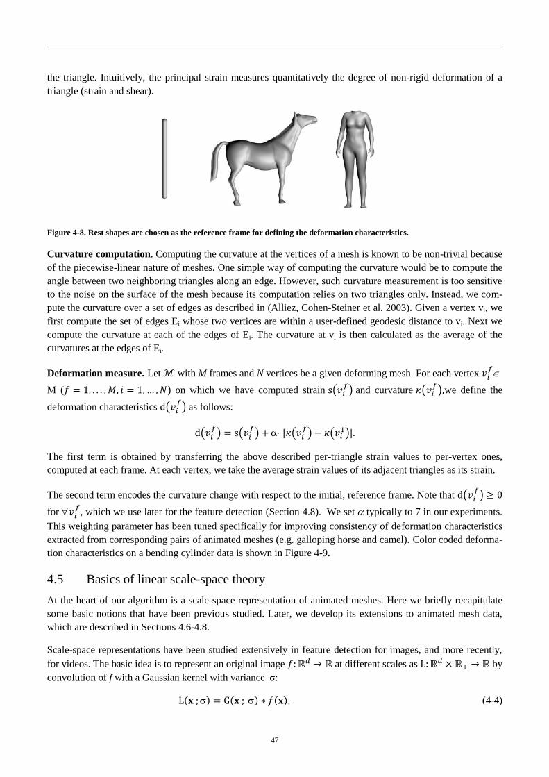
47

the triangle. Intuitively, the principal strain measures quantitatively the degree of non-rigid deformation of a

triangle (strain and shear).

Figure 4-8. Rest shapes are chosen as the reference frame for defining the deformation characteristics.

Curvature computation. Computing the curvature at the vertices of a mesh is known to be non-trivial because

of the piecewise-linear nature of meshes. One simple way of computing the curvature would be to compute the

angle between two neighboring triangles along an edge. However, such curvature measurement is too sensitive

to the noise on the surface of the mesh because its computation relies on two triangles only. Instead, we com-

pute the curvature over a set of edges as described in (Alliez, Cohen-Steiner et al. 2003). Given a vertex vi, we

first compute the set of edges Ei whose two vertices are within a user-defined geodesic distance to vi. Next we

compute the curvature at each of the edges of Ei. The curvature at vi is then calculated as the average of the

curvatures at the edges of Ei.

Deformation measure. Let with M frames and N vertices be a given deforming mesh. For each vertex

M ( ) on which we have computed strain and curvature

we define the

deformation characteristics as follows:

The first term is obtained by transferring the above described per-triangle strain values to per-vertex ones,

computed at each frame. At each vertex, we take the average strain values of its adjacent triangles as its strain.

The second term encodes the curvature change with respect to the initial, reference frame. Note that

for , which we use later for the feature detection (Section 4.8). We set typically to 7 in our experiments.

This weighting parameter has been tuned specifically for improving consistency of deformation characteristics

extracted from corresponding pairs of animated meshes (e.g. galloping horse and camel). Color coded deforma-

tion characteristics on a bending cylinder data is shown in Figure 4-9.

4.5 Basics of linear scale-space theory

At the heart of our algorithm is a scale-space representation of animated meshes. Here we briefly recapitulate

some basic notions that have been previous studied. Later, we develop its extensions to animated mesh data,

which are described in Sections 4.6-4.8.

Scale-space representations have been studied extensively in feature detection for images, and more recently,

for videos. The basic idea is to represent an original image at different scales as by

convolution of f with a Gaussian kernel with variance :

, (4-4)

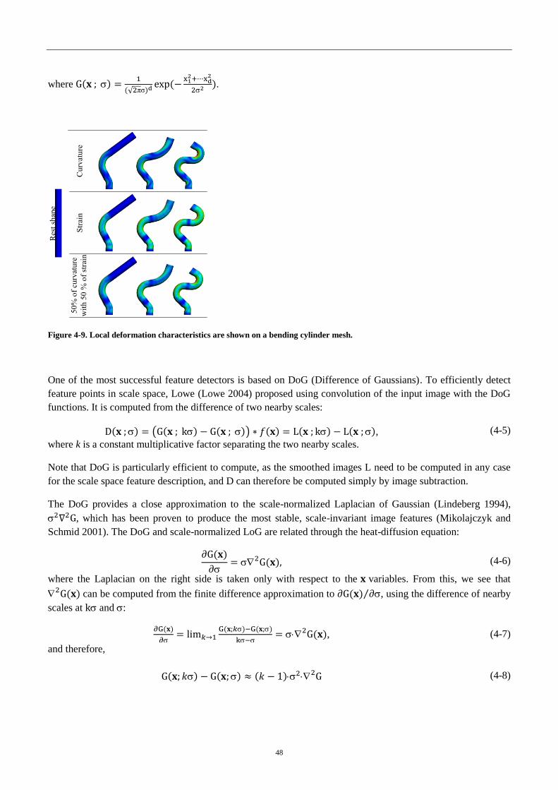
48

where

.

Res

t sh

ape

Cu

rvat

ure

S

trai

n

50

% o

f cu

rvat

ure

wit

h 5

0 %

of

stra

in

Figure 4-9. Local deformation characteristics are shown on a bending cylinder mesh.

One of the most successful feature detectors is based on DoG (Difference of Gaussians). To efficiently detect

feature points in scale space, Lowe (Lowe 2004) proposed using convolution of the input image with the DoG

functions. It is computed from the difference of two nearby scales:

, (4-5)

where k is a constant multiplicative factor separating the two nearby scales.

Note that DoG is particularly efficient to compute, as the smoothed images L need to be computed in any case

for the scale space feature description, and D can therefore be computed simply by image subtraction.

The DoG provides a close approximation to the scale-normalized Laplacian of Gaussian (Lindeberg 1994),

, which has been proven to produce the most stable, scale-invariant image features (Mikolajczyk and

Schmid 2001). The DoG and scale-normalized LoG are related through the heat-diffusion equation:

(4-6)

where the Laplacian on the right side is taken only with respect to the variables. From this, we see that

can be computed from the finite difference approximation to , using the difference of nearby

scales at and :

, (4-7)

and therefore,

(4-8)

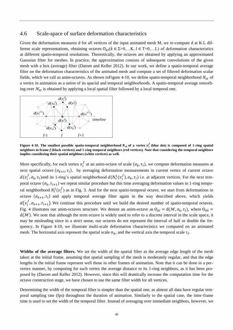
49

4.6 Scale-space of surface deformation characteristics

Given the deformation measures d for all vertices of the input animated mesh M, we re-compute d at K L dif-

ferent scale representations, obtaining octaves ( =0,…K, =0,…L) of deformation characteristics

at different spatio-temporal resolutions. Theoretically, the octaves are obtained by applying an approximated

Gaussian filter for meshes. In practice, the approximation consists of subsequent convolutions of the given

mesh with a box (average) filter (Darom and Keller 2012). In our work, we define a spatio-temporal average

filter on the deformation characteristics of the animated mesh and compute a set of filtered deformation scalar

fields, which we call as anim-octaves. As shown inFigure 4-10, we define spatio-temporal neighborhood of

a vertex in animation as a union of its spacial and temporal neighborhoods. A spatio-temporal average smooth-

ing over is obtained by applying a local spatial filter followed by a local temporal one.

timeline

d(vkf)

d(vjf)

d(vif+1

) d(vif-1

)

d(vif)

f-1 f+1 f

d(vlf)

d(vpf) d(vm

f)

Figure 4-10. The smallest possible spatio-temporal neighborhood of a vertex (blue dot) is composed of 1-ring spatial

neighbors in frame f (black vertices) and 1-ring temporal neighbors (red vertices). Note that considering the temporal neighbors

implies considering their spatial neighbors (white vertices) as well.

More specifically, for each vertex at an anim-octave of scale , we compute deformation measures at

next spatial octave , by averaging deformation measurements in current vertex of current octave

and its 1-ring’s spatial neighborhood

i.e. at adjacent vertices. For the next tem-

poral octave we repeat similar procedure but this time averaging deformation values in 1-ring tempo-

ral neighborhood

as in Fig. 3. And for the next spatio-temporal octave, we start from deformations in

octave and apply temporal average filter again in the way described above, which yields

We continue this procedure until we build the desired number of spatio-temporal octaves.

Fig. 4 illustrates our anim-octaves structure. We denote an anim-octave as , where

. We note that although the term octave is widely used to refer to a discrete interval in the scale space, it

may be misleading since in a strict sense, our octaves do not represent the interval of half or double the fre-

quency. In Figure 4-10, we illustrate multi-scale deformation characteristics we computed on an animated

mesh. The horizontal axis represent the spatial scale , and the vertical axis the temporal scale .

Widths of the average filters. We set the width of the spatial filter as the average edge length of the mesh

taken at the initial frame, assuming that spatial sampling of the mesh is moderately regular, and that the edge

lengths in the initial frame represent well those in other frames of animation. Note that it can be done in a per-

vertex manner, by computing for each vertex the average distance to its 1-ring neighbors, as it has been pro-

posed by (Darom and Keller 2012). However, since this will drastically increase the computation time for the

octave construction stage, we have chosen to use the same filter width for all vertices.

Determining the width of the temporal filter is simpler than the spatial one, as almost all data have regular tem-

poral sampling rate (fps) throughout the duration of animation. Similarly to the spatial case, the inter-frame

time is used to set the width of the temporal filter. Instead of averaging over immediate neighbors, however, we

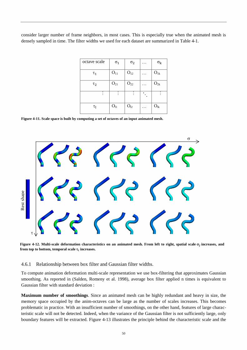
50

consider larger number of frame neighbors, in most cases. This is especially true when the animated mesh is

densely sampled in time. The filter widths we used for each dataset are summarized in Table 4-1.

octave scale

O11 O12 O1k

O21 O22 O2k

Ol1 Ol2 Olk

Figure 4-11. Scale space is built by computing a set of octaves of an input animated mesh.

Res

t sh

ape

Figure 4-12. Multi-scale deformation characteristics on an animated mesh. From left to right, spatial scale increases, and

from top to bottom, temporal scale increases.

4.6.1 Relationship between box filter and Gaussian filter widths.

To compute animation deformation multi-scale representation we use box-filtering that approximates Gaussian

smoothing. As reported in (Salden, Romeny et al. 1998), average box filter applied n times is equivalent to

Gaussian filter with standard deviation :

Maximum number of smoothings. Since an animated mesh can be highly redundant and heavy in size, the

memory space occupied by the anim-octaves can be large as the number of scales increases. This becomes

problematic in practice. With an insufficient number of smoothings, on the other hand, features of large charac-

teristic scale will not be detected. Indeed, when the variance of the Gaussian filter is not sufficiently large, only

boundary features will be extracted. Figure 4-13 illustrates the principle behind the characteristic scale and the

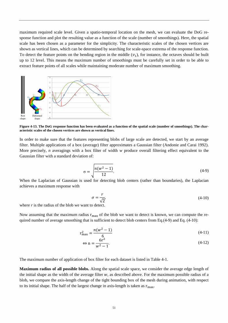
51

maximum required scale level. Given a spatio-temporal location on the mesh, we can evaluate the DoG re-

sponse function and plot the resulting value as a function of the scale (number of smoothings). Here, the spatial

scale has been chosen as a parameter for the simplicity. The characteristic scales of the chosen vertices are

shown as vertical lines, which can be determined by searching for scale-space extrema of the response function.

To detect the feature points on the bending region in the middle ( ), for instance, the octaves should be built

up to 12 level. This means the maximum number of smoothings must be carefully set in order to be able to

extract feature points of all scales while maintaining moderate number of maximum smoothing.

Rest

shape

Deformed

shape

v1 v2

v3

v1

v2

v3

Figure 4-13. The DoG response function has been evaluated as a function of the spatial scale (number of smoothings). The char-

acteristic scales of the chosen vertices are shown as vertical lines.

In order to make sure that the features representing blobs of large scale are detected, we start by an average

filter. Multiple applications of a box (average) filter approximates a Gaussian filter (Andonie and Carai 1992).

More precisely, n averagings with a box filter of width w produce overall filtering effect equivalent to the

Gaussian filter with a standard deviation of:

(4-9)

When the Laplacian of Gaussian is used for detecting blob centers (rather than boundaries), the Laplacian

achieves a maximum response with

(4-10)

where r is the radius of the blob we want to detect.

Now assuming that the maximum radius of the blob we want to detect is known, we can compute the re-

quired number of average smoothing that is sufficient to detect blob centers from Eq.(4-9) and Eq. (4-10):

(4-11)

(4-12)

The maximum number of application of box filter for each dataset is listed in Table 4-1.

Maximum radius of all possible blobs. Along the spatial scale space, we consider the average edge length of

the initial shape as the width of the average filter , as described above. For the maximum possible radius of a

blob, we compare the axis-length change of the tight bounding box of the mesh during animation, with respect

to its initial shape. The half of the largest change in axis-length is taken as .

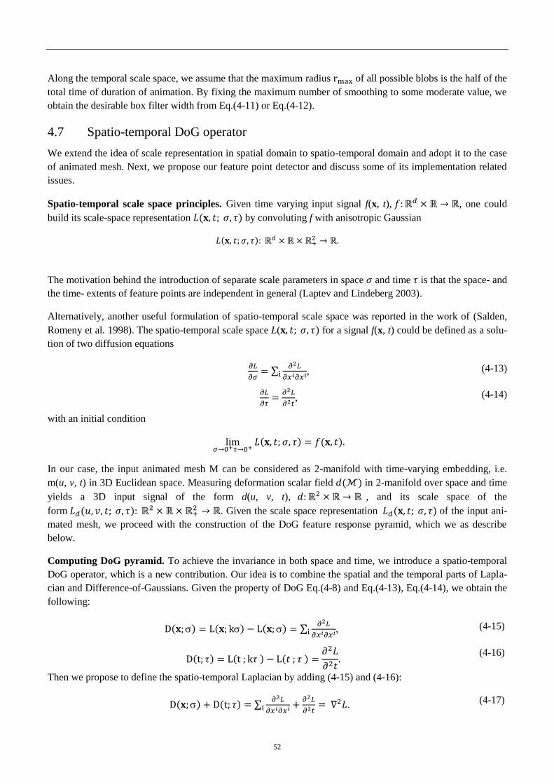
52

Along the temporal scale space, we assume that the maximum radius of all possible blobs is the half of the

total time of duration of animation. By fixing the maximum number of smoothing to some moderate value, we

obtain the desirable box filter width from Eq.(4-11) or Eq.(4-12).

4.7 Spatio-temporal DoG operator

We extend the idea of scale representation in spatial domain to spatio-temporal domain and adopt it to the case

of animated mesh. Next, we propose our feature point detector and discuss some of its implementation related

issues.

Spatio-temporal scale space principles. Given time varying input signal f(x, t), , one could

build its scale-space representation by convoluting f with anisotropic Gaussian

The motivation behind the introduction of separate scale parameters in space and time is that the space- and

the time- extents of feature points are independent in general (Laptev and Lindeberg 2003).

Alternatively, another useful formulation of spatio-temporal scale space was reported in the work of (Salden,

Romeny et al. 1998). The spatio-temporal scale space L( for a signal f(x, t) could be defined as a solu-

tion of two diffusion equations

, (4-13)

, (4-14)

with an initial condition

In our case, the input animated mesh M can be considered as 2-manifold with time-varying embedding, i.e.

m(u, v, t) in 3D Euclidean space. Measuring deformation scalar field in 2-manifold over space and time

yields a 3D input signal of the form d(u, v, t), , and its scale space of the

form

. Given the scale space representation of the input ani-

mated mesh, we proceed with the construction of the DoG feature response pyramid, which we as describe

below.

Computing DoG pyramid. To achieve the invariance in both space and time, we introduce a spatio-temporal

DoG operator, which is a new contribution. Our idea is to combine the spatial and the temporal parts of Lapla-

cian and Difference-of-Gaussians. Given the property of DoG Eq.(4-8) and Eq.(4-13), Eq.(4-14), we obtain the

following:

, (4-15)

(4-16)

Then we propose to define the spatio-temporal Laplacian by adding (4-15) and (4-16):

. (4-17)

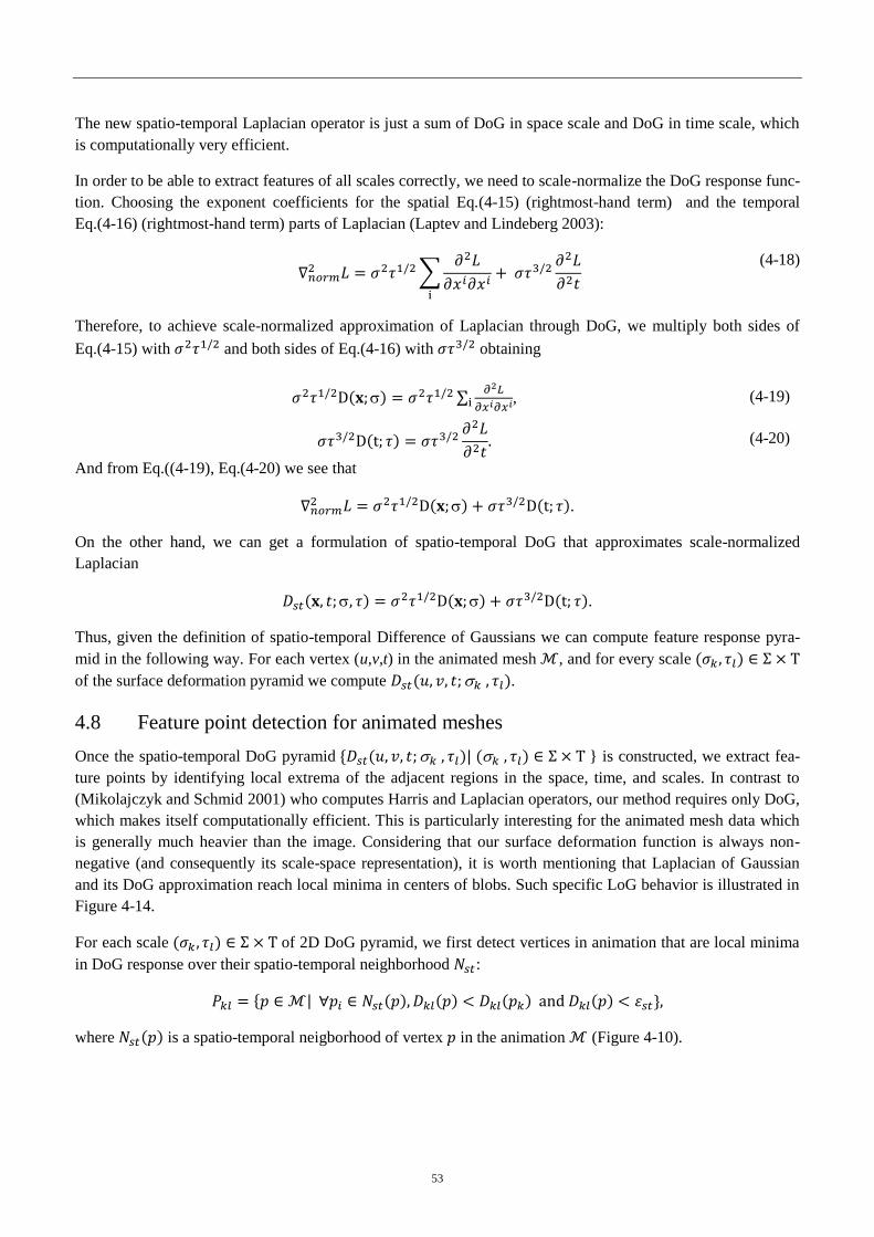
53

The new spatio-temporal Laplacian operator is just a sum of DoG in space scale and DoG in time scale, which

is computationally very efficient.

In order to be able to extract features of all scales correctly, we need to scale-normalize the DoG response func-

tion. Choosing the exponent coefficients for the spatial Eq.(4-15) (rightmost-hand term) and the temporal

Eq.(4-16) (rightmost-hand term) parts of Laplacian (Laptev and Lindeberg 2003):

(4-18)

Therefore, to achieve scale-normalized approximation of Laplacian through DoG, we multiply both sides of

Eq.(4-15) with and both sides of Eq.(4-16) with obtaining

, (4-19)

(4-20)

And from Eq.((4-19), Eq.(4-20) we see that

.

On the other hand, we can get a formulation of spatio-temporal DoG that approximates scale-normalized

Laplacian

.

Thus, given the definition of spatio-temporal Difference of Gaussians we can compute feature response pyra-

mid in the following way. For each vertex (u,v,t) in the animated mesh , and for every scale

of the surface deformation pyramid we compute .

4.8 Feature point detection for animated meshes

Once the spatio-temporal DoG pyramid } is constructed, we extract fea-

ture points by identifying local extrema of the adjacent regions in the space, time, and scales. In contrast to

(Mikolajczyk and Schmid 2001) who computes Harris and Laplacian operators, our method requires only DoG,

which makes itself computationally efficient. This is particularly interesting for the animated mesh data which

is generally much heavier than the image. Considering that our surface deformation function is always non-

negative (and consequently its scale-space representation), it is worth mentioning that Laplacian of Gaussian

and its DoG approximation reach local minima in centers of blobs. Such specific LoG behavior is illustrated in

Figure 4-14.

For each scale of 2D DoG pyramid, we first detect vertices in animation that are local minima

in DoG response over their spatio-temporal neighborhood :

where is a spatio-temporal neigborhood of vertex in the animation (Figure 4-10).

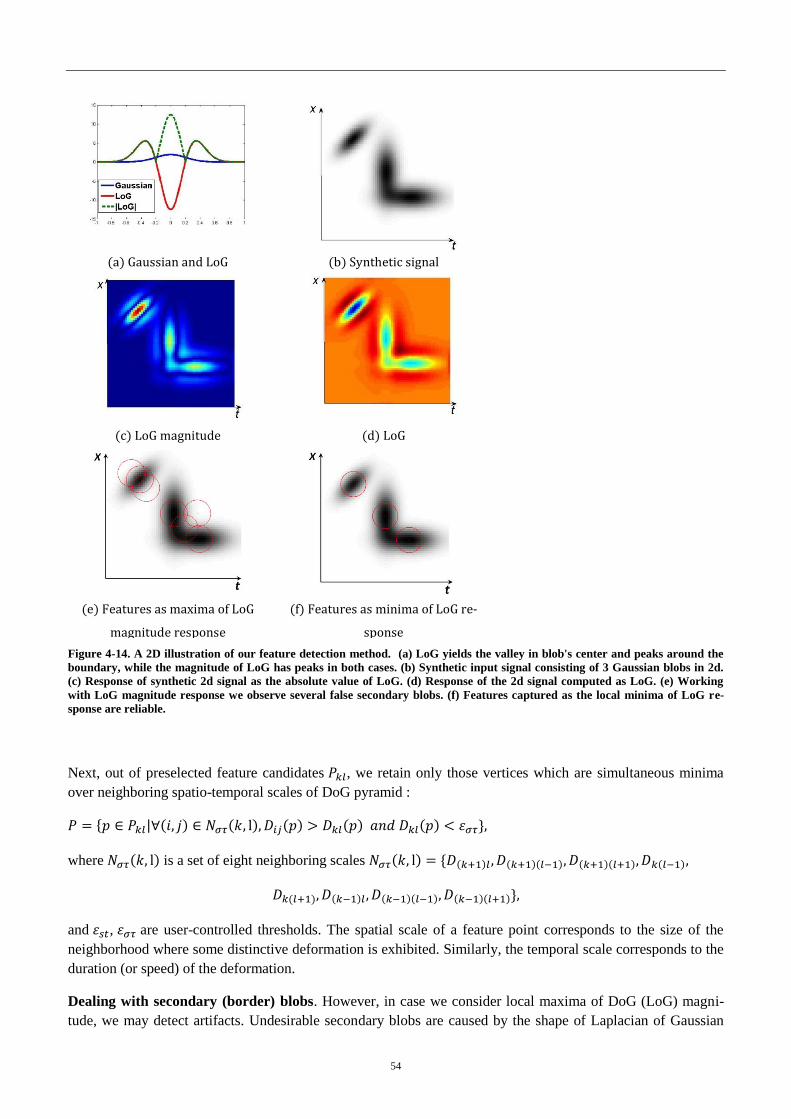
54

(a) Gaussian and LoG (b) Synthetic signal

(c) LoG magnitude (d) LoG

(e) Features as maxima of LoG

magnitude response

(f) Features as minima of LoG re-

sponse

Figure 4-14. A 2D illustration of our feature detection method. (a) LoG yields the valley in blob's center and peaks around the

boundary, while the magnitude of LoG has peaks in both cases. (b) Synthetic input signal consisting of 3 Gaussian blobs in 2d.

(c) Response of synthetic 2d signal as the absolute value of LoG. (d) Response of the 2d signal computed as LoG. (e) Working

with LoG magnitude response we observe several false secondary blobs. (f) Features captured as the local minima of LoG re-

sponse are reliable.

Next, out of preselected feature candidates , we retain only those vertices which are simultaneous minima

over neighboring spatio-temporal scales of DoG pyramid :

where is a set of eight neighboring scales

and , are user-controlled thresholds. The spatial scale of a feature point corresponds to the size of the

neighborhood where some distinctive deformation is exhibited. Similarly, the temporal scale corresponds to the

duration (or speed) of the deformation.

Dealing with secondary (border) blobs. However, in case we consider local maxima of DoG (LoG) magni-

tude, we may detect artifacts. Undesirable secondary blobs are caused by the shape of Laplacian of Gaussian

55

which yields peaks around the border of real blob (Figure 4-14(a)). Consider a perfect Gaussian blob as an in-

put signal. If we assume magnitude (i.e. absolute value) of LoG to be feature response, we get strong peak in

the center of the blob and two other secondary peaks around edges, and that is troublesome. In contrast, dealing

with signed LoG (not absolute) we observe valleys (local minima) in blob centers and peaks (local maxima) on

borders. Hence searching for local minima of LoG, rather than local maxima of LoG magnitude, prevents from

the detection of false secondary features Figure 4-14(b-f). The other way around could be to use LoG magni-

tude but discard local maxima which are not strong enough in initial signal, and therefore are false findings.

Though, previous works in feature extraction on images/video/static meshes (Mikolajczyk and Schmid 2001,

Laptev and Lindeberg 2003, Zaharescu, Boyer et al. 2009) often adopt Hessian detector, which does not detect

secondary blobs. However, in contrast to DoG detector, estimation of Hessian on a mesh surface is significantly

heavier. In the case of animated meshes estimation of Hessian matrix would me much more problematic and

computationally costly.

Implementation notes. Often, animated meshes are rather heavy data. As we increase the number of anim-

octaves in the pyramid, we can easily run out of memory, since each octave is essentially a full animation itself

but at different scale. Consequently, we have to address that issue in the implementation stage. In order to

minimize memory footprint, we compute pyramids and detect feature points progressively. We fully load into

main memory only space scale dimension of Gaussian and DoG pyramids. As for time scale, we keep only two

neighboring time octaves simultaneously, which are required for DoG computation. Then we construct the

pyramid from bottom to top by iteratively increasing time scale. On each iteration of Gausian/DoG pyramid

movement along time scale, we apply our feature detection method to capture interest points (if any on current

layer). We repeat the procedure until all pyramid scales have been processed.

4.9 Experiments

Deforming meshes used in our experiments include both synthetic animations and motion capture sequences,

which are summarized in Table 3-1. We synthesized a simple deforming Cylinder animation by rigging and

used it for initial tests. Also we captured two person’s facial expressions using Vicon system (Vicon) and then

transferred the expressions to the scanned faces of the two persons Face1 and Face2.

Name No.vertices/

triangles

No. frames Filter widths (space/time) Max. no. smoothings

(space/time) Cylinder 587/1170 40 10.0/0.83 50/100

Face1(happy) 608/1174 139 8.96/8.45 118/113

Face1(surprise) 608/1174 169 9.39/13.2 96/107

Face2(happy) 662/1272 159 9.31/13.2 112/94

Face2(surprise) 662/1272 99 8.95/8.45 109/57

Horse 5000/9984 48 3.48/5.33 77/54

Camel 4999/10000 48 2.62/5.33 102/54

Woman1 4250/8476 100 5.12/5.2 72/150

Woman2 4250/8476 100 4.44/5.2 82/150

Woman3 4250/8476 100 4.54/5.2 99/150

Face3 5192/9999 71 5.18/3.65 90/114

Head 7966/15809 71 9.06/3.65 28/114

Table 4-1. The animated meshes used in our experiments.

Figure 4-15 shows selected frames of several animated meshes we used in our experiments. Spatio-temporal

feature points we have extracted using our algorithm are illustrated as spheres. The demo video that is available

56

at https://vimeo.com/120707827 shows the complete animation sequences along with the extracted dynamic

feature points.

Face1 (happy), Face1 (surprise), Face2 (happy), Face2 (surprise) contain facial expressions of happiness and

surprise of those scanned subjects. The horse and the camel were obtained from results of (Sumner and Popović

2004) work. Furthermore, we produced two mesh animations of seventy frames, Face3 and Head, by using nine

facial expressions of the face and the head from (Sumner and Popović 2004). More specifically, given an or-

dered sequence of nine facial expressions, we smoothly morphed each mesh to the next one through a linear

interpolation of their vertex coordinates. We also used skeletal animations of three women models performing

“walk and whirl” motions. Those models share the same mesh connectivity and were obtained by deforming a

template mesh onto three body scans of different subjects. Note that there is high semantic similarity between

animation pairs of Face1/Face2, horse/camel, Face3/Head. It is also the case for three women models.

The color of a sphere represents the temporal scale (red color corresponds to more fast deformations) of the

feature point, and radius of sphere indicates the spatial scale. Vertex color on surfaces corresponds to amount of

deformation (strain and curvature change) observed in each of animation frame. During experiments we have

discovered that our method captures spatio-temporal scales in a robust manner. For example, surface patches

around joints of cylinder (Figure 4-16 1a-1e) exhibit different amount of deformation that occurs at different

speed. The top joint is moving fast and consequently corresponding feature was detected at low temporal scale

(red color). However, the mid-joint is deforming for a long time and we identify it at high temporal scale (blue

color). Moreover large radii of deforming spheres for both joints make sense and indicate large deforming re-

gions around the features, rather than very local deformation (Figure 4-16 1c). Second row in (Figure 4-16 2a-

2e) depicts some of the feature points in the galloping Horse mesh animation, and third row (Figure 4-16 3a-3e)

corresponds to the galloping Camel animation. Those two meshes deform in a coherent manner (Sumner and

Popović 2004), and eventually we detect their spatio-temporal features quite consistently. In the last two rows

(Figure 4-16 4a-4e, 5a-5e) we present feature points in mocap-driven face animations of two different subjects.

Our subjects were asked to mimic of slightly exaggerated emotions during the mocap session. Notice that peo-

ple normally use different set of muscles when they show up facial expressions, and therefore naturally we

observe some variations in the way their skin deforms.

Our algorithm is implemented in C++. All our tests have been conducted on an Intel Core i7–2600 3.4 GHz

machine, with 8GB of RAM. The computation time devoted to full pipeline of the algorithm is approximately 2

minutes for most of our example data.

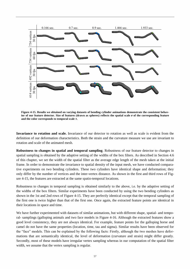
57

734 v

erti

ces

30 f

ps

0.166 sec. 0.7 sec. 0.9 sec. 1.466 sec. 1.933 sec. 734 v

erti

ces

60 f

ps

492 v

erti

ces

30 f

ps

614 v

erti

ces

30 f

ps

Figure 4-15. Results we obtained on varying datasets of bending cylinder animations demonstrate the consistent behav-

ior of our feature detector. Size of features (drawn as spheres) reflects the spatial scale of the corresponding feature

and the color corresponds to temporal scale .

Invariance to rotation and scale. Invariance of our detector to rotation as well as scale is evident from the

definition of our deformation characteristics. Both the strain and the curvature measure we use are invariant to

rotation and scale of the animated mesh.

Robustness to changes in spatial and temporal sampling. Robustness of our feature detector to changes in

spatial sampling is obtained by the adaptive setting of the widths of the box filters. As described in Section 4.6

of this chapter, we set the width of the spatial filter as the average edge length of the mesh taken at the initial

frame. In order to demonstrate the invariance to spatial density of the input mesh, we have conducted compara-

tive experiments on two bending cylinders. These two cylinders have identical shape and deformation; they

only differ by the number of vertices and the inter-vertex distance. As shown in the first and third rows of Fig-

ure 4-15, the features are extracted at the same spatio-temporal locations.

Robustness to changes in temporal sampling is obtained similarly to the above, i.e. by the adaptive setting of

the widths of the box filters. Similar experiments have been conducted by using the two bending cylinders as

shown in the 1st and 2nd rows of Figure 4-15. They are perfectly identical except that the temporal sampling of

the first one is twice higher than that of the first one. Once again, the extracted feature points are identical in

their locations in space and time.

We have further experimented with datasets of similar animations, but with different shape, spatial- and tempo-

ral- samplings (galloping animals and two face models in Figure 4-16. Although the extracted features show a

good level consistency, they are not always identical. For example, feature points for the galloping horse and

camel do not have the same properties (location, time, tau and sigma). Similar results have been observed for

the “face” models. This can be explained by the following facts: Firstly, although the two meshes have defor-

mations that are semantically identical, the level of deformation (curvature and strain) might differ greatly.

Secondly, most of these models have irregular vertex sampling whereas in our computation of the spatial filter

width, we assume that the vertex sampling is regular.

58

Figure 4-16. Dynamic feature points detected by our AniM-DoG framework are illustrated on a number of selected frames of

animated meshes. The color of a sphere represents the temporal scale (from blue to red) of the feature point, and radius of sphere

indicates the spacial scale.

4.9.1 Consistency

Since our method is based on deformation characteristics, it has an advantage of consistent feature point extrac-

tion across mesh animations with similar motions. To demonstrate mutual consistency among feature points in

different animations, we used animation data that exhibit semantically similar motions. Our technique captures

similarity of surface deformations and therefore ensures feature point detection consistency (Figure 4-17).

(1a) (1b) (1c) (1d) (1e)

(2a) (2b) (2c) (2d) (2e)

(3a) (3b) (3c) (3d) (3e)

(4a) (4b) (4c) (4d) (4e)

(5a) (5b) (5c) (5d) (5e)

59

#frame 11 #frame 13 #frame 18 #frame 33 #frame 77

(a)

(b)

#frame 10 #frame 20 #frame 22 #frame 30 #frame 50

(c)

(d)

Figure 4-17. Inter-subject consistency of feature points extracted from semantically similar mesh animations. Rows (a-b) depict

subset of feature points extracted from walking subject sequences (woman2/woman3 as in Table 4-1) and (c-d) from Face3/Head

animations. Note that each column corresponds to identical frame of the animations.

In most cases our method demonstrates high coherency not only in space and time locations of extracted fea-

tures but also in their space-time scales and . The only data sets for which we observed relatively lower con-

sistency of feature detection are the two face mocap sequences. The reason for this lies in inherent difference of

people’s facial expressions and underlying muscle anatomy.

Additionally, we have performed the quantitative evaluation of the feature extraction consistency as follows.

For all feature points we consider only their spatial locations disregarding the time coordinates. Then a pair of

similarly deforming meshes and whose full correspondence is known, we find the match-

ing between their feature points and based on the spatial proximity. More precisely, for each feature point

, the feature point

that minimizes

is considered to be the matching one. The

distance is what we call feature matching error. Histogram plots of feature matching errors are depicted in

Figure 4-18. Obtaining the full correspondence for walking women models was straightforward because they

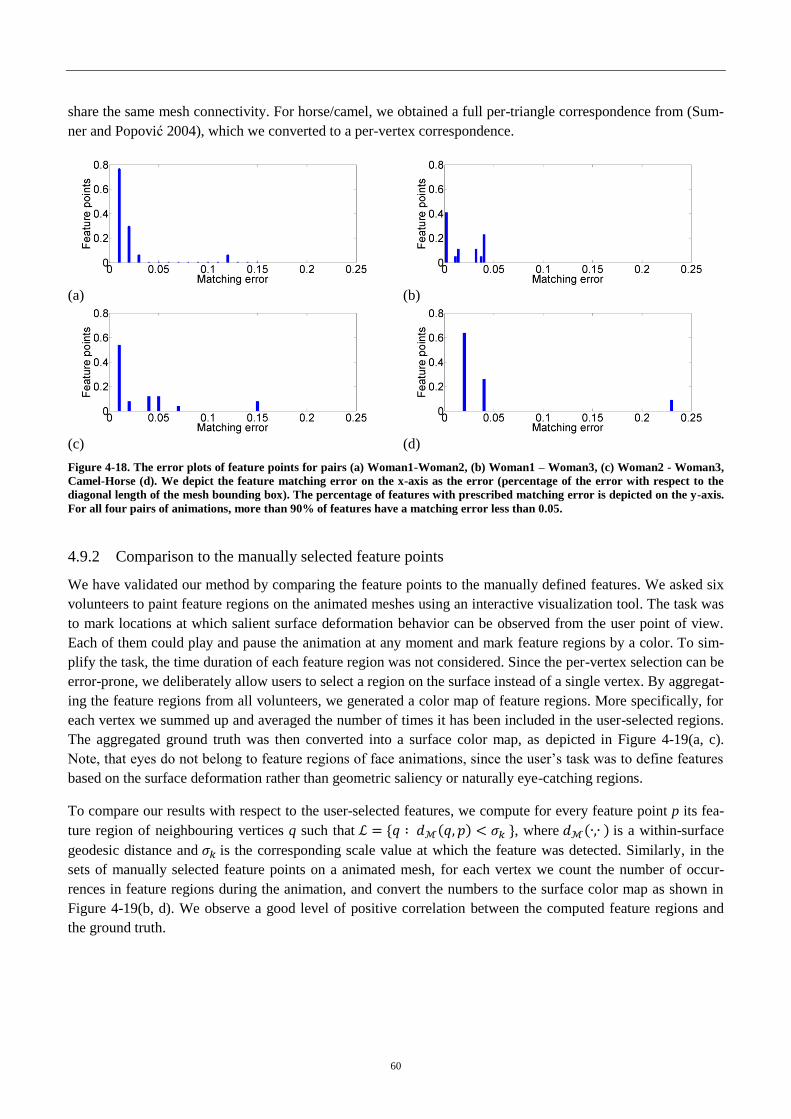
60

share the same mesh connectivity. For horse/camel, we obtained a full per-triangle correspondence from (Sum-

ner and Popović 2004), which we converted to a per-vertex correspondence.

(a) (b)

(c) (d)

Figure 4-18. The error plots of feature points for pairs (a) Woman1-Woman2, (b) Woman1 – Woman3, (c) Woman2 - Woman3,

Camel-Horse (d). We depict the feature matching error on the x-axis as the error (percentage of the error with respect to the

diagonal length of the mesh bounding box). The percentage of features with prescribed matching error is depicted on the y-axis.

For all four pairs of animations, more than 90% of features have a matching error less than 0.05.

4.9.2 Comparison to the manually selected feature points

We have validated our method by comparing the feature points to the manually defined features. We asked six

volunteers to paint feature regions on the animated meshes using an interactive visualization tool. The task was

to mark locations at which salient surface deformation behavior can be observed from the user point of view.

Each of them could play and pause the animation at any moment and mark feature regions by a color. To sim-

plify the task, the time duration of each feature region was not considered. Since the per-vertex selection can be

error-prone, we deliberately allow users to select a region on the surface instead of a single vertex. By aggregat-

ing the feature regions from all volunteers, we generated a color map of feature regions. More specifically, for

each vertex we summed up and averaged the number of times it has been included in the user-selected regions.

The aggregated ground truth was then converted into a surface color map, as depicted in Figure 4-19(a, c).

Note, that eyes do not belong to feature regions of face animations, since the user’s task was to define features

based on the surface deformation rather than geometric saliency or naturally eye-catching regions.

To compare our results with respect to the user-selected features, we compute for every feature point p its fea-

ture region of neighbouring vertices q such that , where is a within-surface

geodesic distance and is the corresponding scale value at which the feature was detected. Similarly, in the

sets of manually selected feature points on a animated mesh, for each vertex we count the number of occur-

rences in feature regions during the animation, and convert the numbers to the surface color map as shown in

Figure 4-19(b, d). We observe a good level of positive correlation between the computed feature regions and

the ground truth.

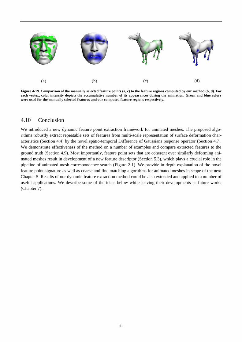
61

(a) (b) (c) (d)

Figure 4-19. Comparison of the manually selected feature points (a, c) to the feature regions computed by our method (b, d). For

each vertex, color intensity depicts the accumulative number of its appearances during the animation. Green and blue colors

were used for the manually selected features and our computed feature regions respectively.

4.10 Conclusion

We introduced a new dynamic feature point extraction framework for animated meshes. The proposed algo-

rithms robustly extract repeatable sets of features from multi-scale representation of surface deformation char-

acteristics (Section 4.4) by the novel spatio-temporal Difference of Gaussians response operator (Section 4.7).

We demonstrate effectiveness of the method on a number of examples and compare extracted features to the

ground truth (Section 4.9). Most importantly, feature point sets that are coherent over similarly deforming ani-

mated meshes result in development of a new feature descriptor (Section 5.3), which plays a crucial role in the

pipeline of animated mesh correspondence search (Figure 2-1). We provide in-depth explanation of the novel

feature point signature as well as coarse and fine matching algorithms for animated meshes in scope of the next

Chapter 5. Results of our dynamic feature extraction method could be also extended and applied to a number of

useful applications. We describe some of the ideas below while leaving their developments as future works

(Chapter 7).

62

Chapter 5 Correspondence between animated

meshes

5.1 Introduction

In Chapter 4 we presented a novel method for a dynamic feature point extraction which is initial and very im-

portant stage in scope of our shape correspondence framework for animated meshes. In Chapter 5 we focus on

how dynamic feature points can be incorporated in a complete animated shape correspondence framework.

If we want to move towards shape correspondence techniques capable of exploiting rich set of information on

dynamic images, we have to put an entirely new perspective on the traditional shape correspondence pipeline,

trying to understand where and how the mobility can be encapsulated. To reach this objective, we will focus on

the following questions: - How to efficiently represent the movement data from the dynamic images, and at

different stages of shape correspondence? - How to interpret the movement data towards finding reliable corre-

spondence?

This chapter details the new method of animated mesh matching. The main difference of our method to existing

approaches is that it makes use of dynamic properties of animated mesh rather than on its static geometry. In

scope of this chapter we develop a novel dynamic point descriptor that serves as a robust signature for the dy-

namic features. Given the similarity measure between the dynamic feature point descriptors, we approach the

animated mesh matching by first computing sparse matching of dynamic features followed by full matching of

every vertex of the source and target animations.

The pipeline of the proposed technique consists of several major substeps. The initial step (Figure 5-1(1)) of

dynamic feature extraction from an animated mesh is detailed in Chapter 4. Then each feature on the source

and target is supplied with the dynamic feature point descriptor (Figure 5-1(2)), and followed by sparse feature

correspondence (Figure 5-1(3)) and dense full mesh correspondence (Figure 5-1(4)). This chapter is organized

as follows. First, we detail our new feature point signature that is able to not only robustly capture dynamic

motion properties of features, but also effectively used for feature matching. Based on these feature point de-

scriptors we propose to compute initial sparse correspondences of dynamic feature points using dual decompo-

sition graph matching technique (Torresani, Kolmogorov et al. 2008). Then we overview the core aspects of

our graph matching approach and show its robustness in feature matching.

Finally, we develop a new dense correspondence (full matching) approach between the source and the target

meshes in spherical embedding. Full matching in spherical parameterization is formulated as a sequence of

warping in spherical domain that optimally align initial sparse correspondences of dynamic features.

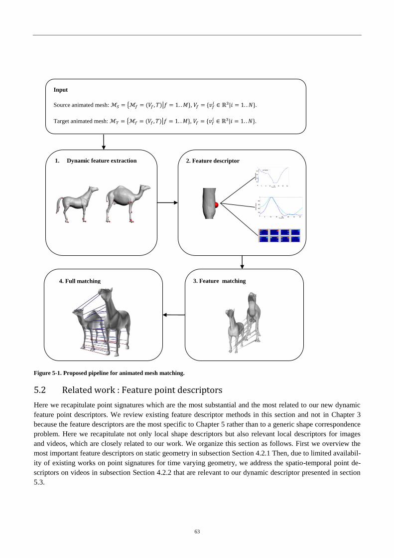
63

Figure 5-1. Proposed pipeline for animated mesh matching.

5.2 Related work : Feature point descriptors

Here we recapitulate point signatures which are the most substantial and the most related to our new dynamic

feature point descriptors. We review existing feature descriptor methods in this section and not in Chapter 3

because the feature descriptors are the most specific to Chapter 5 rather than to a generic shape correspondence

problem. Here we recapitulate not only local shape descriptors but also relevant local descriptors for images

and videos, which are closely related to our work. We organize this section as follows. First we overview the

most important feature descriptors on static geometry in subsection Section 4.2.1 Then, due to limited availabil-

ity of existing works on point signatures for time varying geometry, we address the spatio-temporal point de-

scriptors on videos in subsection Section 4.2.2 that are relevant to our dynamic descriptor presented in section

5.3.

Input

Source animated mesh: , .

Target animated mesh: , .

1. Dynamic feature extraction

2. Feature descriptor

4. Full matching 3. Feature matching

64

5.2.1 Spatial feature descriptors for surface matching

A vast variety of point signatures and feature descriptors has been proposed in the literature for the 3d geometry

(Johnson 1997, Gatzke, Grimm et al. 2005, Gelfand, Mitra et al. 2005, Castellani, Cristani et al. 2008, Sun,

Ovsjanikov et al. 2009, Zaharescu, Boyer et al. 2009, Tevs, Berner et al. 2011, Darom and Keller 2012). Here

we describe each of the most important shape descriptors. Note that we focus on the local shape descriptors

since the global descriptors are not directly relevant to our work. Most of the common low dimensional shape

descriptors rely on differential quantities of the shape that makes them sensitive to noise in the input data.

Therefore in order to make differential shape descriptors useful for the shape correspondence, in most of the

cases data smoothing has to be performed.

Spin image is one of the first surface shape descriptors originally proposed by (Johnson 1997). The spin image

surface representation technique is often used for surface matching and object recognition in 3-D scenes. Spin

images essentially encode the global properties of a given surface in an object-oriented coordinate system. Spin

image (or spin map) is a 2d histogram of point locations accumulated in cylindrical coordinates (aligned as the

point’s normal) over the surface’s locale support region. Each point within the local support region is projected

into corresponding bin depending on its cylindrical coordinates. The procedure is repeated for all vertices

within the support region of the spin image. The resulting accumulation spin map can be thought of as a 2D

image (Figure 5-2).

Scale-invariant spin image (SISI). Scale-invariant spin image (SISI) descriptor for meshes (Darom and Keller

2012) extends classical spin image shape descriptor (Johnson 1997). The computation of the original spin im-

age descriptor (Johnson 1997) relies on a constant predefined support in a neighborhood of a point, hence it is

rather global in nature. Therefore in a recent work of (Darom and Keller 2012) the authors propose to compute

the scale-invariant version of spin image (SISI) by computing the descriptor over the adaptive local scale that

corresponds to the scale at which a feature was detected (Darom and Keller 2012).

Figure 5-2. Spin image shape descriptor (Johnson 1997). Dark areas in the image correspond to bins that contain many accumu-

lated points.

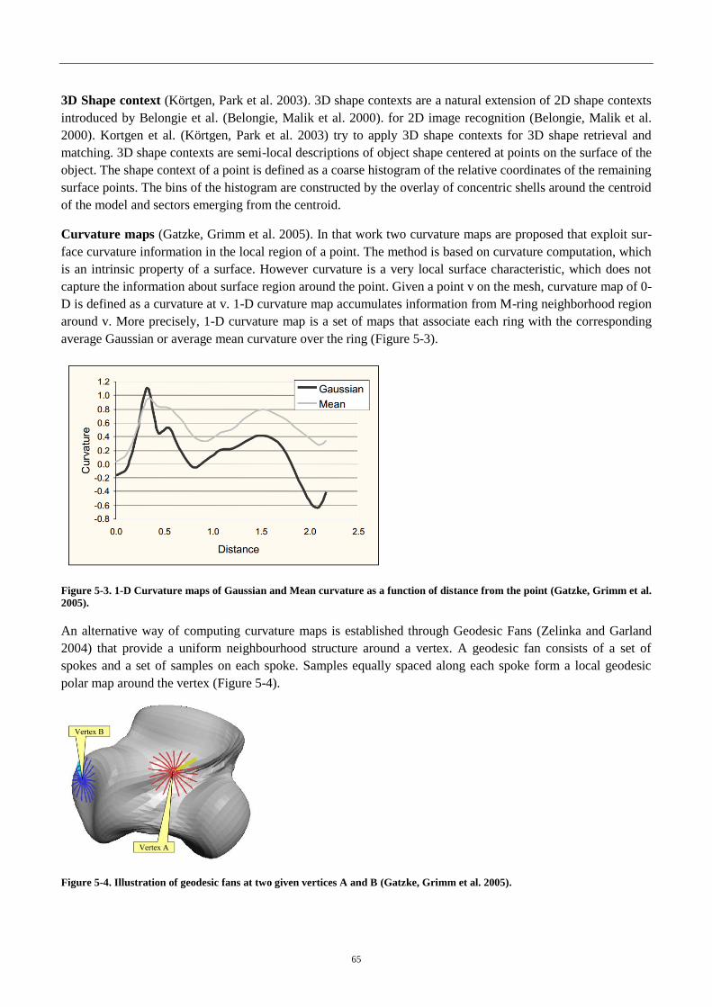
65

3D Shape context (Körtgen, Park et al. 2003). 3D shape contexts are a natural extension of 2D shape contexts

introduced by Belongie et al. (Belongie, Malik et al. 2000). for 2D image recognition (Belongie, Malik et al.

2000). Kortgen et al. (Körtgen, Park et al. 2003) try to apply 3D shape contexts for 3D shape retrieval and

matching. 3D shape contexts are semi-local descriptions of object shape centered at points on the surface of the

object. The shape context of a point is defined as a coarse histogram of the relative coordinates of the remaining

surface points. The bins of the histogram are constructed by the overlay of concentric shells around the centroid

of the model and sectors emerging from the centroid.

Curvature maps (Gatzke, Grimm et al. 2005). In that work two curvature maps are proposed that exploit sur-

face curvature information in the local region of a point. The method is based on curvature computation, which

is an intrinsic property of a surface. However curvature is a very local surface characteristic, which does not

capture the information about surface region around the point. Given a point v on the mesh, curvature map of 0-

D is defined as a curvature at v. 1-D curvature map accumulates information from M-ring neighborhood region

around v. More precisely, 1-D curvature map is a set of maps that associate each ring with the corresponding

average Gaussian or average mean curvature over the ring (Figure 5-3).

Figure 5-3. 1-D Curvature maps of Gaussian and Mean curvature as a function of distance from the point (Gatzke, Grimm et al.

2005).

An alternative way of computing curvature maps is established through Geodesic Fans (Zelinka and Garland

2004) that provide a uniform neighbourhood structure around a vertex. A geodesic fan consists of a set of

spokes and a set of samples on each spoke. Samples equally spaced along each spoke form a local geodesic

polar map around the vertex (Figure 5-4).

Figure 5-4. Illustration of geodesic fans at two given vertices A and B (Gatzke, Grimm et al. 2005).

66

Given a geodesic fan computed around vertex v, instead of ring-based 1-D Curvature map it is possible to de-

fine a fan-based curvature map. For that, each spoke of the fan is associated with a function of Gaussian/mean

curvature as a function of distance from the point v. 2-D curvature map is defined similarly to 1-D map, except

that angular information (i.e. angle between normals of sample points) is kept along the spoke of the fan. Addi-

tionally (Gatzke, Grimm et al. 2005) show that curvature maps are robust to mesh resolution and regularity.

Integral descriptor (Gelfand, Mitra et al. 2005). Gelfand et al. proposed an Integral Volume local shape de-

scriptor. The descriptor is robust to geometric noise and is invariant under rigid transformations, which makes it

useful for shape correspondence algorithms. The Integral Volume descriptor is defined at each point p of the

shape as

. Where the integral kernel corresponds to the ball of the radius r centered

at p, and S is the interior of the surface at p (Figure 5-5). In practice the integral

is computed over

discrete voxel grid as depicted in Figure 5-5 (b). The authors demonstrate the Integral Volume descriptor is

closely related to the mean curvature H of the surface, but in contrast to H much more robust to the noise.

Figure 5-5. 2D analogy of the Integral Volume descriptor (Gelfand, Mitra et al. 2005). (a) The Integral Volume descriptor

measures the volume of the ball of radius r centered at point p defined by the local interior of the shape. (b) is computed

in discrete voxel grid.

Statistical descriptor. In the work of (Castellani, Cristani et al. 2008), the authors propose a feature descriptor

that relies on statistical Hidden Markov Model (Rabiner 1989) to collect the information related the feature

point and its neighborhood. Given a feature point p, a clockwise spiral path is constructed on the surface around

p until a fixed geodesic radius is reached (Figure 5-6). Along the spiral the following five entities are sampled:

local point information (Petitjean 2002), saliency level (Castellani, Cristani et al. 2008), maximal curvature,

minimal curvature, normal displacement between local point and the feature p. These repeatedly occurring 5-

dimensional entries can be modeled as a stochastic process by discrete HMM (Rabiner 1989). In such a way,

HMM descriptor gives a statistical encoding of the interest point and its neighborhood. For measuring similari-

ties between HMM descriptors of different features a classical HMM similarity measure (Smyth 1997) can be

successfully used. The matching of features based on HMM descriptor shows robust and accurate results for the

rigid partially incomplete shapes (Castellani, Cristani et al. 2008).

MeshHoG (Mesh Histogram of Oriented Gradients). (Zaharescu, Boyer et al. 2009) propose an extension of

the Histogram of Oriented Gradients method of (Dalal and Triggs 2005) from the image domain to the domain

of 3D meshes. Given vertex , the descriptor relies on the information gathered within support region of

size r around . The size of the support region is chosen adaptively depending on a given mesh in a way that r

is proportional to the square root of the mesh area and inversely proportional to the average edge length

. More precisely, given the user parameter , the value of is computed as following

.Then 3D discrete gradients of the photometric data of the mesh in the neighborhood are

pooled into a polar histogram . Given the dominant orientation in the histogram and normal vector

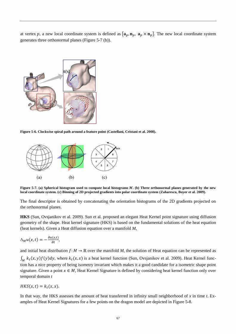
67

at vertex , a new local coordinate system is defined as . The new local coordinate system

generates three orthonormal planes (Figure 5-7 (b)).

Figure 5-6. Clockwise spiral path around a feature point (Castellani, Cristani et al. 2008).

Figure 5-7. (a) Spherical histogram used to compute local histograms . (b) Three orthonormal planes generated by the new

local coordinate system. (c) Binning of 2D projected gradients into polar coordinate system (Zaharescu, Boyer et al. 2009).

The final descriptor is obtained by concatenating the orientation histograms of the 2D gradients projected on

the orthonormal planes.

HKS (Sun, Ovsjanikov et al. 2009). Sun et al. proposed an elegant Heat Kernel point signature using diffusion

geometry of the shape. Heat kernel signature (HKS) is based on the fundamental solutions of the heat equation

(heat kernels). Given a Heat diffusion equation over a manifold M,

,

and initial heat distribution over the manifold M, the solution of Heat equation can be represented as

, where is a heat kernel function (Sun, Ovsjanikov et al. 2009). Heat Kernel func-

tion has a nice property of being isometry invariant which makes it a good candidate for a isometric shape point

signature. Given a point , Heat Kernel Signature is defined by considering heat kernel function only over

temporal domain t

.

In that way, the HKS assesses the amount of heat transferred in infinity small neighborhood of x in time t. Ex-

amples of Heat Kernel Signatures for a few points on the dragon model are depicted in Figure 5-8.

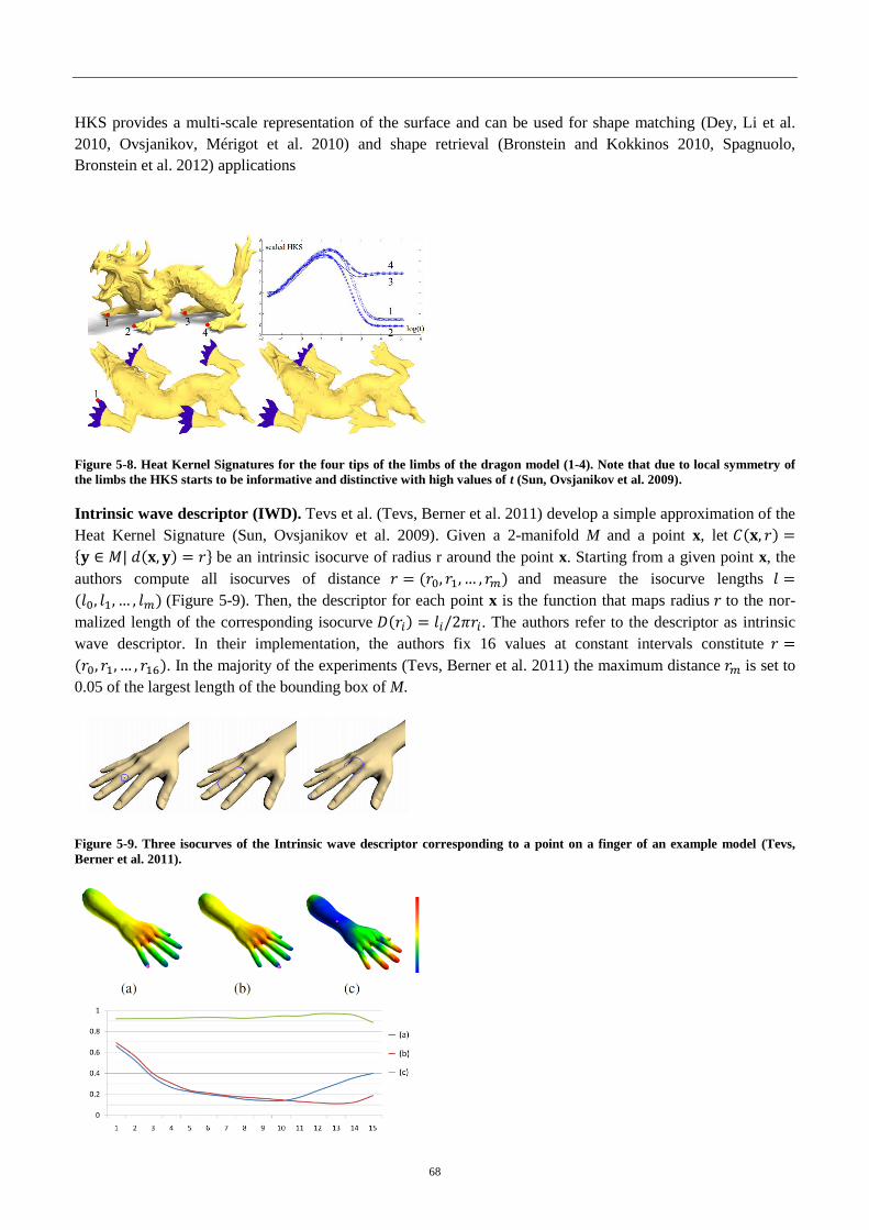
68

HKS provides a multi-scale representation of the surface and can be used for shape matching (Dey, Li et al.

2010, Ovsjanikov, Mérigot et al. 2010) and shape retrieval (Bronstein and Kokkinos 2010, Spagnuolo,

Bronstein et al. 2012) applications

Figure 5-8. Heat Kernel Signatures for the four tips of the limbs of the dragon model (1-4). Note that due to local symmetry of

the limbs the HKS starts to be informative and distinctive with high values of t (Sun, Ovsjanikov et al. 2009).

Intrinsic wave descriptor (IWD). Tevs et al. (Tevs, Berner et al. 2011) develop a simple approximation of the

Heat Kernel Signature (Sun, Ovsjanikov et al. 2009). Given a 2-manifold M and a point x, let

be an intrinsic isocurve of radius r around the point x. Starting from a given point x, the

authors compute all isocurves of distance and measure the isocurve lengths

(Figure 5-9). Then, the descriptor for each point x is the function that maps radius to the nor-

malized length of the corresponding isocurve . The authors refer to the descriptor as intrinsic

wave descriptor. In their implementation, the authors fix 16 values at constant intervals constitute

. In the majority of the experiments (Tevs, Berner et al. 2011) the maximum distance is set to

0.05 of the largest length of the bounding box of M.

Figure 5-9. Three isocurves of the Intrinsic wave descriptor corresponding to a point on a finger of an example model (Tevs,

Berner et al. 2011).

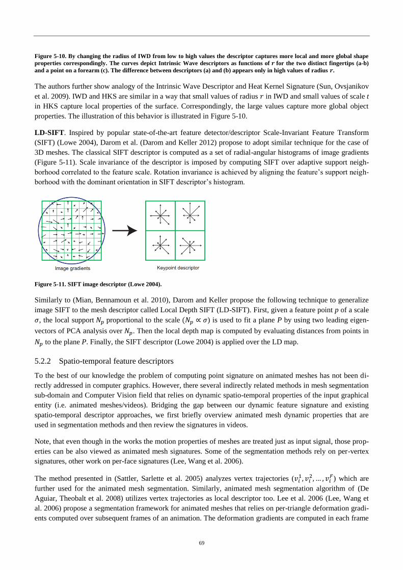
69

Figure 5-10. By changing the radius of IWD from low to high values the descriptor captures more local and more global shape

properties correspondingly. The curves depict Intrinsic Wave descriptors as functions of for the two distinct fingertips (a-b)

and a point on a forearm (c). The difference between descriptors (a) and (b) appears only in high values of radius .

The authors further show analogy of the Intrinsic Wave Descriptor and Heat Kernel Signature (Sun, Ovsjanikov

et al. 2009). IWD and HKS are similar in a way that small values of radius in IWD and small values of scale t

in HKS capture local properties of the surface. Correspondingly, the large values capture more global object

properties. The illustration of this behavior is illustrated in Figure 5-10.

LD-SIFT. Inspired by popular state-of-the-art feature detector/descriptor Scale-Invariant Feature Transform

(SIFT) (Lowe 2004), Darom et al. (Darom and Keller 2012) propose to adopt similar technique for the case of

3D meshes. The classical SIFT descriptor is computed as a set of radial-angular histograms of image gradients

(Figure 5-11). Scale invariance of the descriptor is imposed by computing SIFT over adaptive support neigh-

borhood correlated to the feature scale. Rotation invariance is achieved by aligning the feature’s support neigh-

borhood with the dominant orientation in SIFT descriptor’s histogram.

Figure 5-11. SIFT image descriptor (Lowe 2004).

Similarly to (Mian, Bennamoun et al. 2010), Darom and Keller propose the following technique to generalize

image SIFT to the mesh descriptor called Local Depth SIFT (LD-SIFT). First, given a feature point p of a scale

, the local support proportional to the scale ) is used to fit a plane P by using two leading eigen-

vectors of PCA analysis over . Then the local depth map is computed by evaluating distances from points in

to the plane P. Finally, the SIFT descriptor (Lowe 2004) is applied over the LD map.

5.2.2 Spatio-temporal feature descriptors

To the best of our knowledge the problem of computing point signature on animated meshes has not been di-

rectly addressed in computer graphics. However, there several indirectly related methods in mesh segmentation

sub-domain and Computer Vision field that relies on dynamic spatio-temporal properties of the input graphical

entity (i.e. animated meshes/videos). Bridging the gap between our dynamic feature signature and existing

spatio-temporal descriptor approaches, we first briefly overview animated mesh dynamic properties that are

used in segmentation methods and then review the signatures in videos.

Note, that even though in the works the motion properties of meshes are treated just as input signal, those prop-

erties can be also viewed as animated mesh signatures. Some of the segmentation methods rely on per-vertex

signatures, other work on per-face signatures (Lee, Wang et al. 2006).

The method presented in (Sattler, Sarlette et al. 2005) analyzes vertex trajectories (

) which are

further used for the animated mesh segmentation. Similarly, animated mesh segmentation algorithm of (De

Aguiar, Theobalt et al. 2008) utilizes vertex trajectories as local descriptor too. Lee et al. 2006 (Lee, Wang et

al. 2006) propose a segmentation framework for animated meshes that relies on per-triangle deformation gradi-

ents computed over subsequent frames of an animation. The deformation gradients are computed in each frame

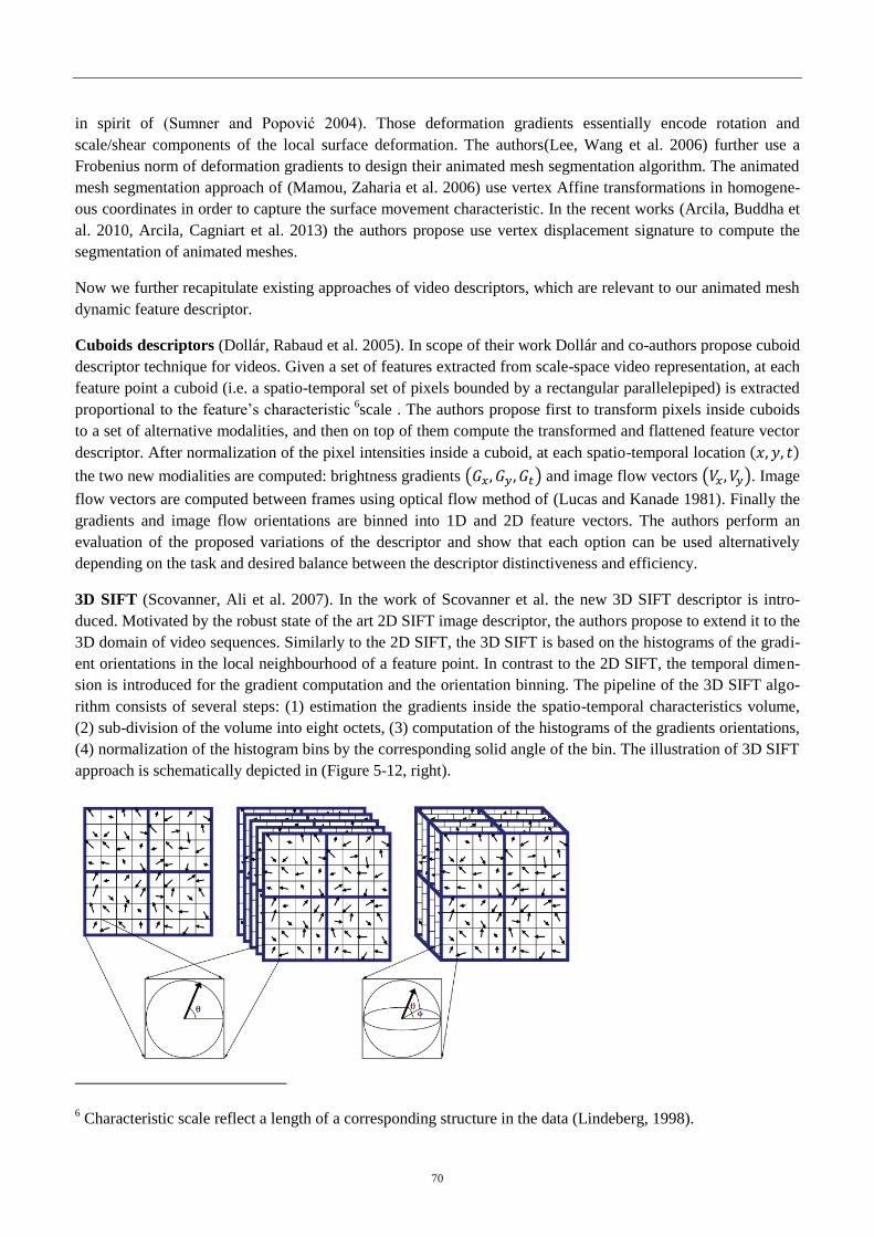
70

in spirit of (Sumner and Popović 2004). Those deformation gradients essentially encode rotation and

scale/shear components of the local surface deformation. The authors(Lee, Wang et al. 2006) further use a

Frobenius norm of deformation gradients to design their animated mesh segmentation algorithm. The animated

mesh segmentation approach of (Mamou, Zaharia et al. 2006) use vertex Affine transformations in homogene-

ous coordinates in order to capture the surface movement characteristic. In the recent works (Arcila, Buddha et

al. 2010, Arcila, Cagniart et al. 2013) the authors propose use vertex displacement signature to compute the

segmentation of animated meshes.

Now we further recapitulate existing approaches of video descriptors, which are relevant to our animated mesh

dynamic feature descriptor.

Cuboids descriptors (Dollár, Rabaud et al. 2005). In scope of their work Dollár and co-authors propose cuboid

descriptor technique for videos. Given a set of features extracted from scale-space video representation, at each

feature point a cuboid (i.e. a spatio-temporal set of pixels bounded by a rectangular parallelepiped) is extracted

proportional to the feature’s characteristic 6scale . The authors propose first to transform pixels inside cuboids

to a set of alternative modalities, and then on top of them compute the transformed and flattened feature vector

descriptor. After normalization of the pixel intensities inside a cuboid, at each spatio-temporal location

the two new modialities are computed: brightness gradients and image flow vectors . Image

flow vectors are computed between frames using optical flow method of (Lucas and Kanade 1981). Finally the

gradients and image flow orientations are binned into 1D and 2D feature vectors. The authors perform an

evaluation of the proposed variations of the descriptor and show that each option can be used alternatively

depending on the task and desired balance between the descriptor distinctiveness and efficiency.

3D SIFT (Scovanner, Ali et al. 2007). In the work of Scovanner et al. the new 3D SIFT descriptor is intro-

duced. Motivated by the robust state of the art 2D SIFT image descriptor, the authors propose to extend it to the

3D domain of video sequences. Similarly to the 2D SIFT, the 3D SIFT is based on the histograms of the gradi-

ent orientations in the local neighbourhood of a feature point. In contrast to the 2D SIFT, the temporal dimen-

sion is introduced for the gradient computation and the orientation binning. The pipeline of the 3D SIFT algo-

rithm consists of several steps: (1) estimation the gradients inside the spatio-temporal characteristics volume,

(2) sub-division of the volume into eight octets, (3) computation of the histograms of the gradients orientations,

(4) normalization of the histogram bins by the corresponding solid angle of the bin. The illustration of 3D SIFT

approach is schematically depicted in (Figure 5-12, right).

6 Characteristic scale reflect a length of a corresponding structure in the data (Lindeberg, 1998).

71

Figure 5-12. Classical 2D SIFT (left). Straightforward extension to the spatio-temporal domain without modification of the orig-

inal 2D SIFT (middle). 3D SIFT approach with the gradients computed over spatio-temporal volume (Scovanner, Ali et al.

2007).

HOG3D (Klaser and Marszalek 2008). Histogram of Oriented Gradients (HOG) (Dalal and Triggs 2005) are

feature descriptors used in computer vision and image processing for the purpose of object detection. The tech-

nique counts occurrences of gradient orientation in localized portions of an image. This method is similar to

scale-invariant feature transform (Scovanner, Ali et al. 2007) descriptors, and shape contexts (Körtgen, Park et

al. 2003), but differs in that it is computed on a dense grid of uniformly spaced cells and uses overlapping local

contrast normalization for improved accuracy. (Klaser and Marszalek 2008) propose a new descriptor for video

sequences based on orientations of spatio-temporal 3D gradients. First, the spatio-temporal gradients are effi-

ciently computed in the volume of interest in the video. Extending analogy from 2D, where n-bin histogram can

be seen as an approximation of a circle, the authors quantize the 3D gradient histogram in regular n-sided poly-

hedron. Then the HOG3D descriptor is computed by pooling the spatio-temporal gradient orientations in 3D

histogram over the polyhedron (Figure 5-13).

Figure 5-13. The computation pipeline of the HOG3D descriptor (Klaser and Marszalek 2008).

HoG/HoF. HoF desrciptor stands for Histogram of Oriented Optical Flow and also know in the literature as

Internal Motion Histograms (Dalal, Triggs et al. 2006, Laptev, Marszalek et al. 2008). Dalal et al. (Dalal,

Triggs et al. 2006) apply HoG/HoF detectors/descriptors to the problem of human detection in films and videos.

Essentially the proposed technique involves the combination of regular HOG descriptors on individual video

frames with the new HoF(IMH) descriptors on pairs of subsequent video frames. The Internal Motion Histo-

grams (IMH) uses the gradient magnitudes from optical flow fields obtained from two consecutive frames. The

gradient magnitudes of the optical flow are then used in the same manner as those produced from static image

data within the HoG descriptor approach.

Extended SURF (3D SURF). Willems et al. (Willems, Tuytelaars et al. 2008) introduce an extension of the

state-of-the-art Speed Up Robust Features (SURF) (Bay, Tuytelaars et al. 2006) image feature descriptor to the

3D domain. The SURF descriptor gained a reputation of a robust scale- and rotation-invariant feature detec-

tor/descriptor for images, therefore it is interesting to consider similar solution in more general spatio-temporal

video domain. In order to describe a point of interest with spatio-temporal characteristic scales, a rectangular

volume of dimensions proportional to characteristic scales is established around the feature point. Analogously

to the previous methods (Scovanner, Ali et al. 2007, Klaser and Marszalek 2008), the volume is furthermore

split into sub-volumes. The key idea of the proposed feature description is based on the classical SURF descrip-

tor (Bay, Tuytelaars et al. 2006). Extended SURF uses Wavelet responses in horizontal and vertical spatial di-

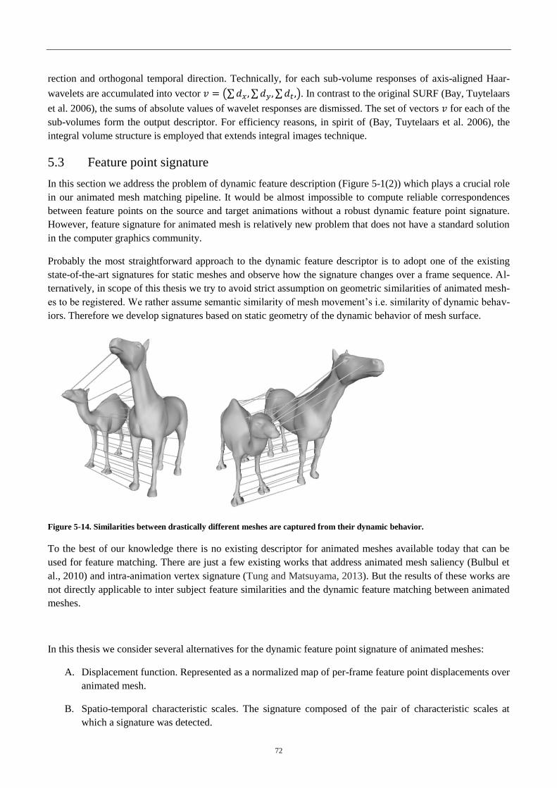
72

rection and orthogonal temporal direction. Technically, for each sub-volume responses of axis-aligned Haar-

wavelets are accumulated into vector . In contrast to the original SURF (Bay, Tuytelaars

et al. 2006), the sums of absolute values of wavelet responses are dismissed. The set of vectors for each of the

sub-volumes form the output descriptor. For efficiency reasons, in spirit of (Bay, Tuytelaars et al. 2006), the

integral volume structure is employed that extends integral images technique.

5.3 Feature point signature

In this section we address the problem of dynamic feature description (Figure 5-1(2)) which plays a crucial role

in our animated mesh matching pipeline. It would be almost impossible to compute reliable correspondences

between feature points on the source and target animations without a robust dynamic feature point signature.

However, feature signature for animated mesh is relatively new problem that does not have a standard solution

in the computer graphics community.

Probably the most straightforward approach to the dynamic feature descriptor is to adopt one of the existing

state-of-the-art signatures for static meshes and observe how the signature changes over a frame sequence. Al-

ternatively, in scope of this thesis we try to avoid strict assumption on geometric similarities of animated mesh-

es to be registered. We rather assume semantic similarity of mesh movement’s i.e. similarity of dynamic behav-

iors. Therefore we develop signatures based on static geometry of the dynamic behavior of mesh surface.

Figure 5-14. Similarities between drastically different meshes are captured from their dynamic behavior.

To the best of our knowledge there is no existing descriptor for animated meshes available today that can be

used for feature matching. There are just a few existing works that address animated mesh saliency (Bulbul et

al., 2010) and intra-animation vertex signature (Tung and Matsuyama, 2013). But the results of these works are

not directly applicable to inter subject feature similarities and the dynamic feature matching between animated

meshes.

In this thesis we consider several alternatives for the dynamic feature point signature of animated meshes:

A. Displacement function. Represented as a normalized map of per-frame feature point displacements over

animated mesh.

B. Spatio-temporal characteristic scales. The signature composed of the pair of characteristic scales at

which a signature was detected.

73

C. Histogram-of-Gradients for animated mesh

D. Deformation signature. The signature that captures deformation characteristics at a feature point over

frames in animation.

For each of the feature signature candidates we further develop the signature distance metric so that they can be

used for feature matching (5.5.1).

Hence we find it advantageous to largely exploit dynamic properties of animated meshes for the new feature

descriptor.

In the following sections we formally define each of these alternatives (sections 5.3.1-5.3.4). We evaluate their

time and storage complexities and formulate our final composite dynamic feature point signature in section

5.3.5.

5.3.1 Normalized displacement curves

In a recent work focusing on vertex saliency of animated meshes (Bulbul et al., 2010), Bulbul et al. present a

simple yet efficient method that identifies salient regions in animation meshes. The velocity saliency of a vertex

is calculated by taking the positional difference of a vertex in consecutive frames divided by the length of the

main diagonal of the mesh bounding box. Though Bulbul et al. refer as velocity to such saliency measure, one

can easily see that it is frame rate independent and therefore measures absolute displacements rather than veloc-

ity. Given a feature point from the extracted dynamic feature point set P, one can calculate the magnitude

of inter-frame displacement of a feature point p with respect to the previous frame in world coordinate system.

In Definition 3 we give a formal description of the displacement curve signature.

Definition 3. The displacement signature of a feature point p is defined as a function that maps

all the frames from animated mesh to the corresponding Euclidean displacement values

,

where is the global coordinate of the feature point p in the frame f and M is the number of frames in the

animation.

However displacement curve captures values of absolute vertex movement, which is not desirable for a

point signature. Typically, the displacement curve is directly proportional to the isotropic scale of animated

mesh (Figure 5-15).

We note that it is more advantageous to define the displacement curve that is invariant to the mesh scale. The

main function of the scale invariant signature is to compensate differences in absolute motion between source

and target meshes due to their scales i.e. absolute size. To this end we compare the relative movement of each

vertex between two consecutive frames by dividing by the global maximum displacement in the given ani-

mation . The normalized displacement curve signature that is invariant to absolute vertex movement defined

as

,

where .

(5-1)

In Figure 5-15 we plot of the displacement curve and normalized displacement curve signatures for the feature

point of the walking woman animation. In Figure 5-16 a comparison of normalized displacement curves is de-

picted for the corresponding features in the walking woman and walking baby animations.

74

(a) (b) (c)

Figure 5-15. Left: the displacement curve of the feature point on the right elbow of the walking woman (a). Displacement

curves corresponding to the feature point on the elbow of the original animated mesh and walking woman animation that was

isotropically enlarged by a scale factor of 2 (b). Normalized version of the displacement curve.

(a) (b)

(c) (d)

Figure 5-16. Normalized displacement curves for the walking woman and baby animations. Given consistently extracted feature

points on the wrist (a) and the knee (c), the corresponding normalized displacement curves are depicted in (b) and (d). Dis-

placement curves of the woman are shown in blue, while displacement curves of the baby are shown in cyan.

Distance metric. Given feature point from the source and feature point from the target, the distance be-

tween two normalized displacement curve signatures is defined as l2-norm of the difference between the two

curves:

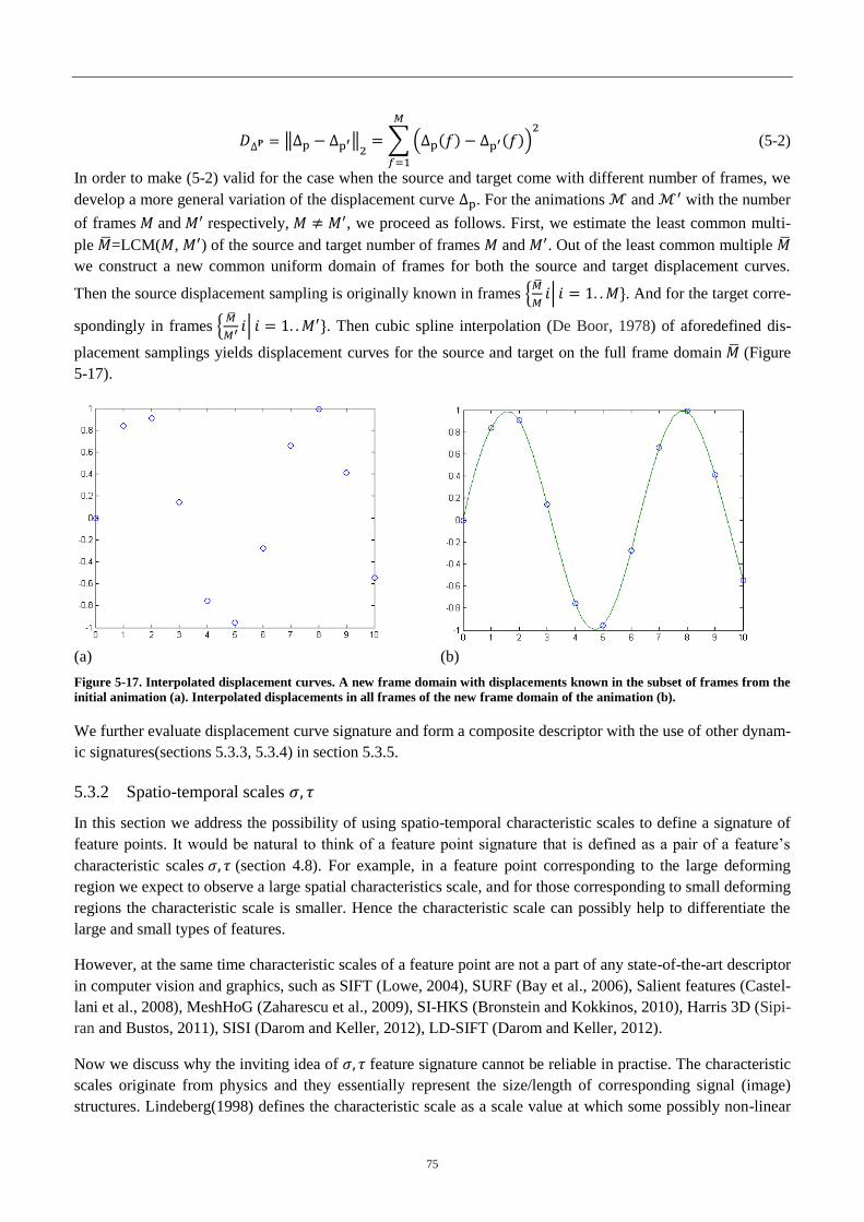
75

(5-2)

In order to make (5-2) valid for the case when the source and target come with different number of frames, we

develop a more general variation of the displacement curve . For the animations and with the number

of frames and respectively, , we proceed as follows. First, we estimate the least common multi-

ple =LCM( , ) of the source and target number of frames and . Out of the least common multiple

we construct a new common uniform domain of frames for both the source and target displacement curves.

Then the source displacement sampling is originally known in frames

. And for the target corre-

spondingly in frames

. Then cubic spline interpolation (De Boor, 1978) of aforedefined dis-

placement samplings yields displacement curves for the source and target on the full frame domain (Figure

5-17).

(a)

(b)

Figure 5-17. Interpolated displacement curves. A new frame domain with displacements known in the subset of frames from the

initial animation (a). Interpolated displacements in all frames of the new frame domain of the animation (b).

We further evaluate displacement curve signature and form a composite descriptor with the use of other dynam-

ic signatures(sections 5.3.3, 5.3.4) in section 5.3.5.

5.3.2 Spatio-temporal scales

In this section we address the possibility of using spatio-temporal characteristic scales to define a signature of

feature points. It would be natural to think of a feature point signature that is defined as a pair of a feature’s

characteristic scales (section 4.8). For example, in a feature point corresponding to the large deforming

region we expect to observe a large spatial characteristics scale, and for those corresponding to small deforming

regions the characteristic scale is smaller. Hence the characteristic scale can possibly help to differentiate the

large and small types of features.

However, at the same time characteristic scales of a feature point are not a part of any state-of-the-art descriptor

in computer vision and graphics, such as SIFT (Lowe, 2004), SURF (Bay et al., 2006), Salient features (Castel-

lani et al., 2008), MeshHoG (Zaharescu et al., 2009), SI-HKS (Bronstein and Kokkinos, 2010), Harris 3D (Sipi-

ran and Bustos, 2011), SISI (Darom and Keller, 2012), LD-SIFT (Darom and Keller, 2012).

Now we discuss why the inviting idea of feature signature cannot be reliable in practise. The characteristic

scales originate from physics and they essentially represent the size/length of corresponding signal (image)

structures. Lindeberg(1998) defines the characteristic scale as a scale value at which some possibly non-linear

76

combination of normalized derivatives assumes a local maximum over multi-scale representation of input data.

This definition induces the following properties:

1. The scale value at which a scale-normalized feature response operator reaches extremum is inversely

proportional to square of input signal frequency. It implies that given scaled structures in the input data,

the feature points are identified at coarser (larger) scales.

2. Presence of unique structure of given characteristic scales within a signal cannot be guaranteed. In par-

ticular, for the case of animated mesh, it is possible that different feature points (i.e. in different spatio

temporal locations) are extracted at similar characteristic scales. This is illustrated in (Figure 5-19).

Similarly, semantically identical feature points can be extracted at different characteristic scales.

In Figure 5-18, we make a plain illustration of the property (1). For simplicity we can consider a sinusoidal

input signal in one dimension, , of a frequency . Consider a scale space of the signal

, where s denotes a Gaussian kernel width. As Lindeberg (1998) shows, the maximum value

of the mth order scale-normalized derivative response operator over is independent of the

frequency . However, the argument of the maximum . is inversely proportional to

the square of the frequency (Figure 5-18).

Figure 5-18. The amplitude of first order normalized derivatives as function of scale for sinusoidal input signals of different

fr q cy ω1 = 0.5, ω2 = 1.0 ω3 = 2.0) (Lindeberg, 1998). Although is independent of the signal frequency ,

the scale argument of the maximum inversely proportional to the square the signal frequency .

(a) Frame 7, (b) Frame 29, (c) Frame 38,

Figure 5-19. Semantically different feature points are extracted at similar characteristic scales at different spatial and temporal

locations (a-c). In such a case the characteristic scales cannot help to differentiate between given feature points. The characteris-

tic scales represent the size of the deforming shape areas rather than the way the shapes actually deforms.

In our case of deformation characteristics signal originating from the animated mesh, properties (1-2) of charac-

teristic scales have the following direct consequences:

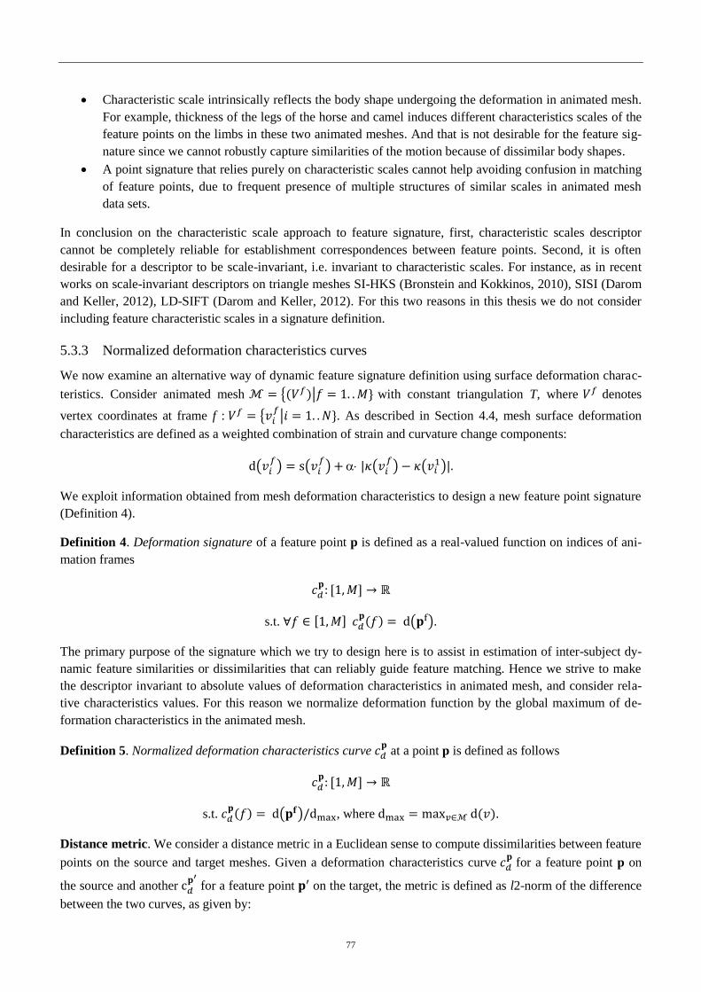
77

Characteristic scale intrinsically reflects the body shape undergoing the deformation in animated mesh.

For example, thickness of the legs of the horse and camel induces different characteristics scales of the

feature points on the limbs in these two animated meshes. And that is not desirable for the feature sig-

nature since we cannot robustly capture similarities of the motion because of dissimilar body shapes.

A point signature that relies purely on characteristic scales cannot help avoiding confusion in matching

of feature points, due to frequent presence of multiple structures of similar scales in animated mesh

data sets.

In conclusion on the characteristic scale approach to feature signature, first, characteristic scales descriptor

cannot be completely reliable for establishment correspondences between feature points. Second, it is often

desirable for a descriptor to be scale-invariant, i.e. invariant to characteristic scales. For instance, as in recent

works on scale-invariant descriptors on triangle meshes SI-HKS (Bronstein and Kokkinos, 2010), SISI (Darom

and Keller, 2012), LD-SIFT (Darom and Keller, 2012). For this two reasons in this thesis we do not consider

including feature characteristic scales in a signature definition.

5.3.3 Normalized deformation characteristics curves

We now examine an alternative way of dynamic feature signature definition using surface deformation charac-

teristics. Consider animated mesh with constant triangulation T, where denotes

vertex coordinates at frame f : . As described in Section 4.4, mesh surface deformation

characteristics are defined as a weighted combination of strain and curvature change components:

We exploit information obtained from mesh deformation characteristics to design a new feature point signature

(Definition 4).

Definition 4. Deformation signature of a feature point p is defined as a real-valued function on indices of ani-

mation frames

s.t. .

The primary purpose of the signature which we try to design here is to assist in estimation of inter-subject dy-

namic feature similarities or dissimilarities that can reliably guide feature matching. Hence we strive to make

the descriptor invariant to absolute values of deformation characteristics in animated mesh, and consider rela-

tive characteristics values. For this reason we normalize deformation function by the global maximum of de-

formation characteristics in the animated mesh.

Definition 5. Normalized deformation characteristics curve at a point p is defined as follows

s.t. , where .

Distance metric. We consider a distance metric in a Euclidean sense to compute dissimilarities between feature

points on the source and target meshes. Given a deformation characteristics curve for a feature point p on

the source and another

for a feature point on the target, the metric is defined as l2-norm of the difference

between the two curves, as given by:

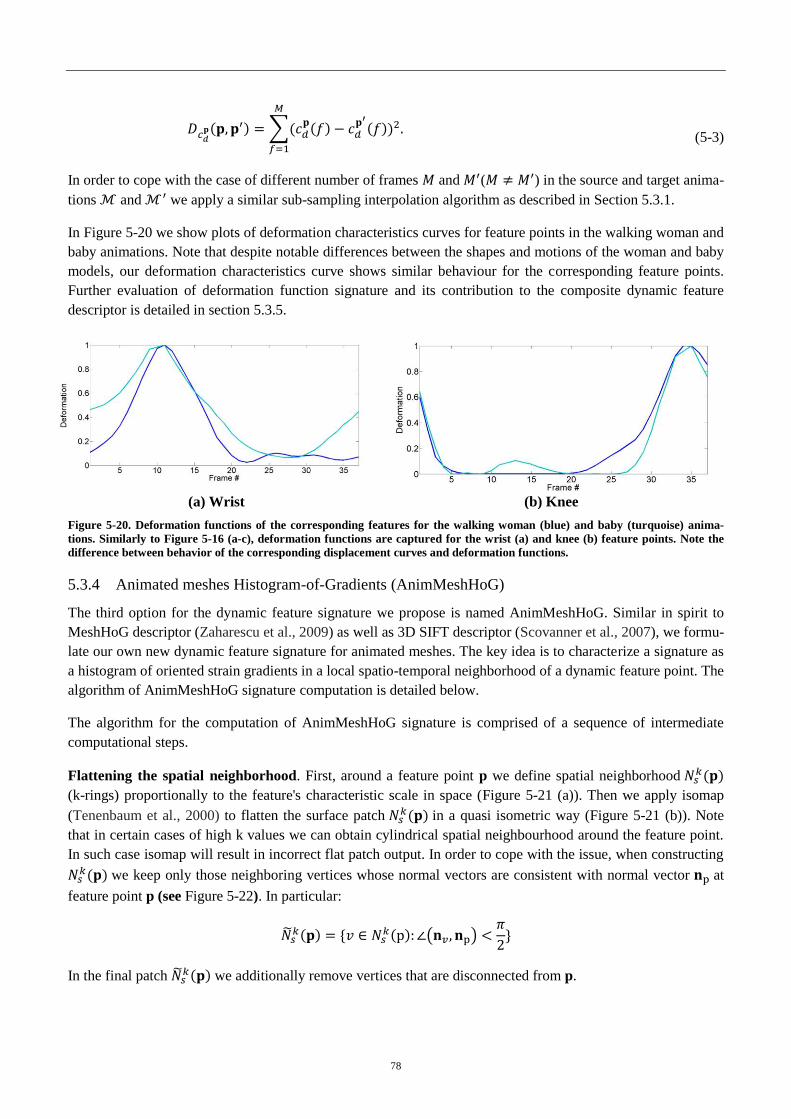
78

(5-3)

In order to cope with the case of different number of frames and ( ) in the source and target anima-

tions and we apply a similar sub-sampling interpolation algorithm as described in Section 5.3.1.

In Figure 5-20 we show plots of deformation characteristics curves for feature points in the walking woman and

baby animations. Note that despite notable differences between the shapes and motions of the woman and baby

models, our deformation characteristics curve shows similar behaviour for the corresponding feature points.

Further evaluation of deformation function signature and its contribution to the composite dynamic feature

descriptor is detailed in section 5.3.5.

(a) Wrist (b) Knee

Figure 5-20. Deformation functions of the corresponding features for the walking woman (blue) and baby (turquoise) anima-

tions. Similarly to Figure 5-16 (a-c), deformation functions are captured for the wrist (a) and knee (b) feature points. Note the

difference between behavior of the corresponding displacement curves and deformation functions.

5.3.4 Animated meshes Histogram-of-Gradients (AnimMeshHoG)

The third option for the dynamic feature signature we propose is named AnimMeshHoG. Similar in spirit to

MeshHoG descriptor (Zaharescu et al., 2009) as well as 3D SIFT descriptor (Scovanner et al., 2007), we formu-

late our own new dynamic feature signature for animated meshes. The key idea is to characterize a signature as

a histogram of oriented strain gradients in a local spatio-temporal neighborhood of a dynamic feature point. The

algorithm of AnimMeshHoG signature computation is detailed below.

The algorithm for the computation of AnimMeshHoG signature is comprised of a sequence of intermediate

computational steps.

Flattening the spatial neighborhood. First, around a feature point p we define spatial neighborhood

(k-rings) proportionally to the feature's characteristic scale in space (Figure 5-21 (a)). Then we apply isomap

(Tenenbaum et al., 2000) to flatten the surface patch in a quasi isometric way (Figure 5-21 (b)). Note

that in certain cases of high k values we can obtain cylindrical spatial neighbourhood around the feature point.

In such case isomap will result in incorrect flat patch output. In order to cope with the issue, when constructing

we keep only those neighboring vertices whose normal vectors are consistent with normal vector at

feature point p (see Figure 5-22). In particular:

In the final patch we additionally remove vertices that are disconnected from p.

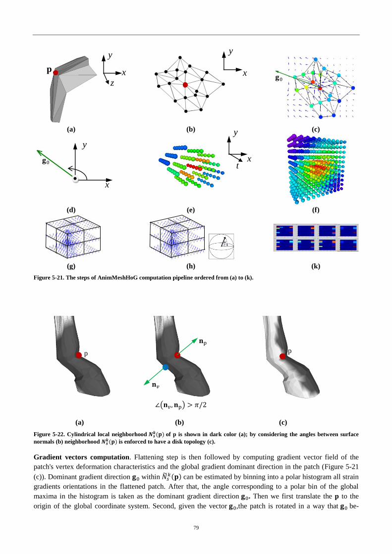
79

(a) (b) (c)

(d) (e) (f)

(g) (h) (k)

Figure 5-21. The steps of AnimMeshHoG computation pipeline ordered from (a) to (k).

(a) (b) (c)

Figure 5-22. Cylindrical local neighborhood of p is shown in dark color (a); by considering the angles between surface

normals (b) neighborhood is enforced to have a disk topology (c).

Gradient vectors computation. Flattening step is then followed by computing gradient vector field of the

patch's vertex deformation characteristics and the global gradient dominant direction in the patch (Figure 5-21

(c)). Dominant gradient direction within can be estimated by binning into a polar histogram all strain

gradients orientations in the flattened patch. After that, the angle corresponding to a polar bin of the global

maxima in the histogram is taken as the dominant gradient direction . Then we first translate the p to the

origin of the global coordinate system. Second, given the vector ,the patch is rotated in a way that be-

p p

x

y

y

x

y

x z

y

x t

p

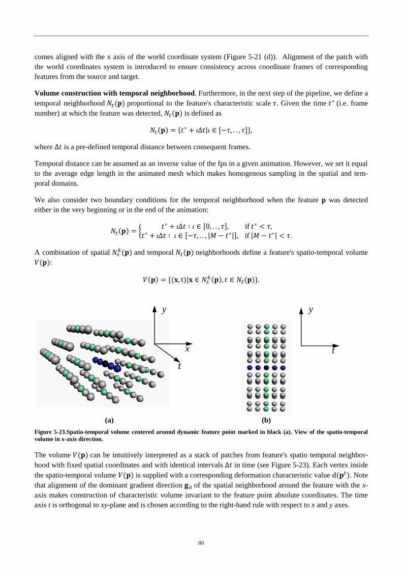
80

comes aligned with the x axis of the world coordinate system (Figure 5-21 (d)). Alignment of the patch with

the world coordinates system is introduced to ensure consistency across coordinate frames of corresponding

features from the source and target.

Volume construction with temporal neighborhood. Furthermore, in the next step of the pipeline, we define a

temporal neighborhood proportional to the feature's characteristic scale . Given the time (i.e. frame

number) at which the feature was detected, is defined as

,

where is a pre-defined temporal distance between consequent frames.

Temporal distance can be assumed as an inverse value of the fps in a given animation. However, we set it equal

to the average edge length in the animated mesh which makes homogenous sampling in the spatial and tem-

poral domains.

We also consider two boundary conditions for the temporal neighborhood when the feature p was detected

either in the very beginning or in the end of the animation:

A combination of spatial and temporal neighborhoods define a feature's spatio-temporal volume

:

.

(a) (b)

Figure 5-23.Spatio-temporal volume centered around dynamic feature point marked in black (a). View of the spatio-temporal

volume in x-axis direction.

The volume can be intuitively interpreted as a stack of patches from feature's spatio temporal neighbor-

hood with fixed spatial coordinates and with identical intervals in time (see Figure 5-23). Each vertex inside

the spatio-temporal volume is supplied with a corresponding deformation characteristic value . Note

that alignment of the dominant gradient direction of the spatial neighborhood around the feature with the x-

axis makes construction of characteristic volume invariant to the feature point absolute coordinates. The time

axis t is orthogonal to xy-plane and is chosen according to the right-hand rule with respect to x and y axes.

t

x t

y y

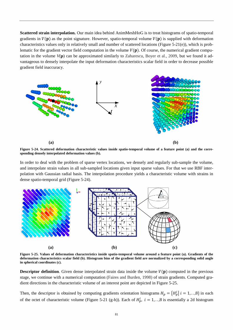
81

Scattered strain interpolation. Our main idea behind AnimMeshHoG is to treat histograms of spatio-temporal

gradients in as the point signature. However, spatio-temporal volume is supplied with deformation

characteristics values only in relatively small and number of scattered locations (Figure 5-21(e)), which is prob-

lematic for the gradient vector field computation in the volume . Of course, the numerical gradient compu-

tation in the volume V(p) can be approximated similarly to Zaharescu, Boyer et al., 2009, but we found it ad-

vantageous to densely interpolate the input deformation characteristics scalar field in order to decrease possible

gradient field inaccuracy.

(a) (b)

Figure 5-24. Scattered deformation characteristic values inside spatio-temporal volume of a feature point (a) and the corre-

sponding densely interpolated deformation values (b).

In order to deal with the problem of sparse vertex locations, we densely and regularly sub-sample the volume,

and interpolate strain values in all sub-sampled locations given input sparse values. For that we use RBF inter-

polation with Gaussian radial basis. The interpolation procedure yields a characteristic volume with strains in

dense spatio-temporal grid (Figure 5-24).

(a) (b) (c)

Figure 5-25. Values of deformation characteristics inside spatio-temporal volume around a feature point (a). Gradients of the

deformation characteristics scalar field (b). Histogram bins of the gradient field are normalized by a corresponding solid angle

in spherical coordinates (c).

Descriptor definition. Given dense interpolated strain data inside the volume computed in the previous

stage, we continue with a numerical computation (Faires and Burden, 1998) of strain gradients. Computed gra-

dient directions in the characteristic volume of an interest point are depicted in Figure 5-25.

Then, the descriptor is obtained by computing gradients orientation histograms in each

of the octet of characteristic volume (Figure 5-21 (g-h)). Each of is essentially a 2d histogram

t x

y

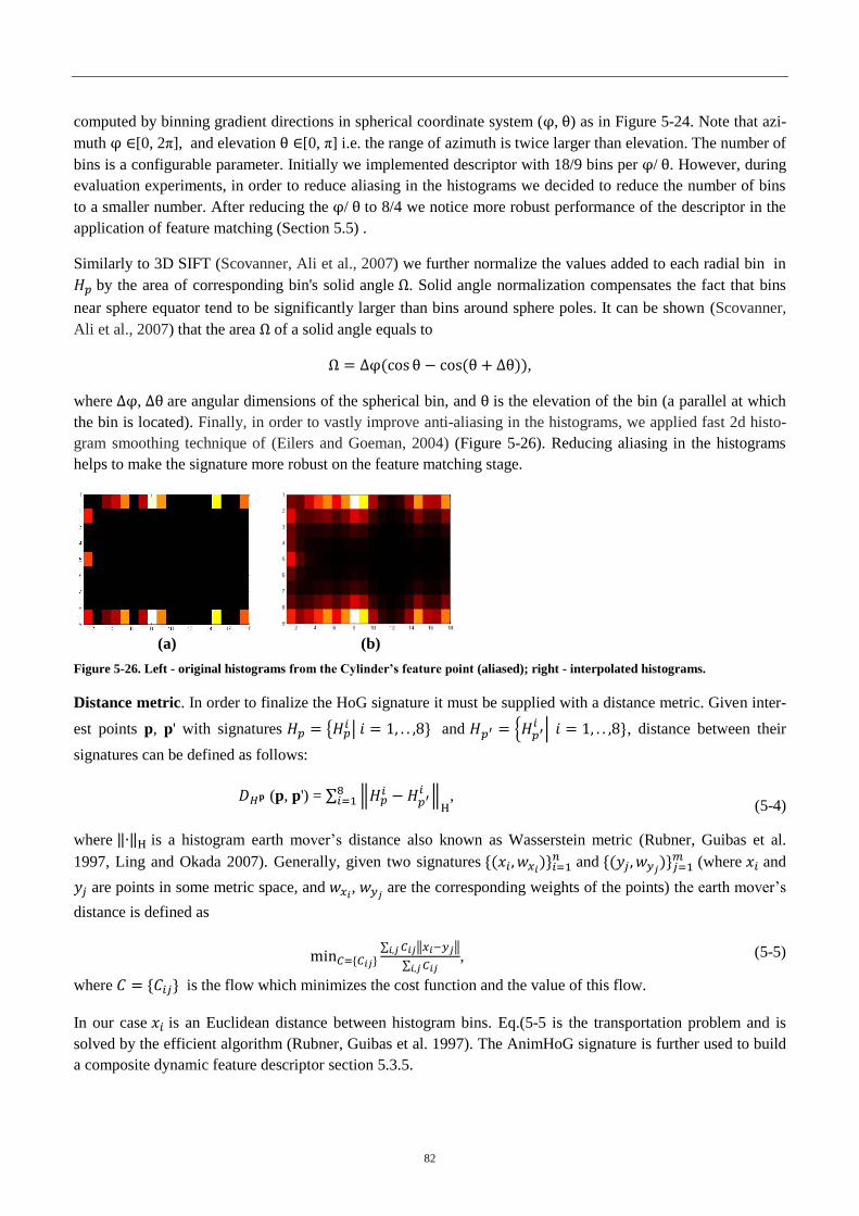
82

computed by binning gradient directions in spherical coordinate system ( , ) as in Figure 5-24. Note that azi-

muth [0, 2 ], and elevation [0, ] i.e. the range of azimuth is twice larger than elevation. The number of

bins is a configurable parameter. Initially we implemented descriptor with 18/9 bins per / . However, during

evaluation experiments, in order to reduce aliasing in the histograms we decided to reduce the number of bins

to a smaller number. After reducing the / to 8/4 we notice more robust performance of the descriptor in the

application of feature matching (Section 5.5) .

Similarly to 3D SIFT (Scovanner, Ali et al., 2007) we further normalize the values added to each radial bin in

by the area of corresponding bin's solid angle . Solid angle normalization compensates the fact that bins

near sphere equator tend to be significantly larger than bins around sphere poles. It can be shown (Scovanner,

Ali et al., 2007) that the area of a solid angle equals to

,

where , are angular dimensions of the spherical bin, and is the elevation of the bin (a parallel at which

the bin is located). Finally, in order to vastly improve anti-aliasing in the histograms, we applied fast 2d histo-

gram smoothing technique of (Eilers and Goeman, 2004) (Figure 5-26). Reducing aliasing in the histograms

helps to make the signature more robust on the feature matching stage.

(a) (b)

Figure 5-26. Left - original histograms fr t Cy r’s f t r p t (aliased); right - interpolated histograms.

Distance metric. In order to finalize the HoG signature it must be supplied with a distance metric. Given inter-

est points p, p' with signatures and

, distance between their

signatures can be defined as follows:

(p, p') =

,

(5-4)

where is a histogram earth mover’s distance also known as Wasserstein metric (Rubner, Guibas et al.

1997, Ling and Okada 2007). Generally, given two signatures and

(where and

are points in some metric space, and , are the corresponding weights of the points) the earth mover’s

distance is defined as

, (5-5)

where is the flow which minimizes the cost function and the value of this flow.

In our case is an Euclidean distance between histogram bins. Eq.(5-5 is the transportation problem and is

solved by the efficient algorithm (Rubner, Guibas et al. 1997). The AnimHoG signature is further used to build

a composite dynamic feature descriptor section 5.3.5.

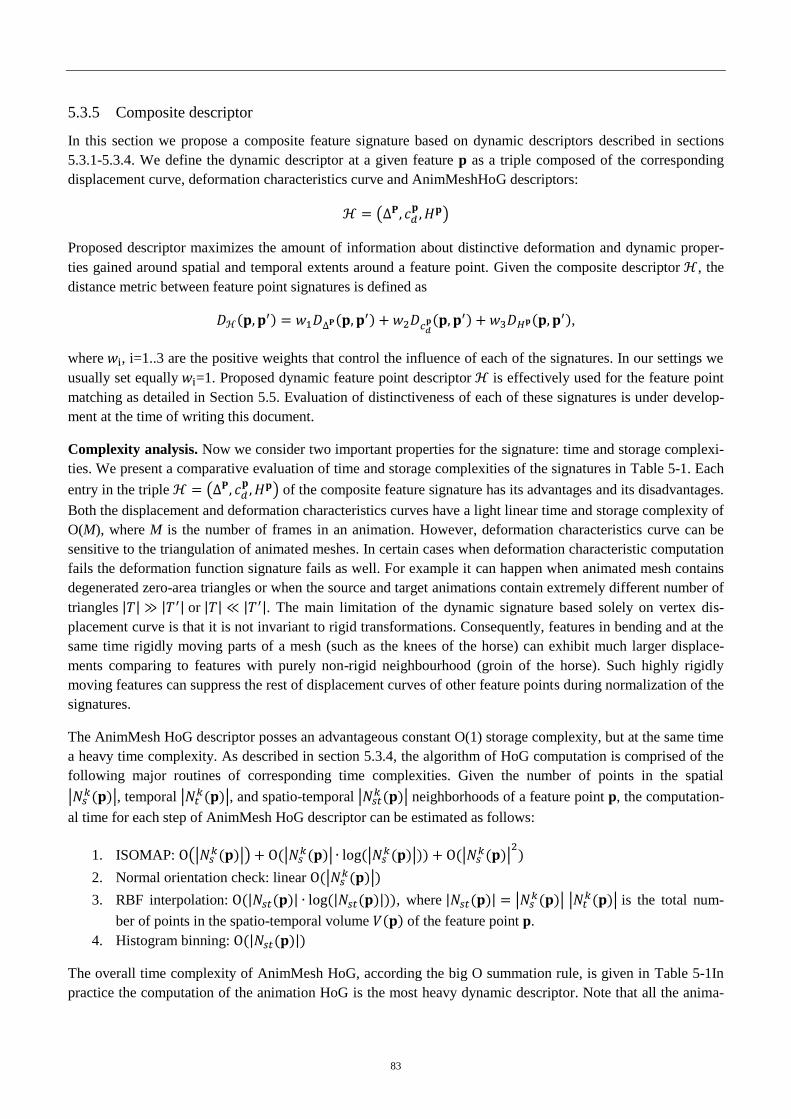
83

5.3.5 Composite descriptor

In this section we propose a composite feature signature based on dynamic descriptors described in sections

5.3.1-5.3.4. We define the dynamic descriptor at a given feature p as a triple composed of the corresponding

displacement curve, deformation characteristics curve and AnimMeshHoG descriptors:

Proposed descriptor maximizes the amount of information about distinctive deformation and dynamic proper-

ties gained around spatial and temporal extents around a feature point. Given the composite descriptor , the

distance metric between feature point signatures is defined as

,

where , i=1..3 are the positive weights that control the influence of each of the signatures. In our settings we

usually set equally =1. Proposed dynamic feature point descriptor is effectively used for the feature point

matching as detailed in Section 5.5. Evaluation of distinctiveness of each of these signatures is under develop-

ment at the time of writing this document.

Complexity analysis. Now we consider two important properties for the signature: time and storage complexi-

ties. We present a comparative evaluation of time and storage complexities of the signatures in Table 5-1. Each

entry in the triple of the composite feature signature has its advantages and its disadvantages.

Both the displacement and deformation characteristics curves have a light linear time and storage complexity of

O(M), where M is the number of frames in an animation. However, deformation characteristics curve can be

sensitive to the triangulation of animated meshes. In certain cases when deformation characteristic computation

fails the deformation function signature fails as well. For example it can happen when animated mesh contains

degenerated zero-area triangles or when the source and target animations contain extremely different number of

triangles or . The main limitation of the dynamic signature based solely on vertex dis-

placement curve is that it is not invariant to rigid transformations. Consequently, features in bending and at the

same time rigidly moving parts of a mesh (such as the knees of the horse) can exhibit much larger displace-

ments comparing to features with purely non-rigid neighbourhood (groin of the horse). Such highly rigidly

moving features can suppress the rest of displacement curves of other feature points during normalization of the

signatures.

The AnimMesh HoG descriptor posses an advantageous constant O(1) storage complexity, but at the same time

a heavy time complexity. As described in section 5.3.4, the algorithm of HoG computation is comprised of the

following major routines of corresponding time complexities. Given the number of points in the spatial

, temporal

, and spatio-temporal neighborhoods of a feature point p, the computation-

al time for each step of AnimMesh HoG descriptor can be estimated as follows:

1. ISOMAP:

2. Normal orientation check: linear

3. RBF interpolation: , where

is the total num-

ber of points in the spatio-temporal volume of the feature point p.

4. Histogram binning:

The overall time complexity of AnimMesh HoG, according the big O summation rule, is given in Table 5-1In

practice the computation of the animation HoG is the most heavy dynamic descriptor. Note that all the anima-

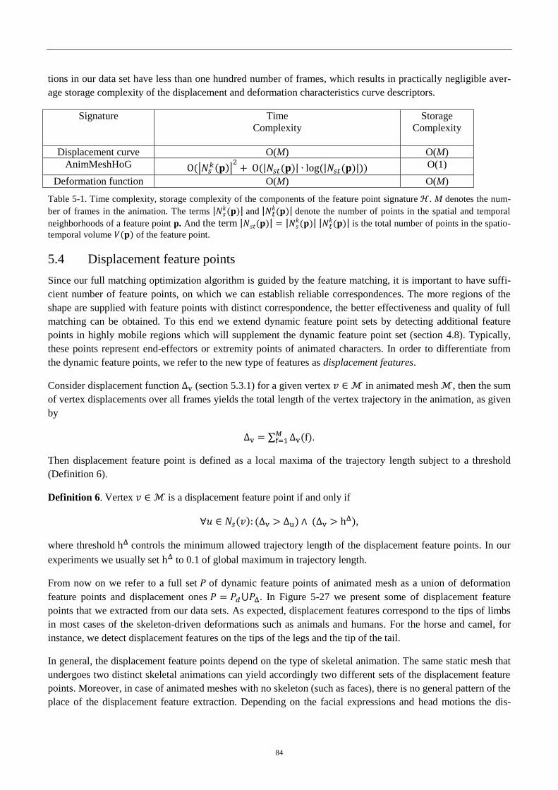
84

tions in our data set have less than one hundred number of frames, which results in practically negligible aver-

age storage complexity of the displacement and deformation characteristics curve descriptors.

Signature Time

Complexity

Storage

Complexity

Displacement curve O(M) O(M)

AnimMeshHoG

O(1)

Deformation function O(M) O(M)

Table 5-1. Time complexity, storage complexity of the components of the feature point signature . M denotes the num-

ber of frames in the animation. The terms and

denote the number of points in the spatial and temporal

neighborhoods of a feature point p. And the term

is the total number of points in the spatio-

temporal volume of the feature point.

5.4 Displacement feature points

Since our full matching optimization algorithm is guided by the feature matching, it is important to have suffi-

cient number of feature points, on which we can establish reliable correspondences. The more regions of the

shape are supplied with feature points with distinct correspondence, the better effectiveness and quality of full

matching can be obtained. To this end we extend dynamic feature point sets by detecting additional feature

points in highly mobile regions which will supplement the dynamic feature point set (section 4.8). Typically,

these points represent end-effectors or extremity points of animated characters. In order to differentiate from

the dynamic feature points, we refer to the new type of features as displacement features.

Consider displacement function (section 5.3.1) for a given vertex in animated mesh , then the sum

of vertex displacements over all frames yields the total length of the vertex trajectory in the animation, as given

by

.

Then displacement feature point is defined as a local maxima of the trajectory length subject to a threshold

(Definition 6).

Definition 6. Vertex is a displacement feature point if and only if

,

where threshold controls the minimum allowed trajectory length of the displacement feature points. In our

experiments we usually set to 0.1 of global maximum in trajectory length.

From now on we refer to a full set of dynamic feature points of animated mesh as a union of deformation

feature points and displacement ones . In Figure 5-27 we present some of displacement feature

points that we extracted from our data sets. As expected, displacement features correspond to the tips of limbs

in most cases of the skeleton-driven deformations such as animals and humans. For the horse and camel, for

instance, we detect displacement features on the tips of the legs and the tip of the tail.

In general, the displacement feature points depend on the type of skeletal animation. The same static mesh that

undergoes two distinct skeletal animations can yield accordingly two different sets of the displacement feature

points. Moreover, in case of animated meshes with no skeleton (such as faces), there is no general pattern of the

place of the displacement feature extraction. Depending on the facial expressions and head motions the dis-

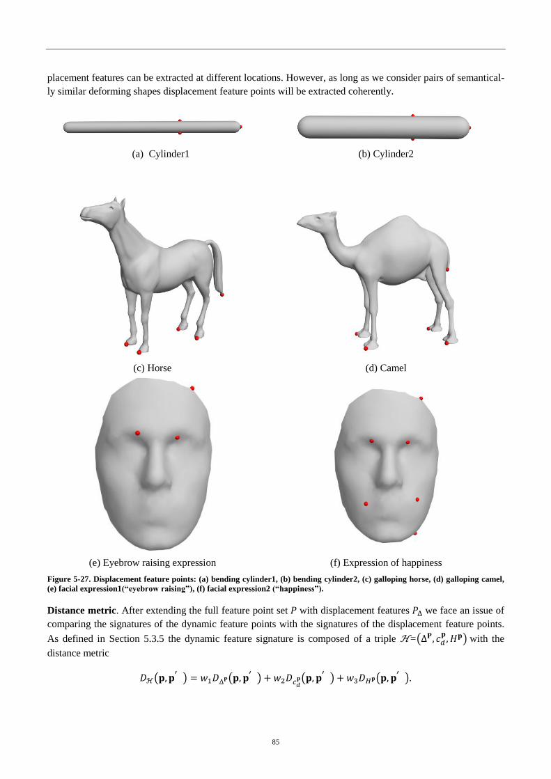
85

placement features can be extracted at different locations. However, as long as we consider pairs of semantical-

ly similar deforming shapes displacement feature points will be extracted coherently.

(a) Cylinder1

(b) Cylinder2

(c) Horse (d) Camel

(e) Eyebrow raising expression (f) Expression of happiness

Figure 5-27. Displacement feature points: (a) bending cylinder1, (b) bending cylinder2, (c) galloping horse, (d) galloping camel,

(e) facial expression1 “ y br w r s g”), (f) facial expression2 “ pp ss”).

Distance metric. After extending the full feature point set with displacement features we face an issue of

comparing the signatures of the dynamic feature points with the signatures of the displacement feature points.

As defined in Section 5.3.5 the dynamic feature signature is composed of a triple = with the

distance metric

.

86

Nevertheless it is important to note, that for obvious reasons, among all proposed dynamic feature signatures

we can rely only on displacement function for the measuring the similarity between displacement feature points

during matching. Moreover the same is true when comparing displacement to dynamic feature points. There-

fore we define the distance metric as

,

where p is a displacement feature and q is either displacement or dynamic feature point.

5.5 Feature correspondence via graph matching

Robust feature correspondence based on the dynamic feature point signature developed in section 5.3 is a first

and very important building block in the animated mesh matching pipeline (Figure 5-1). Naturally and similarly

to the majority of existing shape matching techniques, we cannot rely solely on the feature signatures to estab-

lish reliable correspondences between them. Therefore we take into account not only the signature of feature

points but also their relative spatial relationship. One of the most powerful mathematical tools that can provide

an accurate matching between two set of points based both on point signatures and relative spatial arrangement

is inexact graph isomorphism (inexact graph matching). Note, that in Chapter 6 we use a simpler Ullman’s

graph matching method for isometric shape correspondence, because the features involved in matching in

Chapter 6 are usually highly consistent. Here we propose to use the graph matching technique based on the

work of (Torresani, Kolmogorov et al., 2008, Torresani, Kolmogorov et al. 2013).

Unfortunately, inexact graph matching is a NP-hard problem (Gallagher, 2006). We have chosen to use the

graph matching via dual decomposition by (Torresani, Kolmogorov et al., 2008, Torresani, Kolmogorov et al.

2013) due to our several practical requirements for the feature matching technique:

1. Fast. The method should have a low computational complexity.

2. Inexact. We would like to adopt attributed subgraph matching which allows us to perform as best as

possible in matching between inconsistent feature point sets.

3. Robust. The method should produce stable and correct matching results in most of the cases. Even

though we assume similarities of the source and target animated meshes, their motions are not perfectly

the same in practice. This results in a faire amount of differences between the signatures of correspond-

ing features from the source and target animations in certain cases. Therefore graph matching algorithm

should allow to robustly handle variations of the point signatures of corresponding feature points.

In the work of(Torresani, Kolmogorov et al. 2013) the authors compare Dual Decomposition graph matching

optimization to other state-of-the-art graph matching techniques (Cour et al., 2007, Elidan et al., 2007,

Lempitsky et al., 2007) and demonstrate that their technique outperforms significantly existing graph matching

algorithms. We adopt a similar technique in our graph matching solution, however with important differences

that make it suitable for animated mesh dynamic feature matching. More specifically, we provide a way to the

graph matching algorithm to strongly penalize matches that are incompatible in geodesic sense on the source

and target meshes (Section 4.5.3).

5.5.1 Graph matching formulation

In this section, we show how we adapt the DD technique of (Torresani et al. 2008, Torresani, Kolmogorov et al.

2013) to our problem of feature matching for animated meshes. Given a set of feature points ,

={ , extracted from the source and target animations respectively, we propose to construct

feature graphs in the following way. First we discard the time coordinate by projecting the feature point sets on

87

the space domain: , ={ . Note, that we do not lose the temporal infor-

mation regarding a feature point since we compensate it in some of the feature point signatures (e.g. displace-

ment and deformation characteristics curves). It means that two features and detected at the same

spatial location p and different time are considered to be a same feature.

Then we define a set of possible assignments between feature points from the source and target.

The set represents potential matching pairs. Each assignment is supplied with a cost equal

to the distance (section 5.3.5) between corresponding feature descriptors. Instead of considering the

complete set of all possible assignments , each feature point is associated only with features

on the target that are closest in terms of feature signature. We further populate the set of assign-

ments by including matching pairs of features on target and features on the source with the most

similar signatures. The algorithm of assignment set construction is summarized in Algorithm 5-1. We typically

set to 4 throughout our experiments in this thesis.

Algorithm 5-1. The construction of assignment set. Input: Feature points sets on the source and target Output: Possible assignment set begin for each

(p) for each (

) end

Considering all feature point assignments to be the nodes of complete graph, we now can formulate our objec-

tive function to be minimized as a weighted sum of energy terms:

( , (5-6)

where x is a binary-valued vector representing a feature matching solution. Each value in x is

associated with an assignment a. If then the assignment a is included in feature matching solution (i.e.

assignment a is active), and it is not included if (a is inactive). energy term estimates nodes dis-

similarities (distance in section 5.3.5), describes edge dissimilarities and , are stabiliz-

ing terms enforcing valid graph matching results. We detail each of the energy terms below.

Descriptor energy term. Descriptor energy term measures similarities between feature point signatures in-

volved in active assignments

,

with defined as the distance (section 5.3.5) between feature points involved in assignment

. The term favours matching solutions of features with similar signatures (descriptors).

Geodesic distortion term. We further define an important geodesic distortion term that measures how

much the relative geodesic distance between feature points p, q on the source is preserved between their corre-

spondences , on the target.

Let be a set of neighbouring correspondence pairs (Torresani, Kolmogorov et al. 2008)

where is a set of k nearest neighbours of feature point p. For our matching experiments we used

constant k from interval [3,6].

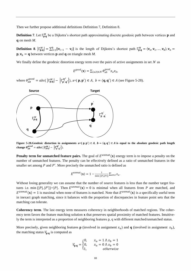
88

Then we further propose additional definitions Definition 7, Definition 8.

Definition 7. Let be a Dijkstra’s shortest path approximating discrete geodesic path between vertices and

on mesh M.

Definition 8.

is the length of Dijkstra’s shortest path

between vertices and on triangle mesh M.

We finally define the geodesic distortion energy term over the pairs of active assignments in set as

,

where

, a=( (see Figure 5-28).

,

q

p

,

Source Target

Figure 5-28.Geodesic distortion in assignments a=( is equal to the absolute geodesic path length

change

.

Penalty term for unmatched feature pairs. The goal of energy term is to impose a penalty on the

number of unmatched features. The penalty can be effectively defined as a ratio of unmatched features in the

smaller set among and . More precisely the unmatched ratio is defined as

.

Without losing generality we can assume that the number of source features is less than the number target fea-

tures i.e. = . Then is minimal when all features from P are matched, and

is maximal when none of features is matched. Note that is a specifically useful term

in inexact graph matching, since it balances with the proportion of discrepancies in feature point sets that the

matching can tolerate.

Coherency term. The last energy term measures coherency in neighborhoods of matched regions. The coher-

ency term favors the feature matching solution x that preserves spatial proximity of matched features. Intuitive-

ly the term is interpreted as a proportion of neighboring features p, q with different matched/unmatched status.

More precisely, given neighboring features p (involved in assignment ) and q (involved in assignment ),

the matching status is computed as

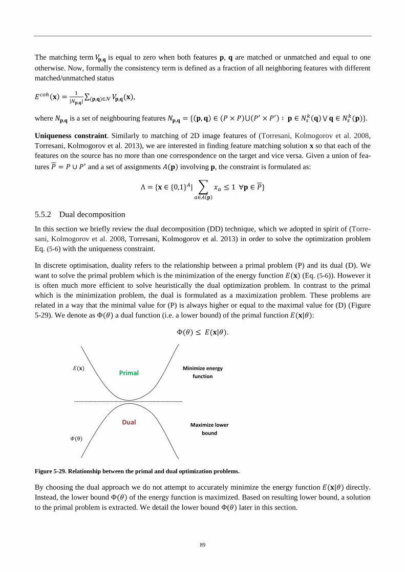
89

The matching term is equal to zero when both features p, q are matched or unmatched and equal to one

otherwise. Now, formally the consistency term is defined as a fraction of all neighboring features with different

matched/unmatched status

,

where is a set of neighbouring features

.

Uniqueness constraint. Similarly to matching of 2D image features of (Torresani, Kolmogorov et al. 2008,

Torresani, Kolmogorov et al. 2013), we are interested in finding feature matching solution x so that each of the

features on the source has no more than one correspondence on the target and vice versa. Given a union of fea-

tures and a set of assignments involving p, the constraint is formulated as:

5.5.2 Dual decomposition

In this section we briefly review the dual decomposition (DD) technique, which we adopted in spirit of (Torre-

sani, Kolmogorov et al. 2008, Torresani, Kolmogorov et al. 2013) in order to solve the optimization problem

Eq. (5-6) with the uniqueness constraint.

In discrete optimisation, duality refers to the relationship between a primal problem (P) and its dual (D). We

want to solve the primal problem which is the minimization of the energy function (Eq. (5-6)). However it

is often much more efficient to solve heuristically the dual optimization problem. In contrast to the primal

which is the minimization problem, the dual is formulated as a maximization problem. These problems are

related in a way that the minimal value for (P) is always higher or equal to the maximal value for (D) (Figure

5-29). We denote as a dual function (i.e. a lower bound) of the primal function :

.

Primal

Dual

𝛷( )

( ) Minimize energy

function

Maximize lower

bound

Figure 5-29. Relationship between the primal and dual optimization problems.

By choosing the dual approach we do not attempt to accurately minimize the energy function directly.

Instead, the lower bound of the energy function is maximized. Based on resulting lower bound, a solution

to the primal problem is extracted. We detail the lower bound ( later in this section.

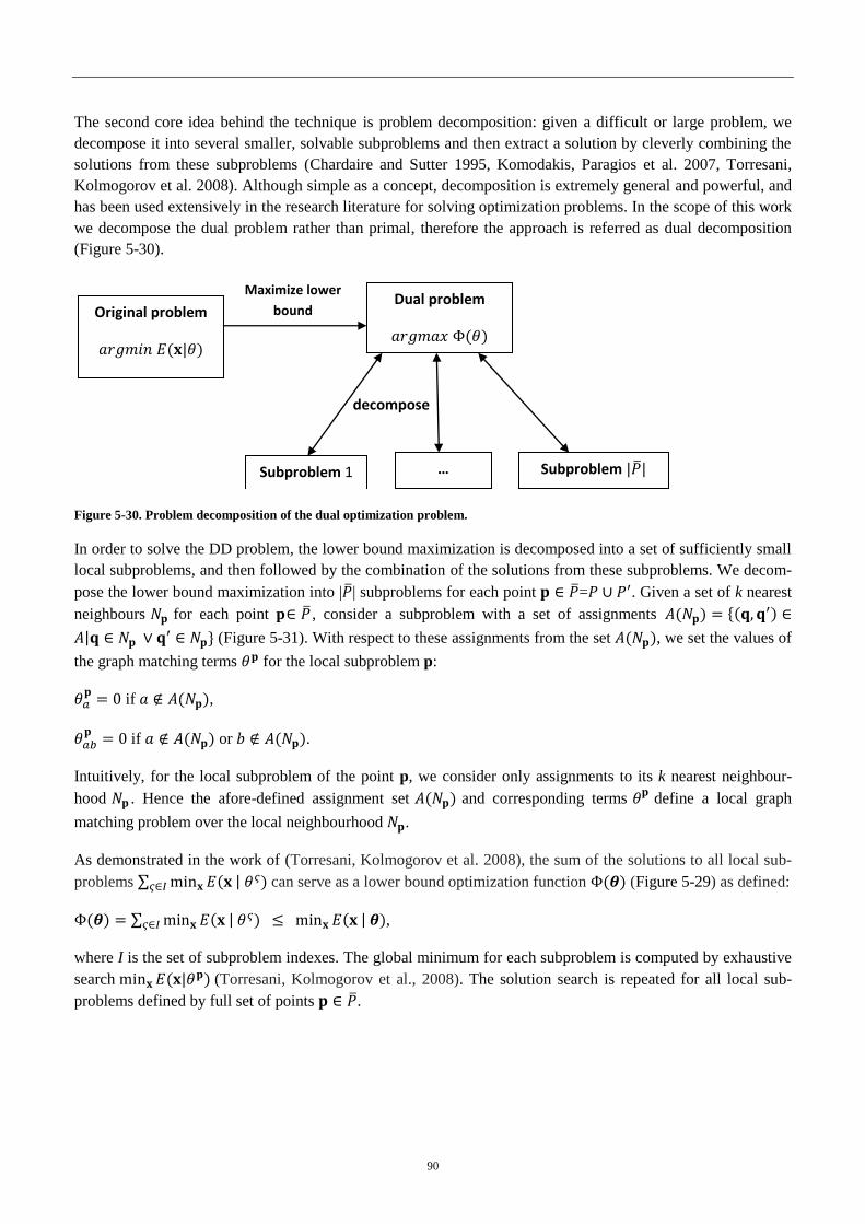
90

The second core idea behind the technique is problem decomposition: given a difficult or large problem, we

decompose it into several smaller, solvable subproblems and then extract a solution by cleverly combining the

solutions from these subproblems (Chardaire and Sutter 1995, Komodakis, Paragios et al. 2007, Torresani,

Kolmogorov et al. 2008). Although simple as a concept, decomposition is extremely general and powerful, and

has been used extensively in the research literature for solving optimization problems. In the scope of this work

we decompose the dual problem rather than primal, therefore the approach is referred as dual decomposition

(Figure 5-30).

( | )

Original problem

… Subproblem | | Subproblem 1

( )

Dual problem Maximize lower

bound

decompose

Figure 5-30. Problem decomposition of the dual optimization problem.

In order to solve the DD problem, the lower bound maximization is decomposed into a set of sufficiently small

local subproblems, and then followed by the combination of the solutions from these subproblems. We decom-

pose the lower bound maximization into | | subproblems for each point = . Given a set of k nearest

neighbours for each point p , consider a subproblem with a set of assignments

(Figure 5-31). With respect to these assignments from the set , we set the values of

the graph matching terms for the local subproblem p:

if ,

if or .

Intuitively, for the local subproblem of the point p, we consider only assignments to its k nearest neighbour-

hood . Hence the afore-defined assignment set and corresponding terms define a local graph

matching problem over the local neighbourhood .

As demonstrated in the work of (Torresani, Kolmogorov et al. 2008), the sum of the solutions to all local sub-

problems can serve as a lower bound optimization function (Figure 5-29) as defined:

,

where I is the set of subproblem indexes. The global minimum for each subproblem is computed by exhaustive

search (Torresani, Kolmogorov et al., 2008). The solution search is repeated for all local sub-

problems defined by full set of points .

91

Subproblem 2

Subproblem 1

Subproblem 3

P P’

p

Np

… …

Figure 5-31. Local subproblem decomposition. For each point p, local subproblem involves only assignments within the local

neighbourhood .

Then, given the solutions for all local subproblems, the lower bound is maxi-

mized via classical optimization subgradient method as presented in (Shor 1985, Chardaire and Sutter 1995,

Bertsekas 1999, Komodakis, Paragios et al. 2007, Schlesinger and Giginyak 2007, Torresani, Kolmogorov et

al. 2008). The subgradient maximization of recomputes subproblem solutions on each iteration until the

value of lower bound change between the next and previous iterations is less than a user threshold (Torresani,

Kolmogorov et al. 2008). Finally in order to obtain solution x we follow the technique of (Torresani, Kolmo-

gorov et al. 2008) so that at each iteration the solution is obtained in the way detailed in Algorithm 5-2.

Algorithm 5-2. Combining solutions of local subproblems into a global solution

Input: solutions , of all local subproblems

Output: output matching global solution x

begin

x=0

foreach subproblem

foreach assignment

if // if assignment is active in a subproblem

// then activate it the global solution

end

end

end

end

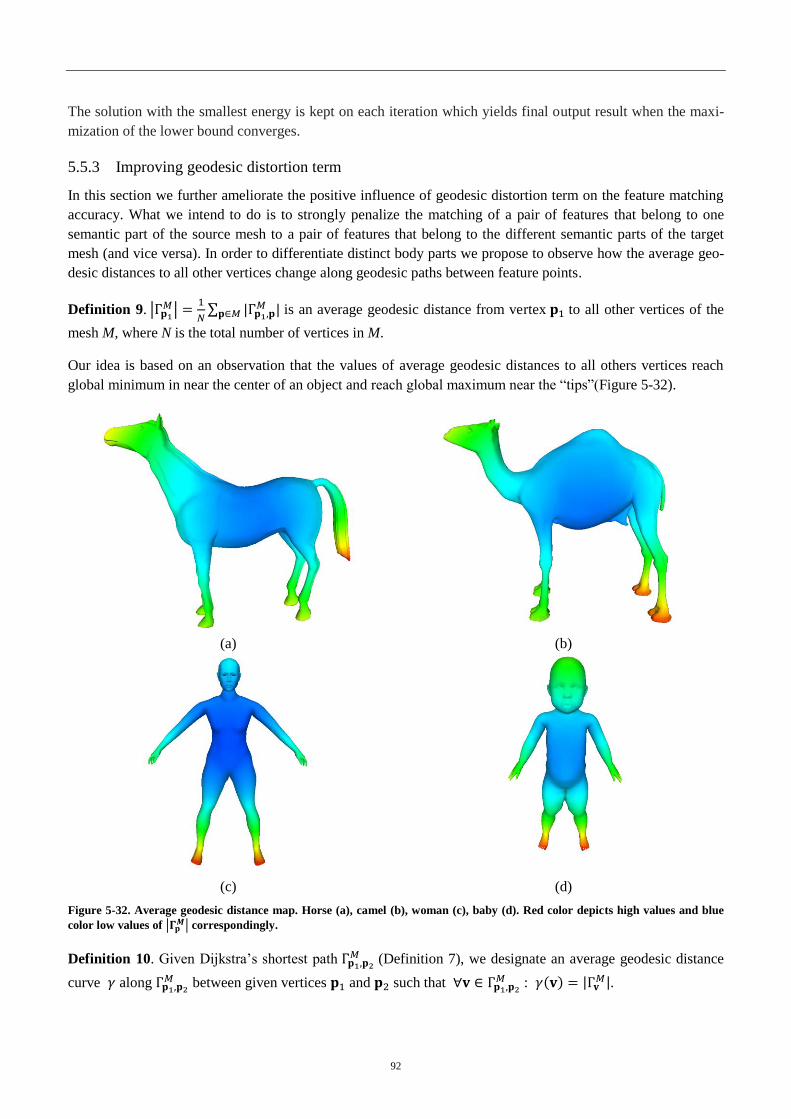
92

The solution with the smallest energy is kept on each iteration which yields final output result when the maxi-

mization of the lower bound converges.

5.5.3 Improving geodesic distortion term

In this section we further ameliorate the positive influence of geodesic distortion term on the feature matching

accuracy. What we intend to do is to strongly penalize the matching of a pair of features that belong to one

semantic part of the source mesh to a pair of features that belong to the different semantic parts of the target

mesh (and vice versa). In order to differentiate distinct body parts we propose to observe how the average geo-

desic distances to all other vertices change along geodesic paths between feature points.

Definition 9.

is an average geodesic distance from vertex to all other vertices of the

mesh M, where N is the total number of vertices in M.

Our idea is based on an observation that the values of average geodesic distances to all others vertices reach

global minimum in near the center of an object and reach global maximum near the “tips”(Figure 5-32).

(a) (b)

(c) (d)

Figure 5-32. Average geodesic distance map. Horse (a), camel (b), woman (c), baby (d). Red color depicts high values and blue

color low values of correspondingly.

Definition 10. Given Dijkstra’s shortest path (Definition 7), we designate an average geodesic distance

curve along between given vertices and such that

: .

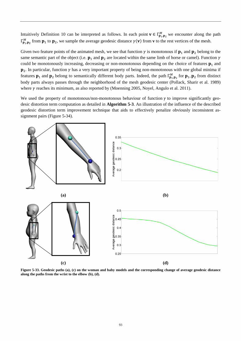
93

Intuitively Definition 10 can be interpreted as follows. In each point we encounter along the path

from to , we sample the average geodesic distance from v to the rest vertices of the mesh.

Given two feature points of the animated mesh, we see that function is monotonous if and belong to the

same semantic part of the object (i.e. and are located within the same limb of horse or camel). Function

could be monotonously increasing, decreasing or non-monotonous depending on the choice of features and

. In particular, function has a very important property of being non-monotonous with one global minima if

features and belong to semantically different body parts. Indeed, the path for from distinct

body parts always passes through the neighborhood of the mesh geodesic center (Pollack, Sharir et al. 1989)

where reaches its minimum, as also reported by (Moenning 2005, Noyel, Angulo et al. 2011).

We used the property of monotonous/non-monotonous behaviour of function to improve significantly geo-

desic distortion term computation as detailed in Algorithm 5-3. An illustration of the influence of the described

geodesic distortion term improvement technique that aids to effectively penalize obviously inconsistent as-

signment pairs (Figure 5-34).

(a)

(b)

(c) (d)

Figure 5-33. Geodesic paths (a), (c) on the woman and baby models and the corresponding change of average geodesic distance

along the paths from the wrist to the elbow (b), (d).

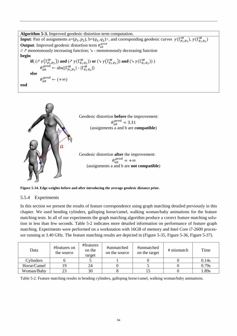
94

Algorithm 5-3. Improved geodesic distortion term computation.

Input: Pair of assignments a=( ), b=( )>, and corresponding geodesic curves ,

Output: Improved geodesic distortion term

// monotonously increasing function; - monotonously decreasing function

begin

if( ( ) and (

) or ( ) and (

) )

abs( -

)

else

end

Geodesic distortion before the improvement:

(assignments a and b are compatible)

Geodesic distortion after the improvement:

(assignments a and b are not compatible)

Figure 5-34. Edge weights before and after introducing the average geodesic distance prior.

5.5.4 Experiments

In this section we present the results of feature correspondence using graph matching detailed previously in this

chapter. We used bending cylinders, galloping horse/camel, walking woman/baby animations for the feature

matching tests. In all of our experiments the graph matching algorithm produce a correct feature matching solu-

tion in less than few seconds. Table 5-2 indicates more detailed information on performance of feature graph

matching. Experiments were performed on a workstation with 16GB of memory and Intel Core i7-2600 proces-

sor running at 3.40 GHz. The feature matching results are depicted in (Figure 5-35, Figure 5-36, Figure 5-37).

Data #features on

the source

#features

on the

target

#unmatched

on the source

#unmatched

on the target # mismatch Time

Cylinders 6 5 1 0 0 0.14s

Horse/Camel 19 24 0 5 0 0.79s

Woman/Baby 23 30 8 15 0 1.89s

Table 5-2. Feature matching results in bending cylinders, galloping horse/camel, walking woman/baby animations.

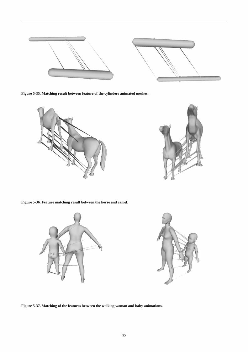
95

Figure 5-35. Matching result between feature of the cylinders animated meshes.

Figure 5-36. Feature matching result between the horse and camel.

Figure 5-37. Matching of the features between the walking woman and baby animations.

96

5.6 Full matching

5.6.1 Spherical embedding

Once we have computed the matching among feature vertices, we propagate the computed correspondence to

all points on the source mesh, which is the objective of the fine matching. The goal is to compute the one-to-

one correspondence (i.e. bijective mapping) between every point7 of the source mesh and that of the target

mesh with the feature constraint, i.e. the previously computed matching among the feature vertices is kept.

Methods combining the feature error, distortion (smoothness) error, and the data error could be adopted here

(Allen, Curless et al. 2003) (see Section 3.1). Due to the high dimensionality of the solution space (number of

vertices or sampled points multiplied by the degree of freedom, typically three), however, it is often unpractical

to search for the solution in such settings. In particular, measuring the data error term requires considerable

computation time, even with a data structure devoted to an efficient computation of the distance between the

two surfaces.

In this thesis, we propose to compute the bijective mapping in the spherical parameterization, the parameteriza-

tion of a genus-zero surface onto a spherical domain. Formally, the spherical parameterization of the mesh

is defined as:

, where .

Every point of the spherically parameterized mesh is located on the surface of a unit sphere centered at the

origin. With the meshes embedded in the unit sphere, the problem of surface matching in the 3D space is sim-

plified to that of matching in the 2D spherical domain. This not only reduces the dimensionality of the problem

but also removes the need for the heavy computation of the data error term. In addition, there exist several

methods (Saba, Yavneh et al. 2005, Praun and Hoppe 2003) to compute this parameterization efficiently.

Let and be the source and target meshes respectively; and are their spherical parameteri-

zation respectively. Also let be the bijective mapping of to and the bijective

mapping of to . Then a bijective mapping between the source and the target meshes can be obtained

by computing:

(see Figure 5-38)

The bijectivity of the composite function is guaranteed if each of the three functions involved is bijective. The

mappings and we obtain from the spherical parameterization, which are both bijective.

Thus we concentrate on the problem of finding that is bijective while satisfying the aforementioned

feature constraints.

7 Here, we distinguish an arbitrarily sampled point on the mesh surface from a vertex (point comprising the

mesh).

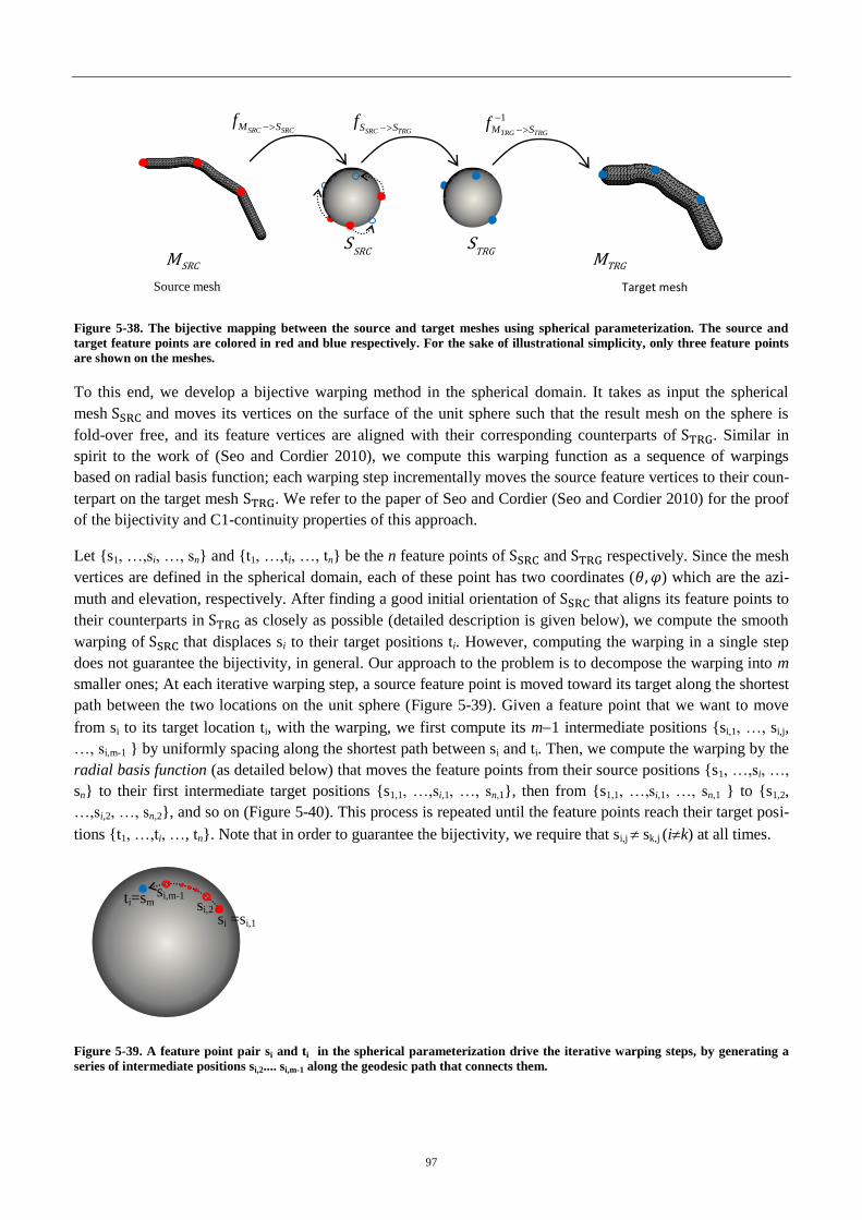
97

Figure 5-38. The bijective mapping between the source and target meshes using spherical parameterization. The source and

target feature points are colored in red and blue respectively. For the sake of illustrational simplicity, only three feature points

are shown on the meshes.

To this end, we develop a bijective warping method in the spherical domain. It takes as input the spherical

mesh and moves its vertices on the surface of the unit sphere such that the result mesh on the sphere is

fold-over free, and its feature vertices are aligned with their corresponding counterparts of . Similar in

spirit to the work of (Seo and Cordier 2010), we compute this warping function as a sequence of warpings

based on radial basis function; each warping step incrementally moves the source feature vertices to their coun-

terpart on the target mesh . We refer to the paper of Seo and Cordier (Seo and Cordier 2010) for the proof

of the bijectivity and C1-continuity properties of this approach.

Let {s1, …,si, …, sn} and {t1, …,ti, …, tn} be the n feature points of and respectively. Since the mesh

vertices are defined in the spherical domain, each of these point has two coordinates ( ) which are the azi-

muth and elevation, respectively. After finding a good initial orientation of that aligns its feature points to

their counterparts in as closely as possible (detailed description is given below), we compute the smooth

warping of that displaces si to their target positions ti. However, computing the warping in a single step

does not guarantee the bijectivity, in general. Our approach to the problem is to decompose the warping into m

smaller ones; At each iterative warping step, a source feature point is moved toward its target along the shortest

path between the two locations on the unit sphere (Figure 5-39). Given a feature point that we want to move

from si to its target location ti, with the warping, we first compute its m1 intermediate positions {si,1, …, si,j,

…, si,m-1 } by uniformly spacing along the shortest path between si and ti. Then, we compute the warping by the

radial basis function (as detailed below) that moves the feature points from their source positions {s1, …,si, …,

sn} to their first intermediate target positions {s1,1, …,si,1, …, sn,1}, then from {s1,1, …,si,1, …, sn,1 } to {s1,2,

…,si,2, …, sn,2}, and so on (Figure 5-40). This process is repeated until the feature points reach their target posi-

tions {t1, …,ti, …, tn}. Note that in order to guarantee the bijectivity, we require that si,j sk,j (ik) at all times.

Figure 5-39. A feature point pair si and ti in the spherical parameterization drive the iterative warping steps, by generating a

series of intermediate positions si,2.... si,m-1 along the geodesic path that connects them.

ti=sm si,2

si,m-1

Source mesh Target mesh

SRCMSRC

STRG

S

SRC SRCM Sf SRC TRGS Sf

TRGM

1

TRG TRGM Sf

si =si,1

98

(a) (b) (c) (d)

Figure 5-40. Warping of the mesh vertices to move the source feature points (shown in blue) to their target position (shown in

red). Figures (a) and (b) are the spherical mesh before and after the warping respectively. Figures (b) and (c) are the intermedi-

ate steps of the warping.

5.6.2 Iterative warping

Initial alignment. Let S and T be matrices composed of 21 column vectors {s1, …,si, …, sn} and {t1, …,ti, …,

tn}, respectively, i.e.

and

. We wish to find a rigid transformation that

optimally aligns the two vector sets in the least squares sense, i.e. we seek a rotation X such that

where denotes the Frobenius norm. This problem is also known as orthogonal procrustes problem (Gower

and Dijksterhuis 2004), for which a number of analytic solutions exist (Schönemann 1966, Zhang 2000,

Sorkine 2009). Here we find R by using the singular value decomposition (SVD) of :

,

where is the scale matrix and the rotation matrix, respectively.

Step size (Number of intermediate target positions). The smaller is the step size, the chance to have foldover

becomes also smaller, but at the cost of heavier computation with the increased number of per-step RBF com-

putation and evaluation. Thus, taking the largest step size that doesn't cause overlap in the warping would be

ideal. In this thesis work, we start with 3 equally spaced intermediate target positions and subdivide the inter-

target space by 2 if an overlap occurs during the warping. In theory, we repeat this subdivision until no overlap

is found, but in practice, the initial spacing was sufficient in most cases. A good estimation of adaptive step size

remains as future work.

Radial basis function. At each step of the iterative warping, we compute RBF functions by using the given

source positions {s1,j, …,si,j, …, sn,j} and the target positions {s1,j+1, …,si,j+1, …, sn,j+1} of the feature points on

the spherical mesh. When applied to si, the RBF functions will compute its desirable displacement si,j+1 si,j,

and every other vertex , its appropriate displacement . The displacement functions along the azimuth

and the elevation

are defined as:

,

99

with i={1,…,n} are the centers of the radial basis functions. The value is the geodesic distance

between the point x and the center si,j, that is, the shortest distance between the two points on the surface of the

unit sphere. The coefficients and are respectively computed by solving the following linear systems

and

.

and are the displacements of the i

th feature point at step j along the azimuth and elevation, respectively.

with is the radial function; we use the thin plate spline: .

The results of fine matching of two bending cylinders, galloping horse and camel, walking woman and baby are

demonstrated in Figure 5-41. On average it takes less than 5 minutes to compute the spherical parameterization

for each model and 2 minutes to establish the fine matching. The number of iterations for the horse/camel,

woman/baby and the cylinders is about and correspondingly. The matching experiments were per-

formed on Intel Core i7 (2.7GHz), 8Gb RAM workstation.

100

(a)

(b)

(c)

Figure 5-41. Fine matching between bending cylinders (a), galloping horse/camel (b) and walking woman/baby (c) animations.

Subsets of matching pairs of vertices are depicted by lines. The dense correspondence is depicted in color such that the matching

points on the source and target meshes share the same color

101

5.7 Conclusion

In this chapter we presented a complete framework for shape analysis and correspondence for animated

meshes. The key insight we take advantage of in our work is that similarly deforming subjects carry a great

amount of shape dynamics information that can be efficiently used for dynamic feature point description, simi-

larity measure and correspondence computation of animated meshes.

Our method brings several valuable contributions. Differently from the existing works on shape analysis in

computer graphics, we investigated a novel technique for a feature point signature on time-varying geometry

represented in a form of animated meshes (Section 5.3). The introduced pioneer concept of dynamic feature

point signature exploits all available movement and deformation available in the animated mesh. The new fea-

ture point signature is designed to capture unique dynamics and local deformation patterns of a point of the

animated mesh. We use these dynamic point signatures for a robust graph-based dynamic feature point match-

ing which estimates a coarse correspondence between animated meshes (Section 5.3). Finally we establish the

fine-scale matching between animated mesh models guided by the dynamic feature points correspondences in

spherical embedding (Section 4.6). We have demonstrated good and precise results of feature point matching

based on the new dynamic point signature. Fine matching in spherical parameterization guided by feature cor-

respondences has also shown promising results for similarly moving animated meshes.

Our deforming shape analysis algorithms assume semantical similarities between the source and target ani-

mated meshes with a fixed inter-frame mesh connectivity. In order to lessen the restriction on input animated

meshes we will propose a new robust and fast matching approach in Chapter 5 which can be used for establish-

ing inter-frame correspondence in animated meshes with a time-varying mesh structure.

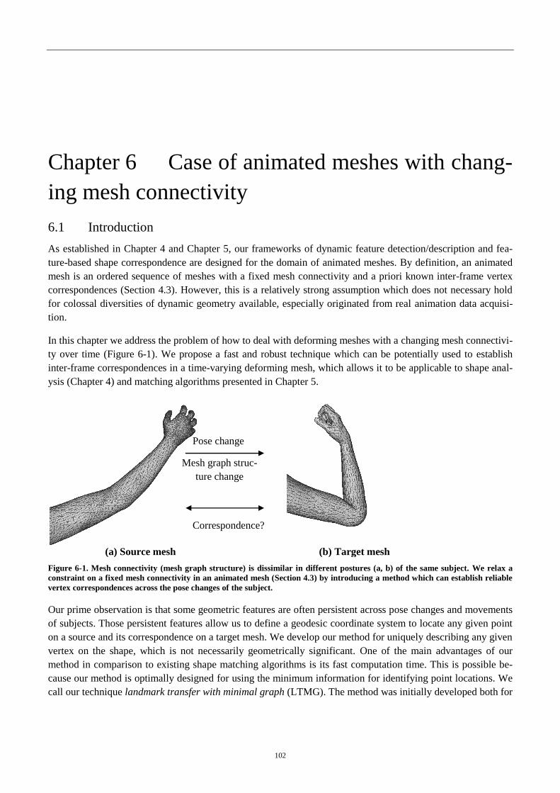
102

Chapter 6 Case of animated meshes with chang-

ing mesh connectivity

6.1 Introduction

As established in Chapter 4 and Chapter 5, our frameworks of dynamic feature detection/description and fea-

ture-based shape correspondence are designed for the domain of animated meshes. By definition, an animated

mesh is an ordered sequence of meshes with a fixed mesh connectivity and a priori known inter-frame vertex

correspondences (Section 4.3). However, this is a relatively strong assumption which does not necessary hold

for colossal diversities of dynamic geometry available, especially originated from real animation data acquisi-

tion.

In this chapter we address the problem of how to deal with deforming meshes with a changing mesh connectivi-

ty over time (Figure 6-1). We propose a fast and robust technique which can be potentially used to establish

inter-frame correspondences in a time-varying deforming mesh, which allows it to be applicable to shape anal-

ysis (Chapter 4) and matching algorithms presented in Chapter 5.

(a) Source mesh (b) Target mesh

Figure 6-1. Mesh connectivity (mesh graph structure) is dissimilar in different postures (a, b) of the same subject. We relax a

constraint on a fixed mesh connectivity in an animated mesh (Section 4.3) by introducing a method which can establish reliable

vertex correspondences across the pose changes of the subject.

Our prime observation is that some geometric features are often persistent across pose changes and movements

of subjects. Those persistent features allow us to define a geodesic coordinate system to locate any given point

on a source and its correspondence on a target mesh. We develop our method for uniquely describing any given

vertex on the shape, which is not necessarily geometrically significant. One of the main advantages of our

method in comparison to existing shape matching algorithms is its fast computation time. This is possible be-

cause our method is optimally designed for using the minimum information for identifying point locations. We

call our technique landmark transfer with minimal graph (LTMG). The method was initially developed both for

Pose change

Mesh graph struc-

ture change

Correspondence?

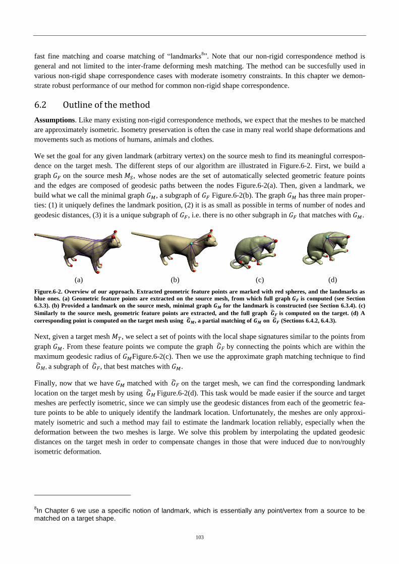
103

fast fine matching and coarse matching of “landmarks8”. Note that our non-rigid correspondence method is

general and not limited to the inter-frame deforming mesh matching. The method can be succesfully used in

various non-rigid shape correspondence cases with moderate isometry constraints. In this chapter we demon-

strate robust performance of our method for common non-rigid shape correspondence.

6.2 Outline of the method

Assumptions. Like many existing non-rigid correspondence methods, we expect that the meshes to be matched

are approximately isometric. Isometry preservation is often the case in many real world shape deformations and

movements such as motions of humans, animals and clothes.

We set the goal for any given landmark (arbitrary vertex) on the source mesh to find its meaningful correspon-

dence on the target mesh. The different steps of our algorithm are illustrated in Figure.6-2. First, we build a

graph on the source mesh , whose nodes are the set of automatically selected geometric feature points

and the edges are composed of geodesic paths between the nodes Figure.6-2(a). Then, given a landmark, we

build what we call the minimal graph , a subgraph of Figure.6-2(b). The graph has three main proper-

ties: (1) it uniquely defines the landmark position, (2) it is as small as possible in terms of number of nodes and

geodesic distances, (3) it is a unique subgraph of , i.e. there is no other subgraph in that matches with .

(a) (b) (c) (d)

Figure.6-2. Overview of our approach. Extracted geometric feature points are marked with red spheres, and the landmarks as

blue ones. (a) Geometric feature points are extracted on the source mesh, from which full graph is computed (see Section

6.3.3). (b) Provided a landmark on the source mesh, minimal graph for the landmark is constructed (see Section 6.3.4). (c)

Similarly to the source mesh, geometric feature points are extracted, and the full graph is computed on the target. (d) A

corresponding point is computed on the target mesh using , a partial matching of on (Sections 6.4.2, 6.4.3).

Next, given a target mesh , we select a set of points with the local shape signatures similar to the points from

graph . From these feature points we compute the graph by connecting the points which are within the

maximum geodesic radius of Figure.6-2(c). Then we use the approximate graph matching technique to find

, a subgraph of , that best matches with .

Finally, now that we have matched with on the target mesh, we can find the corresponding landmark

location on the target mesh by using Figure.6-2(d). This task would be made easier if the source and target

meshes are perfectly isometric, since we can simply use the geodesic distances from each of the geometric fea-

ture points to be able to uniquely identify the landmark location. Unfortunately, the meshes are only approxi-

mately isometric and such a method may fail to estimate the landmark location reliably, especially when the

deformation between the two meshes is large. We solve this problem by interpolating the updated geodesic

distances on the target mesh in order to compensate changes in those that were induced due to non/roughly

isometric deformation.

8In Chapter 6 we use a specific notion of landmark, which is essentially any point/vertex from a source to be

matched on a target shape.

104

6.3 Graph construction on the source mesh

6.3.1 Geodesic distance computation

Since our method relies heavily on the geodesic distance, its accurate computation is crucial. Later in this work,

geodesic distances are used to compute isocurves of the local descriptors on the surface (Section 6.3.2), as well

as to compute geodesic paths between geometric feature points (Section 6.3.3). Throughout this work, we adopt

the MMP method of exact geodesic computation proposed by (Mitchell, Mount, et al. 1987). The algorithm

itself is very similar to Dijkstra’s approximation on the graph formed by vertices and edges of the mesh. This

means that the surface of the mesh is regarded as locally planar on each face. As in Dijkstra’s algorithm we

start from a source vertex and compute the geodesic distance map in a region growing manner. Each edge in

the graph representation of the mesh is subdivided into a set of segments by artificially adding vertices on the

edge; on each Dijkstra’s step, when updating the geodesic map, a geodesic path is allowed to pass through these

artificial vertices. When there is no edge partitioning, we get standard Dijkstra’s algorithm; the more partition-

ing vertices go through, the more precise is the geodesics computation. In the worst case the algorithm has time

complexity . Note that the partial computation is possible: we can stop computation when the

path reaches certain distance or covers certain points on the surface of the mesh. This is an important point to

reduce the computation time.

6.3.2 Feature point extraction

We use a local static shape descriptor to identify the geometric features. Assuming approximate isometry be-

tween the source and target shapes, we are interested in a descriptor invariant to isometry and insensitive to the

mesh discretization as much as possible. We employ the intrinsic wave descriptor proposed by (Tevs, Berner et

al. 2011) and further refine it so that it is more robust to changes in mesh sampling.

For each vertex x we compute a set of intrinsic geodesic isocurves of increasing the geodesic distance from x

with a fixed step , by using the algorithm described in section 6.3.1. The length of each curve is then nor-

malized by , the length of the geodesic isocurve on a flat surface. We sampled 16 isocurves as in (Tevs,

Berner et al. 2011), resulting in the descriptor of a form

We approximate as a

perimeter of a polygon whose edges connect intersection points of the real isocurve with triangle edges on

the mesh. Next we take the inverse of the Euclidean norm of in order to measure the geometric prominence

(convexity/concavity) of vertex :

. (6-1)

Convexity increases with growing "sharpness" of the shape in the neighborhood of . Eventually comes

up to infinitely large values for a vertex on the tip of an infinitely sharp, needle-like shape.

Having computed the convexity all over the whole of the mesh (Figure. 6-3(a)), we sort its values in a

descending order and retain only the first vertices with the highest values of , with being the number of

vertices in the mesh. This gives us a set of most prominent vertices with respect to convexity. We normally

set a user-defined parameter with a value of 0.3. As can be seen from Figure. 6-3(b), the vertices from

group around ‘tips’ of the mesh; we denote the number of these clusters as .

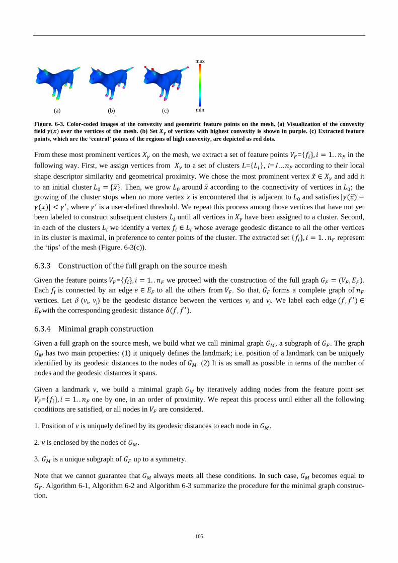
105

(a) (b) (c)

max

min

Figure. 6-3. Color-coded images of the convexity and geometric feature points on the mesh. (a) Visualization of the convexity

field over the vertices of the mesh. (b) Set of vertices with highest convexity is shown in purple. (c) Extracted feature

p ts, w c r t ‘c tr ’ p ts f the regions of high convexity, are depicted as red dots.

From these most prominent vertices on the mesh, we extract a set of feature points ={ in the

following way. First, we assign vertices from to a set of clusters L={ }, i=1… according to their local

shape descriptor similarity and geometrical proximity. We chose the most prominent vertex and add it

to an initial cluster . Then, we grow around according to the connectivity of vertices in ; the

growing of the cluster stops when no more vertex x is encountered that is adjacent to and satisfies

, where is a user-defined threshold. We repeat this process among those vertices that have not yet

been labeled to construct subsequent clusters until all vertices in have been assigned to a cluster. Second,

in each of the clusters we identify a vertex whose average geodesic distance to all the other vertices

in its cluster is maximal, in preference to center points of the cluster. The extracted set { represent

the ‘tips’ of the mesh (Figure. 6-3(c)).

6.3.3 Construction of the full graph on the source mesh

Given the feature points ={ we proceed with the construction of the full graph

Each is connected by an edge to all the others from . So that, forms a complete graph of

vertices. Let (vi, vj) be the geodesic distance between the vertices vi and vj. We label each edge

with the corresponding geodesic distance .

6.3.4 Minimal graph construction

Given a full graph on the source mesh, we build what we call minimal graph , a subgraph of . The graph

has two main properties: (1) it uniquely defines the landmark; i.e. position of a landmark can be uniquely

identified by its geodesic distances to the nodes of . (2) It is as small as possible in terms of the number of

nodes and the geodesic distances it spans.

Given a landmark v, we build a minimal graph by iteratively adding nodes from the feature point set

={ one by one, in an order of proximity. We repeat this process until either all the following

conditions are satisfied, or all nodes in are considered.

1. Position of v is uniquely defined by its geodesic distances to each node in .

2. v is enclosed by the nodes of .

3. is a unique subgraph of up to a symmetry.

Note that we cannot guarantee that always meets all these conditions. In such case, becomes equal to

Algorithm 6-1, Algorithm 6-2 and Algorithm 6-3 summarize the procedure for the minimal graph construc-

tion.

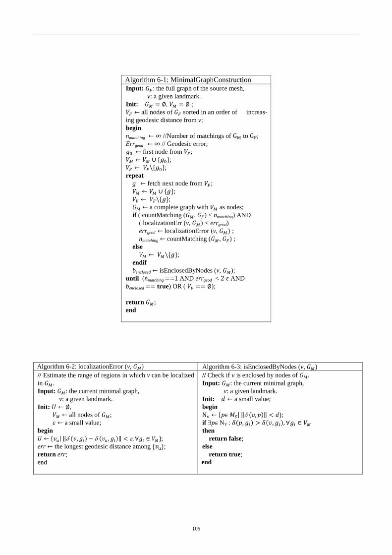
106

Algorithm 6-1: MinimalGraphConstruction

Input: : the full graph of the source mesh,

v: a given landmark.

Init: , ;

all nodes of sorted in an order of increas-

ing geodesic distance from v;

begin

nmatching //Number of matchings of to ;

Errgeod // Geodesic error;

first node from ;

; ; repeat

g fetch next node from ;

; ; a complete graph with as nodes;

if ( countMatching ( , ) < nmatching) AND

( localizationErr (v, < errgeod)

errgeod localizationError (v, ; nmatching countMatching ( , ) ;

else

; endif

benclosed isEnclosedByNodes (v, );

until (nmatching 1 AND errgeod < AND

benclosed true) OR ( );

return ;

end

Algorithm 6-2: localizationError (v, ) Algorithm 6-3: isEnclosedByNodes (v, )

// Estimate the range of regions in which v can be localized

in .

Input: : the current minimal graph,

v: a given landmark.

Init: ,

all nodes of ;

a small value;

begin

;

err the longest geodesic distance among ; return err;

end

// Check if v is enclosed by nodes of .

Input: : the current minimal graph,

v: a given landmark.

Init: a small value;

begin

;

if p NV :

then

return false;

else

return true;

end

107

Unique coordinates condition. Let ={ be the set of nodes of . We first find the set of

all vertices whose geodesic distances to are of approximately equal length to those of v, as represented by:

, (6-2)

where is a distances tolerance of equal geodesic length. If the largest geodesic distance among the vertices in

is smaller than , we consider that satisfies the unique coordinates condition, i.e. it can accurately lo-

cate v (see Figure. 6-4).

(a) (b)

(v, gA)

v

(v, gB)

(v, gB) (v, gA)

gA gB

v

(v, gC)

(v, gA) (v, gB)

v gC

gA gB

Figure. 6-4. Construction of the minimal graph. (a) By using two feature points (white dots), there are two possible position of

landmark (black dot), thus the landmark is not uniquely defined. value from is large. (b) With a minimal graph composed of

three feature points, the landmark position is more unique ( is very localized and is small).

Enclose-by-nodes condition. The second condition requires v to be enclosed by the nodes of , which makes

the localization of v more robust to small changes of geodesic distances. In Figure. 6-5(a), feature points gA, gB

and gC are located on one (the left) side of the landmark v. When the geodesic distances (v, gA), (v, gB) and

(v, gC) increase or decrease with the deformation, the estimated position of v will move to right or left, respec-

tively. In Figure. 6-5(b), on the other hand, by using additional feature point gD located on the other side of v,

the distance changes influenced by (v, gA), (v, gB) and (v, gC) will counterbalance with the change of (v, gD).

This strategy assumes simultaneous increase or decrease of geodesic distances, which has been usually the case

in our experiments.

(a) (b)

gA

gB

gC

v

gA

gB

gC

v

gD

Figure. 6-5. (a), the landmark (dark dot) is not surrounded by feature points (white dots). In (b), by adding another feature

point, the landmark is inside a convex hull; increases the confidence in the localization of the landmark.

The algorithm proceeds as follows. First, we compute a set NV of all the vertices in the neighborhood (within

certain geodesic distance) of v. If there exists a point p NV which is located further (with respect to v) to all the

nodes of , then does not satisfy the enclose-by-nodes condition with respect to v.

Unique subgraph condition. Primary step of our minimal graph construction algorithm is to ensure that the

landmark is defined uniquely on the source mesh. Several possible matching between and implies mul-

tiple matching between and , and therefore multiple transferred landmarks that are computed from each

matching. In order to avoid such an ambiguity, we build as a unique subgraph of .

108

We initially tried to check the number of matching of the minimal graph with the full graph at each iteration,

and stop growing the graph when we find only one matching. The graph matching algorithm we use is develo-

ped in spirit of Ullmann’s tree-search subgraph isomorphism (Ullmann 1976), which we describe in (

109

Appendix B : Subgraph matching using Ullmann's Algorithm). However, in the presence of symmetry in the

mesh, which is often the case, the minimal graph will always be equal to the full graph, which is undesirable.

Thus, we slightly modify our initial algorithm and add vertices to the current minimal graph only when the

resulting graph reduces the number of matching to the full graph. This means that the our method does not gua-

ranty the uniqueness of the matching of the minimal graph to the full graph, permitting the symmetric ambigui-

ty. Further discussions related to this aspect can be found in Section 6.5.5.

6.4 Landmark transfer via graph matching

6.4.1 Construction of the full graph on the target mesh

Similarly to the source, we first extract the feature points on the target mesh using the convexity values com-

puted from the modified intrinsic wave descriptor (Section 6.3.2). These feature points constitute the nodes of

, the full graph on the target mesh. To distinguish target mesh structures from the counterparts of the source,

we use a ‘hat’ notation. Next, we compute the geodesic paths among them which serve as weighted edges of .

We avoid computing all the geodesic paths by limiting ourselves to those geodesic paths on the target mesh

whose length is smaller or equal to lmax, the longest geodesic distance in . An explanation for this is that

paths that exceed lmax will obviously not match with any path of the minimal graph .

6.4.2 Matching the minimal graph to the full graph

Having computed , our goal now is to find a subgraph of , that best matches with . In general, due

to imperfect isometries in the real world data sets, full graphs might not be consistent across the given meshes.

We handle this problem again by using a variant of Ullmann’s graph matching algorithm (Ullmann 1976) (see

Appendix B for a detailed description), with partial matching. This time, while building a search tree of possi-

ble matching solutions we consider partial matching as well, i.e. we look for a subgraph of which is iso-

morphic to some subgraph of . For each possible matching an error value is assigned, and the matching with

the minimal error is chosen as the solution =( ), which is then used to locate the landmark on the tar-

get mesh.

Note that instead of relying on modified Ullmann’s graph matching algorithm (Ullmann 1976), any inexact

sub-graph matching approaches can be adopted such as (Torresani, Kolmogorov 2013). However, since the size

of our graphs in most of the cases does not exceed ten nodes we decided to stick to the plain graph matching

algorithm because there is no practical reason to use complex graph matching solutions, which might be inter-

esting in the case of larger and less coherent graphs.

6.4.3 Landmark transfer

If the source mesh and target mesh are perfectly isometric, then we are able to uniquely identify the

landmark location by using solely the geodesic distances from each of the nodes of . Let us denote a set of

geodesic distances from a vertex v to the vertices from , as

,

(6-3)

and refer to it as feature point coordinates of v (FP-coordinates). Then, we must be able to uniquely determine

the location of the transferred point on that satisfies

where

. (6-4)

110

However, in practice, and are not isometric and in general case

. This is partly due to

the definition of the geodesic distance (Bose, Maheshwari et al. 2011), the shortest surface distance between the

two points. As illustrated in Figure. 6-6, the shortest geodesic path between the two points of interest changes

as the shape deforms. Along the bending of the cylinder, we observed up to 9% of change in the geodesic dis-

tances.

u

v

u

v

Figure. 6-6. A simple illustration of influence of pose change on the geodesic path between given points. The geodesic path as

well as its distance between u and v change with the mesh deformation, from 100 to 90.7.

Our solution to the above problem is to modify the geodesic distances on the target mesh in a way that they

become similar to those of the source mesh. Let , , , be two feature points on the target mesh and their

corresponding counterpart on the source mesh respectively. Due to the non-isometric deformation, the distances

are different from , with and being a vertex on the source mesh and its counterpart on the

target mesh respectively. The idea is to modify the all geodesic distances from such that these geodesic dis-

tances become closer to those of the source mesh. That is, the distance will become equal to .

Similarly, the distance of vertex v in the close neighborhood of (i.e. ) will be

become close to .

Computation of the feature point coordinates using inverse distance weighting (IDW). Let be a vertex

of the minimal graph on the source mesh and its counterpart on the target mesh. We compute the geodesic

distance histogram of these two vertices. The geodesic distance histogram describes the distribution of

the geodesic distances between the vertex and all the other vertices of the mesh . As illustrated in Figure.

6-7, the histograms and might be dissimilar, although and are the same point on the shape.

The main idea is to modify the geodesic distances of such that the histogram becomes similar

to . This is done by using the inverse distance weighting method and the geodesic distances of the mini-

mal graph vertices.

We define the interpolated geodesic distance by means of inverse distance weighting:

=

(6-5)

where =

.

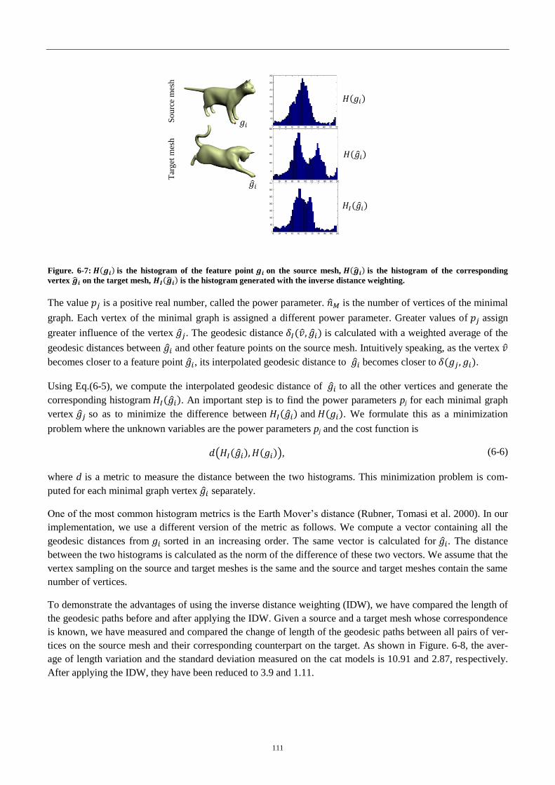
111

Figure. 6-7: is the histogram of the feature point on the source mesh, is the histogram of the corresponding

vertex on the target mesh, is the histogram generated with the inverse distance weighting.

The value is a positive real number, called the power parameter. is the number of vertices of the minimal

graph. Each vertex of the minimal graph is assigned a different power parameter. Greater values of assign

greater influence of the vertex . The geodesic distance is calculated with a weighted average of the

geodesic distances between and other feature points on the source mesh. Intuitively speaking, as the vertex

becomes closer to a feature point , its interpolated geodesic distance to becomes closer to .

Using Eq.(6-5), we compute the interpolated geodesic distance of to all the other vertices and generate the

corresponding histogram . An important step is to find the power parameters pj for each minimal graph

vertex so as to minimize the difference between and . We formulate this as a minimization

problem where the unknown variables are the power parameters pj and the cost function is

, (6-6)

where d is a metric to measure the distance between the two histograms. This minimization problem is com-

puted for each minimal graph vertex separately.

One of the most common histogram metrics is the Earth Mover’s distance (Rubner, Tomasi et al. 2000). In our

implementation, we use a different version of the metric as follows. We compute a vector containing all the

geodesic distances from sorted in an increasing order. The same vector is calculated for . The distance

between the two histograms is calculated as the norm of the difference of these two vectors. We assume that the

vertex sampling on the source and target meshes is the same and the source and target meshes contain the same

number of vertices.

To demonstrate the advantages of using the inverse distance weighting (IDW), we have compared the length of

the geodesic paths before and after applying the IDW. Given a source and a target mesh whose correspondence

is known, we have measured and compared the change of length of the geodesic paths between all pairs of ver-

tices on the source mesh and their corresponding counterpart on the target. As shown in Figure. 6-8, the aver-

age of length variation and the standard deviation measured on the cat models is 10.91 and 2.87, respectively.

After applying the IDW, they have been reduced to 3.9 and 1.11.

So

urc

e m

esh

Tar

get

mes

h

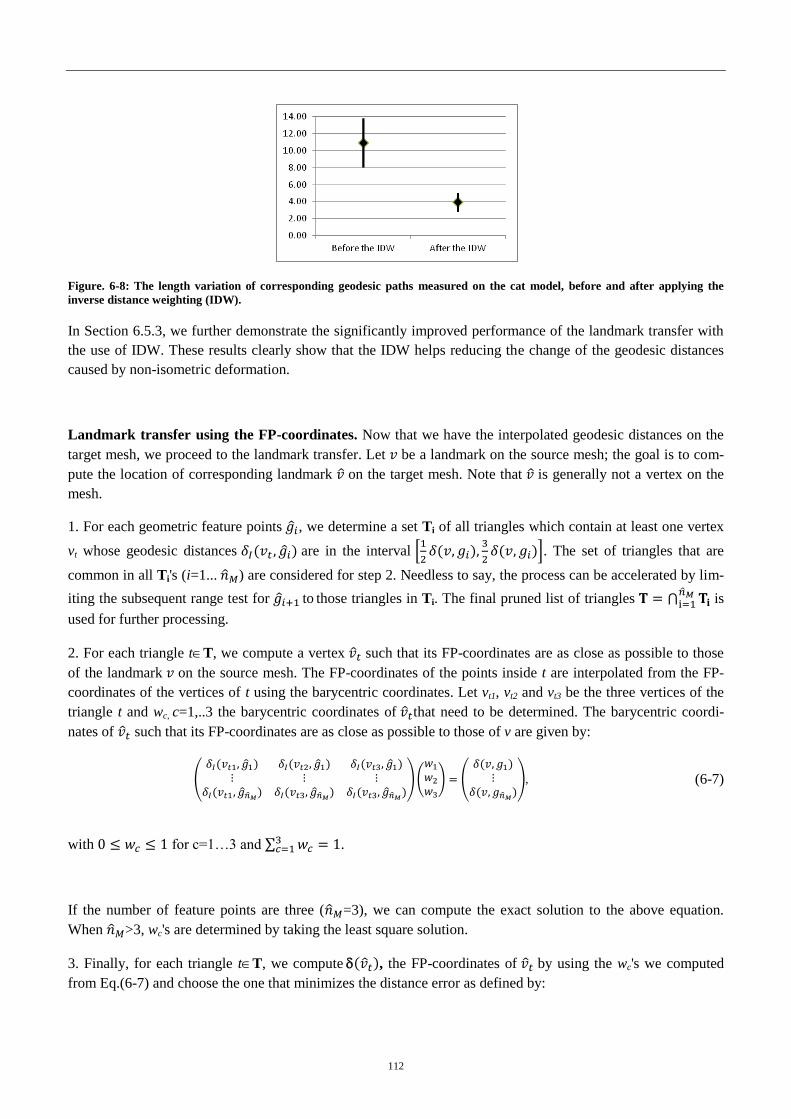
112

Figure. 6-8: The length variation of corresponding geodesic paths measured on the cat model, before and after applying the

inverse distance weighting (IDW).

In Section 6.5.3, we further demonstrate the significantly improved performance of the landmark transfer with

the use of IDW. These results clearly show that the IDW helps reducing the change of the geodesic distances

caused by non-isometric deformation.

Landmark transfer using the FP-coordinates. Now that we have the interpolated geodesic distances on the

target mesh, we proceed to the landmark transfer. Let be a landmark on the source mesh; the goal is to com-

pute the location of corresponding landmark on the target mesh. Note that is generally not a vertex on the

mesh.

1. For each geometric feature points , we determine a set Ti of all triangles which contain at least one vertex

vt whose geodesic distances are in the interval

. The set of triangles that are

common in all Ti's (i=1... ) are considered for step 2. Needless to say, the process can be accelerated by lim-

iting the subsequent range test for to those triangles in Ti. The final pruned list of triangles is

used for further processing.

2. For each triangle t T, we compute a vertex such that its FP-coordinates are as close as possible to those

of the landmark on the source mesh. The FP-coordinates of the points inside t are interpolated from the FP-

coordinates of the vertices of t using the barycentric coordinates. Let vt1, vt2 and vt3 be the three vertices of the

triangle t and wc, c=1,..3 the barycentric coordinates of that need to be determined. The barycentric coordi-

nates of such that its FP-coordinates are as close as possible to those of v are given by:

, (6-7)

with for c=1…3 and .

If the number of feature points are three ( =3), we can compute the exact solution to the above equation.

When >3, wc's are determined by taking the least square solution.

3. Finally, for each triangle t T, we compute , the FP-coordinates of by using the wc's we computed

from Eq.(6-7) and choose the one that minimizes the distance error as defined by:

113

. (6-8)

6.5 Results

In this section, we present results of experiments with the method described in the preceding sections. We im-

plemented our algorithm using Matlab. All measurements were made on a Windows 7 Professional machine

with 16GB of memory and Intel Core i7-2600 processor running at 3.40 GHz. We tested our method on the

models of different mesh connectivity (Figure 6-9) from the Non-Rigid World Benchmark (Bronstein A., Bron-

stein M. et al. 2008), as well as on our own synthetic embossed plate models.

Figure 6-11 shows some of the results we obtained. Note that these models exhibit deformations which are only

approximate isometries; also each family of objects have a mesh in an initial posture, which is labelled as a

mesh in a rest posture (or source mesh). The landmarks have been chosen to be a set of 100 points evenly

spaced over the surface using Poisson sampling. In order to avoid repetitive computation of the graph matching,

the minimal graph is set to the full graph, so that, the graph matching is computed only once for the transfer of

the 100 points. Compared to the minimal graph method, the computation time is about 2 to 3 times higher. We

conducted a series of experiments and applied our algorithm to all the vertices in Poisson sampling sets. The

quality of transfer is compared with the ground-truth correspondences from high-resolution Tosca models

(Figure. 6-12), and with correspondences computed with existing methods (see Section 6.5.4).

(a) (b)

Figure 6-9. The models we used in our experiments have different number of vertices and mesh connec-

tivity. (a) Centaur mesh comprised of 7K vertices. (b) Centaur mesh in different posture comprised of

5K of vertices.

6.5.1 Timing

In Table 6-1 an average computation time is shown, which was measured while transferring each of the land-

marks; the time was measured and then averaged over landmark transfer to 10 cat models, 6 centaur models, 8

dog models, and 3 embossed plate models. We clearly see that the computation of the updated geodesic dis-

tances (see Section 6.4.3) is the most time-consuming task. However, an update of the geodesic distances ac-

cording to the histograms (see Figure. 6-7) is required only once per each target mesh. That is, it does not mat-

ter how many landmarks are to be transferred from the source to the target (e.g. 10 or 103), the geodesics are

updated only once. i.e. it makes our technique very efficient when working with a number of landmarks. For

example, once the geodesic distances are updated, it takes only 256ms to transfer a landmark on the cat model

(Table 6-1).

114

Data set +

Cat 4K 9K 146ms 21ms 39ms 59ms 6.63s

Centaur 5K 10K 86ms 23ms 128ms 338ms 48.96s

Dog 5K 9.5K 104ms 20ms 33ms 39ms 5.98s

Embossed plate 1.5K 2.9K 19ms 7ms 85ms 1708ms 2.81s

Table 6-1: Average computation time. is the average number of vertices over all postures, and is the average number of

triangles, is the average time needed to compute the geodesic distance matrix per each vertex, is the average time needed to

extract feature points, is the average time needed to build a minimal graph, is the average time for updating the geodesic

distances; hat over a symbol refers to it the target mesh.

As shown in Table 6-1, the overall time of landmark transfer is just a matter of seconds; except for the centaur

model. On the centaur our method shows rather a high computation time. The main reason is that this mesh has

many more geometric feature points compared to other models (e.g. 15 feature points for the centaur vs. only 8

for the cat). Since is a function of a number of vertices and geometric features, our technique works fast on

the embossed plate, which also has many geometric features, but the number of vertices is much less compared

to the centaur model. In general, the computation time is an advantage of our method. It takes about 1 minute to

find full correspondence for the cat model (on Matlab platform). This has been possible because (1) the update

of the geodesic distances has been made only once, and (2) full graph has been used in place of minimal graph

for every vertex.

6.5.2 Robustness

Minimal graph plays one of the central roles in our landmark transfer algorithm; and naturally, the quality of

transfer is correlated to the selection of . In Figure. 6-10 (a, b) is shown a case when the landmark was

picked at the base of a human neck, which is close to the geometric feature points on the head, breast and hands.

With such settings our minimal graph construction algorithm gives a compact . On the other hand, when the

landmark is located far away from geometric feature points, as in Figure. 6-10 (c, d), turns out to be ‘large’

in terms of the geodesic distances of the edges. A ‘small’ minimal graph is preferred in our algorithm. First

reason for this is that the shorter the graph edges are, the less distortion and error is introduced for correspond-

ing graph on the other isometric mesh. Second, when is small, less geodesic computations are needed to

find corresponding one on the target. Note that by configuring a maximum size and number of isocurves of the

local shape descriptor, we can achieve detection of different number of feature points, according to our needs

and mesh complexity. In our experiment, we were able to extract from just a few to dozens of feature points on

the same human model.

(a) (b) (c) (d)

Figure. 6-10. Impact of the landmark location on the quality of transfer and performance. (a), (b) Landmark on the neck is

closely surrounded by feature points. (c),(d) Landmark in the belly area has relatively large average distance to the feature

points of the surface.

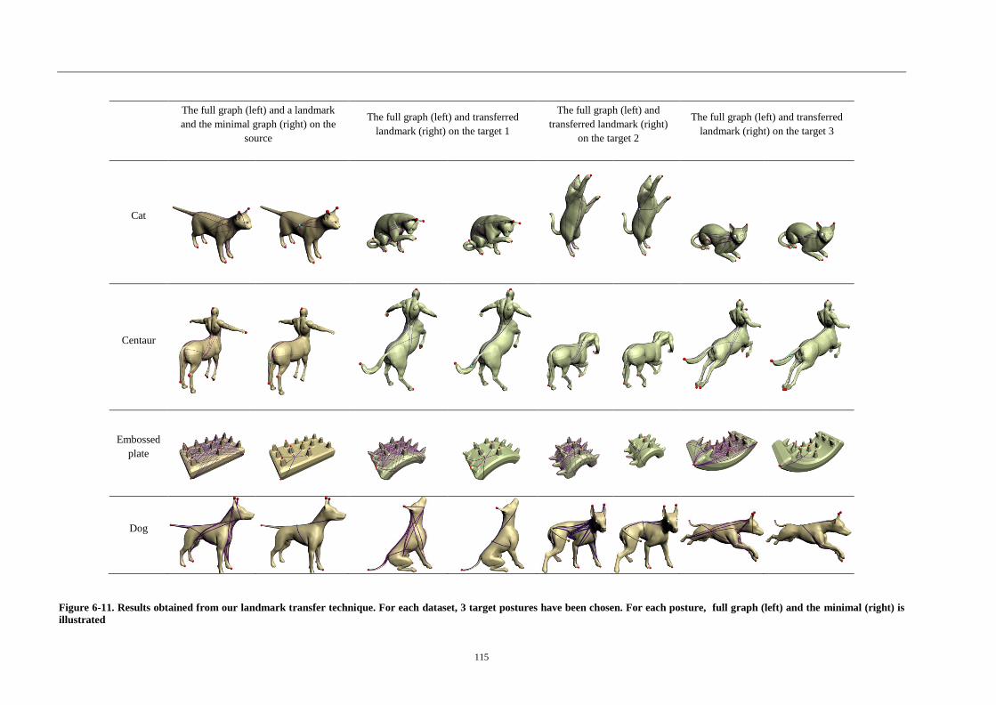
115

The full graph (left) and a landmark

and the minimal graph (right) on the

source

The full graph (left) and transferred

landmark (right) on the target 1

The full graph (left) and

transferred landmark (right)

on the target 2

The full graph (left) and transferred

landmark (right) on the target 3

Cat

Centaur

Embossed

plate

Dog

Figure 6-11. Results obtained from our landmark transfer technique. For each dataset, 3 target postures have been chosen. For each posture, full graph (left) and the minimal (right) is

illustrated

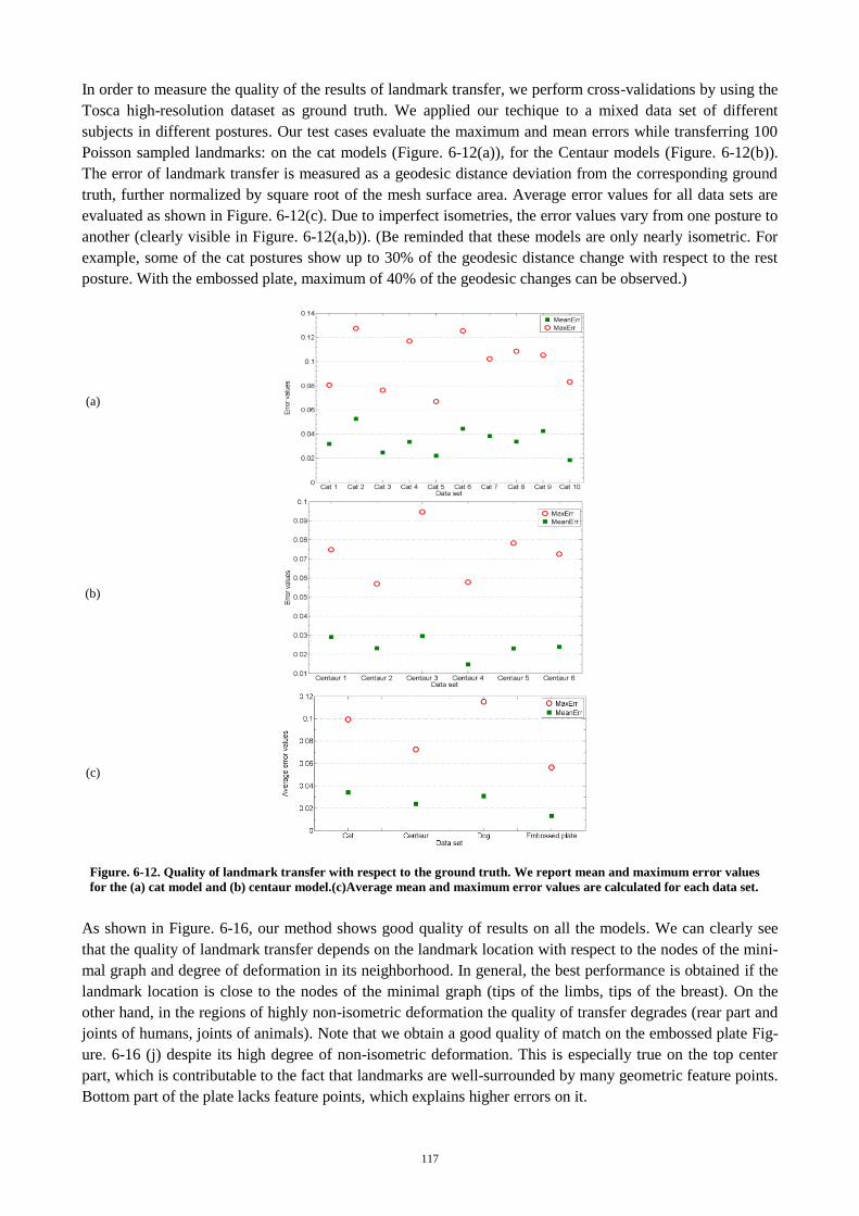
117

In order to measure the quality of the results of landmark transfer, we perform cross-validations by using the

Tosca high-resolution dataset as ground truth. We applied our techique to a mixed data set of different

subjects in different postures. Our test cases evaluate the maximum and mean errors while transferring 100

Poisson sampled landmarks: on the cat models (Figure. 6-12(a)), for the Centaur models (Figure. 6-12(b)).

The error of landmark transfer is measured as a geodesic distance deviation from the corresponding ground

truth, further normalized by square root of the mesh surface area. Average error values for all data sets are

evaluated as shown in Figure. 6-12(c). Due to imperfect isometries, the error values vary from one posture to

another (clearly visible in Figure. 6-12(a,b)). (Be reminded that these models are only nearly isometric. For

example, some of the cat postures show up to 30% of the geodesic distance change with respect to the rest

posture. With the embossed plate, maximum of 40% of the geodesic changes can be observed.)

(a)

(b)

(c)

Figure. 6-12. Quality of landmark transfer with respect to the ground truth. We report mean and maximum error values

for the (a) cat model and (b) centaur model.(c)Average mean and maximum error values are calculated for each data set.

As shown in Figure. 6-16, our method shows good quality of results on all the models. We can clearly see

that the quality of landmark transfer depends on the landmark location with respect to the nodes of the mini-

mal graph and degree of deformation in its neighborhood. In general, the best performance is obtained if the

landmark location is close to the nodes of the minimal graph (tips of the limbs, tips of the breast). On the

other hand, in the regions of highly non-isometric deformation the quality of transfer degrades (rear part and

joints of humans, joints of animals). Note that we obtain a good quality of match on the embossed plate Fig-

ure. 6-16 (j) despite its high degree of non-isometric deformation. This is especially true on the top center

part, which is contributable to the fact that landmarks are well-surrounded by many geometric feature points.

Bottom part of the plate lacks feature points, which explains higher errors on it.

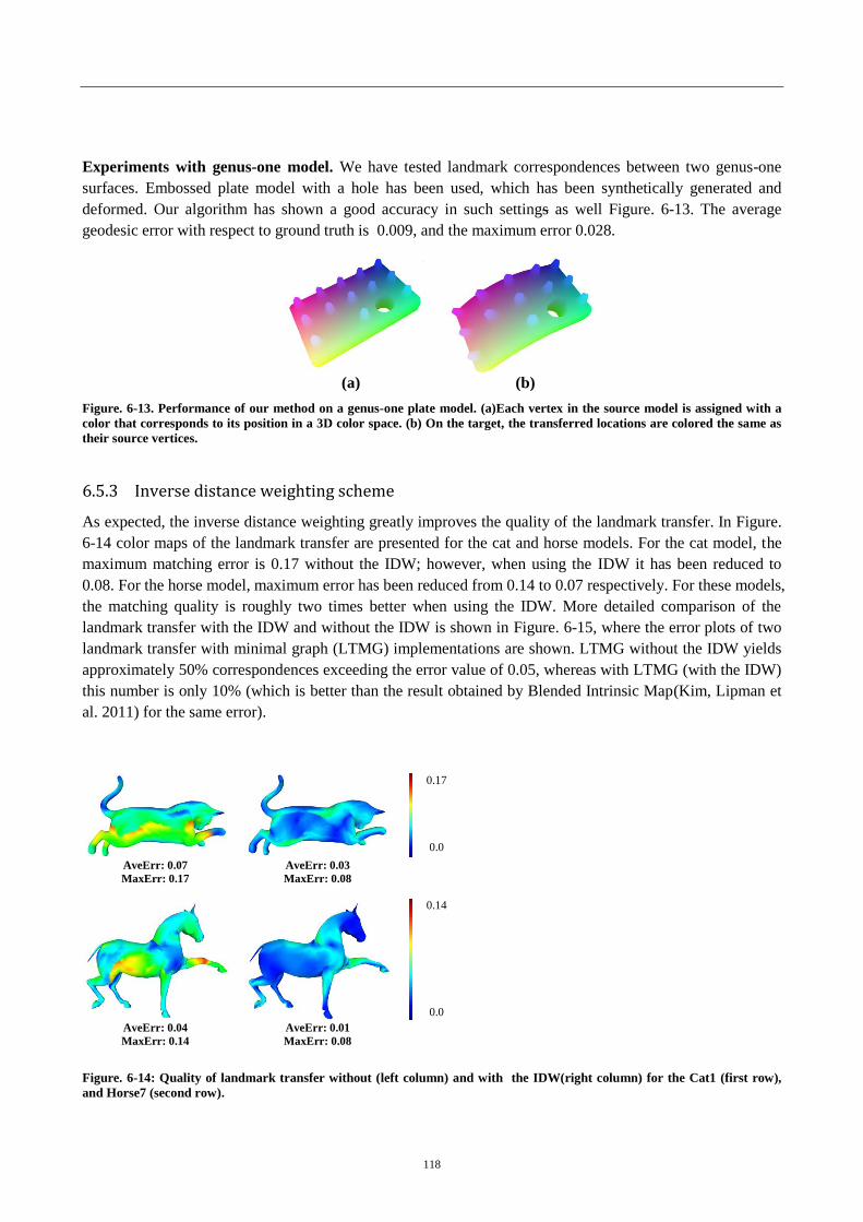
118

Experiments with genus-one model. We have tested landmark correspondences between two genus-one

surfaces. Embossed plate model with a hole has been used, which has been synthetically generated and

deformed. Our algorithm has shown a good accuracy in such settings as well Figure. 6-13. The average

geodesic error with respect to ground truth is 0.009, and the maximum error 0.028.

(a) (b)

Figure. 6-13. Performance of our method on a genus-one plate model. (a)Each vertex in the source model is assigned with a

color that corresponds to its position in a 3D color space. (b) On the target, the transferred locations are colored the same as

their source vertices.

6.5.3 Inverse distance weighting scheme

As expected, the inverse distance weighting greatly improves the quality of the landmark transfer. In Figure.

6-14 color maps of the landmark transfer are presented for the cat and horse models. For the cat model, the

maximum matching error is 0.17 without the IDW; however, when using the IDW it has been reduced to

0.08. For the horse model, maximum error has been reduced from 0.14 to 0.07 respectively. For these models,

the matching quality is roughly two times better when using the IDW. More detailed comparison of the

landmark transfer with the IDW and without the IDW is shown in Figure. 6-15, where the error plots of two

landmark transfer with minimal graph (LTMG) implementations are shown. LTMG without the IDW yields

approximately 50% correspondences exceeding the error value of 0.05, whereas with LTMG (with the IDW)

this number is only 10% (which is better than the result obtained by Blended Intrinsic Map(Kim, Lipman et

al. 2011) for the same error).

0.17

0.0 AveErr: 0.07

MaxErr: 0.17

AveErr: 0.03

MaxErr: 0.08

0.14

0.0

AveErr: 0.04

MaxErr: 0.14

AveErr: 0.01

MaxErr: 0.08

Figure. 6-14: Quality of landmark transfer without (left column) and with the IDW(right column) for the Cat1 (first row),

and Horse7 (second row).

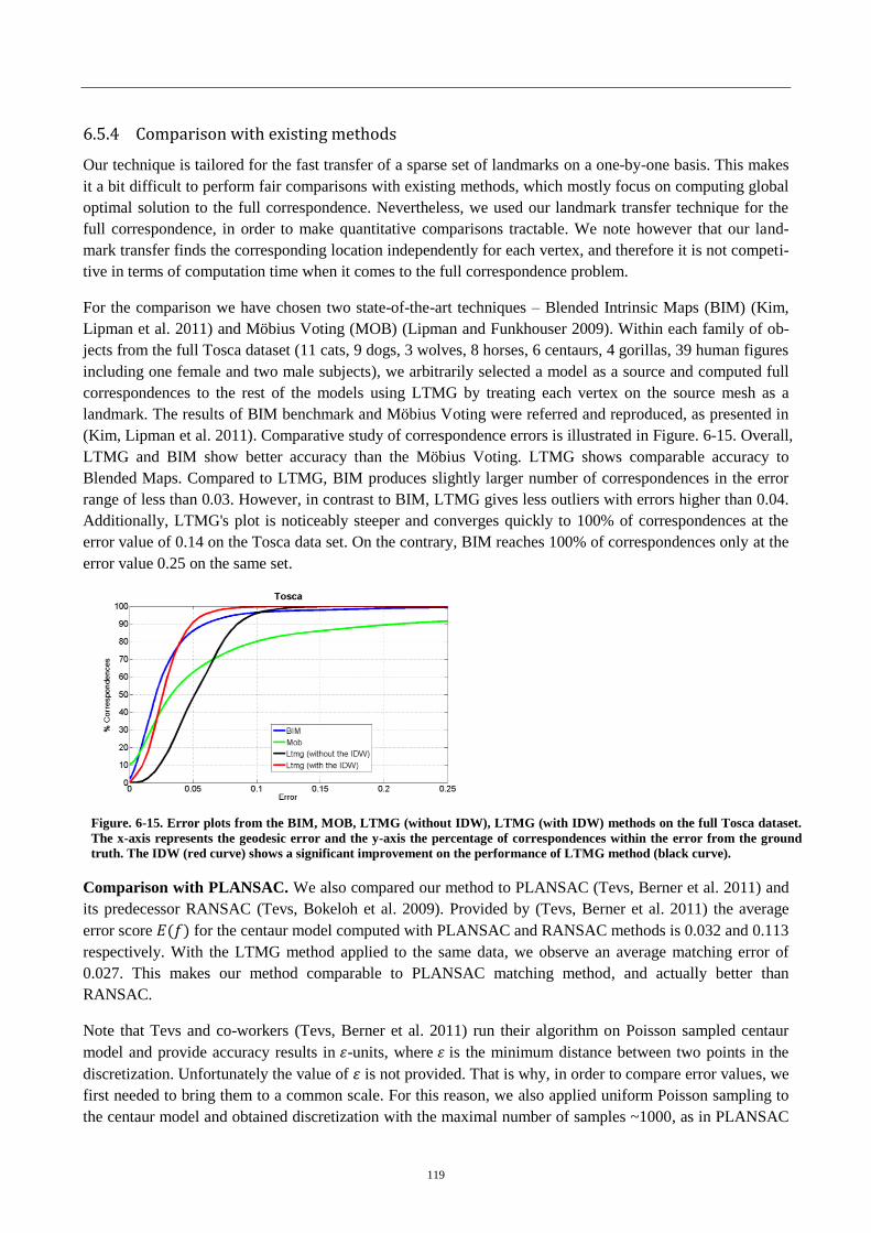
119

6.5.4 Comparison with existing methods

Our technique is tailored for the fast transfer of a sparse set of landmarks on a one-by-one basis. This makes

it a bit difficult to perform fair comparisons with existing methods, which mostly focus on computing global

optimal solution to the full correspondence. Nevertheless, we used our landmark transfer technique for the

full correspondence, in order to make quantitative comparisons tractable. We note however that our land-

mark transfer finds the corresponding location independently for each vertex, and therefore it is not competi-

tive in terms of computation time when it comes to the full correspondence problem.

For the comparison we have chosen two state-of-the-art techniques – Blended Intrinsic Maps (BIM) (Kim,

Lipman et al. 2011) and Möbius Voting (MOB) (Lipman and Funkhouser 2009). Within each family of ob-

jects from the full Tosca dataset (11 cats, 9 dogs, 3 wolves, 8 horses, 6 centaurs, 4 gorillas, 39 human figures

including one female and two male subjects), we arbitrarily selected a model as a source and computed full

correspondences to the rest of the models using LTMG by treating each vertex on the source mesh as a

landmark. The results of BIM benchmark and Möbius Voting were referred and reproduced, as presented in

(Kim, Lipman et al. 2011). Comparative study of correspondence errors is illustrated in Figure. 6-15. Overall,

LTMG and BIM show better accuracy than the Möbius Voting. LTMG shows comparable accuracy to

Blended Maps. Compared to LTMG, BIM produces slightly larger number of correspondences in the error

range of less than 0.03. However, in contrast to BIM, LTMG gives less outliers with errors higher than 0.04.

Additionally, LTMG's plot is noticeably steeper and converges quickly to 100% of correspondences at the

error value of 0.14 on the Tosca data set. On the contrary, BIM reaches 100% of correspondences only at the

error value 0.25 on the same set.

Figure. 6-15. Error plots from the BIM, MOB, LTMG (without IDW), LTMG (with IDW) methods on the full Tosca dataset.

The x-axis represents the geodesic error and the y-axis the percentage of correspondences within the error from the ground

truth. The IDW (red curve) shows a significant improvement on the performance of LTMG method (black curve).

Comparison with PLANSAC. We also compared our method to PLANSAC (Tevs, Berner et al. 2011) and

its predecessor RANSAC (Tevs, Bokeloh et al. 2009). Provided by (Tevs, Berner et al. 2011) the average

error score for the centaur model computed with PLANSAC and RANSAC methods is 0.032 and 0.113

respectively. With the LTMG method applied to the same data, we observe an average matching error of

0.027. This makes our method comparable to PLANSAC matching method, and actually better than

RANSAC.

Note that Tevs and co-workers (Tevs, Berner et al. 2011) run their algorithm on Poisson sampled centaur

model and provide accuracy results in -units, where is the minimum distance between two points in the

discretization. Unfortunately the value of is not provided. That is why, in order to compare error values, we

first needed to bring them to a common scale. For this reason, we also applied uniform Poisson sampling to

the centaur model and obtained discretization with the maximal number of samples ~1000, as in PLANSAC

120

settings. With this sampling, we have estimated the exact value of . Further normalization by the square root

of the model's surface area has yielded directly comparable error values.

6.5.5 Limitations

The main limitation of our method is that it relies on the geometric features of the shape. If the shape does

not have any prominent geometric points, our method is not applicable (for instance, our technique will not

be able to give a result on a sphere model). The reason for this is that our technique relies on a local shape

descriptor to extract feature points, which are then used as nodes of full and minimal graphs.

Apart from this, isometry between the source and target meshes is one of the main assumptions used in our

landmark transfer. That is rather strong assumption, although it holds valid in many real-world situations of

matching 3D scan data. When the meshes come from different objects, this assumption is violated and pro-

posed method may not work well.

Handling the symmetry. In the presence of symmetry, the landmark transfer will propose only one of all

possible solutions. This is related to the uniqueness condition of our minimal graph construction, which fa-

vors light computation in graph growing and graph matching, at the cost of permitting matching ambiguity,

which is originated from the symmetry. Since our current implementation of minimal graph construction

algorithm does not differentiate between the two symmetric minimal graphs given the same (graph-) match-

ing error, sometimes the transferred landmark can be located at the mirror-reflection of the desired location

of the transferred landmark. However, it would be easy to extend our method in a way that all possible trans-

fers are proposed to the user. We can simply consider all matching of the minimal graph to the full graph on

the target, and compute landmark transfer from each minimal graph. The user will then choose either one or

all of them, depending on what s/he wants to have. Note that in our robustness tests, the matching (landmark

position) error has been measured on one half of the meshes, by considering one location and its reflective

symmetry as identical.

121

6.6 Conclusion

Isometry preserving deformations are frequently encountered in real life: articulated motions and majority of

human movements. In Chapter 6 we presented a landmark transfer technique that efficiently computes vertex

matching on a source (original posture) and target (posture change) meshes that are approximately isometric.

The key idea of our approach is to use the minimum amount of information in geodesic coordinates which is

sufficient for locating any given point on a source shape and efficient computing its correspondence on a

target shape (Sections 6.3-6.4).

The matching method detailed in this chapter brings several contributions:

1. The new idea of the minimal graph (Section 6.3), which characterizes location of any point on a shape and

is used for shape matching with minimal computation expenses.

2. Identification of vertex locations using a newly defined geodesic coordinates (Section 6.4). In contrast to

previous approaches, we do not rely solely on geodesic distances. Instead we develop a reliable method of

updating geodesic distances, which compensates well the distance changes due to imperfect isometry and

assures precise and consistent vertex correspondence.

Our method shows robust and precise matching result with a low computational time cost in a large number

of experiments and different data sets (Section 6.5). Although, we demonstrate the effective performance of

our matching method in cases of pose changes of the given subjects, it is possible to proceed in a similar way

for establishing inter-frame correspondences of deforming mesh with a time-varying mesh connectivity,

which we plan to carry out in future. Additionally, our method can be ideal for a sparse one-to-many shapes

matching. For instance, given a set of sparse landmarks, our algorithm can find precise correspondences on a

set of multiple meshes in a matter of seconds, avoiding abundant multiple full shape matching.

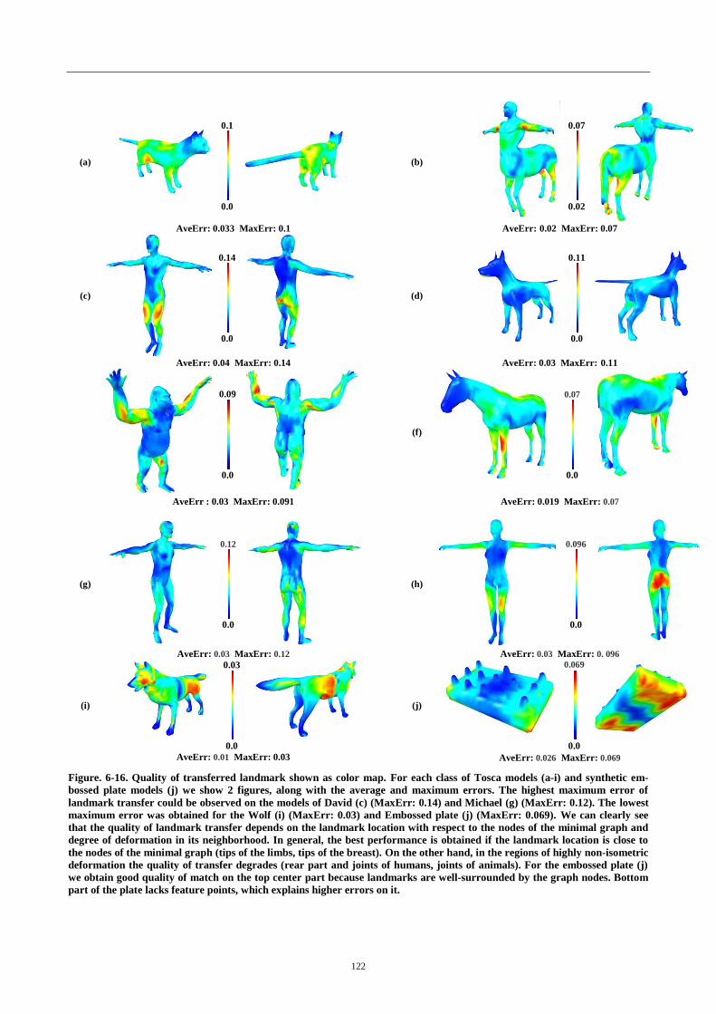
122

(a)

(b)

0.1 0.07

0.0 0.02

AveErr: 0.033 MaxErr: 0.1 AveErr: 0.02 MaxErr: 0.07

(c)

(d)

0.14 0.11

0.0 0.0

AveErr: 0.04 MaxErr: 0.14 AveErr: 0.03 MaxErr: 0.11

(f)

0.09 0.07

0.0 0.0

AveErr : 0.03 MaxErr: 0.091 AveErr: 0.019 MaxErr: 0.07

(g)

(h)

0.12 0.096

0.0 0.0

AveErr: 0.03 MaxErr: 0.12 AveErr: 0.03 MaxErr: 0. 096

(i)

0.03

(j)

0.069

0.0 0.0 AveErr: 0.01 MaxErr: 0.03 AveErr: 0.026 MaxErr: 0.069

Figure. 6-16. Quality of transferred landmark shown as color map. For each class of Tosca models (a-i) and synthetic em-

bossed plate models (j) we show 2 figures, along with the average and maximum errors. The highest maximum error of

landmark transfer could be observed on the models of David (c) (MaxErr: 0.14) and Michael (g) (MaxErr: 0.12). The lowest

maximum error was obtained for the Wolf (i) (MaxErr: 0.03) and Embossed plate (j) (MaxErr: 0.069). We can clearly see

that the quality of landmark transfer depends on the landmark location with respect to the nodes of the minimal graph and

degree of deformation in its neighborhood. In general, the best performance is obtained if the landmark location is close to

the nodes of the minimal graph (tips of the limbs, tips of the breast). On the other hand, in the regions of highly non-isometric

deformation the quality of transfer degrades (rear part and joints of humans, joints of animals). For the embossed plate (j)

we obtain good quality of match on the top center part because landmarks are well-surrounded by the graph nodes. Bottom

part of the plate lacks feature points, which explains higher errors on it.

123

Chapter 7 Conclusion

In this thesis, we have been interested in investigating shape analysis of time-varying geometry (i.e. ani-

mated meshes) and have presented novel algorithms for the dynamic feature detection, feature description on

animated meshes and their applications to shape correspondence. We paid a particular attention to the maxi-

mal use of dynamic motion properties in animated mesh sequences for dynamic feature point extraction and

description. Based on the dynamic features, we proposed a new pipeline of the shape correspondence based

on similarities of deformation properties of animated meshes rather than their purely static structures. On a

number of example animated meshes of drastically different shapes we demonstrated robustness and effi-

ciency of our surface deformation/motion-driven methods. Our approach is applicable to any deformations,

skeletal (humans/animals) or non-skeletal (faces). In Section 7.1 we highlight the contributions of this disser-

tation and in Section 7.2 we present several interesting future research directions.

7.1 Contributions

In this dissertation, we have focused our research on establishing correspondence computation pipeline be-

tween animated meshes by exploiting their surface deformation characteristics. Our work brings the follow-

ing prime contributions.

We presented a new feature detection technique on animated mesh sequences. First we started with a

local surface deformation characteristic scheme for animated meshes. Then we developed the core of

the proposed dynamic feature extraction technique which is formed by the principles of the linear

scale-space theory on animation’s deformation characteristics. Our contributions include: introduc-

tion of a new spatio-temporal scale representation of the animated mesh’s surface deformation, and

an extension of the classical DoG (Difference of Gaussians) filter to spatio-temporal case of ani-

mated meshes. Our method is able to robustly and repeatable extract consistent sets of feature points

over different deforming mesh surfaces. Validations and experiments on various types of data sets

show consistent feature extraction results when the exhibited animations are identical, kinematically

or semantically. Our approach has also shown robustness to spatial and temporal sampling of mesh

animation.

The main contribution of our work is a solid correspondence pipeline for animated meshes, featuring

new dynamic feature descriptors. It consolidates the new dynamic feature detection, dynamic feature

description, and sparse/dense point-to-point matching. The newly proposed dynamic point signature

comprised of different motion modalities and deformation properties of animated mesh. It has been

successfully adopted in efficient and precise coarse matching of dynamic feature points and conse-

quently has driven robust fine matching between different animated meshes. Additionally, our

method can help avoid symmetry confusion in matching of deforming meshes with the use of dy-

namic motion properties of the subject’s motion (The majority of real-world human or animal mo-

tions are asymmetric).

Finally, with an aim of finding inter-frame correspondence for animated meshes with the time vary-

ing mesh connectivity, we have developed an efficient and robust matching method for approxi-

mately isometric deformable shapes. The prime idea of the method is to use the minimal amount of

124

information to precisely locate a point location in geodesic coordinates on the source mesh and re-

construct its location on the target mesh. One of the major benefits of the method is a very light

computational time of the matching method when it comes to the matching of a few number of se-

lected points. Experiments on dense correspondence confirm that our technique shows a comparable

performance with respect to the state of the art matching algorithms.

7.2 Future directions

We believe that the methods studied in this dissertation bring a number of promising research directions and

interesting applications towards new contributions in analysis of time-varying geometry.

The outcome of the work conducted in scope of this dissertation suggests several new research paths.

Given the developments we produced in the scope of this dissertation, one interesting research direc-

tion would be a statistical shape analysis of animated meshes. It is reasonable to pose a question on

how existing shape analysis techniques based on statistical models (such as Anguelov, Srinivasan et

al. 2005) can be adapted to incorporate dynamic data. Indeed, statistical shape analysis of animated

mesh’s shapes and corresponding deformations has a tremendous potential. One way to proceed is to

set up a statistical model that captures both shape variations and deformation resulting from motions

of instances of distinct animations in an animated mesh database. Within the low dimensional statis-

tical model we can analyze the deformation properties involving different shape variations and dif-

ferent movements. The learnt animated mesh shape-deformation statistical model can be developed

into techniques for the improvement of shape correspondence methods in spirit of how it was previ-

ously done in statistical atlases for static shapes. Additionally, machine learning algorithms can be

applied to the full body time varying animation statistical model to enhance and contribute to the

methods of human modelling and animation.

We also consider improving the shape correspondence algorithms by capturing more mechanical

properties of the deforming surface in an animated mesh. A substantial amount of research in com-

puter graphics focuses on physic-based techniques. In real world, laws of physics govern motion and

deformation of objects and might become an integral component of shape correspondence pipeline.

Physic-based properties such as surface’s strain and stress tensors directions (so far in this disserta-

tion we have employed only magnitudes of strain tensors) can be eventually incorporated into the

shape correspondence technique. Physical, mechanical properties of the deforming shapes might be

further incorporated into dynamic feature vectors. One possible option can be to extract physical

properties of the regions of interest on the source and compare extracted deformation tensor field di-

rections to the ones estimated on the target animated mesh. Ultimately, the shape correspondence

can be posed as a global optimization which compares and aligns deformation tensor fields on the

surfaces of the source and target animated meshes.

Alternatively, dynamic feature points which are equipped with shape correspondence of animated

meshes can be employed in more pragmatic applications in medicine (i.e. deviations in movements

of internal organs) and sports (performance and motion analysis of athlete’s movements). For exam-

ple, the comparison studies of dynamic feature points extracted from the heart movement data of a

patient and a reference healthy heart can help clinicians to better understand and diagnose potential

abnormalities.

The principal idea of the geodesic graph-based surface representation from the landmark transfer al-

gorithm could be potentially adopted for challenging inter-frame correspondence problems in time-

varying geometry originating from optical sensors. Acquisition noise, holes etc. typically persist in

such data sets, which make geodesic paths not completely reliable on deforming shapes that have

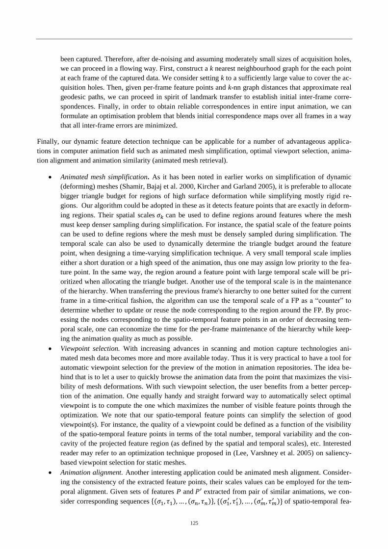
125

been captured. Therefore, after de-noising and assuming moderately small sizes of acquisition holes,

we can proceed in a flowing way. First, construct a k nearest neighbourhood graph for the each point

at each frame of the captured data. We consider setting k to a sufficiently large value to cover the ac-

quisition holes. Then, given per-frame feature points and k-nn graph distances that approximate real

geodesic paths, we can proceed in spirit of landmark transfer to establish initial inter-frame corre-

spondences. Finally, in order to obtain reliable correspondences in entire input animation, we can

formulate an optimisation problem that blends initial correspondence maps over all frames in a way

that all inter-frame errors are minimized.

Finally, our dynamic feature detection technique can be applicable for a number of advantageous applica-

tions in computer animation field such as animated mesh simplification, optimal viewport selection, anima-

tion alignment and animation similarity (animated mesh retrieval).

Animated mesh simplification. As it has been noted in earlier works on simplification of dynamic

(deforming) meshes (Shamir, Bajaj et al. 2000, Kircher and Garland 2005), it is preferable to allocate

bigger triangle budget for regions of high surface deformation while simplifying mostly rigid re-

gions. Our algorithm could be adopted in these as it detects feature points that are exactly in deform-

ing regions. Their spatial scales can be used to define regions around features where the mesh

must keep denser sampling during simplification. For instance, the spatial scale of the feature points

can be used to define regions where the mesh must be densely sampled during simplification. The

temporal scale can also be used to dynamically determine the triangle budget around the feature

point, when designing a time-varying simplification technique. A very small temporal scale implies

either a short duration or a high speed of the animation, thus one may assign low priority to the fea-

ture point. In the same way, the region around a feature point with large temporal scale will be pri-

oritized when allocating the triangle budget. Another use of the temporal scale is in the maintenance

of the hierarchy. When transferring the previous frame's hierarchy to one better suited for the current

frame in a time-critical fashion, the algorithm can use the temporal scale of a FP as a “counter” to

determine whether to update or reuse the node corresponding to the region around the FP. By proc-

essing the nodes corresponding to the spatio-temporal feature points in an order of decreasing tem-

poral scale, one can economize the time for the per-frame maintenance of the hierarchy while keep-

ing the animation quality as much as possible.

Viewpoint selection. With increasing advances in scanning and motion capture technologies ani-

mated mesh data becomes more and more available today. Thus it is very practical to have a tool for

automatic viewpoint selection for the preview of the motion in animation repositories. The idea be-

hind that is to let a user to quickly browse the animation data from the point that maximizes the visi-

bility of mesh deformations. With such viewpoint selection, the user benefits from a better percep-

tion of the animation. One equally handy and straight forward way to automatically select optimal

viewpoint is to compute the one which maximizes the number of visible feature points through the

optimization. We note that our spatio-temporal feature points can simplify the selection of good

viewpoint(s). For instance, the quality of a viewpoint could be defined as a function of the visibility

of the spatio-temporal feature points in terms of the total number, temporal variability and the con-

cavity of the projected feature region (as defined by the spatial and temporal scales), etc. Interested

reader may refer to an optimization technique proposed in (Lee, Varshney et al. 2005) on saliency-

based viewpoint selection for static meshes.

Animation alignment. Another interesting application could be animated mesh alignment. Consider-

ing the consistency of the extracted feature points, their scales values can be employed for the tem-

poral alignment. Given sets of features P and extracted from pair of similar animations, we con-

sider corresponding sequences

of spatio-temporal fea-

126

ture scales aligned along the time they were detected. Existing algorithms of sequence alignment

such as (Gotoh 1990) can then be used to compute the temporal alignment between them. In addition

to the spatial- and temporal- scales, more sophisticated feature descriptors can also be used to com-

pose the sequences.

Animation similarity. We can also think of extending the above mentioned animation alignment al-

gorithm towards a measurement of animation similarity. From the feature sequence alignment map,

we can sum up all penalty gaps i.e. some predefined costs for all features for which no match can be

found. That cost function could serve as a distance metric between the animations and hence be a

measure of dissimilarity/similarity. Note that an important by-product of the animation similarity is

the animated mesh retrieval, which is particularly beneficial in emerging dynamic data repositories.

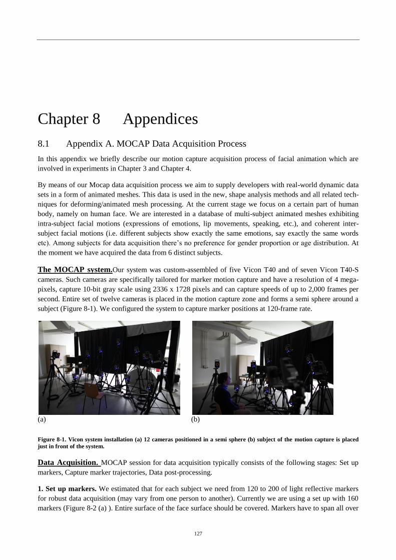
127

Chapter 8 Appendices

8.1 Appendix A. MOCAP Data Acquisition Process

In this appendix we briefly describe our motion capture acquisition process of facial animation which are

involved in experiments in Chapter 3 and Chapter 4.

By means of our Mocap data acquisition process we aim to supply developers with real-world dynamic data

sets in a form of animated meshes. This data is used in the new, shape analysis methods and all related tech-

niques for deforming/animated mesh processing. At the current stage we focus on a certain part of human

body, namely on human face. We are interested in a database of multi-subject animated meshes exhibiting

intra-subject facial motions (expressions of emotions, lip movements, speaking, etc.), and coherent inter-

subject facial motions (i.e. different subjects show exactly the same emotions, say exactly the same words

etc). Among subjects for data acquisition there’s no preference for gender proportion or age distribution. At

the moment we have acquired the data from 6 distinct subjects.

The MOCAP system.Our system was custom-assembled of five Vicon T40 and of seven Vicon T40-S

cameras. Such cameras are specifically tailored for marker motion capture and have a resolution of 4 mega-

pixels, capture 10-bit gray scale using 2336 x 1728 pixels and can capture speeds of up to 2,000 frames per

second. Entire set of twelve cameras is placed in the motion capture zone and forms a semi sphere around a

subject (Figure 8-1). We configured the system to capture marker positions at 120-frame rate.

(a) (b)

Figure 8-1. Vicon system installation (a) 12 cameras positioned in a semi sphere (b) subject of the motion capture is placed

just in front of the system.

Data Acquisition. MOCAP session for data acquisition typically consists of the following stages: Set up

markers, Capture marker trajectories, Data post-processing.

1. Set up markers. We estimated that for each subject we need from 120 to 200 of light reflective markers

for robust data acquisition (may vary from one person to another). Currently we are using a set up with 160

markers (Figure 8-2 (a) ). Entire surface of the face surface should be covered. Markers have to span all over

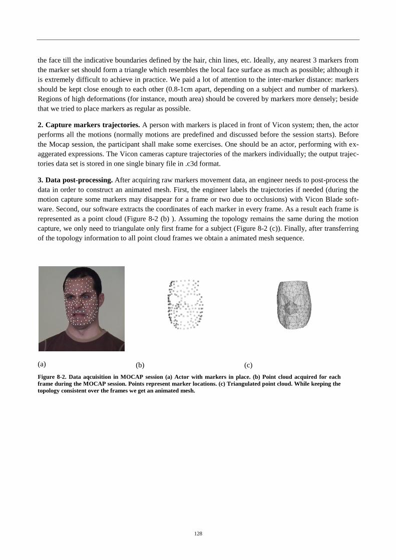
128

the face till the indicative boundaries defined by the hair, chin lines, etc. Ideally, any nearest 3 markers from

the marker set should form a triangle which resembles the local face surface as much as possible; although it

is extremely difficult to achieve in practice. We paid a lot of attention to the inter-marker distance: markers

should be kept close enough to each other (0.8-1cm apart, depending on a subject and number of markers).

Regions of high deformations (for instance, mouth area) should be covered by markers more densely; beside

that we tried to place markers as regular as possible.

2. Capture markers trajectories. A person with markers is placed in front of Vicon system; then, the actor

performs all the motions (normally motions are predefined and discussed before the session starts). Before

the Mocap session, the participant shall make some exercises. One should be an actor, performing with ex-

aggerated expressions. The Vicon cameras capture trajectories of the markers individually; the output trajec-

tories data set is stored in one single binary file in .c3d format.

3. Data post-processing. After acquiring raw markers movement data, an engineer needs to post-process the

data in order to construct an animated mesh. First, the engineer labels the trajectories if needed (during the

motion capture some markers may disappear for a frame or two due to occlusions) with Vicon Blade soft-

ware. Second, our software extracts the coordinates of each marker in every frame. As a result each frame is

represented as a point cloud (Figure 8-2 (b) ). Assuming the topology remains the same during the motion

capture, we only need to triangulate only first frame for a subject (Figure 8-2 (c)). Finally, after transferring

of the topology information to all point cloud frames we obtain a animated mesh sequence.

(a)

(b)

(c)

Figure 8-2. Data aqcuisition in MOCAP session (a) Actor with markers in place. (b) Point cloud acquired for each

frame during the MOCAP session. Points represent marker locations. (c) Triangulated point cloud. While keeping the

topology consistent over the frames we get an animated mesh.

129

8.2 Appendix B : Subgraph matching using Ullmann's Algorithm

Our subgraph matching method in Chapter 5 is similar in spirit to Ullmann’s algorithm (Ullmann 1976). In

the literature the subgraph matching problem is often called subgraph isomorphism. Given the source and

target graphs, isomorphism is simply defined as a pair of injective mappings between vertices

and edges of and . In Ullmann's algorithm subgraph matching is determined by a tree-search enumera-

tion (Ullmann 1976), i.e. by systematic generation of all possible matches between and . Consider the

source and the target graphs , , , where and are node

labels, and are weighted matrices of adjacency. A subgraph matching can be formally represented as a

permutation matrix , . If the value of is equal to 1, it

means that th vertex of is mapped to th vertex of . Two sequential left-multiplications of by ,

modify the target's graph adjacency matrix accordingly to the permutation matrix, in other words,

the target's vertices are permutated according to . Given , permutation matrix defines a

subgraph isomorphism of to , if .

The valid permutation M has a following set of properties:

binary: contains only 0 and 1;

injection: exactly one 1 in each row, and not more than one 1 in each column;

In order to support partial matches (i.e. only a subset of the source’s vertices is mapped on the target) we

modify the property set by removing the injection property and substituting it with a weaker condition: not

more than one 1 in each row and column.

We use an iterative approach to find a permutation which corresponds to valid subgraph matching. First,

we initialize the permutation with all ones (all permutations are possible). Then, we prevent the mapping

of the source vertex to the target vertex which has a smaller degree:

where denotes a degree of a vertex.

When the initialization is done, we generate systematically all valid permutation matrices by means of a

depth-first tree search. is located in the root of a search tree; the tree node at level is binded with a par-

tial permutation matrix, which maps precisely first vertices from to . For each next we select a

matching for (l + 1)th vertex from the source and check whether the weights of the new matching pair of

nodes are consistent. If corresponding weights are within a user-defined error threshold, we continue going

down the search tree. If the weight constraints are violated, we prune the search branch and come back to the

parent search node. When the generation of permutations is done, as an output { we have a set of

valid isomorphisms and a set of partial isomorphisms between and ; or in case when there is no valid

isomorphism, the output is an empty set .

130

References

Aiger, D., et al. (2008). 4-points congruent sets for robust pairwise surface registration. ACM Transactions

on Graphics (TOG), ACM.

Allen, B., Curless, B., & Popović, Z. (2002, July). Articulated body deformation from range scan data.

In ACM Transactions on Graphics (TOG) (Vol. 21, No. 3, pp. 612-619). ACM.

Allen, B., Curless, B., & Popović, Z. (2003, July). The space of human body shapes: reconstruction and

parameterization from range scans. In ACM Transactions on Graphics (TOG) (Vol. 22, No. 3, pp. 587-

594). ACM.

Allen, B., Curless, B., Popović, Z., & Hertzmann, A. (2006, September). Learning a correlated model of

identity and pose-dependent body shape variation for real-time synthesis. In Proceedings of the 2006

ACM SIGGRAPH/Eurographics symposium on Computer animation (pp. 147-156). Eurographics

Association.

Anguelov, D., et al. (2005). "The correlated correspondence algorithm for unsupervised registration of

nonrigid surfaces." Advances in neural information processing systems 17: 33-40.

Arcila, R., et al. (2010). "A framework for motion-based mesh sequence segmentation."

Arcila, R., et al. (2013). "Segmentation of temporal mesh sequences into rigidly moving components."

Graphical Models 75(1): 10-22.

Kin‐Chung Au, O., Tai, C. L., Cohen‐Or, D., Zheng, Y., & Fu, H. (2010, May). Electors voting for fast

automatic shape correspondence. In Computer Graphics Forum (Vol. 29, No. 2, pp. 645-654). Blackwell

Publishing Ltd.

Autodesk, I. "Autodesk Maya." from http://www.autodesk.com/products/maya/overview.

Bartolini, G. (2006). "On Poicarés Uniformization Theorem."

Bay, H., et al. (2006). Surf: Speeded up robust features. Computer Vision–ECCV 2006, Springer: 404-417.

Belongie, S., et al. (2000). Shape context: A new descriptor for shape matching and object recognition.

NIPS.

Bertsekas, D. P. (1999). Nonlinear programming.

Besl, P. J., & McKay, N. D. (1992, April). Method for registration of 3-D shapes. In Robotics-DL

tentative (pp. 586-606). International Society for Optics and Photonics.

Biasotti, S., Marini, S., Spagnuolo, M., & Falcidieno, B. (2006). Sub-part correspondence by structural

descriptors of 3D shapes. Computer-Aided Design, 38(9), 1002-1019.

Blanz, V., & Vetter, T. (1999, July). A morphable model for the synthesis of 3D faces. In Proceedings of the

26th annual conference on Computer graphics and interactive techniques (pp. 187-194). ACM

Press/Addison-Wesley Publishing Co..

Borg, I., & Groenen, P. J. (2005). Modern multidimensional scaling: Theory and applications. Springer

Science & Business Media.

Boykov, Y., Veksler, O., & Zabih, R. (2001). Fast approximate energy minimization via graph cuts. Pattern

Analysis and Machine Intelligence, IEEE Transactions on, 23(11), 1222-1239.

Bronstein, A. M., Bronstein, M. M., & Kimmel, R. (2006). Generalized multidimensional scaling: a

framework for isometry-invariant partial surface matching. Proceedings of the National Academy of

Sciences of the United States of America, 103(5), 1168-1172.

Bronstein, A. M., Bronstein, M. M., Kimmel, R., Mahmoudi, M., & Sapiro, G. (2010). A Gromov-Hausdorff

framework with diffusion geometry for topologically-robust non-rigid shape matching. International

Journal of Computer Vision, 89(2-3), 266-286.

Bronstein, M. M. and I. Kokkinos (2010). Scale-invariant heat kernel signatures for non-rigid shape

recognition. Computer Vision and Pattern Recognition (CVPR), 2010 IEEE Conference on, IEEE.

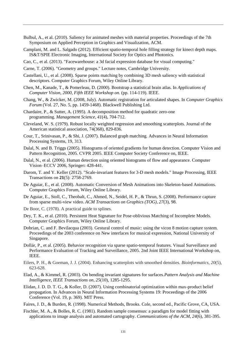
131

Bulbul, A., et al. (2010). Saliency for animated meshes with material properties. Proceedings of the 7th

Symposium on Applied Perception in Graphics and Visualization, ACM.

Camplani, M. and L. Salgado (2012). Efficient spatio-temporal hole filling strategy for kinect depth maps.

IS&T/SPIE Electronic Imaging, International Society for Optics and Photonics.

Cao, C., et al. (2013). "Facewarehouse: a 3d facial expression database for visual computing."

Carne, T. (2006). "Geometry and groups." Lecture notes, Cambridge University.

Castellani, U., et al. (2008). Sparse points matching by combining 3D mesh saliency with statistical

descriptors. Computer Graphics Forum, Wiley Online Library.

Chen, M., Kanade, T., & Pomerleau, D. (2000). Bootstrap a statistical brain atlas. In Applications of

Computer Vision, 2000, Fifth IEEE Workshop on. (pp. 114-119). IEEE.

Chang, W., & Zwicker, M. (2008, July). Automatic registration for articulated shapes. In Computer Graphics

Forum (Vol. 27, No. 5, pp. 1459-1468). Blackwell Publishing Ltd.

Chardaire, P., & Sutter, A. (1995). A decomposition method for quadratic zero-one

programming. Management Science, 41(4), 704-712.

Cleveland, W. S. (1979). Robust locally weighted regression and smoothing scatterplots. Journal of the

American statistical association, 74(368), 829-836.

Cour, T., Srinivasan, P., & Shi, J. (2007). Balanced graph matching. Advances in Neural Information

Processing Systems, 19, 313.

Dalal, N. and B. Triggs (2005). Histograms of oriented gradients for human detection. Computer Vision and

Pattern Recognition, 2005. CVPR 2005. IEEE Computer Society Conference on, IEEE.

Dalal, N., et al. (2006). Human detection using oriented histograms of flow and appearance. Computer

Vision–ECCV 2006, Springer: 428-441.

Darom, T. and Y. Keller (2012). "Scale-invariant features for 3-D mesh models." Image Processing, IEEE

Transactions on 21(5): 2758-2769.

De Aguiar, E., et al. (2008). Automatic Conversion of Mesh Animations into Skeleton‐based Animations.

Computer Graphics Forum, Wiley Online Library.

De Aguiar, E., Stoll, C., Theobalt, C., Ahmed, N., Seidel, H. P., & Thrun, S. (2008). Performance capture

from sparse multi-view video. ACM Transactions on Graphics (TOG), 27(3), 98.

De Boor, C. (1978). A practical guide to splines.

Dey, T. K., et al. (2010). Persistent Heat Signature for Pose‐oblivious Matching of Incomplete Models.

Computer Graphics Forum, Wiley Online Library.

Dobrian, C. and F. Bevilacqua (2003). Gestural control of music: using the vicon 8 motion capture system.

Proceedings of the 2003 conference on New interfaces for musical expression, National University of

Singapore.

Dollár, P., et al. (2005). Behavior recognition via sparse spatio-temporal features. Visual Surveillance and

Performance Evaluation of Tracking and Surveillance, 2005. 2nd Joint IEEE International Workshop on,

IEEE.

Eilers, P. H., & Goeman, J. J. (2004). Enhancing scatterplots with smoothed densities. Bioinformatics, 20(5),

623-628.

Elad, A., & Kimmel, R. (2003). On bending invariant signatures for surfaces.Pattern Analysis and Machine

Intelligence, IEEE Transactions on, 25(10), 1285-1295.

Elidan, J. D. D. T. G., & Koller, D. (2007). Using combinatorial optimization within max-product belief

propagation. In Advances in Neural Information Processing Systems 19: Proceedings of the 2006

Conference (Vol. 19, p. 369). MIT Press.

Faires, J. D., & Burden, R. (1998). Numerical Methods, Brooks. Cole, second ed., Pacific Grove, CA, USA.

Fischler, M. A., & Bolles, R. C. (1981). Random sample consensus: a paradigm for model fitting with

applications to image analysis and automated cartography. Communications of the ACM, 24(6), 381-395.

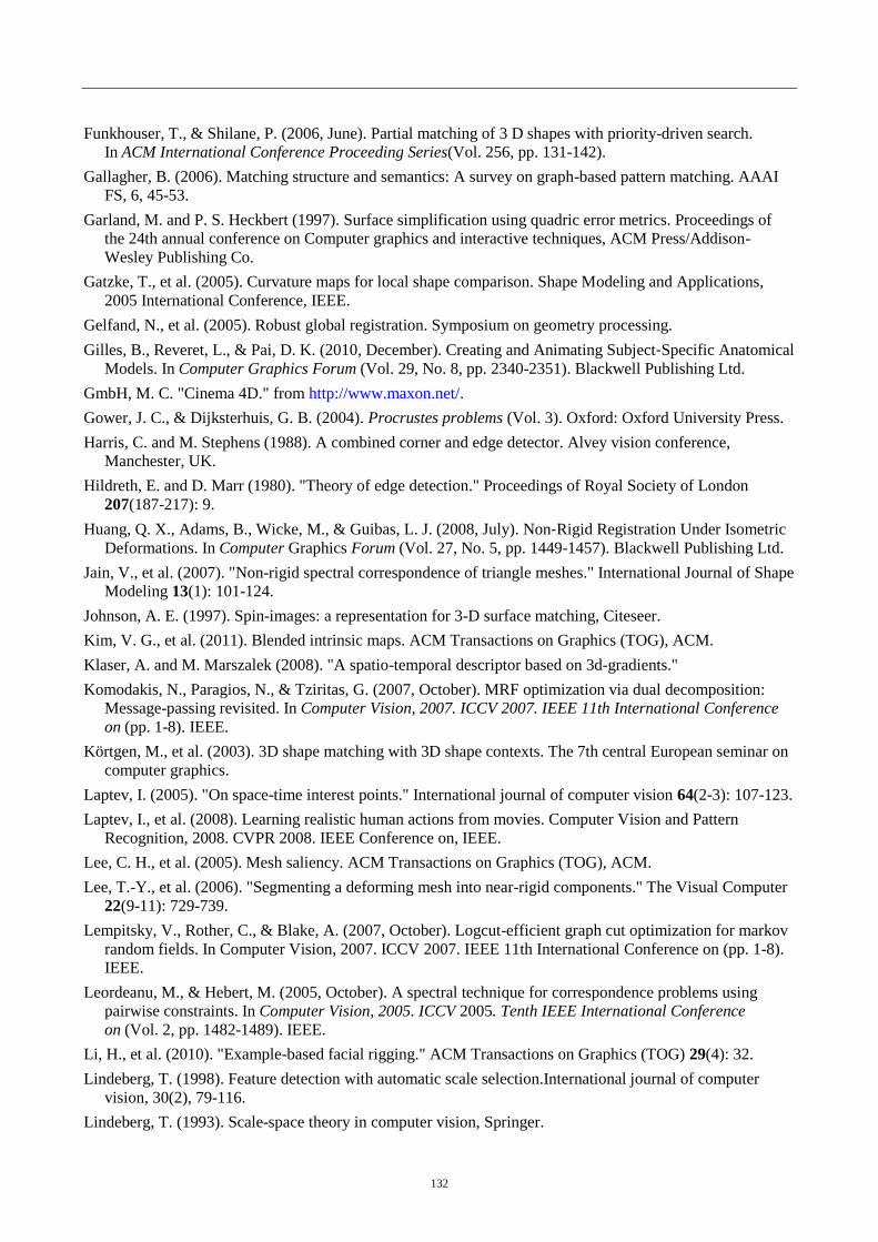
132

Funkhouser, T., & Shilane, P. (2006, June). Partial matching of 3 D shapes with priority-driven search.

In ACM International Conference Proceeding Series(Vol. 256, pp. 131-142).

Gallagher, B. (2006). Matching structure and semantics: A survey on graph-based pattern matching. AAAI

FS, 6, 45-53.

Garland, M. and P. S. Heckbert (1997). Surface simplification using quadric error metrics. Proceedings of

the 24th annual conference on Computer graphics and interactive techniques, ACM Press/Addison-

Wesley Publishing Co.

Gatzke, T., et al. (2005). Curvature maps for local shape comparison. Shape Modeling and Applications,

2005 International Conference, IEEE.

Gelfand, N., et al. (2005). Robust global registration. Symposium on geometry processing.

Gilles, B., Reveret, L., & Pai, D. K. (2010, December). Creating and Animating Subject‐Specific Anatomical

Models. In Computer Graphics Forum (Vol. 29, No. 8, pp. 2340-2351). Blackwell Publishing Ltd.

GmbH, M. C. "Cinema 4D." from http://www.maxon.net/.

Gower, J. C., & Dijksterhuis, G. B. (2004). Procrustes problems (Vol. 3). Oxford: Oxford University Press.

Harris, C. and M. Stephens (1988). A combined corner and edge detector. Alvey vision conference,

Manchester, UK.

Hildreth, E. and D. Marr (1980). "Theory of edge detection." Proceedings of Royal Society of London

207(187-217): 9.

Huang, Q. X., Adams, B., Wicke, M., & Guibas, L. J. (2008, July). Non‐Rigid Registration Under Isometric

Deformations. In Computer Graphics Forum (Vol. 27, No. 5, pp. 1449-1457). Blackwell Publishing Ltd.

Jain, V., et al. (2007). "Non-rigid spectral correspondence of triangle meshes." International Journal of Shape

Modeling 13(1): 101-124.

Johnson, A. E. (1997). Spin-images: a representation for 3-D surface matching, Citeseer.

Kim, V. G., et al. (2011). Blended intrinsic maps. ACM Transactions on Graphics (TOG), ACM.

Klaser, A. and M. Marszalek (2008). "A spatio-temporal descriptor based on 3d-gradients."

Komodakis, N., Paragios, N., & Tziritas, G. (2007, October). MRF optimization via dual decomposition:

Message-passing revisited. In Computer Vision, 2007. ICCV 2007. IEEE 11th International Conference

on (pp. 1-8). IEEE.

Körtgen, M., et al. (2003). 3D shape matching with 3D shape contexts. The 7th central European seminar on

computer graphics.

Laptev, I. (2005). "On space-time interest points." International journal of computer vision 64(2-3): 107-123.

Laptev, I., et al. (2008). Learning realistic human actions from movies. Computer Vision and Pattern

Recognition, 2008. CVPR 2008. IEEE Conference on, IEEE.

Lee, C. H., et al. (2005). Mesh saliency. ACM Transactions on Graphics (TOG), ACM.

Lee, T.-Y., et al. (2006). "Segmenting a deforming mesh into near-rigid components." The Visual Computer

22(9-11): 729-739.

Lempitsky, V., Rother, C., & Blake, A. (2007, October). Logcut-efficient graph cut optimization for markov

random fields. In Computer Vision, 2007. ICCV 2007. IEEE 11th International Conference on (pp. 1-8).

IEEE.

Leordeanu, M., & Hebert, M. (2005, October). A spectral technique for correspondence problems using

pairwise constraints. In Computer Vision, 2005. ICCV 2005. Tenth IEEE International Conference

on (Vol. 2, pp. 1482-1489). IEEE.

Li, H., et al. (2010). "Example-based facial rigging." ACM Transactions on Graphics (TOG) 29(4): 32.

Lindeberg, T. (1998). Feature detection with automatic scale selection.International journal of computer

vision, 30(2), 79-116.

Lindeberg, T. (1993). Scale-space theory in computer vision, Springer.

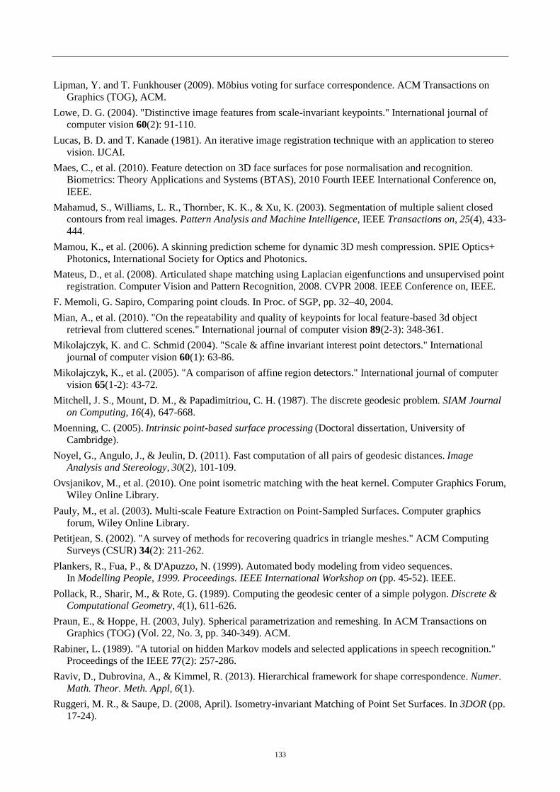
133

Lipman, Y. and T. Funkhouser (2009). Möbius voting for surface correspondence. ACM Transactions on

Graphics (TOG), ACM.

Lowe, D. G. (2004). "Distinctive image features from scale-invariant keypoints." International journal of

computer vision 60(2): 91-110.

Lucas, B. D. and T. Kanade (1981). An iterative image registration technique with an application to stereo

vision. IJCAI.

Maes, C., et al. (2010). Feature detection on 3D face surfaces for pose normalisation and recognition.

Biometrics: Theory Applications and Systems (BTAS), 2010 Fourth IEEE International Conference on,

IEEE.

Mahamud, S., Williams, L. R., Thornber, K. K., & Xu, K. (2003). Segmentation of multiple salient closed

contours from real images. Pattern Analysis and Machine Intelligence, IEEE Transactions on, 25(4), 433-

444.

Mamou, K., et al. (2006). A skinning prediction scheme for dynamic 3D mesh compression. SPIE Optics+

Photonics, International Society for Optics and Photonics.

Mateus, D., et al. (2008). Articulated shape matching using Laplacian eigenfunctions and unsupervised point

registration. Computer Vision and Pattern Recognition, 2008. CVPR 2008. IEEE Conference on, IEEE.

F. Memoli, G. Sapiro, Comparing point clouds. In Proc. of SGP, pp. 32–40, 2004.

Mian, A., et al. (2010). "On the repeatability and quality of keypoints for local feature-based 3d object

retrieval from cluttered scenes." International journal of computer vision 89(2-3): 348-361.

Mikolajczyk, K. and C. Schmid (2004). "Scale & affine invariant interest point detectors." International

journal of computer vision 60(1): 63-86.

Mikolajczyk, K., et al. (2005). "A comparison of affine region detectors." International journal of computer

vision 65(1-2): 43-72.

Mitchell, J. S., Mount, D. M., & Papadimitriou, C. H. (1987). The discrete geodesic problem. SIAM Journal

on Computing, 16(4), 647-668.

Moenning, C. (2005). Intrinsic point-based surface processing (Doctoral dissertation, University of

Cambridge).

Noyel, G., Angulo, J., & Jeulin, D. (2011). Fast computation of all pairs of geodesic distances. Image

Analysis and Stereology, 30(2), 101-109.

Ovsjanikov, M., et al. (2010). One point isometric matching with the heat kernel. Computer Graphics Forum,

Wiley Online Library.

Pauly, M., et al. (2003). Multi‐scale Feature Extraction on Point‐Sampled Surfaces. Computer graphics

forum, Wiley Online Library.

Petitjean, S. (2002). "A survey of methods for recovering quadrics in triangle meshes." ACM Computing

Surveys (CSUR) 34(2): 211-262.

Plankers, R., Fua, P., & D'Apuzzo, N. (1999). Automated body modeling from video sequences.

In Modelling People, 1999. Proceedings. IEEE International Workshop on (pp. 45-52). IEEE.

Pollack, R., Sharir, M., & Rote, G. (1989). Computing the geodesic center of a simple polygon. Discrete &

Computational Geometry, 4(1), 611-626.

Praun, E., & Hoppe, H. (2003, July). Spherical parametrization and remeshing. In ACM Transactions on

Graphics (TOG) (Vol. 22, No. 3, pp. 340-349). ACM.

Rabiner, L. (1989). "A tutorial on hidden Markov models and selected applications in speech recognition."

Proceedings of the IEEE 77(2): 257-286.

Raviv, D., Dubrovina, A., & Kimmel, R. (2013). Hierarchical framework for shape correspondence. Numer.

Math. Theor. Meth. Appl, 6(1).

Ruggeri, M. R., & Saupe, D. (2008, April). Isometry-invariant Matching of Point Set Surfaces. In 3DOR (pp.

17-24).

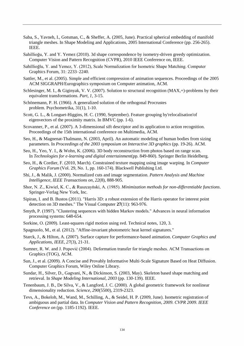
134

Saba, S., Yavneh, I., Gotsman, C., & Sheffer, A. (2005, June). Practical spherical embedding of manifold

triangle meshes. In Shape Modeling and Applications, 2005 International Conference (pp. 256-265).

IEEE.

Sahillioğu, Y. and Y. Yemez (2010). 3d shape correspondence by isometry-driven greedy optimization.

Computer Vision and Pattern Recognition (CVPR), 2010 IEEE Conference on, IEEE.

Sahillioğlu, . and emez, . (2012), Scale Normalization for Isometric Shape Matching. Computer

Graphics Forum, 31: 2233–2240.

Sattler, M., et al. (2005). Simple and efficient compression of animation sequences. Proceedings of the 2005

ACM SIGGRAPH/Eurographics symposium on Computer animation, ACM.

Schlesinger, M. I., & Giginyak, V. V. (2007). Solution to structural recognition (MAX,+)-problems by their

equivalent transformations. Part, 1, 3-15.

Schönemann, P. H. (1966). A generalized solution of the orthogonal Procrustes

problem. Psychometrika, 31(1), 1-10.

Scott, G. L., & Longuet-Higgins, H. C. (1990, September). Feature grouping by'relocalisation'of

eigenvectors of the proximity matrix. In BMVC (pp. 1-6).

Scovanner, P., et al. (2007). A 3-dimensional sift descriptor and its application to action recognition.

Proceedings of the 15th international conference on Multimedia, ACM.

Seo, H., & Magnenat-Thalmann, N. (2003, April). An automatic modeling of human bodies from sizing

parameters. In Proceedings of the 2003 symposium on Interactive 3D graphics (pp. 19-26). ACM.

Seo, H., Yeo, Y. I., & Wohn, K. (2006). 3D body reconstruction from photos based on range scan.

In Technologies for e-learning and digital entertainment(pp. 849-860). Springer Berlin Heidelberg.

Seo, H., & Cordier, F. (2010, March). Constrained texture mapping using image warping. In Computer

Graphics Forum (Vol. 29, No. 1, pp. 160-174). Blackwell Publishing Ltd.

Shi, J., & Malik, J. (2000). Normalized cuts and image segmentation. Pattern Analysis and Machine

Intelligence, IEEE Transactions on, 22(8), 888-905.

Shor, N. Z., Kiwiel, K. C., & Ruszcayǹski, A. (1985). Minimization methods for non-differentiable functions.

Springer-Verlag New York, Inc.

Sipiran, I. and B. Bustos (2011). "Harris 3D: a robust extension of the Harris operator for interest point

detection on 3D meshes." The Visual Computer 27(11): 963-976.

Smyth, P. (1997). "Clustering sequences with hidden Markov models." Advances in neural information

processing systems: 648-654.

Sorkine, O. (2009). Least-squares rigid motion using svd. Technical notes, 120, 3.

Spagnuolo, M., et al. (2012). "Affine-invariant photometric heat kernel signatures."

Starck, J., & Hilton, A. (2007). Surface capture for performance-based animation. Computer Graphics and

Applications, IEEE, 27(3), 21-31.

Sumner, R. W. and J. Popović (2004). Deformation transfer for triangle meshes. ACM Transactions on

Graphics (TOG), ACM.

Sun, J., et al. (2009). A Concise and Provably Informative Multi‐Scale Signature Based on Heat Diffusion.

Computer Graphics Forum, Wiley Online Library.

Sundar, H., Silver, D., Gagvani, N., & Dickinson, S. (2003, May). Skeleton based shape matching and

retrieval. In Shape Modeling International, 2003 (pp. 130-139). IEEE.

Tenenbaum, J. B., De Silva, V., & Langford, J. C. (2000). A global geometric framework for nonlinear

dimensionality reduction. Science, 290(5500), 2319-2323.

Tevs, A., Bokeloh, M., Wand, M., Schilling, A., & Seidel, H. P. (2009, June). Isometric registration of

ambiguous and partial data. In Computer Vision and Pattern Recognition, 2009. CVPR 2009. IEEE

Conference on (pp. 1185-1192). IEEE.

135

Tevs, Berner et al. (2011). Intrinsic shape matching by planned landmark sampling. Computer Graphics

Forum, Wiley Online Library.

Tierny, J., Vandeborre, J. P., & Daoudi, M. (2009, March). Partial 3D shape retrieval by reeb pattern

unfolding. In Computer Graphics Forum (Vol. 28, No. 1, pp. 41-55). Blackwell Publishing Ltd.

Torr, P. H., & Zisserman, A. (2000). MLESAC: A new robust estimator with application to estimating image

geometry. Computer Vision and Image Understanding, 78(1), 138-156.

Torresani, L., Kolmogorov, V., & Rother, C. (2008). Feature correspondence via graph matching: Models

and global optimization. In Computer Vision–ECCV 2008 (pp. 596-609). Springer Berlin Heidelberg.

Torresani, L., Kolmogorov, V., & Rother, C. (2013). A dual decomposition approach to feature

correspondence. Pattern Analysis and Machine Intelligence, IEEE Transactions on, 35(2), 259-271.

Tung, T., & Matsuyama, T. (2013). Invariant surface-based shape descriptor for dynamic surface encoding.

In Computer Vision–ACCV 2012 (pp. 486-499). Springer Berlin Heidelberg.

Tuytelaars, T., & Mikolajczyk, K. (2008). Local invariant feature detectors: a survey. Foundations and

Trends® in Computer Graphics and Vision, 3(3), 177-280.

Tuzel, O., Subbarao, R., & Meer, P. (2005, October). Simultaneous multiple 3D motion estimation via mode

finding on Lie groups. In Computer Vision, 2005. ICCV 2005. Tenth IEEE International Conference

on (Vol. 1, pp. 18-25). IEEE.

Ullmann, J. R. (1976). An algorithm for subgraph isomorphism. Journal of the ACM (JACM), 23(1), 31-42.

Valgaerts, L., et al. (2012). "Lightweight binocular facial performance capture under uncontrolled lighting."

ACM Trans. Graph. 31(6): 187.

Vlasic, D., Brand, M., Pfister, H., & Popović, J. (2005, July). Face transfer with multilinear models. In ACM

Transactions on Graphics (TOG) (Vol. 24, No. 3, pp. 426-433). ACM.

Vlasic, D., et al. (2007). Practical motion capture in everyday surroundings. ACM Transactions on Graphics

(TOG), ACM.

Wang, C., Bronstein, M. M., Bronstein, A. M., & Paragios, N. (2012). Discrete minimum distortion

correspondence problems for non-rigid shape matching. InScale Space and Variational Methods in

Computer Vision (pp. 580-591). Springer Berlin Heidelberg.

Webb, J. and J. Ashley (2012). Beginning Kinect Programming with the Microsoft Kinect SDK, Apress.

Weise, T., et al. (2011). "Realtime performance-based facial animation." ACM Transactions on Graphics

(TOG) 30(4): 77.

Weise, T., et al. (2009). Face/off: Live facial puppetry. Proceedings of the 2009 ACM

SIGGRAPH/Eurographics Symposium on Computer animation, ACM.

Tai, Y. W., & Park, I. K. (2014). Accurate and real-time depth video acquisition using Kinect–stereo camera

fusion. Optical Engineering, 53(4), 043110-043110.

Willems, G., et al. (2008). An efficient dense and scale-invariant spatio-temporal interest point detector.

Computer Vision–ECCV 2008, Springer: 650-663.

Zaharescu, A., et al. (2009). Surface feature detection and description with applications to mesh matching.

Computer Vision and Pattern Recognition, 2009. CVPR 2009. IEEE Conference on, IEEE.

Zelinka, S. and M. Garland (2004). Similarity-based surface modelling using geodesic fans. Proceedings of

the 2004 Eurographics/ACM SIGGRAPH symposium on Geometry processing, ACM.

Zhang, H., Sheffer, A., Cohen‐Or, D., Zhou, Q., Van Kaick, O., & Tagliasacchi, A. (2008, July).

Deformation‐Driven Shape Correspondence. In Computer Graphics Forum (Vol. 27, No. 5, pp. 1431-

1439). Blackwell Publishing Ltd.

Zhang, Z. (2000). A flexible new technique for camera calibration. Pattern Analysis and Machine

Intelligence, IEEE Transactions on, 22(11), 1330-1334.

136

Zhu, C., Byrd, R. H., Lu, P., & Nocedal, J. (1997). Algorithm 778: L-BFGS-B: Fortran subroutines for large-

scale bound-constrained optimization. ACM Transactions on Mathematical Software (TOMS), 23(4), 550-

560.