
core.ac.uk · %NVUEDEL OBTENTIONDU %0$503"5 %&- 6/*7&34*5² %& 506-064& $ÏLIVRÏPAR...
217
M : Institut National Polytechnique de Toulouse (INP Toulouse) Mécanique, Energétique, Génie civil et Procédés (MEGeP) Mechanisms affecting the dynamic response of swirled flames in gas turbines vendredi 28 septembre 2012 Sebastian HERMETH Dynamique des fluides Prof. Sebastian DUCRUIX, Ecole Centrale Paris Prof. Jim KOK, University of Twente Laurent GICQUEL Gabriel STAFFELBACH CERFACS Prof. Matthew JUNIPER, University of Cambrigde, Président Prof. Wolfgang POLIFKE, University TU Munich, Membre Prof. Thierry POINSOT, University of Toulouse, Membre Vyacheslav ANISIMOV, Ansaldo Energia S.p.A., Membre
Transcript of core.ac.uk · %NVUEDEL OBTENTIONDU %0$503"5 %&- 6/*7&34*5² %& 506-064& $ÏLIVRÏPAR...
M :
Institut National Polytechnique de Toulouse (INP Toulouse)
Mécanique, Energétique, Génie civil et Procédés (MEGeP)
Mechanisms affecting the dynamic response of swirled flamesin gas turbines
vendredi 28 septembre 2012Sebastian HERMETH
Dynamique des fluides
Prof. Sebastian DUCRUIX, Ecole Centrale ParisProf. Jim KOK, University of Twente
Laurent GICQUELGabriel STAFFELBACH
CERFACS
Prof. Matthew JUNIPER, University of Cambrigde, PrésidentProf. Wolfgang POLIFKE, University TU Munich, MembreProf. Thierry POINSOT, University of Toulouse, MembreVyacheslav ANISIMOV, Ansaldo Energia S.p.A., Membre

Mechanisms affecting the dynamic response of swirled flames ingas turbines
Abstract:Modern pollutant regulations have led to a trend towards lean combustion systemswhich are prone to thermo-acoustic instabilities. The ability of Large Eddy Sim-ulation (LES) to handle complex industrial heavy-duty gas turbines is evidencedduring this thesis work. First, LES is applied to an academic single burner in or-der to validate the modeling against measurements performed at TU Berlin andagainst OpenFoam LES simulations done at Siemens. The coupling between acous-tics and combustion is modeled with the Flame Transfer Function (FTF) approach,and swirl number fluctuations are identified changing the FTF amplitude responseof the flame.Then, an industrial gas turbine is analyzed for two different burner geometries andoperating conditions. The FTF is only slightly influenced for the two operatingpoints but slight modifications of the swirler geometry do modify the characteristicsof the FTF, showing that a simple model taking only into account the flight time isnot appropriate and additional mechanisms are at play. Those mechanisms are iden-tified being the inlet velocity, the swirl and the inlet mixture fraction fluctuations.The latter is caused by two mechanisms: 1) the pulsating injected fuel flow rateand 2) the fluctuating trajectory of the fuel jets. Although the diagonal swirler isdesigned to provide good mixing, effects of mixing heterogeneities at the combustionchamber inlet do occur. Mixture perturbations phase with velocity (and hence withswirl) fluctuations and combine with them to lead to different FTF results. AnotherFTF approach linking heat release rate to inlet velocity and mixture fraction fluc-tuation (MISO model) shows further to be a good solution for complex systems. Anonlinear analysis shows that the forcing amplitude not only leads to a saturation ofthe flame, but also to changes of the delay response. Flame saturation is only truefor the global FTF and the gain increases locally with increasing forcing amplitude.Both, the linear and the nonlinear flames, are not compact: flame regions locatedright next to each other exhibited significant differences in delay meaning that atthe same instant certain parts of the flame damp the excitation while others feed it.
Keywords: Combustion instabilities, Large Eddy Simulation, Gas turbine engines


Contents
I Introduction and context 1
1 Introduction 31.1 Energy consumption . . . . . . . . . . . . . . . . . . . . . . . . . . . 31.2 Combustion and environment . . . . . . . . . . . . . . . . . . . . . . 51.3 Gas turbines . . . . . . . . . . . . . . . . . . . . . . . . . . . . . . . 7
1.3.1 History . . . . . . . . . . . . . . . . . . . . . . . . . . . . . . 71.3.2 Operation theory . . . . . . . . . . . . . . . . . . . . . . . . . 8
1.4 Objectives and organization of the present work . . . . . . . . . . . . 101.4.1 Objectives . . . . . . . . . . . . . . . . . . . . . . . . . . . . . 101.4.2 Organization of this work . . . . . . . . . . . . . . . . . . . . 11
II Theoretical background 13
2 Thermo-acoustic instabilities 152.1 Causes of thermo-acoustic instabilities . . . . . . . . . . . . . . . . . 162.2 Control of thermo-acoustic instabilities . . . . . . . . . . . . . . . . . 192.3 Study of thermo-acoustic instabilities . . . . . . . . . . . . . . . . . . 20
2.3.1 Forced response method . . . . . . . . . . . . . . . . . . . . . 202.3.2 Self-excitation method . . . . . . . . . . . . . . . . . . . . . . 25
2.4 CFD as a tool to study thermo-acoustic instabilities . . . . . . . . . 26
3 Numerical method 293.1 Governing equations . . . . . . . . . . . . . . . . . . . . . . . . . . . 30
3.1.1 Equation of state . . . . . . . . . . . . . . . . . . . . . . . . . 303.1.2 Species transport . . . . . . . . . . . . . . . . . . . . . . . . . 313.1.3 Chemistry modeling . . . . . . . . . . . . . . . . . . . . . . . 31
3.2 Large-Eddy Simulation . . . . . . . . . . . . . . . . . . . . . . . . . . 323.2.1 Filtered Navier-Stokes equations . . . . . . . . . . . . . . . . 323.2.2 Sub-grid scale modeling . . . . . . . . . . . . . . . . . . . . . 343.2.3 Combustion modeling . . . . . . . . . . . . . . . . . . . . . . 35
3.3 Discretization . . . . . . . . . . . . . . . . . . . . . . . . . . . . . . . 363.3.1 Cell-vertex method . . . . . . . . . . . . . . . . . . . . . . . . 363.3.2 Time advancement . . . . . . . . . . . . . . . . . . . . . . . . 363.3.3 Convection scheme . . . . . . . . . . . . . . . . . . . . . . . . 36
3.4 Boundary conditions . . . . . . . . . . . . . . . . . . . . . . . . . . . 373.4.1 Inlet and outlet boundary conditions . . . . . . . . . . . . . . 373.4.2 Wall treatment . . . . . . . . . . . . . . . . . . . . . . . . . . 38
3.5 LES and System identification . . . . . . . . . . . . . . . . . . . . . . 393.5.1 Excitation signal . . . . . . . . . . . . . . . . . . . . . . . . . 39
vi Contents
3.5.2 System identification . . . . . . . . . . . . . . . . . . . . . . . 40
III Application to a perfectly premixed swirler combustor: theFVV burner 45
4 Target configuration 474.1 The FVV test rig . . . . . . . . . . . . . . . . . . . . . . . . . . . . . 47
4.1.1 Experimental set-up . . . . . . . . . . . . . . . . . . . . . . . 484.1.2 Operating point . . . . . . . . . . . . . . . . . . . . . . . . . . 49
4.2 Description of the numerical setup . . . . . . . . . . . . . . . . . . . 494.2.1 Computational mesh . . . . . . . . . . . . . . . . . . . . . . . 504.2.2 Boundary conditions . . . . . . . . . . . . . . . . . . . . . . . 514.2.3 Numerical parameters . . . . . . . . . . . . . . . . . . . . . . 51
5 LES of the reacting unforced and forced flows in the FVV setup 535.1 Reacting flow fields . . . . . . . . . . . . . . . . . . . . . . . . . . . . 53
5.1.1 Mean reacting flow fields with AVBP . . . . . . . . . . . . . . 535.1.2 Comparison Between AVBP, Openfoam and PIV . . . . . . . 56
5.2 Forced reacting flow . . . . . . . . . . . . . . . . . . . . . . . . . . . 605.2.1 Pulsation procedure . . . . . . . . . . . . . . . . . . . . . . . 605.2.2 Flame Transfer Function . . . . . . . . . . . . . . . . . . . . . 605.2.3 Mechanisms affecting the FTF . . . . . . . . . . . . . . . . . 61
5.3 Conclusions . . . . . . . . . . . . . . . . . . . . . . . . . . . . . . . . 63
IV Application to an industrial combustor: A Double SwirlerTechnically Premixed Burner 65
6 Target configuration 676.1 Geometries . . . . . . . . . . . . . . . . . . . . . . . . . . . . . . . . 67
6.1.1 Real gas turbine . . . . . . . . . . . . . . . . . . . . . . . . . 686.1.2 Experimental test rig for cold flow validation . . . . . . . . . 70
6.2 Description of the numerical setup . . . . . . . . . . . . . . . . . . . 716.2.1 Computational mesh . . . . . . . . . . . . . . . . . . . . . . . 716.2.2 Boundary conditions . . . . . . . . . . . . . . . . . . . . . . . 746.2.3 Numerical parameters . . . . . . . . . . . . . . . . . . . . . . 75
7 Numerical results for the unforced flame 797.1 Non-reacting flow fields . . . . . . . . . . . . . . . . . . . . . . . . . 79
7.1.1 Instantaneous flow characteristics . . . . . . . . . . . . . . . . 797.1.2 Mean flow fields . . . . . . . . . . . . . . . . . . . . . . . . . 807.1.3 Pressure drop . . . . . . . . . . . . . . . . . . . . . . . . . . . 837.1.4 Concluding remarks . . . . . . . . . . . . . . . . . . . . . . . 85
7.2 Reacting flow fields . . . . . . . . . . . . . . . . . . . . . . . . . . . . 87
Contents vii
7.2.1 Instantaneous flow characteristics . . . . . . . . . . . . . . . . 877.2.2 Mean flow field . . . . . . . . . . . . . . . . . . . . . . . . . . 877.2.3 Acoustic characteristics of the chamber . . . . . . . . . . . . . 967.2.4 Concluding remarks . . . . . . . . . . . . . . . . . . . . . . . 96
7.3 Flame stabilization . . . . . . . . . . . . . . . . . . . . . . . . . . . . 997.3.1 Concluding remarks . . . . . . . . . . . . . . . . . . . . . . . 100
7.4 Bi-stable behaviour of the reacting flow . . . . . . . . . . . . . . . . 1017.4.1 Concluding remarks . . . . . . . . . . . . . . . . . . . . . . . 106
7.5 Quality of the LES . . . . . . . . . . . . . . . . . . . . . . . . . . . . 107
8 Acoustically perturbed flame 1098.1 Pulsation procedure and system identification . . . . . . . . . . . . . 112
8.1.1 Pulsation procedure . . . . . . . . . . . . . . . . . . . . . . . 1128.1.2 System identification . . . . . . . . . . . . . . . . . . . . . . . 113
8.2 Flame Transfer Function . . . . . . . . . . . . . . . . . . . . . . . . . 1148.2.1 Comparison of the identification methods . . . . . . . . . . . 116
8.3 Influence of operating conditions and burner outlets . . . . . . . . . 1188.3.1 Mean pulsated flow fields . . . . . . . . . . . . . . . . . . . . 1188.3.2 Dynamic flame response . . . . . . . . . . . . . . . . . . . . . 1228.3.3 Local comparison of FTF . . . . . . . . . . . . . . . . . . . . 1228.3.4 Effect of mixture and swirl perturbation . . . . . . . . . . . . 1238.3.5 Concluding remarks . . . . . . . . . . . . . . . . . . . . . . . 126
8.4 Effects of forcing frequencies . . . . . . . . . . . . . . . . . . . . . . . 1298.4.1 Dynamic flame response . . . . . . . . . . . . . . . . . . . . . 1298.4.2 Local comparison of FTF . . . . . . . . . . . . . . . . . . . . 1298.4.3 Effects of fuel heterogeneities and swirl perturbation . . . . . 1328.4.4 Concluding remarks . . . . . . . . . . . . . . . . . . . . . . . 140
9 Identification of mechanisms controlling FTFs 1439.1 Effects of mass flow rate perturbation . . . . . . . . . . . . . . . . . 145
9.1.1 Mean reacting flow fields . . . . . . . . . . . . . . . . . . . . . 1459.1.2 Dynamics of the reacting flow fields . . . . . . . . . . . . . . . 1499.1.3 Concluding remarks . . . . . . . . . . . . . . . . . . . . . . . 150
9.2 Effects of mixture fluctuation . . . . . . . . . . . . . . . . . . . . . . 1529.2.1 Dynamic flame response . . . . . . . . . . . . . . . . . . . . . 1539.2.2 Propagation of mixing heterogeneities . . . . . . . . . . . . . 1549.2.3 Swirl number perturbation . . . . . . . . . . . . . . . . . . . . 1609.2.4 Concluding remarks . . . . . . . . . . . . . . . . . . . . . . . 160
9.3 Combined Flame Transfer Function approach . . . . . . . . . . . . . 161
10 Nonlinear analysis 16310.1 Mean pulsated flow fields . . . . . . . . . . . . . . . . . . . . . . . . 16510.2 Effect of pulsation amplitude on FDF . . . . . . . . . . . . . . . . . 170
10.2.1 Local Flame Transfer Function . . . . . . . . . . . . . . . . . 170
viii Contents
10.2.2 Mixture perturbation . . . . . . . . . . . . . . . . . . . . . . . 17210.3 Conclusion . . . . . . . . . . . . . . . . . . . . . . . . . . . . . . . . . 174
Conclusion and perspectives 174
List of Figures 176
List of Tables 183
List of symbols 187
Bibliography 191
Acknowledgements 207

Part I
Introduction and context

Chapter 1
Introduction
"The Stone Age Didn’t End Because We Ran Out of Stones." AhmedZaki Yamani. Former OPEC oil minister (born 30 June 1930).
Contents1.1 Energy consumption . . . . . . . . . . . . . . . . . . . . . . . . 31.2 Combustion and environment . . . . . . . . . . . . . . . . . . 51.3 Gas turbines . . . . . . . . . . . . . . . . . . . . . . . . . . . . 7
1.3.1 History . . . . . . . . . . . . . . . . . . . . . . . . . . . . . . 71.3.2 Operation theory . . . . . . . . . . . . . . . . . . . . . . . . . 8
1.4 Objectives and organization of the present work . . . . . . . 101.4.1 Objectives . . . . . . . . . . . . . . . . . . . . . . . . . . . . . 101.4.2 Organization of this work . . . . . . . . . . . . . . . . . . . . 11
1.1 Energy consumption
United Nations population forecast projects the world population of currently 7 bil-lion to reach 9 billion people by 2050 and to exceed 10 billion in the next ninetyyears [111], following a medium projection variant (Fig. 1.1). Obviously, people needenergy and the energy consumption is estimated to grow from 13 terawatts today,to 28 TW in 2050 and 46 TW in 2100 [99] (Fig. 1.2). Even with an extremely fastincrease of alternative energies, this global consumption increase will not be possibleif energy production by combustion does not increase rapidly too. This leads to anincreased demand of resources, and especially of fossil fuels providing 85% of theworlds energy [69]. However, fossil fuels are limited, not evenly distributed overthe world, giving concerns to energy security and geopolitical tension and they areassociated to global warming and pollution [184]. Despite these drawbacks, it is outof reach today, to replace fossil fuels and it is therefore crucial to efficiently use themon the way to new technologies.

4 Chapter 1. Introduction
Figure 1.1: Population of the world, 1950-2100, according to different projections andvariants [111].
Figure 1.2: World energy consumption and projection [99].
1.2. Combustion and environment 5
1.2 Combustion and environment
Fossil fuels contain high percentages of carbon. The combustion of those hydro-carbon fuels produce greenhouse gases like carbon dioxyde CO2 and pollutants likeunburnt hydrocarbons HC, nitric oxides NOx and carbon monoxides CO [141].Greenhouse gases absorb energy which is radiated from the earth’s surface and keepit in the atmosphere leading to a higher temperature on earth. This is essential forlife as it exists, since the temperature would be around 15◦C lower in the absenceof greenhouse gases [61]. However, the intense use of fossil fuels over the last 200years have led to a significant increase in greenhouse gases with a severe impact onthe global climate. Compared to the past 1 to 2 millennia the late 20th centurywarmth is unprecedented and results from anthropogenic forcing of the climate [72].An increase in temperature has been observed with beginning of the industrializa-tion and the average temperature from 1960-1990 is 0.5◦C warmer than in the pastmillennia as Fig 1.3 shows. Furthermore, the global average surface temperatureincrease since 1950 is almost doubled per decade (0.13◦C ± 0.03) compared to thelast 100 years [162]. Future projections show an ongoing increase of temperature ofaround 1.5◦C until 2030 and around 3.5◦C until 2100 [162]. The effects of globalwarming are numerous:
• Physical impact:The physical impact implies effects on the rain fall and extreme weather withdrought and cyclone activity, glacier retreat and disappearance, volcano ac-tivity, earthquakes and effects on the oceans as acidification, rise of the sealevel and its temperature [162].
• Regional effects:Global warming changes the regional climate e.g. the forming and meltingof ice, the currents in oceans and air flows and the hydrological cycle. Withrising sea level coastal regions are heavily affected [162].
• Social system:An increasing temperature has furthermore effects on the food supply, wa-ter resources and the health of human people as infectious diseases mightspread [121].
• Ecosystems:Plants and animals are responding (extinction or movement) to temperaturechanges having strong effects on biological systems [121].
The rapid growth of CO2 in the atmosphere is mostly due to the combustion offossil fuels [134].Combustion also produces pollutants such as HC, NOx and CO. Air pollution in-creases the risk to human health and can cause respiratory infections, heart diseaseand lung cancer according to the WHO (World Health Organization).The depletion of fossil fuel resources is another critical point. Figure 1.4 shows that

6 Chapter 1. Introduction
Figure 1.3: Temperature deviations over the pas millenia [72].
resources are limited and especially gas and oil is densely distributed in the MiddleEast and in Russia. In the near future, this will not only lead to a lack of fossil fuelsbut also to geopolitical and economical tensions [184].
For all these reasons, it is crucial to efficiently use fossil fuels and to decrease
Figure 1.4: Fossil fuel resources estimation for different world regions [184].
pollutants and greenhouse gases. To face these challenges, the international com-munity has introduced regulation policies on emissions, "which presently includestationary sources (including energy plants and industry), mobile sources and prod-ucts, national emissions ceilings to cap total emissions and air quality standardsas well as policies on transport modes such as shipping" (UN Department of Eco-nomic and Social Affairs: Division for Sustainable Development, CSD-14 NationalReporting Guidelines: Page 7 of 43).

1.3. Gas turbines 7
1.3 Gas turbines
Gas turbines are used in a broad range of applications including power generation,compressor stations at gas pipelines, oil production, water and sewage pumping sta-tions and engines for aircrafts or ships. They exist for a wide range of power outputswith up to 375 MW for one of the largest turbines today (Siemens SGT5-8000H).Considering the increasing demand of energy and fossil fuels and the associatedpollutant emissions, an efficient design of gas turbines is of great importance. Gasturbines are the only propulsion method for most aircraft and helicopters. They arealso mandatory on the energy market to complete other sources which are eithervery slow to start up (nuclear power plants) or unpredictable (wind or sun). A gasturbine can be started in less than an hour and modern systems can operate overthe whole power range efficiently to adjust to the power delivered by other sources,as proposed by GE or Siemens.
1.3.1 History
The first mentioned turbine was Hero’s aeolipile around the year 150. It was a steamturbine whose potential was not understood since it was only used as a toy. First in1500, Leonardo da Vinci drew the Chimney Jack (Fig. 1.5), in which hot air risesfrom a fire and passes through an axial turbine in the exhaust duct and turns aroasting spit through a mechanical connection. The first patent was given to JohnBarber in 1791 for the first gas turbine designed to power a horseless carriage. Hisdesign failed in practice but it already used most elements of modern gas turbines.It took a hundred more years (at the end of the 19th century) for a gas turbine toproduce more power than needed to sustain its own motion (Egidius Elling in 1903).In 1932 the Swiss company BBC first started selling gas turbines for commercialpurposes. Their design still followed the historical patent of John Barber in 1791.
Figure 1.5: Chimney jack from Da Vinci.
8 Chapter 1. Introduction
1.3.2 Operation theory
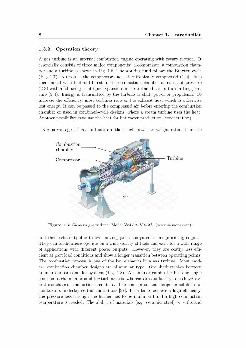
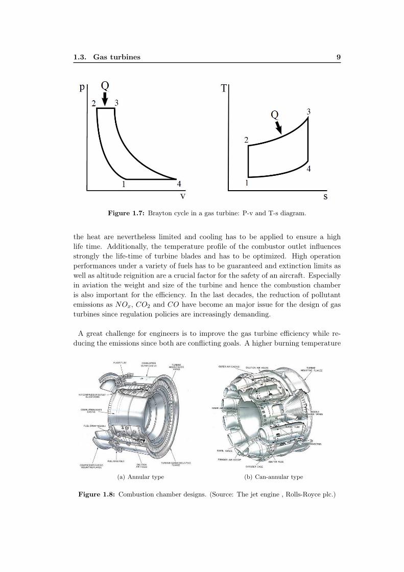
A gas turbine is an internal combustion engine operating with rotary motion. Itessentially consists of three major components: a compressor, a combustion cham-ber and a turbine as shown in Fig. 1.6. The working fluid follows the Brayton cycle(Fig. 1.7): Air passes the compressor and is isentropically compressed (1-2). It isthen mixed with fuel and burnt in the combustion chamber at constant pressure(2-3) with a following isentropic expansion in the turbine back to the starting pres-sure (3-4). Energy is transmitted by the turbine as shaft power or propulsion. Toincrease the efficiency, most turbines recover the exhaust heat which is otherwiselost energy. It can be passed to the compressed air before entering the combustionchamber or used in combined-cycle designs, where a steam turbine uses the heat.Another possibility is to use the heat for hot water production (cogeneration).
Key advantages of gas turbines are their high power to weight ratio, their size
Figure 1.6: Siemens gas turbine. Model V84.3A/V94.3A. (www.siemens.com).
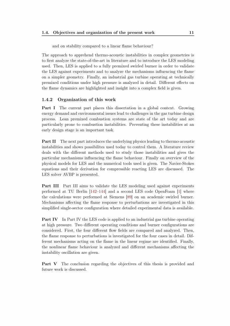
and their reliability due to less moving parts compared to reciprocating engines.They can furthermore operate on a wide variety of fuels and exist for a wide rangeof applications with different power outputs. However, they are costly, less effi-cient at part load conditions and show a longer transition between operating points.The combustion process is one of the key elements in a gas turbine. Most mod-ern combustion chamber designs are of annular type. One distinguishes betweenannular and can-annular systems (Fig. 1.8). An annular combustor has one singlecontinuous chamber around the turbine axis, whereas can-annluar systems have sev-eral can-shaped combustion chambers. The conception and design possibilities ofcombustors underlay certain limitations [97]. In order to achieve a high efficiency,the pressure loss through the burner has to be minimized and a high combustiontemperature is needed. The ability of materials (e.g. ceramic, steel) to withstand
1.3. Gas turbines 9
Figure 1.7: Brayton cycle in a gas turbine: P-v and T-s diagram.
the heat are nevertheless limited and cooling has to be applied to ensure a highlife time. Additionally, the temperature profile of the combustor outlet influencesstrongly the life-time of turbine blades and has to be optimized. High operationperformances under a variety of fuels has to be guaranteed and extinction limits aswell as altitude reignition are a crucial factor for the safety of an aircraft. Especiallyin aviation the weight and size of the turbine and hence the combustion chamberis also important for the efficiency. In the last decades, the reduction of pollutantemissions as NOx, CO2 and CO have become an major issue for the design of gasturbines since regulation policies are increasingly demanding.
A great challenge for engineers is to improve the gas turbine efficiency while re-ducing the emissions since both are conflicting goals. A higher burning temperature
(a) Annular type (b) Can-annular type
Figure 1.8: Combustion chamber designs. (Source: The jet engine , Rolls-Royce plc.)

10 Chapter 1. Introduction
increases the efficiency but leads to problems for the structure as well as to a higherformation of NOx. On the other hand NOx can be reduced by reducing the availableoxygen but this leads to an increase in carbon monoxide CO and unburnt hydrocar-bon emission due to incomplete combustion. To overcome this problem, gas turbinemanufacturers introduced the so-called lean (technically) premixed combustion sys-tems. Here, air and fuel are premixed before they enter the combustion chamberso that the air acts as a diluter in order to reduce the combustion temperatureand therefore the NOx formation. Due to a higher combustion efficiency, a reduc-tion of formed CO is also achieved. Nevertheless, these low-emission gas turbinesare known to be particularly susceptible to thermo-acoustic instabilities [97, 126],which are characterized by large pressure amplitudes and heat release oscillationsand controlled by non-linear effects [2, 3, 101]. These instabilities can lead to severeproblems like noise emission, heat flux enhancement on duct linings, global extinc-tion of the flame, structural vibrations or fatigue of burner and liner parts and eventhe failure of the turbine [174]. The prediction of this phenomenon at an earlydesign stage has become an important task, but it remains still a great challengetoday in terms of scientific modeling. This is the general framework of this PhD.
1.4 Objectives and organization of the present work
1.4.1 Objectives
The present work is placed in the framework of thermo-acoustic instabilities fo-cussing on different mechanisms affecting the stability of gas turbine chambers.Large Eddy Simulation (LES) has been widely used for the numerical simulationof turbulent flows and is recognized as a powerful tool to study thermo-acousticinstabilities [126]. Complex industrial configurations can be successfully describedby LES [136, 153] and thermo-acoustic instabilities can be captured for academicconfigurations [116, 176] and in complex industrial aeronautical combustion cham-bers [188, 189]. Nevertheless less information is available for large scale industrialgas turbines, which are typically ten times bigger than aeronautical engines andwhere the Reynolds numbers easily reach 1.000.000.
The objectives of this thesis can be summarized as follows:
• Is LES capable of handling such complex large industrial size geometries?
• Is LES modeling advanced enough to be used in industry as a design tool forgas turbine combustion chambers?
• Which mechanisms are causing thermo-acoustic instabilities? In systems withmultiple inlets for air and fuel, how can models derived for simple burners beextended?
• Thermo-acoustic instabilities are controlled by non-linear effects due to heatrelease fluctuation [2, 3, 101]. What is the effect of nonlinearity on the flame
1.4. Objectives and organization of the present work 11
and on stability compared to a linear flame behaviour?
The approach to apprehend thermo-acoustic instabilities in complex geometries isto first analyze the state-of-the-art in literature and to introduce the LES modelingused. Then, LES is applied to a fully premixed swirled burner in order to validatethe LES against experiments and to analyze the mechanisms influencing the flameon a simpler geometry. Finally, an industrial gas turbine operating at technicallypremixed conditions under high pressure is analyzed in detail. Different effects onthe flame dynamics are highlighted and insight into a complex field is given.
1.4.2 Organization of this work
Part I The current part places this dissertation in a global context. Growingenergy demand and environmental issues lead to challenges in the gas turbine designprocess. Lean premixed combustion systems are state of the art today and areparticularly prone to combustion instabilities. Preventing these instabilities at anearly design stage is an important task.
Part II The next part introduces the underlying physics leading to thermo-acousticinstabilities and shows possibilites used today to control them. A literature reviewdeals with the different methods used to study those instabilities and gives theparticular mechanisms influencing the flame behaviour. Finally on overview of thephysical models for LES and the numerical tools used is given. The Navier-Stokesequations and their derivation for compressible reacting LES are discussed. TheLES solver AVBP is presented.
Part III Part III aims to validate the LES modeling used against experimentsperformed at TU Berlin [142–144] and a second LES code OpenFoam [1] wherethe calculations were performed at Siemens [89] on an academic swirled burner.Mechanisms affecting the flame response to perturbations are investigated in thissimplified single-sector configuration where detailed experimental data is available.
Part IV In Part IV the LES code is applied to an industrial gas turbine operatingat high pressure. Two different operating conditions and burner configurations areconsidered. First, the four different flow fields are compared and analyzed. Then,the flame response to perturbations is investigated for the four cases in detail. Dif-ferent mechanisms acting on the flame in the linear regime are identified. Finally,the nonlinear flame behaviour is analyzed and different mechanisms affecting theinstability oscillation are given.
Part V The conclusion regarding the objectives of this thesis is provided andfuture work is discussed.


Part II
Theoretical background

Chapter 2
Thermo-acoustic instabilities
Contents2.1 Causes of thermo-acoustic instabilities . . . . . . . . . . . . . 16
2.2 Control of thermo-acoustic instabilities . . . . . . . . . . . . 19
2.3 Study of thermo-acoustic instabilities . . . . . . . . . . . . . 20
2.3.1 Forced response method . . . . . . . . . . . . . . . . . . . . . 20
2.3.2 Self-excitation method . . . . . . . . . . . . . . . . . . . . . . 25
2.4 CFD as a tool to study thermo-acoustic instabilities . . . . 26
The first observation of combustion oscillation dates back to 1777, when Higginsdiscovered the so-called "singing flame" [179]. In 1858 John LeConte [96] describedthe interaction between acoustics and combustion when he observed synchronousflame movement to music:
"I happened to be one of a party of eight persons assembled after tea forthe purpose of enjoying a private musical entertainment. Three instru-ments were employed in the performance of several of the grand triosof Beethoven, namely, the piano, violin and violoncello. Two ’fish-tail’gas burners projected from the brick wall near the piano. (...) Soon af-ter the music commenced, I observed that the flame of the last-mentionedburner exhibited pulsations in height which were exactly synchronous withthe audible beats. This phenomenon especially striking when the strongnotes of the violoncello came in. It was exceedingly interesting to observehow perfectly even the trills of this instrument were reflected on the sheetof flame. A deaf man might have seen the harmony."
Twenty years later in 1878, Lord Rayleigh discovered that not only the acousticshave an influence on the flame, but that a moving flame also excites acoustics [135].Since then, the field of thermo-acoustic instabilities exists, but its interest for theresearch community was limited over a long time. It only became the center ofattraction for a wider community with the development of high-intensity combus-tion systems, where suddenly unforeseen and undesired instabilities occurred. Theseinstabilities are characterized by large pressure amplitudes and heat release oscilla-tions which can lead to severe problems to the machine like noise emission, heat fluxenhancement on duct linings, global extinction of the flame, structural vibrationsor fatigue of burner and liner parts and even the failure of the turbine [174].

16 Chapter 2. Thermo-acoustic instabilities
This chapter first introduces the physical mechanisms leading to thermo-acousticinstabilities in section 2.1. Then, in section 2.2 different possibilities to controlthose instabilities are discussed. Present methods to predict thermo-acoustic in-stabilites are described (section 2.3). Finally, methods based on LES extended toinstabilities are discussed in more details (section 2.4) because they are the centerof this PhD work.
2.1 Causes of thermo-acoustic instabilities
Thermo-acoustic instabilities are the result of a resonant feedback between combus-tion, acoustic waves and flow [34] (Fig. 2.1). Gases travelling through the flame
Figure 2.1: Feedback mechanism responsible for combustion instabilities [103].
front are heated up proportionally to the heat release rate. When the heat releasefluctuates, the gases dilatation rate varies in time and the gases being heated uppush the surrounding gases outwards as they expand. This leads to an increase inlocal pressure which then propagates as acoustic waves. The flame can be comparedto an acoustic monopole [67, 170, 171] as it behaves locally as an inflating anddeflating balloon radiating sound in all directions. These pressure waves propagatethrough the domain and are reflected (dependent on the impedance) at the turbineinlet and the combustor outlet, inducing perturbations of the flow and mixture.This leads to a perturbation of heat release which basically appears in two differentways [103]:
• Variation of the flame surface area:Acoustic waves induce velocity oscillations to the flow. The accelerated anddecelerated mixture changes the flame shape accordingly, leading to variationsin the total flame surface area and hence to oscillations in the total heat release.
• Fluctuation of the heat of reaction:Acoustic waves further induce oscillations to the air and fuel inlet mass flowrates leading locally to mixture heterogeneities. These mixture variationspropagate to the flame front and influence the power released by unit of totalmass.
2.1. Causes of thermo-acoustic instabilities 17
The well-known Rayleigh criterion [113, 135] finally gives a condition for thisclosed feedback loop (Fig. 2.1) under which instabilities arise:∫
V
∫Tp′q′dV dt > 0 (2.1)
where p′ and q′ are the pressure and heat release rate fluctuations respectively, Vis the volume of the domain and T the oscillation period. The Rayleigh criterionstates that pressure and heat release oscillations must be in phase to have a growingamplitude of instability. In other words, local pressure and heat release rate mustincrease or decrease at the same time. When gases expand against a growing pressurefield, energy is transmitted to the acoustic field leading again to an increase inpressure. This happens when the phase between heat release rate and pressure isbetween −π/2 and π/2. Note that the Rayleigh criterion has to be integrated overthe domain, which means that locally pressure and heat release oscillations can bein phase, but at the same time out of phase at a different position. The exchangedenergy would thus cancel out and instabilities might be suppressed. When flamesare "compact", i.e. when the acoustic wavelength is long compared to the flamethickness this problem disappears: since pressure fluctuations are homogeneous overthe flame front, the Rayleigh criterion becomes∫
T
∫∫∫Vp′q′dV dt > 0 or
∫Tp′∫∫∫
Vq′dV dt > 0 or
∫Tp′Q′dt > 0 (2.2)
where Q′ is the total heat release in the burner. Unfortunately, we will show thatflames are not compact in the burners studied in this PhD, making their analysismore complex than suggested by Eq. 2.2.
Figure 2.2 shows the energy gain and the losses as a function of the perturba-tion in terms of the square of the acoustic velocity. The acoustic losses are assumedto be linearly increasing with the perturbation level [35] whereas the energy gainof the flame is linear for low perturbation amplitudes (region I) and saturates forlarger perturbation levels (region II). Acoustics are linear in most cases where p′/premains smaller than 1% explaining why the losses depend linearly on | u′ |2. Onthe other hand, combustion (Q′) is expected to behave nonlinearly (and this is oftenobserved [32, 123]): Q can not be negative and can not exceed values correspondingto the heat release associated to the total fuel mass introduced in the burner in oneperiod.
Figure 2.3 shows a typical time evolution of growing pressure oscillations. Whenthermo-acoustic instabilities arise, first linear oscillations appear and grow expo-nentially since the energy gain is larger than the acoustic losses. An overshootzone is often observed before the pressure amplitude reaches a plateau when thelosses balance the energy gain. This oscillation state is called "limit cycle". How-ever, instability does not necessarily occur when the Rayleigh criterion alone isfulfilled because losses also play a role [24, 113]. The boundaries of the combustion

18 Chapter 2. Thermo-acoustic instabilities
Figure 2.2: Interaction between between energy losses and gain with unsteady heat addi-tion [101].
Figure 2.3: Growth of a combustion instability to limit cycle [126].
2.2. Control of thermo-acoustic instabilities 19
chamber (e.g. walls, compressor outlet, turbine inlet) and the turbulent flow dampthe acoustic energy so that a proper instability criteria is that the Rayleigh term∫T
∫ ∫ ∫V p′q′dV dt must exceed all losses terms. Finally, even the Rayleigh term
itself has been discussed by many authors. Chu [24] or Nicoud et al. [113] investi-gated an extension to the Rayleigh criterion integrating the fluctuation of pressure,velocity and entropy. This leads to a criterion where temperature and heat release(and not pressure and heat release) must be in phase for the instability to grow.They concluded that the extended version should be used for studies on combustioninstabilities.
2.2 Control of thermo-acoustic instabilities
Thermo-acoustic instabilities should preferably be avoided at an early design stage.However, the prediction of flame-acoustic interactions is a great challenge todaybecause all mechanisms leading to an unstable behaviour of the machine are not fullyunderstood. It is therefore important, to have a posteriori methods to control andsuppress thermo-acoustic instabilities. They can be classified in two categories, bothhaving the goal to change the phase between pressure and heat release oscillations:
• Passive Control [103]:
– Operating conditions: Changes in operating conditions can have an effecton the stabilization of the flame and therefore its time response as wellas on the eigenmodes of the chamber due to a change in sound speed.
– Design changes: Acoustic eigenmodes can also be changed by modifyingthe combustion chamber geometry. Furthermore, e.g. swirler positionsor burner outlets have an impact on the time response.
– Acoustic dampers [126]: Resonators can be used to damp eigenfrequen-cies. Nevertheless, frequencies encountered in most gas turbines are lowand dampers with large volumes are needed. Since space is generallylimited, the installation of these dampers is difficult in practice.
• Active Control [103, 107]:Active control techniques monitor the combustion system in order to detectthe characteristics of the instabilities in terms of frequency and amplitude.The phase difference between acoustics and heat release can now be adjustedby attenuating e.g. the fuel mass rate. Thermo-acoustic instabilities are finallysuppressed by a closed feedback loop. These systems need to be redundantsince its failure risks an instability to grow and the machine to fail.
Despite multiple academic proofs of the efficiency of active control methods [9, 11,92], active control has been used only a few times in real gas turbines [160]. The mainreason for this is that the certification and the cost of these methods remain difficult

20 Chapter 2. Thermo-acoustic instabilities
issues and that they do not control all unstable modes. Using passive methods, whichmeans building systems which are naturally stable is the preferred path today forindustry. This can be achieved only when mechanisms are understood: this explainswhy prediction methods must be developed first.
2.3 Study of thermo-acoustic instabilities
Preventing thermo-acoustic instabilities is an important task and their predictionat an early design stage remains a challenge, since their underlying mechanismsare not fully understood yet. Generally, two methods exist to study instabilities incombustors [126](Fig. 2.4):
• Forced response:The feedback loop leading to thermo-acoustic instability is removed and theflame is excited in a forced controlled mode to measure its response. Thermo-acoustic instability models give then information about stability and limitcycle oscillation amplitudes.
• Self-excited modes:The feedback loop is closed and the flow resonates on its own. The configura-tion is dominated by its own instability mode.
Figure 2.4: Forced (left) and self-excited (right) strategies to study thermo-acoustic in-stabilities [126].
2.3.1 Forced response method
In the forced response method a perturbation is introduced to the flame and itsresponse is analyzed. To do so, a common approach for acoustically compact flamescan be found in the literature which was first introduced by Crocco [29, 30]. In thisapproach, the Flame Transfer Function (FTF) is the key parameter and is definedas the ratio of the relative heat release fluctuation (q/q) to the relative inlet velocityperturbation (u/u) issued by the acoustic field. In the frequency domain it writes
F (ω) =q/q
u/u. (2.3)
with ω being the angular frequency. The FTF is generally expressed in terms of gainn = |F (ω)| and time delay τ = Arg(F (ω)/(2πf)). The shape of the FTF depends

2.3. Study of thermo-acoustic instabilities 21
on the flame shape [79] as well as on the operating conditions [85]. Flame TransferFunctions have been extensively studied in laminar and turbulent flames where onlythe axial velocity perturbation is at play. Investigations of laminar conical flamesperformed by Durox et al. [38] and Karimi et al. [76], inverted conical by Duroxet al. [38] and multi-slit conical flames studied by Kornilov et al. [85] revealed thatthe FTF gain shows a low pass filter behaviour. Schuller et al. [150] observed fromlaminar flames and Armittage et al. [2] from turbulent V-flames an overshoot in gainand associated this to vortex roll-up at the flame base. In all cases, the gain is unityin the limit of zero frequency as derived by Polifke and Lawn [127] from the globalconservation laws. The phase of the FTF evolves in these cases in an almost linearway with the frequency, indicating that the axial velocity perturbations propagateconvectively from the burner outlet to the flame. Concerning different operatingconditions, Kornilov et al. [85] showed that with increasing inlet velocity the gaindecreases at higher frequency and that phase saturation occurs at higher frequency.Kim et al. [79] and Palies et al. [116] used the Strouhal number as dimensionlessparameter instead of the frequency.
Industrial configurations use swirlers in order to create a vortex breakdown [106]which stabilizes the flame. The gain of swirled flames plotted versus frequencyusually shows a second peak. Straub and Richards [173] first noticed a strong im-pact of the swirler position on the combustion oscillations. Hirsch et al. [59] henceinvestigated the effect of swirler designs and found that an additional time lag isresponsible for changes in the FTF. Komarek et al. [84] investigated the influenceof several swirler positions on the FTF and concluded that disturbances propagateat a convective and an acoustic speed downstream the swirler position. Finally,Palies et al. [117, 119] have shown that the acoustic perturbations reaching theswirler generate transverse velocity fluctuations which are convected by the flow.As a results, swirl number perturbations occur and effect the flame angle. Whenboth components are in phase, the swirl number perturbations are small and theflame angle is less affected leading to an overshoot in gain since axial and azimuthalcomponent are acting simultaneously on the flame. Vice versa, high swirl fluctu-ations occur when both components are out of phase leading to a low flame response.
The academic configurations mentioned above run under perfectly premixed con-ditions: fuel and air are mixed far upstream of the combustion chamber. However,industrial combustion systems operate for security reasons under technically pre-mixed conditions meaning that fuel and air are mixed just prior to combustion.Thus, in technically premixed configurations another mechanisms, the perturbationof mixture, occurs and changes the shape of the FTF gain [104]. Schuermans etal. [148] compared the measured transfer matrix of a turbulent flame for a techni-cally premixed and a fully premixed system and found the maximal amplitude toincrease for the technically premixed case where equivalence ratio perturbations arepresent. Kim et al. [82] also found a phase difference between equivalence ratio andvelocity at the combustor inlet. Following Kim et al. [82] this has an impact on the
22 Chapter 2. Thermo-acoustic instabilities
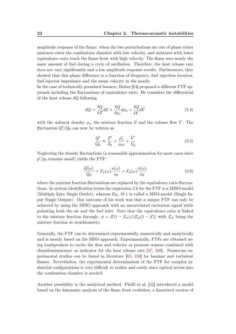
amplitude response of the flame: when the two perturbations are out of phase richermixtures enter the combustion chamber with low velocity, and mixtures with lowerequivalence ratio reach the flame front with high velocity. The flame sees nearly thesame amount of fuel during a cycle of oscillation. Therefore, the heat release ratedoes not vary significantly and a low amplitude response results. Furthermore, theyshowed that this phase difference is a function of frequency, fuel injection location,fuel injector impedance and the mean velocity in the nozzle.In the case of technically premixed burners, Huber [64] proposed a different FTF ap-proach including the fluctuations of equivalence ratio. He considers the differentialof the heat release dQ following
dQ =δQ
δZdZ +
δQ
δρudρu +
δQ
δVdV (2.4)
with the unburnt density ρu, the mixture fraction Z and the volume flow V . Thefluctuation Q′/Q0 can now be written as
Q′
Q0≈ Z ′
Z0+
ρ′uρu0
+V ′
V0
(2.5)
Neglecting the density fluctuations (a reasonable approximation for most cases sincep′/p0 remains small) yields the FTF:
Q(ω)
Q0= Fu(ω)
u(ω)
u0+ Fφ(ω)
φ(ω)
φ0(2.6)
where the mixture fraction fluctuations are replaced by the equivalence ratio fluctua-tions. In system identification terms the expression 2.6 for the FTF is a MISO-model(Multiple Inlet Single Outlet), whereas Eq. 10.1 is called a SISO-model (Single In-put Single Output). One outcome of his work was that a unique FTF can only beachieved by using the MISO approach with an uncorrelated excitation signal whilepulsating both the air and the fuel inlet. Note that the equivalence ratio is linkedto the mixture fraction through: φ = Z(1 − Zst)/(Zst(1 − Z)) with Zst being themixture fraction at stoichiometry.
Generally, the FTF can be determined experimentally, numerically and analyticallyand is mostly based on the SISO approach. Experimentally, FTFs are obtained us-ing loudspeakers to excite the flow and velocity or pressure sensors combined withchemiluminescence as indicator for the heat release rate [37, 168]. Numerous ex-perimental studies can be found in literature [63, 103] for laminar and turbulentflames. Nevertheless, the experimental determination of the FTF for complex in-dustrial configurations is very difficult to realize and costly since optical access intothe combustion chamber is needed.
Another possibility is the analytical method. Fleifil et al. [42] introduced a modelbased on the kinematic analysis of the flame front evolution, a linearized version of
2.3. Study of thermo-acoustic instabilities 23
the G-equation, for conical flames at small perturbation amplitude. It was extendedby Ducruix et al. [37] to any flame tip angle and Schuller et al [150] further developedthis approach for high frequencies and applied it to a conical and a V-flame. Goodagreement with experiments was found and the FTF could finally be determined bythe use of reduced frequency depending on the flametube radius, the flame speedand the flame angle. This modeling has been extended to the nonlinear responseof premixed flames by Lieuwen [100]. For more complex flames, Palies et al. [119]recently extended this approach to premixed swirled flames. Two additional param-eters are introduced in his model accounting for swirl number fluctuations which cannot be determined analytically: they need experiments or an adjustment process.
Another theoretical model is based on the analysis of the unit impulse responseof the flame and has been formulated by Komarek and Polifke [84] for a premixedswirled flame. The response of the flame to an axial perturbation is modeled asa Gaussian time lag distribution F (ω)axial = e−iωτ1−1/2ωσ2
1 and the response to afluctuation of swirl with F (ω)swirl = e−iωτ2−1/2ωσ2
2 − e−iωτ3−1/2ωσ23 . The FTF is
finally F (ω) = F (ω)axial + F (ω)swirl. The values for ni, τi and σi were determinedvia fitting to experimental data. Schuermanns et al. [148] used the same approachto account for mixture fluctuations in a non-swirled configuration and introducedone additional Gaussian time lag. Although good agreement is found for the fittedFTF with experiments, an a priori determination of the FTF is not possible.
Alternatively, the FTF can be determined from a computational fluid dynamics(CFD) simulation [51, 85, 175]. In this approach an unsteady CFD calculation isperformed and controlled excitations are imposed in order to generate time seriesof velocity and heat release rate oscillation. Then, the data is post-processed usingsystem identification techniques to obtain the FTF [64, 74, 105].
Once the FTF is determined, it serves as input to linear thermo-acoustic insta-bility models in order to determine the stability of the system. One approach isto model the relevant configuration as a 1D network of acoustic elements and todetermine the acoustic pressure and velocity through each element via a transfermatrix [50, 80, 129, 149]. The linearized conservation equations are solved in thefrequency domain and the complex eigenfrequencies give finally the growth rates,hence information on the stability, of the different modes. A second 1D possibil-ity is to solve the thermo-acoustic problem in the time domain with the modifiedGalerkin approach [31, 33, 36, 88, 190] which is essentially based on the use ofGreen’s functions. The acoustic mode shapes are determined from a homogeneousHelmholtz equation and they are then perturbed in the time domain. This leadsfinally to a temporal solution with growing or decaying oscillations. Eigenmodeshapes and growth rates can also be determined in 3D while solving the inhomo-geneous Helmholtz equation on 3D meshes [112, 152, 164]. In this method, a localFTF is used as input and is linked to the global FTF with amplitude n and time
24 Chapter 2. Thermo-acoustic instabilities
delay τ through:
ne−iωτ =
∫∫∫V
nl(~x)e−iωτl(~x) (2.7)
with the local amplitude nl(~x) and the local time delay τl(~x). The local FTF fieldallows as well to obtain further insight into the flame dynamics as it illustrates howthe flame reacts in different regions. The inhomogeneous Helmholtz equation canalso be solved in 3D directly in the time domain [120]. Similar to the approach inthe frequency domain, the mode shapes are finally determined.
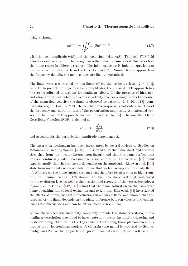
The limit cycle is controlled by non-linear effects due to heat release [2, 3, 101].In order to predict limit cycle pressure amplitudes, the classical FTF approach hasfirst to be adjusted to account for nonlinear effects. In the presence of high per-turbation amplitudes, when the acoustic velocity reaches a magnitude of the orderof the mean flow velocity, the flame is observed to saturate [2, 3, 101, 118] (com-pare also region II in Fig. 2.2). Hence, the flame response is not only a function ofthe frequency any more but also of the perturbation amplitude. An extended ver-sion of the linear FTF approach has been introduced by [35]: The so-called FlameDescribing Function (FDF) is defined as
F (ω, u) =q′/q
u′/u. (2.8)
and accounts for the perturbation amplitude dependence u.
The saturation mechanism has been investigated by several reviewers. Studies onV-flames and swirling flames [3, 40, 118] showed that the flame sheet and the vor-tices shed from the injector interact non-linearly and that the flame surface areaevolves non-linearly with increasing excitation amplitude. Durox et al. [40] foundexperimentally that the response is dependent on the amplitude. Lieuwen et al. [101]state from investigations on a swirled flame that vortex roll-up and unsteady flamelift-off decrease the flame surface area and lead therefore to saturation at higher am-plitudes. Thumuluru et al. [178] showed that the flame shape is strongly influencedby the excitation level as well as the position and strength of the vortex breakdownregion. Schimek et al. [142, 143] found that the flame saturation mechanisms wereflame quenching due to local extinction and re-ignition. Kim et al. [81] investigatedthe effects of equivalence ratio fluctuations in a swirled flame and showed that theresponse of the flame depends on the phase difference between velocity and equiva-lence ratio fluctuations and can be either linear or non-linear.
Linear thermo-acoustic instability tools only provide the stability criteria, but anonlinear description is required to investigate limit cycles, instability triggering andmode switching. The FDF is the key element determining those phenomena and isused as input for nonlinear models. A Galerkin type model is proposed by Selime-fendigil and Polifke [151] to predict the pressure oscillation amplitude in a Rijke tube.
2.3. Study of thermo-acoustic instabilities 25
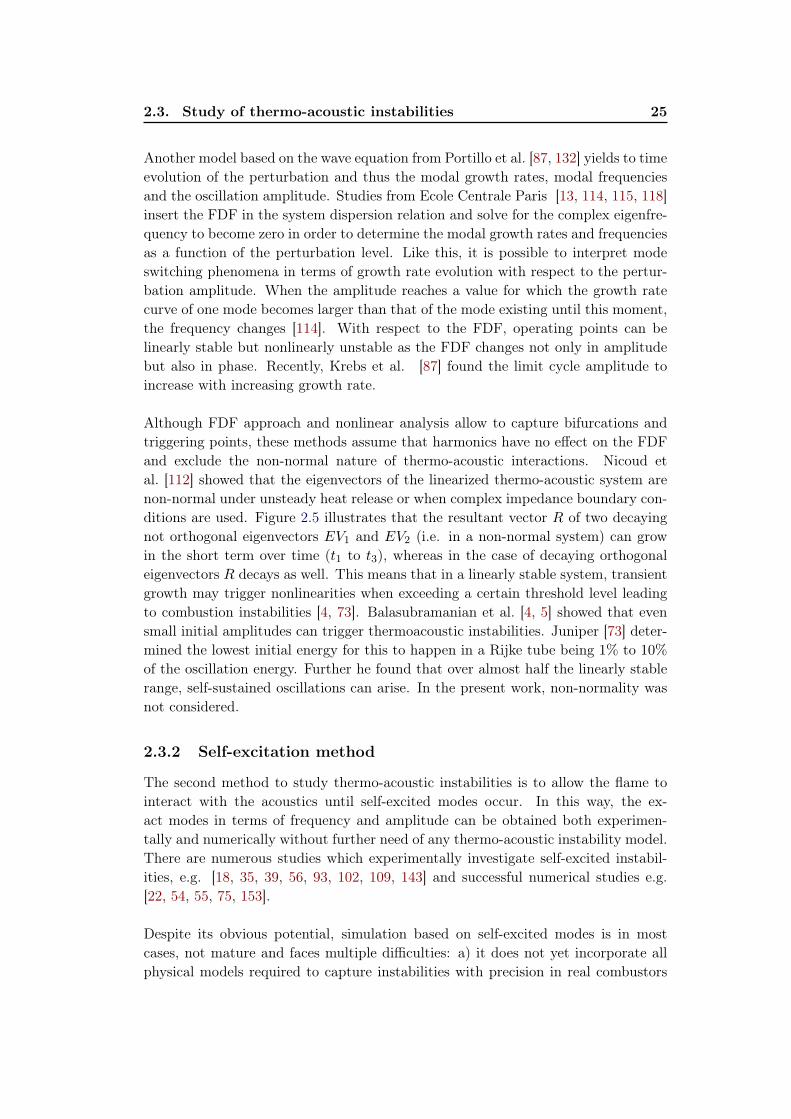
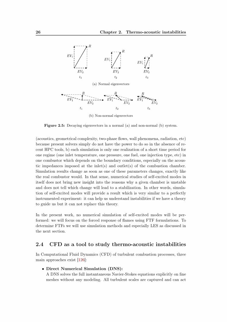
Another model based on the wave equation from Portillo et al. [87, 132] yields to timeevolution of the perturbation and thus the modal growth rates, modal frequenciesand the oscillation amplitude. Studies from Ecole Centrale Paris [13, 114, 115, 118]insert the FDF in the system dispersion relation and solve for the complex eigenfre-quency to become zero in order to determine the modal growth rates and frequenciesas a function of the perturbation level. Like this, it is possible to interpret modeswitching phenomena in terms of growth rate evolution with respect to the pertur-bation amplitude. When the amplitude reaches a value for which the growth ratecurve of one mode becomes larger than that of the mode existing until this moment,the frequency changes [114]. With respect to the FDF, operating points can belinearly stable but nonlinearly unstable as the FDF changes not only in amplitudebut also in phase. Recently, Krebs et al. [87] found the limit cycle amplitude toincrease with increasing growth rate.
Although FDF approach and nonlinear analysis allow to capture bifurcations andtriggering points, these methods assume that harmonics have no effect on the FDFand exclude the non-normal nature of thermo-acoustic interactions. Nicoud etal. [112] showed that the eigenvectors of the linearized thermo-acoustic system arenon-normal under unsteady heat release or when complex impedance boundary con-ditions are used. Figure 2.5 illustrates that the resultant vector R of two decayingnot orthogonal eigenvectors EV1 and EV2 (i.e. in a non-normal system) can growin the short term over time (t1 to t3), whereas in the case of decaying orthogonaleigenvectors R decays as well. This means that in a linearly stable system, transientgrowth may trigger nonlinearities when exceeding a certain threshold level leadingto combustion instabilities [4, 73]. Balasubramanian et al. [4, 5] showed that evensmall initial amplitudes can trigger thermoacoustic instabilities. Juniper [73] deter-mined the lowest initial energy for this to happen in a Rijke tube being 1% to 10%
of the oscillation energy. Further he found that over almost half the linearly stablerange, self-sustained oscillations can arise. In the present work, non-normality wasnot considered.
2.3.2 Self-excitation method
The second method to study thermo-acoustic instabilities is to allow the flame tointeract with the acoustics until self-excited modes occur. In this way, the ex-act modes in terms of frequency and amplitude can be obtained both experimen-tally and numerically without further need of any thermo-acoustic instability model.There are numerous studies which experimentally investigate self-excited instabil-ities, e.g. [18, 35, 39, 56, 93, 102, 109, 143] and successful numerical studies e.g.[22, 54, 55, 75, 153].
Despite its obvious potential, simulation based on self-excited modes is in mostcases, not mature and faces multiple difficulties: a) it does not yet incorporate allphysical models required to capture instabilities with precision in real combustors
26 Chapter 2. Thermo-acoustic instabilities
(a) Normal eigenvectors
(b) Non-normal eigenvectors
Figure 2.5: Decaying eigenvectors in a normal (a) and non-normal (b) system.
(acoustics, geometrical complexity, two-phase flows, wall phenomena, radiation, etc)because present solvers simply do not have the power to do so in the absence of re-cent HPC tools, b) each simulation is only one realization of a short time period forone regime (one inlet temperature, one pressure, one fuel, one injection type, etc) inone combustor which depends on the boundary conditions, especially on the acous-tic impedances imposed at the inlet(s) and outlet(s) of the combustion chamber.Simulation results change as soon as one of these parameters changes, exactly likethe real combustor would. In that sense, numerical studies of self-excited modes initself does not bring new insight into the reasons why a given chamber is unstableand does not tell which change will lead to a stabilization. In other words, simula-tion of self-excited modes will provide a result which is very similar to a perfectlyinstrumented experiment: it can help us understand instabilities if we have a theoryto guide us but it can not replace this theory.
In the present work, no numerical simulation of self-excited modes will be per-formed: we will focus on the forced response of flames using FTF formulations. Todetermine FTFs we will use simulation methods and especially LES as discussed inthe next section.
2.4 CFD as a tool to study thermo-acoustic instabilities
In Computational Fluid Dynamics (CFD) of turbulent combustion processes, threemain approaches exist [126]:
• Direct Numerical Simulation (DNS):A DNS solves the full instantaneous Navier-Stokes equations explicitly on finemeshes without any modeling. All turbulent scales are captured and can act

2.4. CFD as a tool to study thermo-acoustic instabilities 27
on the combustion process leading to high numerical costs.
• Large Eddy Simulation (LES):A LES resolves the turbulent large scale structures and models the small scaleones by applying a filter. Unsteady features are represented and the modelingimpact is reduced. Lower numerical costs than DNS.
• Reynolds-Averaged-Navies-Stokes (RANS):RANS simulations compute only averaged values without solving turbulentquantities. Coarse grids can be used and the numerical costs are reducedcompared to LES.
LES is an intermediate approach which includes unsteady features with a reducedimpact of the required modeling and acceptable computational costs. NumerousLES have been performed for laboratory and industry-scale configurations and haveproved the capability of this approach [74, 153, 166, 176, 189]. Another advantage ofLES is that it is well suited to unsteady phenomena such as forced flames requiredfor FTFs. Therefore, the LES approach is used throughout this thesis.
Thermo-acoustic instabilities can be studied with the forced response method oras self-excited modes. For both approaches, the LES needs to meet special require-ments. In the forced response method, first a stable regime has to be attained beforea controlled excitation signal is introduced. The size of the forced domain needs tobe reduced in order to exclude any possible resonant frequencies arising from thegeometry. Specific boundary conditions are also needed to avoid unnatural resonantmodes [78, 154]. One drawback is that transverse acoustic modes can not be pre-dicted as they are created inside the chamber itself. For the self-excitation methodthe whole combustor geometry has to be taken into account. In order to generateresonance, the acoustic boundary conditions at the in- and outlet need to be welldefined, something which is difficult in a real turbine. With this method, the limitcycles (modal frequency and amplitude) are determined from the LES exactly asthey appear in experiments and all modes are captured. Nevertheless, if only oneboundary condition is not accurately set, no limit cycle or a different one could bepredicted.
In terms of computational costs the forced response method is the better choice.Self-excited oscillations may require a long computing time, first because the simu-lation domain has to describe the entire combustor and second because limit cyclesneed to be simulated over several periods to reach convergence. Furthermore, hys-teresis and transition from stable to unstable operation condition can take a longphysical time which is out of reach of present CPU power. Moreover, some com-bustors are linearly stable but non-linearly unstable meaning that a perturbationhas to be added in order to start a growing oscillation. The choice of the initialcondition for such LES is difficult and CPU intense as many tests are required. Theforced response method is much faster to compute since the computational domain

28 Chapter 2. Thermo-acoustic instabilities
(a) Self-excitation method
(b) Forced response method
Figure 2.6: Schematic drawing of self-excited and forced response method.
is smaller and less oscillation periods need to be calculated. The CPU time for asubsequent analysis with any thermo-acoustic instability code is negligible comparedto the LES computations. Figure 2.6 summarized both methods.
During this dissertation, the flame transfer function and the mechanisms at playleading to stable or unstable combustor behaviour are determined with the forcedresponse method. The LES code AVBP [110, 145, 157]1 is used and is described inthe next chapter.
1http://www.cerfacs.fr/
Chapter 3
Numerical method
Contents3.1 Governing equations . . . . . . . . . . . . . . . . . . . . . . . . 30
3.1.1 Equation of state . . . . . . . . . . . . . . . . . . . . . . . . . 30
3.1.2 Species transport . . . . . . . . . . . . . . . . . . . . . . . . . 31
3.1.3 Chemistry modeling . . . . . . . . . . . . . . . . . . . . . . . 31
3.2 Large-Eddy Simulation . . . . . . . . . . . . . . . . . . . . . . 32
3.2.1 Filtered Navier-Stokes equations . . . . . . . . . . . . . . . . 32
3.2.2 Sub-grid scale modeling . . . . . . . . . . . . . . . . . . . . . 34
3.2.3 Combustion modeling . . . . . . . . . . . . . . . . . . . . . . 35
3.3 Discretization . . . . . . . . . . . . . . . . . . . . . . . . . . . . 36
3.3.1 Cell-vertex method . . . . . . . . . . . . . . . . . . . . . . . . 36
3.3.2 Time advancement . . . . . . . . . . . . . . . . . . . . . . . . 36
3.3.3 Convection scheme . . . . . . . . . . . . . . . . . . . . . . . . 36
3.4 Boundary conditions . . . . . . . . . . . . . . . . . . . . . . . 37
3.4.1 Inlet and outlet boundary conditions . . . . . . . . . . . . . . 37
3.4.2 Wall treatment . . . . . . . . . . . . . . . . . . . . . . . . . . 38
3.5 LES and System identification . . . . . . . . . . . . . . . . . . 39
3.5.1 Excitation signal . . . . . . . . . . . . . . . . . . . . . . . . . 39
3.5.2 System identification . . . . . . . . . . . . . . . . . . . . . . . 40
The present part is organized as follows: This chapter describes the governingequations solved by the LES code AVBP used throughout this thesis. AVBP isa massively parallel LES code solving the filtered, compressible, reacting Navier-Stokes equations on three-dimensional unstructured grids [26, 139, 146]. The codeis only shortly described here, since no specific developments have been made duringthis work. The interested reader is referred to [110, 145, 157].The next chapter deals with specific details of the analysis of thermo-acoustic in-stabilities. In particular, the excitation signals used for flame identification (FTFs)are discussed and the system identification process is described.

30 Chapter 3. Numerical method
3.1 Governing equations
The evolution of a compressible and reacting flow is defined by the momentum,energy and species balance equations and can be written as:
∂ρui∂t
+∂ρuiuj∂xj
= − ∂
∂xj[pδij − τij ] (3.1)
∂ρE
∂t+∂ρEuj∂xj
= − ∂
∂xj[ui (pδij − τij) + qi] + ωT (3.2)
∂ρYk∂t
+∂ρujYk∂xj
= − ∂
∂xj[Jj,k] + ωk (3.3)
where ρ, ui, p and E are respectively the mass density, the i-th component of thevelocity vector, the thermodynamic pressure and the energy per mass unit (specificinternal and kinetic energy). The index notation is adopted (Einstein summationconvention) for almost all the variables and equations. The exception concerns theindex k that is related to species and traditional summation symbol is used in thiscase, and N is the related number of species. Yk is the mass-fraction of speciesk. The Kronecker’s delta is δij . Assuming the fluid to be Newtonian (viscousstress tensor is linearly dependent of the strain rate tensor) and neglecting the bulkviscosity, the viscous stress tensor τij results:
τij = 2µ
(Sij −
1
3Sll
)(3.4)
with µ the shear dynamic viscosity and Sij the strain rate tensor defined as:
Sij =1
2
(∂ui∂xj
+∂uj∂xi
)(3.5)
The heat and molecular diffusion fluxes are qj and Jj,k respectively. The source termωT is related to the heat release rate and ωk to the production rate of the species k.
E is the total (non-chemical) energy per unit mass calculated as E = H − P/ρ.H represents the total enthalpy calculated as H = hs + 1
2uiui, where12uiui is the
kinetic energy of the gases and hs =∫ TT0CpdT is the sensible enthalpy, Cp and T
being the heat capacity and temperature of the mixture respectively.
3.1.1 Equation of state
The equation of state follows the ideal gas law:
P = ρTR0
W(3.6)
where R0 is the universal gas constant and W is the mean molecular weight of thegas mixture.

3.1. Governing equations 31
3.1.2 Species transport
The conservation of mass has to be satisfied and follows:
N∑k=1
YkVki = 0 (3.7)
where V ki is the diffusion velocity of species k in directions i = 1, 2, 3 for the number
of N species. The determination of diffusion velocities for all species requires acomplex non-linear system of equations [10, 41, 126, 185] and the solution is timeconsuming. Therefore a simplified approach is used in AVBP to solve the chemicalspecies transport following the Hirschfelder and Curtiss approximation [60]:
YkVki = −Dk
Wk
W
∂Xk
∂xi(3.8)
with Dk, Wk and Xk being the averaged diffusion coefficient into the mixture, themolar weight and the molar fraction of species k respectively. Since this approxima-tion is not mass conservative, a correction velocity V c
i is added in the conservationequation for each species (Eq. 3.7) resulting in the species diffusion flux for speciesk:
Ji,k = −ρ(Dk
Wk
W
∂Xk
∂xi− YkV c
i
)(3.9)
where the diffusivity Dk = Dth/Lek, with Dth being the thermal diffusivity of themixture. Lek is the Lewis number of species k and is assumed to be constant [126].
3.1.3 Chemistry modeling
The chemistry is determined for M reactions and N reactantsMk:
N∑k=1
ν ′kjMk N∑k=1
ν ′′kjMk, j = 1,M (3.10)
where ν ′kj and ν′′kj are the stoichiometric coefficients. The reaction rate progress Qj
of reaction j is
Qj = Kf,j
N∏k=1
(ρYkWk
)ν′kj−Kr,j
N∏k=1
(ρYkWk
)ν′′kj(3.11)
with the forward and reverse rate Kf,j and Kr,j of reaction j respectively.
The reaction rates follow the Arrhenius law
Kf,j = Af,jexp
(−Ea,jR0T
)(3.12)
32 Chapter 3. Numerical method
with Af,j and Ea,j denoting the pre-exponential constant and the activation energyof reaction j. The reverse reaction rate writes
Kr,j = Kr,j/Keq (3.13)
using the equilibrium constant Keq [90]. The reaction rate of species k finally follows
ωk = Wk
M∑j=1
(ν ′kj − ν ′′kj
)Qj (3.14)
and the formation enthalpy of species k, ∆h0f,k can be written as:
ωT = −N∑k=1
ωk∆h0f,k (3.15)
3.2 Large-Eddy Simulation
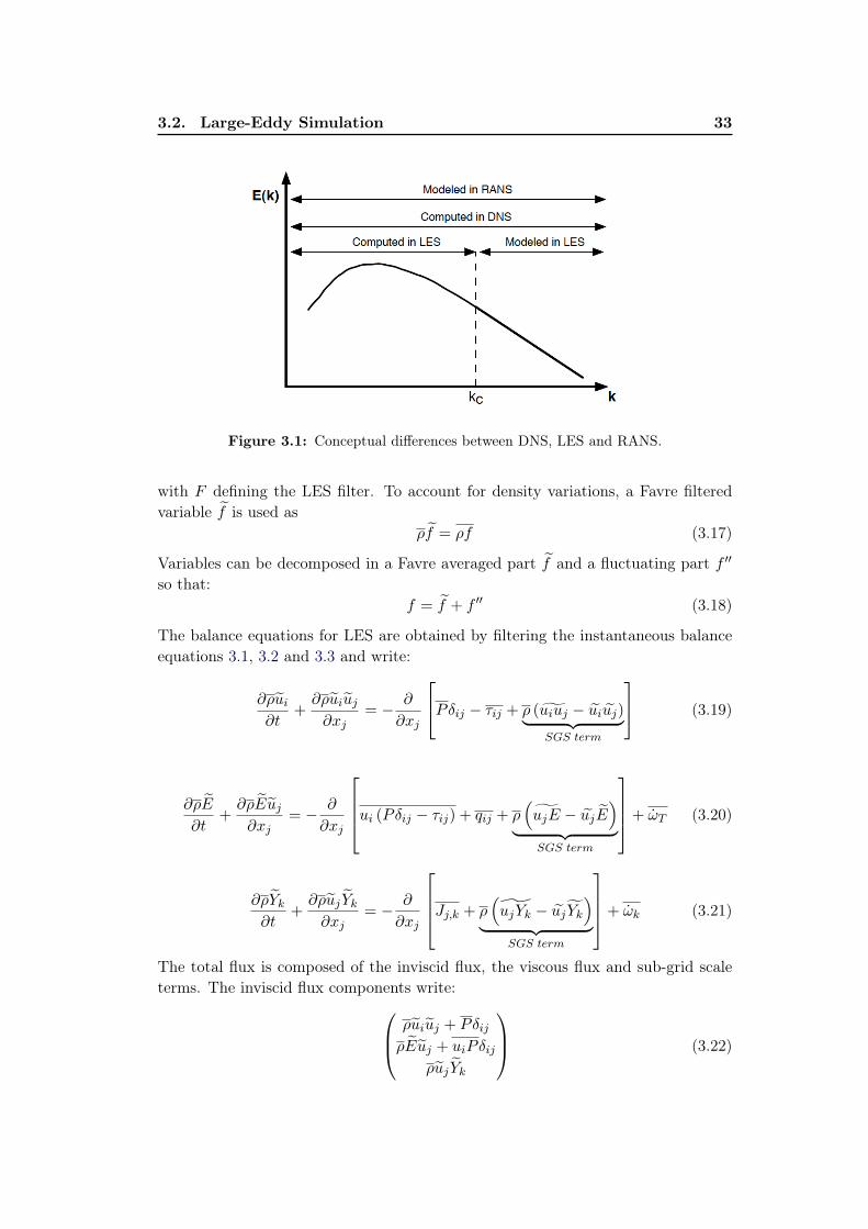
Large Eddy Simulation (LES) [130] is a widely recognized approach to compute thecharacteristics of turbulent flows. It is compared to the Direct Numerical Simulation(DNS) and the classical Reynolds Averaged Navier-Stokes (RANS) and intermediateapproach. Figure 3.1 illustrates the different concepts of DNS, LES and RANSshowing the spectral density of the turbulent kinetic energy E(K) over the turbulentwave number k. DNS resolves the entire range of turbulent length scales and doesnot need any models but is expensive in terms of CPU cost. For RANS and LES newgoverning equations are derived by introducing operators to the set of compressibleNavier-Stokes equations whereby unclosed terms arise. Hence, models are needed inorder to solve the equations. The major differences between RANS and LES resultfrom the operator used for the derivation. The RANS approach uses a temporal orensemble average over the studied flow [21, 130] and the unclosed terms representthe physics taking place over the entire range of frequencies. In other words, theentire range of turbulent length scales is modeled. The operator in LES is a spatiallylocalized time independent filter of given size ∆. This "spatial average" separatesthe large scales (greater than the filter size) from the small scales (smaller thanthe filter size) so that the unclosed terms represent the physics associated withthe small structures at high frequencies. LES represents the dynamic large scalemotions which are critical in complex gas turbine engines [126]. It is therefore thebest approach considering CPU cost and accuracy for combustion instabilities.
3.2.1 Filtered Navier-Stokes equations
To obtain the new set of equations a spatial filtering operator is introduced [126]
f(x) =
∫f(x′)F (x− x′)dx′ (3.16)
3.2. Large-Eddy Simulation 33
Figure 3.1: Conceptual differences between DNS, LES and RANS.
with F defining the LES filter. To account for density variations, a Favre filteredvariable f is used as
ρf = ρf (3.17)
Variables can be decomposed in a Favre averaged part f and a fluctuating part f ′′
so that:f = f + f ′′ (3.18)
The balance equations for LES are obtained by filtering the instantaneous balanceequations 3.1, 3.2 and 3.3 and write:
∂ρui∂t
+∂ρuiuj∂xj
= − ∂
∂xj
Pδij − τij + ρ (uiuj − uiuj)︸ ︷︷ ︸SGS term
(3.19)
∂ρE
∂t+∂ρEuj∂xj
= − ∂
∂xj
ui (Pδij − τij) + qij + ρ(ujE − ujE
)︸ ︷︷ ︸
SGS term
+ ωT (3.20)
∂ρYk∂t
+∂ρuj Yk∂xj
= − ∂
∂xj
Jj,k + ρ(ujYk − uj Yk
)︸ ︷︷ ︸
SGS term
+ ωk (3.21)
The total flux is composed of the inviscid flux, the viscous flux and sub-grid scaleterms. The inviscid flux components write: ρuiuj + Pδij
ρEuj + uiPδijρuj Yk
(3.22)

34 Chapter 3. Numerical method
and the viscous flux is −τij− (uiτij) + qij
Jj,k
(3.23)
The convective terms introduce additional terms in the conservation equations dur-ing filtering due to their non-linear character.−τij tqij
t
Jj,kt
=
ρ (uiuj − uiuj)ρ(ujE − ujE
)ρ(ujYk − uj Yk
) (3.24)
Those terms represent the contribution of the non-resolved turbulent scales whichhave to be modeled.
3.2.2 Sub-grid scale modeling
Filtering the transport equations yields a closure problem for the sub-grid scale(SGS) turbulent fluxes. The influence of the SGS on the resolved motion is taken intoaccount by a model based on the introduction of a turbulent viscosity νt followingthe Boussinesq hypothesis [14] assuming the SGS terms to behave as their laminarcounterparts, except with the use of a turbulent viscosity νt instead of the gasviscosity. The Reynolds tensor writes:
τ tij = 2ρνtSij −1
3δijτ
tll (3.25)
Note that this approach assumes that the SGS field has a purely dissipative effect.The heat and species turbulent flux terms, the turbulent thermal and species diffu-sivities are computed using constant turbulent Prandtl and Schmidt numbers.
The eddy viscosity is calculated using the Smagorinsky [161] turbulence modelwhere νt is proportional to the resolved filtered strain tensor Sij and the meshsize ∆ = V
1/3cell . It is given through
νt = (CS∆)2√
2SijSij (3.26)
CS is the model constant and takes typically values between 0.1 and 0.18 and is fixedduring this work to 0.18. The Smagorinsky model was developed in the 1960’s [161]and is extensively tested over a wide range of flow configurations. It is easy toimplement and performs sufficiently well for flows away from solid walls at lowcomputational cost. Furthermore, it supplies the right amount of kinetic energydissipation in homogeneous isotropic turbulent flows. However, locality is lost andonly global quantities are maintained. and it is known as being too dissipative.Particularly, the simulation of wall-bounded flows combined with no-slip boundaryconditions leads to an over prediction of the fluid friction on walls. The reason isthat νt is proportional to the velocity gradients and is over predicted. The use of

3.2. Large-Eddy Simulation 35
slip-wall-law boundary conditions avoids this problem and justifies the use of theSmagorinsky model.
3.2.3 Combustion modeling
One problem occurring in LES is that the flame thickness is generally smaller thanthe mesh size and cannot be resolved. For this reason, the Dynamic ThickenedFlame Model (DTFM) introduced by Légier [98, 145, 156] is used to model turbulentcombustion. It is based on a classical dimensional analysis of premixed flames [185]showing the dependence of the flame front thickness δ
δ ∝√D
A(3.27)
and the laminar flame speed SL
SL ∝ D ·A (3.28)
on the reaction rate pre-exponential constant A and the diffusion coefficient D. Thismodel is developed in order to resolve the flame front smaller than the mesh size bymultiplying it with a thickening factor F while preserving the flame speed SL. Theconstant A is therefore divided and D multiplied by F . The thickening reduces theability of the vortices to wrinkle the flame front. This results in a reduced reactionrate since the flame surface is decreased which is shown in Fig. 3.2. The efficiency
(a) Non-thickened flame (b) Thickened flame
Figure 3.2: Direct Numerical Simulation of flame/turbulence interaction [126].
function E by Charlette et al. [20] is used to account for these effects and multipliesthe diffusion and reaction terms by the factor E:
E =
(1 +min
[∆
δ0l
,Γ
(∆
δ0l
,u′∆s0l
, Re∆
)])β(3.29)
36 Chapter 3. Numerical method
Here, ∆ defines the implicit filter size of the LES, u′∆ the SGS root-mean-squarevelocity. The propagation velocity and the thickness of the corresponding laminarflame are s0
l and δ0l . The Reynolds number follows Re∆ = s0
l δ0l ν, with ν being the
viscosity of the fresh gases and the model parameter is β.
3.3 Discretization
The LES code AVBP is used for simulations performed during this work. It is ahighly massively parallel code which solves compressible Navier-Stokes equations ona unstructured grids [147, 165]. This section presents shortly the cell-vertex methodand the numerical schemes used in this thesis. Details about the numerics can befound in [91].
3.3.1 Cell-vertex method
AVBP is based on the "finite volume" (FV) method wich can be implemented inthree different ways: cell-centered, vertex-centered and the cell-vertex method. Onlythe latter is discussed here, since it is used in AVBP. In the cell-vertex technique thediscrete values of the conserved variables are stored at the cell vertices and the meanvalues of the fluxes are obtained by averaging over the cell edges. The first step ofthe cell-vertex method consists of calculating the cell residuals. Then, informationis sent to the mesh nodes in order to obtain as many equations as degrees of freedomand the nodal residual is calculated. Finally, the solution is advanced in time andthe differential formulations of the Navier-Stokes are approximated [138, 140, 146].
3.3.2 Time advancement
Time advancement is explicit and based on a Runge-Kutta scheme [71, 187]. Toavoid numerical instabilities the time step has to be below the critical CFL (con-vective scheme) and Fourier (diffusive scheme) number. Since the code is fullycompressible, the CFL number is based on the sum of the acoustic and convectivespeeds. An AVBP, the usual CFL number is 0.7. In the case of source terms, thetimestep also has to be small enough to avoid negative values e.g. of pressure ormass fraction. The timestep is finally chosen to be the smallest so that the threecriteria are fulfilled.
3.3.3 Convection scheme
The Lax-Wendroff scheme [95] is used during this work. It is second order accuratein space and time and presents reasonable diffusive and dispersive properties at afairly low computational cost. It is based an a Taylor expansion in time [58].
3.4. Boundary conditions 37
Boundary Reflection Angle Anglecondition coeffcient ω/κ→ 0 ω/κ→∞
Relaxation p − 1
1− iω/κpπ +
π
2
Relaxation u +1
1− iω/κu0 −π
2
Table 3.1: Reflection coefficients of the boundary conditions used in this thesis.
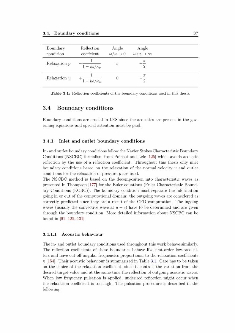
3.4 Boundary conditions
Boundary conditions are crucial in LES since the acoustics are present in the gov-erning equations and special attention must be paid.
3.4.1 Inlet and outlet boundary conditions
In- and outlet boundary conditions follow the Navier Stokes Characteristic BoundaryConditions (NSCBC) formalism from Poinsot and Lele [125] which avoids acousticreflection by the use of a reflection coefficient. Throughout this thesis only inletboundary conditions based on the relaxation of the normal velocity u and outletconditions for the relaxation of pressure p are used.The NSCBC method is based on the decomposition into characteristic waves aspresented in Thompson [177] for the Euler equations (Euler Characteristic Bound-ary Conditions (ECBC)). The boundary condition must separate the informationgoing in or out of the computational domain: the outgoing waves are considered ascorrectly predicted since they are a result of the CFD computation. The ingoingwaves (usually the convective wave at u − c) have to be determined and are giventhrough the boundary condition. More detailed information about NSCBC can befound in [91, 125, 131].
3.4.1.1 Acoustic behaviour
The in- and outlet boundary conditions used throughout this work behave similarly.The reflection coefficients of these boundaries behave like first-order low-pass fil-ters and have cut-off angular frequencies proportional to the relaxation coefficientsκ [154]. Their acoustic behaviour is summarized in Table 3.1. Care has to be takenon the choice of the relaxation coefficient, since it controls the variation from thedesired target value and at the same time the reflection of outgoing acoustic waves.When low frequency pulsation is applied, undesired reflection might occur whenthe relaxation coefficient is too high. The pulsation procedure is described in thefollowing.
38 Chapter 3. Numerical method
3.4.1.2 Pulsation procedure
Forcing is introduced by using the inlet wave modulation method [78]. This methodallows accurate predictions of FTF because only the amplitude of the ingoing acous-tic wave is forced. Forcing the inlet velocity would lead to excitation of eigenmodesin the burner preventing the correct prediction of FTF [78]. Two types of excitationsignals are used in this thesis: a harmonic and a broadband excitation which willbe described in more details in section 3.5.1.
3.4.2 Wall treatment
On solid walls wall-law formulation are used [16, 62, 163]. The normal velocitycomponent with respect to the wall normal is set to zero, while the no-slip conditionis relaxed to allow for a non-null velocity component parallel to the walls. Today,resolving the boundary layer in the context of LES for industrial applications isbeyond the computational resources available [122] and the fluid friction on solidwalls is therefore modeled with a law of the wall boundary condition. The walls ofall configuration throughout this work are modeled following a wall law conditionwith either adiabatic treatment or combined with a heat flux through the wall [145].
3.4.2.1 Adiabatic wall law
The dimensionless variables for the wall-distance and the velocity in the boundarylayer are defined as
y+ =ywuτνw
(3.30)
andu+ =
u2
uτ(3.31)
with yw being the cell height perpendicular to the wall, the mean velocity u2 andthe viscosity on the wall νw. The wall shear stress is τw = ρu2
τ . The friction velocityuτ follows either a linear relation u+ = y+ (for y+ ≤ 11.445) or the logarithmic lawof the wall y+ = C−1ln(Ey+) (for y+ > 11.445, with C = 0.41 and E = 9.2).
3.4.2.2 Heat flux wall law
Heat losses through the wall are crucial for the occurrence of thermo-acoustic insta-bilities since they can have an effect on the stabilization of the flame [156, 176]. Asimple dual model is used for modeling the heat loss through the wall and followsthe linear law
qw =Tref − Tw
Rw(3.32)
where qw describes the heat flux at the wall, Tref an outside reference temperature,Tw the wall temperature and Rw the total heat resistance of wall conduction andconvection outside the chamber. The heat resistance is Rw = e
λ + 1h with the

3.5. LES and System identification 39
material thickness e and the heat resistance e/λ and 1/h of the conduction throughthe chamber wall and outside convection respectively (Fig. 3.3). Convection from
Figure 3.3: Typical velocity profile near the wall and notation used for near-wall quanti-ties [145].
the fluid to the wall is modeled by the logarithmic law of the wall as:
T+ =ρwCp,wuτ (Tw − T2)
qw(3.33)
The heat wall flux qw follows (like uτ ) either a linear relation T+ = Pry+ (for y+ ≤11.445) or the logarithmic law of the wall T+ = C−1Prtln(Fy+) (for y+ > 11.445,with C = 0.41 and F = 2.96).
3.5 LES and System identification
System identification is a crucial step in LES in order to determine the FTF correctly.The process used here, follows the methods utilized and tested by TU Munich [43,50, 64–66, 128] and are summarized in the following.
3.5.1 Excitation signal
Throughout this work, two different types of excitation signals are chosen:
• Harmonic excitation:A sinusoidal perturbation is introduced and one obtains the flame response inone LES for each frequency so that several simulations are needed to cover thefrequency range. The harmonic excitation signal follows:
u(t) = u0sin(ωt) (3.34)
40 Chapter 3. Numerical method
Postprocessing is performed with a Fast Fourier Transformation (section 3.5.2.1)of the velocity and heat release signals.
• Broadband excitation:This method allows the determination of the whole FTF in one single LES.Several broadband signals can be found in literature, as e.g. white noise, sinusoverlay or a discrete random binary signal (DBRS). White noise is a pseudo-random signal distributed uniformly between 0 and 1 and the sinus overlay isgenerated by a superposition of sine waves. In this study a DBRS signal ischosen, which is a discrete random binary signal taking only two values +u0
and −u0. It is given through:
u(t) = u0sign(rand(m)− 0.5) (3.35)
where "sign" is the sign function taking the value 1 or −1 depending on thesign of the randomly generated number m which is between 0 and 1. DBRS ischosen as excitation signal because it has compared to the others the lowestcrest factor [64–66]. The crest factor has been proposed by Ljung [105] and isdefined as:
Cr =
√maxn(x2
n)
1/N∑N
n=1 x2n
(3.36)
It is equal to the peak amplitude of the waveform divided by the mean squareof the zero mean signal allowing to judge the maximal amplitude distributionover a wide range of frequencies. A good signal waveform corresponds (follow-ing Ljung) to a small crest factor.
In order to avoid reflection on the NSCBC boundary conditions (cf. sec-tion 3.4.1) in the low frequency range, the DBRS signal is high-pass filtered.Furthermore it is low-pass filtered to excite only the frequency range of inter-est and to achieve a higher power spectrum density [64–66].
The FTF identification is performed with the Wiener Hopf method, whichis presented in the next section.
3.5.2 System identification
The identification process must give the flame transfer function of an unknown con-figuration [43, 50, 64–66, 128]. Therefore the system is considered as a "black box"only knowing the input signal s(t) and the system response r(t) as illustrated inFig. 3.4. For the FTF, the velocity just upstream of the flame is considered as inputand the global heat release rate as output signal.
According to system identification theory [105], a linear time-invariant (LTI), causalsystem with an input signal s and a output response r at time t can be described
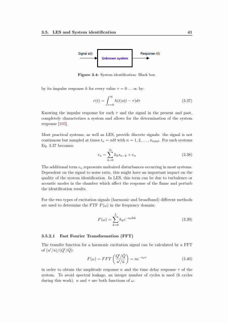
3.5. LES and System identification 41
Figure 3.4: System identification: Black box.
by its impulse response h for every value τ = 0 . . .∞ by:
r(t) =
∫ ∞τ=0
h(t)s(t− τ)dτ (3.37)
Knowing the impulse response for each τ and the signal in the present and past,completely characterizes a system and allows for the determination of the systemresponse [105].
Most practical systems, as well as LES, provide discrete signals: the signal is notcontinuous but sampled at times tn = nδt with n = 1, 2, . . . , ntotal. For such systemsEq. 3.37 becomes:
rn =
∞∑k=0
hksn−k + en (3.38)
The additional term en represents undesired disturbances occurring in most systems.Dependent on the signal to noise ratio, this might have an important impact on thequality of the system identification. In LES, this term can be due to turbulence oracoustic modes in the chamber which affect the response of the flame and perturbthe identification results.
For the two types of excitation signals (harmonic and broadband) different methodsare used to determine the FTF F (ω) in the frequency domain:
F (ω) =
L∑k=0
hke−iωδtk (3.39)
3.5.2.1 Fast Fourier Transformation (FFT)
The transfer function for a harmonic excitation signal can be calculated by a FFTof (u′/u)/(Q′/Q):
F (ω) = FFT
(Q′/Q
u′/u
)= ne−iωτ (3.40)
in order to obtain the amplitude response n and the time delay response τ of thesystem. To avoid spectral leakage, an integer number of cycles is used (6 cyclesduring this work). n and τ are both functions of ω.

42 Chapter 3. Numerical method
3.5.2.2 Wiener Hopf Inversion (WHI)
The Wiener Hopf inversion is a method to reconstruct the transfer function betweena signal and a response for a broadband excitation. This allows for the FTF de-termination over the whole frequency range with only one simulation. It has firstbeen introduced to the CFD community by Polifke et al. [129] and Gentemann etal. [50]. The underlaying theory is briefly described here. Detailed information isgiven in [65, 66, 129].
For a broadband excitation it is difficult to separate which contributions of theflame response are due to the excitation signal and due to undesired disturbancesrepresented by an error en in Eq. 3.38. The Wiener Hopf transformation minimizesen in a least-mean squared sense [105] and writes
Γh = c (3.41)
where Γ is the auto-correlation matrix of the input signals
Γij =1
N − L+ 1
N∑k=L
sk−isk−j for i, j = 0, . . . , L (3.42)
and c the cross-correlation vector of the input signals and the responses
cij =1
N − L+ 1
N∑k=L
sk−irk for i, j = 0, . . . , L (3.43)
N denotes the number of considered time steps and L corresponds to the filter"memory". L has to account for the longest time lag of the system in order tocapture all relevant physical effects [49]. In combustion instabilities this is usuallythe convective time scale [129]. The memory of the filter τMEM is given throughτMEM = (L− 1)δt.
The so-called Wiener-Hopf Inversion
h = Γ−1c (3.44)
and a subsequent z-transformation allow finally to determine the transfer functionof the system. The identification procedure is illustrated in Fig. 3.5. The validfrequency range for the transfer function is determined by the time step δt throughthe Nyquist criterion fmax = 1/(2δt) and the length of the time series (e.g. thesimulation time) T = ntotalδt from fmin = 1/T .
The time step in LES is generally very small and a large filter length L wouldbe needed in order to capture the longest time lag of the system. This leads to ahigh order of the auto-correlation matrix Γij and to errors in the system identifica-tion during inversion due to bad conditioning [49]. In order to reduce the size of Γ

3.5. LES and System identification 43
Figure 3.5: System identification process with Wiener-Hopf (adapted from [176]).
a factor m is introduced so that the auto-correlation matrix now writes:
Γij =1
N − Lm+ 1
N∑k=Lm
sk−misk−mj for i, j = 0, . . . , L (3.45)
The cross-correlation vector is in this case
cij =1
N − Lm+ 1
N∑k=Lm
sk−mirk for i, j = 0, . . . , L (3.46)
Of course, the valid frequency range for the identification procedure changes tofmax = 1/(2mδt). A detailed analysis of this method can be found in [49].

Part III
Application to a perfectlypremixed swirler combustor: the
FVV burner

Chapter 4
Target configuration
Contents4.1 The FVV test rig . . . . . . . . . . . . . . . . . . . . . . . . . 47
4.1.1 Experimental set-up . . . . . . . . . . . . . . . . . . . . . . . 484.1.2 Operating point . . . . . . . . . . . . . . . . . . . . . . . . . 49
4.2 Description of the numerical setup . . . . . . . . . . . . . . . 494.2.1 Computational mesh . . . . . . . . . . . . . . . . . . . . . . . 504.2.2 Boundary conditions . . . . . . . . . . . . . . . . . . . . . . . 514.2.3 Numerical parameters . . . . . . . . . . . . . . . . . . . . . . 51
The aim of this part is to validate the modeling for a lean premixed swirledburner at atmospheric pressure featuring a highly turbulent flow (Re ≈ 35000) butalso to estimate the uncertainties associated to a given LES approach to computemean flows and FTFs in a swirled burner (FVV burner). Therefore the LES codeAVBP is compared against experiments (performed at TU Berlin [142–144]) and tovalidate the modeling independently of the code used, against OpenFoam [1] LESsimulations (performed at Siemens [89]). Thanks to the detailed data made avail-able by LES, mechanisms can be identified influencing the dynamic behaviour ofthe flame.
This part is organized as follows: chapter 4 describes the FVV test rig, the operat-ing point and the experiments used to characterize the flame and flow field. Then(section 4.2) the simulation domain, mesh, boundary conditions and numerical pa-rameters are specified. Chapter 5 discusses the numerical results and validates themagainst experiments and the LES code OpenFoam (section 5.1.2). Furthermore theacoustically perturbed flame is analyzed and the FTF is validated in section 5.2.2.Finally the impact of different mechanisms influencing the dynamic flame responseis analyzed (section 5.2.3).
4.1 The FVV test rig
The experimental test rig is located at the University of Berlin and operates underatmospheric conditions. All experimental results shown here have been providedby Schimek et al. [89, 142–144] who studied the swirl-stabilized premixed flameextensively. Figure 4.1 illustrates the experimental configuration. Preheated air

48 Chapter 4. Target configuration
Figure 4.1: Experimental test rig [143]
passes the upstream duct, enters the swirl generator and reaches the combustionchamber through an annular duct. The flame is stabilized through an inner andouter recirculation zone resulting from the vortex breakdown due to the suddengeometrical expansion. The main parameters of the test rig are summarized intable 4.1. The upstream duct is variable in length in order to generate resonance in
Upstream duct Length 2.0 to 2.7 mDiameter 0.1484 m
Annular duct Length 0.171 mDiameter interior 0.0275 mDiameter exterior 0.055 m
Combustion chamber Length 1.5 mDiameter 0.2 m
Table 4.1: Main parameters of the FVV configuration.
the combustion chamber when forcing is applied by the four loudspeakers mountedat the duct inlet (Fig. 4.1). The lowest resonance frequency is around 50 Hz andthe second around 100 Hz with no resonance in between, whereas above 100 Hzmultiple higher frequency modes appear. An acoustic forcing of up to 100 % of themean velocity in the annular duct can be reached in order to meet desired excitationamplitudes at a given frequency. The swirl generator possesses movable blocks toapply for a wide range of swirl numbers from 0 up to approx. 2 (Fig. 4.2).
4.1.1 Experimental set-up
The acoustics of the duct are characterized via the multi microphone method, andthe velocity fluctuation in the annular duct is obtained through reconstruction of

4.2. Description of the numerical setup 49
Figure 4.2: Cross-section of swirler, annular duct and combustion chamber [142].
the transfer matrix of the swirl generator. Fluctuations of heat release rate aremeasured with OH* chemiluminescence. Measurements are available for a varietyof operating conditions including technically premixed (air and fuel are injected sep-arately and mixed prior to combustion) and perfectly premixed operation, variationin swirl number, mass flow rates and equivalence ratios. In the technically premixedcase, fuel is injected through sixteen holes in the swirl generator whereas for theperfectly premixed operating point, fuel and air is mixed far upstream of the swirler(Fig. 4.2). The reader is referred to [142, 143] for further information.
4.1.2 Operating point
This part focusses on the perfectly premixed operating conditions where fuel andair are mixed far upstream and a fully premixed mixture reaches the combustionchamber. This operating point is detailed in Table 4.2. The goal is to validate theLES methodology used against experimental mean flow fields and the flame transferfunction and furthermore to obtain insight into the saturation mechanisms of theFTF amplitude.
4.2 Description of the numerical setup
This section presents first the computational mesh for the LES and the boundaryconditions are given. The pulsation procedure for FTF determination is shortly de-scribed and finally the numerical parameters used for the calculation are explained.
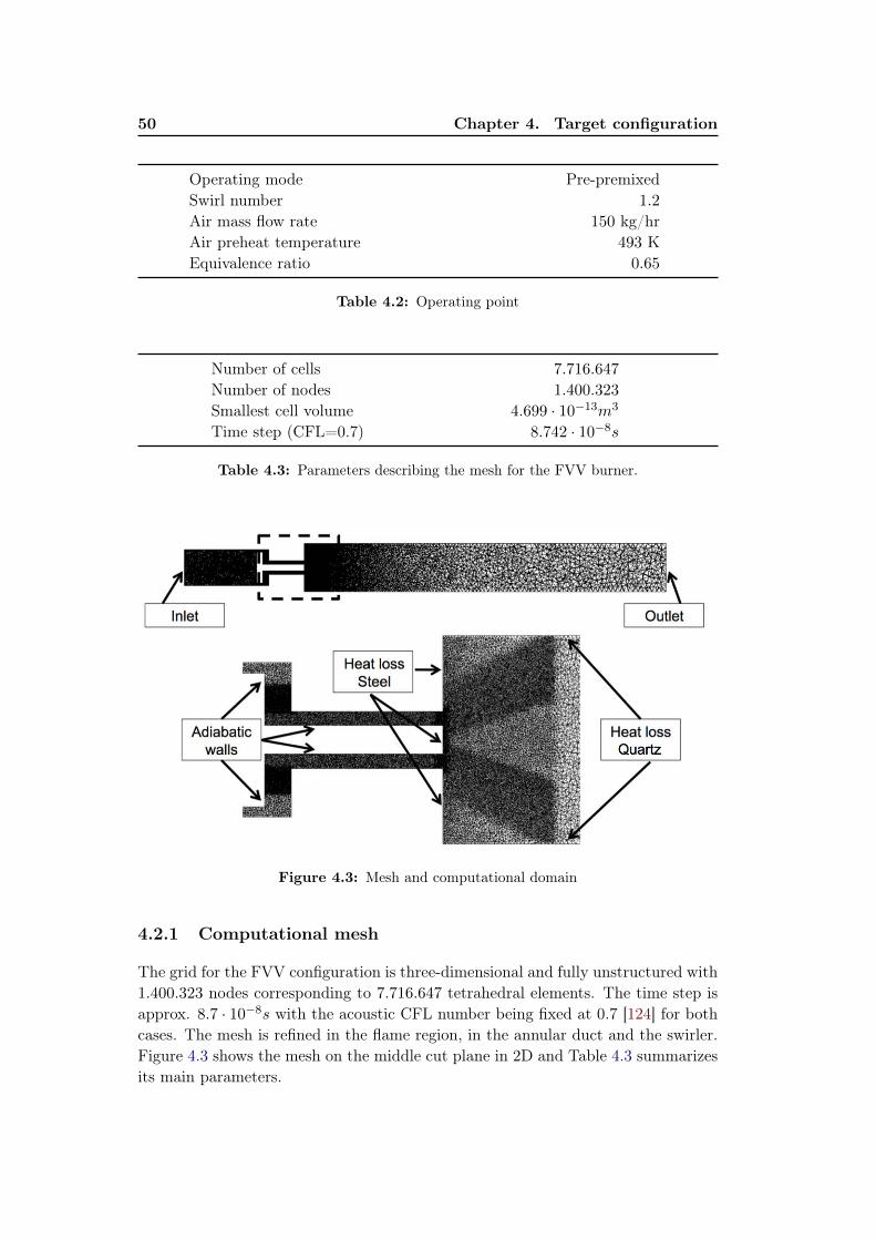
50 Chapter 4. Target configuration
Operating mode Pre-premixedSwirl number 1.2
Air mass flow rate 150 kg/hrAir preheat temperature 493 KEquivalence ratio 0.65
Table 4.2: Operating point
Number of cells 7.716.647
Number of nodes 1.400.323
Smallest cell volume 4.699 · 10−13m3
Time step (CFL=0.7) 8.742 · 10−8s
Table 4.3: Parameters describing the mesh for the FVV burner.
Figure 4.3: Mesh and computational domain
4.2.1 Computational mesh
The grid for the FVV configuration is three-dimensional and fully unstructured with1.400.323 nodes corresponding to 7.716.647 tetrahedral elements. The time step isapprox. 8.7 · 10−8s with the acoustic CFL number being fixed at 0.7 [124] for bothcases. The mesh is refined in the flame region, in the annular duct and the swirler.Figure 4.3 shows the mesh on the middle cut plane in 2D and Table 4.3 summarizesits main parameters.
4.2. Description of the numerical setup 51
4.2.2 Boundary conditions
The inlet and outlet boundary conditions are imposed through the non-reflectingNavier-Stokes Characteristic Boundary Condition (NSCBC) formulation [125] whichlimits acoustic reflection. For the combustion chamber walls a logarithmic wall-lawcondition is set and additionally applies for heat loss effects since it is essential forflame stabilization and thus the correct prediction of FTF [176]. The model for heatloss through the wall follows the linear law presented in section 3.4.1:
qwall =Tref − Twall
Rwall(4.1)
where qwall describes the heat flux at the wall, Tref a reference temperature, Twallthe wall temperature and Rwall the combined heat resistance of conduction throughthe material and outside convection. The side walls of the combustion chamber aremade out of quarzglas with a thickness of 6 mm resulting in a heat resistance of1/Rwall = 500W/m2K if the outside convection coefficient h is large. The end wallsof the combustor, i.e. where the flame stabilizes, consist of steel 1.4301 with a thick-ness of 8 mm which results in 1/Rwall = 1875W/m2K. The reference temperatureis set to 300 K. All other walls follow an adiabatic wall-law.Flame transfer functions are determined via pure tone excitation for different fre-quencies. Therefore an harmonic perturbation is introduced through the inlet usingthe inlet wave modulation method [78] and the perturbation of the total heat releaserate is measured.
4.2.3 Numerical parameters
The fully compressible explicit code AVBP is used to solve the reactive multi-speciesNavier-Stokes equations on unstructured grids using a cell-vertex approximation[147]. A second order finite element scheme is used for both time and space advance-ment [57, 94]. Sub-grid stress tensor is modeled by a classical Smagorinsky approach[161]. Chemistry is computed using a two step mechanism for Methane/Air flames[44–46] where the full chemistry is replaced by two reactions taking into account sixspecies (CH4, O2, CO2, CO, H2O and N2):
CH4 +3
2O2 −→ CO + 2H2O (4.2)
CO +1
2O2 ←→ CO2 (4.3)
The first reaction is irreversible and decribes the rate of reaction as follows:
q1 = A1
(ρYCH4
WCH4
)nCH41
(ρYO2
WO2
)nO21
exp
(−Ea1
RT
)(4.4)
The second reaction is reversible and leads to an equilibrium between CO and CO2
in the burnt gases. Its rate of reaction is given through:
q2 = A2
(ρYCOWCO
)nCO2(ρYO2
WO2
)nO22(ρYCO2
WCO2
)nCO22
exp(−Ea2
RT
)(4.5)

52 Chapter 4. Target configuration
Numerical scheme Lax-WendroffSub-grid scale model Smagorinsky modelArtificial viscosity model Colin Sensor (ε2 = 0.05; ε4 = 0.01)Chemistry Two-step BFERFlame/turbulence interaction Thickened flame model
Table 4.4: Numerical parameters used for the FVV simulation.
A1 Ea1 nCH41 nO2
1
4.9 · 109cgs 35500cal/mol 0.5 0.65
A2 Ea2 nCO2 nO22 nCO2
2
−2.0 · 108cgs 12000cal/mol 1.0 0.5 0.0
Table 4.5: Coefficients used in the reduced chemical scheme for CH4/air flames.
This scheme was developed and fitted to match the full mechanism’s behaviour forequivalence ratios between 0.4 and 1.5 [45, 46]. To capture flame/turbulence in-teractions, the dynamic thickened flame model is used. The flame sub-grid-scalewrinkling and interactions are supplied by an efficiency function [25, 27, 98]. Thenumerical parameters are summarized in Table 4.4 and the coefficients for the re-duced chemical scheme can be found in Table 4.5.
Chapter 5
LES of the reacting unforced andforced flows in the FVV setup
Contents5.1 Reacting flow fields . . . . . . . . . . . . . . . . . . . . . . . . 53
5.1.1 Mean reacting flow fields with AVBP . . . . . . . . . . . . . . 53
5.1.2 Comparison Between AVBP, Openfoam and PIV . . . . . . . 56
5.2 Forced reacting flow . . . . . . . . . . . . . . . . . . . . . . . . 60
5.2.1 Pulsation procedure . . . . . . . . . . . . . . . . . . . . . . . 60
5.2.2 Flame Transfer Function . . . . . . . . . . . . . . . . . . . . . 60
5.2.3 Mechanisms affecting the FTF . . . . . . . . . . . . . . . . . 61
5.3 Conclusions . . . . . . . . . . . . . . . . . . . . . . . . . . . . . 63
5.1 Reacting flow fields
The following section describes first the averaged and instantaneous flow field ob-tained with AVBP for the turbulent unforced cases. In the second section a com-parison of simulation results obtained with AVBP and OpenFoam at different axialcuts in the combustion chamber is performed and compared to PIV measurementsobtained by TU Berlin. The reader is referred to [142–144] and [89] for detailed in-formation about the PIV measurements and the OpenFoam simulation respectively.
5.1.1 Mean reacting flow fields with AVBP
A first impression of the flow field can be obtained by plotting the instantaneousaxial velocity field in the middle cut plane and a three-dimensional iso-surface ofthe flame (T = 1200 K) in Fig. 5.1. A highly turbulent flow develops in the annularflame tube and a wrinkled flame is stabilized by the inner and outer recirculationzones resulting from the vortex breakdown and the sudden expansion. The averagedaxial velocity field (Fig. 5.2) shows that the flow is accelerated at the chamber inletand that a large inner recirculation zone and strong outer recirculation zones areformed. The velocity at the outlet of the annular flame tube is higher at the outer
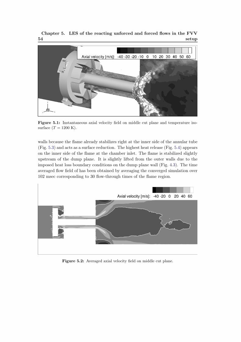
54Chapter 5. LES of the reacting unforced and forced flows in the FVV
setup
Figure 5.1: Instantaneous axial velocity field on middle cut plane and temperature iso-surface (T = 1200 K).
walls because the flame already stabilizes right at the inner side of the annular tube(Fig. 5.3) and acts as a surface reduction. The highest heat release (Fig. 5.4) appearson the inner side of the flame at the chamber inlet. The flame is stabilized slightlyupstream of the dump plane. It is slightly lifted from the outer walls due to theimposed heat loss boundary conditions on the dump plane wall (Fig. 4.3). The timeaveraged flow field of has been obtained by averaging the converged simulation over102 msec corresponding to 30 flow-through times of the flame region.
Figure 5.2: Averaged axial velocity field on middle cut plane.
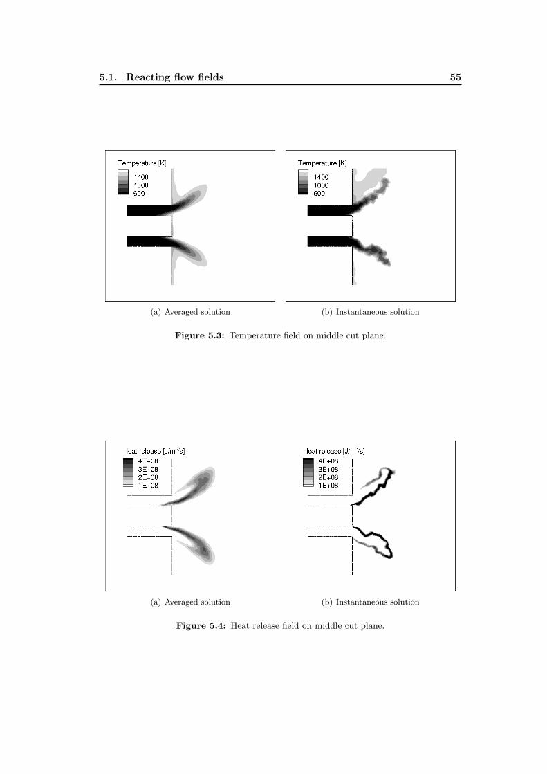
5.1. Reacting flow fields 55
(a) Averaged solution (b) Instantaneous solution
Figure 5.3: Temperature field on middle cut plane.
(a) Averaged solution (b) Instantaneous solution
Figure 5.4: Heat release field on middle cut plane.

56Chapter 5. LES of the reacting unforced and forced flows in the FVV
setup
5.1.2 Comparison Between AVBP, Openfoam and PIV
Particle image velocimetry experiments and averaged results are compared here tothe LES computations performed with AVBP and OpenFoam. Figure 5.6 illustratesthe mean temperature field for both codes at position x = 0.01, 0.02, 0.03, 0.04, 0.05
and 0.1 m from the combustion chamber entrance corresponding to x = 0 as illus-trated in Fig. 5.5.
AVBP and Openfoam show good overall agreement. The maximal temperatures inthe chamber predicted by the two solvers agree although a different approach is usedwith OpenFoam: i.e. iso-thermal wall conditions against a heat flux through thewall with AVBP. These differences partly explain the different temperatures directlyat the wall. Axial velocity profiles are compared with PIV data in Fig. 5.7. Theinner recirculation zone is well represented by both codes. The outer recirculationzone is over predicted. The results of AVBP are slightly closer to the measurementscompared to OpenFoam but both codes overestimate the recirculated flow rate.
The radial and tangential velocity profiles (Fig. 5.8 and 5.9) reproduce well thelocation and magnitude of extrema for the inner recirculation zone. Room for im-provement is still present compared to experiments for the outer recirculation zone.Again, the simulation with AVBP is slightly closer to PIV. Note that following [89],measurement errors might be present due to window contamination in this region.Considering that both LES codes agree very well away from these regions, errors inPIV measurements are possible.
Although temperature and velocity profiles agree well, differences between AVBPand OpenFoam are observed for the RMS fluctuations. RMS temperature pro-files (Fig. 5.10) are similar at the chamber inlet, but almost double in AVBP at
Figure 5.5: Reference plane for FTF determination, location of cuts at ∆x =
0.01, 0.02, 0.03, 0.04, 0.05 and 0.1 m and iso-line of temperature (T = 1200 K).
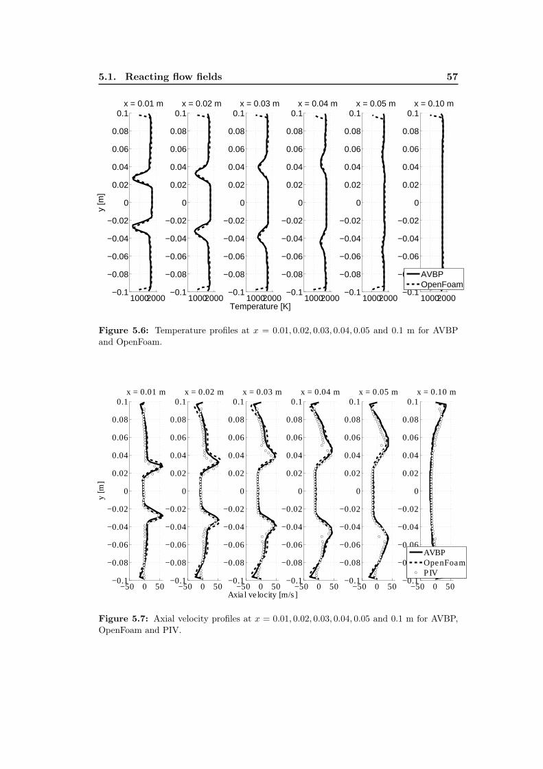
5.1. Reacting flow fields 57
10002000−0.1
−0.08
−0.06
−0.04
−0.02
0
0.02
0.04
0.06
0.08
0.1
y [
m]
x = 0.01 m
10002000−0.1
−0.08
−0.06
−0.04
−0.02
0
0.02
0.04
0.06
0.08
0.1x = 0.02 m
10002000−0.1
−0.08
−0.06
−0.04
−0.02
0
0.02
0.04
0.06
0.08
0.1
Temperature [K]
x = 0.03 m
10002000−0.1
−0.08
−0.06
−0.04
−0.02
0
0.02
0.04
0.06
0.08
0.1x = 0.04 m
10002000−0.1
−0.08
−0.06
−0.04
−0.02
0
0.02
0.04
0.06
0.08
0.1x = 0.05 m
10002000−0.1
−0.08
−0.06
−0.04
−0.02
0
0.02
0.04
0.06
0.08
0.1x = 0.10 m
AVBP
OpenFoam
Figure 5.6: Temperature profiles at x = 0.01, 0.02, 0.03, 0.04, 0.05 and 0.1 m for AVBPand OpenFoam.
−50 0 50−0.1
−0.08
−0.06
−0.04
−0.02
0
0.02
0.04
0.06
0.08
0.1
y [
m]
x = 0.01 m
−50 0 50−0.1
−0.08
−0.06
−0.04
−0.02
0
0.02
0.04
0.06
0.08
0.1x = 0.02 m
−50 0 50−0.1
−0.08
−0.06
−0.04
−0.02
0
0.02
0.04
0.06
0.08
0.1
Axial velocity [m/s]
x = 0.03 m
−50 0 50−0.1
−0.08
−0.06
−0.04
−0.02
0
0.02
0.04
0.06
0.08
0.1x = 0.04 m
−50 0 50−0.1
−0.08
−0.06
−0.04
−0.02
0
0.02
0.04
0.06
0.08
0.1x = 0.05 m
−50 0 50−0.1
−0.08
−0.06
−0.04
−0.02
0
0.02
0.04
0.06
0.08
0.1x = 0.10 m
AVBP
OpenFoam
PIV
Figure 5.7: Axial velocity profiles at x = 0.01, 0.02, 0.03, 0.04, 0.05 and 0.1 m for AVBP,OpenFoam and PIV.
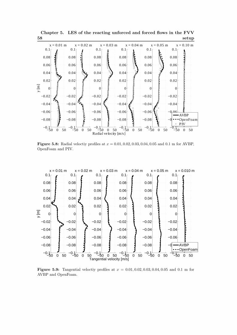
58Chapter 5. LES of the reacting unforced and forced flows in the FVV
setup
−50 0 50−0.1
−0.08
−0.06
−0.04
−0.02
0
0.02
0.04
0.06
0.08
0.1
y [
m]
x = 0.01 m
−50 0 50−0.1
−0.08
−0.06
−0.04
−0.02
0
0.02
0.04
0.06
0.08
0.1x = 0.02 m
−50 0 50−0.1
−0.08
−0.06
−0.04
−0.02
0
0.02
0.04
0.06
0.08
0.1
Radial velocity [m/s]
x = 0.03 m
−50 0 50−0.1
−0.08
−0.06
−0.04
−0.02
0
0.02
0.04
0.06
0.08
0.1x = 0.04 m
−50 0 50−0.1
−0.08
−0.06
−0.04
−0.02
0
0.02
0.04
0.06
0.08
0.1x = 0.05 m
−50 0 50−0.1
−0.08
−0.06
−0.04
−0.02
0
0.02
0.04
0.06
0.08
0.1x = 0.10 m
AVBP
OpenFoam
PIV
Figure 5.8: Radial veloctiy profiles at x = 0.01, 0.02, 0.03, 0.04, 0.05 and 0.1 m for AVBP,OpenFoam and PIV.
−50 0 50−0.1
−0.08
−0.06
−0.04
−0.02
0
0.02
0.04
0.06
0.08
0.1
y [
m]
x = 0.01 m
−50 0 50−0.1
−0.08
−0.06
−0.04
−0.02
0
0.02
0.04
0.06
0.08
0.1x = 0.02 m
−50 0 50−0.1
−0.08
−0.06
−0.04
−0.02
0
0.02
0.04
0.06
0.08
0.1
Tangential velocity [m/s]
x = 0.03 m
−50 0 50−0.1
−0.08
−0.06
−0.04
−0.02
0
0.02
0.04
0.06
0.08
0.1x = 0.04 m
−50 0 50−0.1
−0.08
−0.06
−0.04
−0.02
0
0.02
0.04
0.06
0.08
0.1x = 0.05 m
−50 0 50−0.1
−0.08
−0.06
−0.04
−0.02
0
0.02
0.04
0.06
0.08
0.1x = 0.010 m
AVBP
OpenFoam
Figure 5.9: Tangential veloctiy profiles at x = 0.01, 0.02, 0.03, 0.04, 0.05 and 0.1 m forAVBP and OpenFoam.

5.1. Reacting flow fields 59
x = 0.04m. Since no PIV data is available, it is difficult to conclude here thatAVBP is better. However, the smaller RMS values obtained with OpenFoam areconsistent with the larger dissipation observed in this solver.
0 500−0.1
−0.08
−0.06
−0.04
−0.02
0
0.02
0.04
0.06
0.08
0.1
y [
m]
x = 0.01 m
0 500−0.1
−0.08
−0.06
−0.04
−0.02
0
0.02
0.04
0.06
0.08
0.1x = 0.02 m
0 500−0.1
−0.08
−0.06
−0.04
−0.02
0
0.02
0.04
0.06
0.08
0.1
Trms
[K]
x = 0.03 m
0 500−0.1
−0.08
−0.06
−0.04
−0.02
0
0.02
0.04
0.06
0.08
0.1x = 0.04 m
0 500−0.1
−0.08
−0.06
−0.04
−0.02
0
0.02
0.04
0.06
0.08
0.1x = 0.05 m
0 500−0.1
−0.08
−0.06
−0.04
−0.02
0
0.02
0.04
0.06
0.08
0.1x = 0.10 m
AVBP
OpenFoam
Figure 5.10: RMS temperature profiles at x = 0.01, 0.02, 0.03, 0.04, 0.05 and 0.1 m forAVBP and OpenFoam.
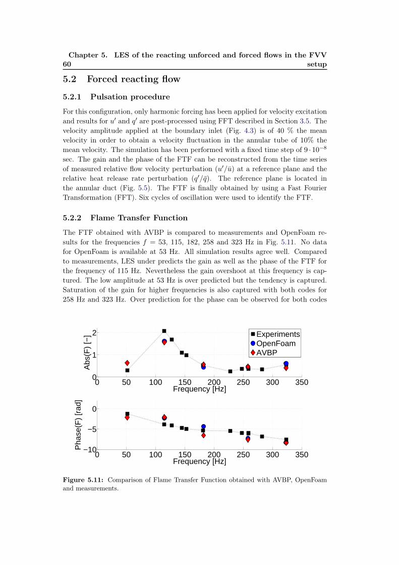
60Chapter 5. LES of the reacting unforced and forced flows in the FVV
setup
5.2 Forced reacting flow
5.2.1 Pulsation procedure
For this configuration, only harmonic forcing has been applied for velocity excitationand results for u′ and q′ are post-processed using FFT described in Section 3.5. Thevelocity amplitude applied at the boundary inlet (Fig. 4.3) is of 40 % the meanvelocity in order to obtain a velocity fluctuation in the annular tube of 10% themean velocity. The simulation has been performed with a fixed time step of 9 · 10−8
sec. The gain and the phase of the FTF can be reconstructed from the time seriesof measured relative flow velocity perturbation (u′/u) at a reference plane and therelative heat release rate perturbation (q′/q). The reference plane is located inthe annular duct (Fig. 5.5). The FTF is finally obtained by using a Fast FourierTransformation (FFT). Six cycles of oscillation were used to identify the FTF.
5.2.2 Flame Transfer Function
The FTF obtained with AVBP is compared to measurements and OpenFoam re-sults for the frequencies f = 53, 115, 182, 258 and 323 Hz in Fig. 5.11. No datafor OpenFoam is available at 53 Hz. All simulation results agree well. Comparedto measurements, LES under predicts the gain as well as the phase of the FTF forthe frequency of 115 Hz. Nevertheless the gain overshoot at this frequency is cap-tured. The low amplitude at 53 Hz is over predicted but the tendency is captured.Saturation of the gain for higher frequencies is also captured with both codes for258 Hz and 323 Hz. Over prediction for the phase can be observed for both codes
0 50 100 150 200 250 300 3500
1
2
Frequency [Hz]
Abs(F
) [−
]
ExperimentsOpenFoamAVBP
0 50 100 150 200 250 300 350−10
−5
0
Frequency [Hz]
Phase(F
) [r
ad]
Figure 5.11: Comparison of Flame Transfer Function obtained with AVBP, OpenFoamand measurements.
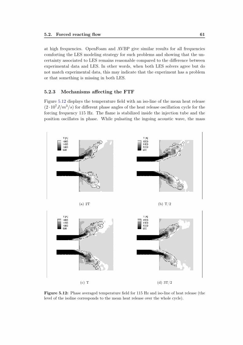
5.2. Forced reacting flow 61
at high frequencies. OpenFoam and AVBP give similar results for all frequenciescomforting the LES modeling strategy for such problems and showing that the un-certainty associated to LES remains reasonable compared to the difference betweenexperimental data and LES. In other words, when both LES solvers agree but donot match experimental data, this may indicate that the experiment has a problemor that something is missing in both LES.
5.2.3 Mechanisms affecting the FTF
Figure 5.12 displays the temperature field with an iso-line of the mean heat release(2 · 107J/m3/s) for different phase angles of the heat release oscillation cycle for theforcing frequency 115 Hz. The flame is stabilized inside the injection tube and theposition oscillates in phase. While pulsating the ingoing acoustic wave, the mass
(a) 2T (b) T/2
(c) T (d) 3T/2
Figure 5.12: Phase averaged temperature field for 115 Hz and iso-line of heat release (thelevel of the isoline corresponds to the mean heat release over the whole cycle).

62Chapter 5. LES of the reacting unforced and forced flows in the FVV
setup
flow rate oscillates sinusoidally and the flame reacts to this perturbation after acertain time lag (compare Fig. 5.11).
When acoustic perturbations impinge the swirler, axial and transverse velocityfluctuations are created travelling with the speed of sound and the convective veloc-ity respectively. This leads to a phase difference between both velocity componentsresulting in swirl number fluctuations. This is illustrated in Fig. 5.13. At the trail-ing edge of the swirler vanes (plane 1), the axial uax and azimuthal uθ velocitiesare in phase. Within the passage, since the axial signal is propagating at u + c
while the azimuthal perturbations move at u, the phase at plane 2 between bothcomponents can take any value depending on L. This phase is one of the parameterswhich control swirl variation at the chamber inlet. According to Palies et al. [117]this mechanisms has a strong impact on the flame response. As the vortex break-down changes with the swirl number, the size and position of the recirculation zoneschange and affect thus the flame angle. Palies et al. [117] state that an overshootoccurs when axial and azimuthal velocity are in phase when impinging the flamefront and low amplitude when both components are out of phase.
Figure 5.14 and Figure 5.15 show the relative axial (u′ax/uax) and transversevelocity (v′θ/vθ) components at the reference plane (Fig. 5.5) over the normalizedtime for two cycles of axial velocity fluctuation for the two distinct frequencies 53Hz and 115 Hz. Axial and transverse velocities are almost in phase at 53 Hz andin quadrature at 115 Hz. Here, in phase variations of u′ax and u′θ lead to smallerswirl variations and reduced flame angle fluctuations. At 53 Hz, this leads to asmall value of the gain n (Fig. 5.11). Inversely, at 115 Hz, the swirl variations willbe larger, leading to larger values of n. This result does not support Palies model,suggesting that more complex phenomena (in addition to u′ax and u′θ) determine the
Figure 5.13: Illustration of the creation of swirl number perturbations.
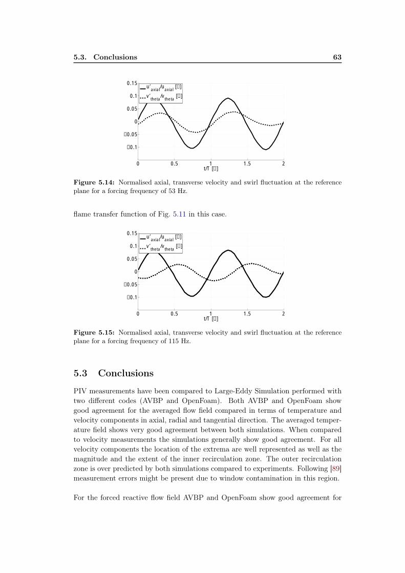
5.3. Conclusions 63
0 0.5 1 1.5 2
−0.1
−0.05
0
0.05
0.1
0.15
t/T [−]
u′axial
/uaxial
[−]
v′theta
/vtheta
[−]
Figure 5.14: Normalised axial, transverse velocity and swirl fluctuation at the referenceplane for a forcing frequency of 53 Hz.
flame transfer function of Fig. 5.11 in this case.
0 0.5 1 1.5 2
−0.1
−0.05
0
0.05
0.1
0.15
t/T [−]
u′axial
/uaxial
[−]
v′theta
/vtheta
[−]
Figure 5.15: Normalised axial, transverse velocity and swirl fluctuation at the referenceplane for a forcing frequency of 115 Hz.
5.3 Conclusions
PIV measurements have been compared to Large-Eddy Simulation performed withtwo different codes (AVBP and OpenFoam). Both AVBP and OpenFoam showgood agreement for the averaged flow field compared in terms of temperature andvelocity components in axial, radial and tangential direction. The averaged temper-ature field shows very good agreement between both simulations. When comparedto velocity measurements the simulations generally show good agreement. For allvelocity components the location of the extrema are well represented as well as themagnitude and the extent of the inner recirculation zone. The outer recirculationzone is over predicted by both simulations compared to experiments. Following [89]measurement errors might be present due to window contamination in this region.
For the forced reactive flow field AVBP and OpenFoam show good agreement for
64Chapter 5. LES of the reacting unforced and forced flows in the FVV
setup
the considered forcing frequencies. The overshoot in gain is predicted as well as thedecreasing gain for higher frequencies. Compared to experiments, the gain at 53 Hzis over predicted and at 115 Hz under predicted while the higher frequencies showbetter agreement. Both codes under predict the phase for 115 Hz and over predictit for the higher frequencies. The general shape however corresponds to the PIVmeasurements.
The flame which is stabilised inside the flame-tube changes its position with theoscillating flow rate. Swirl number fluctuations due to different propagating mech-anisms of axial and azimuthal velocity lead to different FTF amplitude responses.Both velocity components are in quadrature when impinging the flame front leadingto a higher response of the flame at 115 Hz and in phase at 53 Hz where a lowamplitude response occurs. This result does not support Palies model, suggestingthat more complex phenomena determine the flame transfer function amplitude inthis case.
The goal of this part was to validate the modeling for a lean premixed swirled burneragainst experiments and against OpenFoam LES simulations [89]. The LES codeAVBP presented in chapter 3 captures the phenomena appearing during thermo-acoustic instabilities. The next part is dedicated to the simulation of the thermo-acoustic behaviour of a complex real gas turbine application.

Part IV
Application to an industrialcombustor: A Double SwirlerTechnically Premixed Burner

Chapter 6
Target configuration
Contents6.1 Geometries . . . . . . . . . . . . . . . . . . . . . . . . . . . . . 67
6.1.1 Real gas turbine . . . . . . . . . . . . . . . . . . . . . . . . . 686.1.2 Experimental test rig for cold flow validation . . . . . . . . . 70
6.2 Description of the numerical setup . . . . . . . . . . . . . . . 716.2.1 Computational mesh . . . . . . . . . . . . . . . . . . . . . . . 716.2.2 Boundary conditions . . . . . . . . . . . . . . . . . . . . . . . 746.2.3 Numerical parameters . . . . . . . . . . . . . . . . . . . . . . 75
Chapter 1 and 2 in part 1 presented the LES solver and the specificities of annularcombustors. Part 2 validated the LES solver against experiments for a single pre-mixed turbulent swirling flame at atmospheric pressure and identified mechanismsacting on the dynamics of the flame. LES was shown to provide good evaluation ofthe FTF (Flame Transfer Function). The goal of this part is to extend the method-ology to an industrial gas turbine where additional mechanisms come into play whenair and fuel are injected separately and mixing takes place. These mechanisms havebeen studied for simple laboratory flames but much less information is available forreal gas turbines. This point is investigated here for a real burner corresponding toan industrial gas turbine. Thanks to this fully unsteady numerical approach, effectsof mass flow rate perturbation, mixture fluctuation and swirl number perturbationcan be studied.
In the first chapter the configuration will be described and the simulation domain,mesh, boundary conditions and numerical parameters are specified. In chapter 7 thenumerical results will be validated against experiments on an atmospheric test rigand the unforced flame is analyzed in detail for different operating conditions andburner outlets. In chapter 8 acoustic perturbations are introduced and the lineardynamic response of the flames for the different cases is analyzed in detail. Finally,chapter 10 discusses the non-linear flame response to study the flame dynamics whenlimit cycles in real machines occur.
6.1 Geometries
During this work, two configurations have been computed. The first one is a sin-gle sector of the real gas turbine (Section 6.1.1) and the second one is a specific
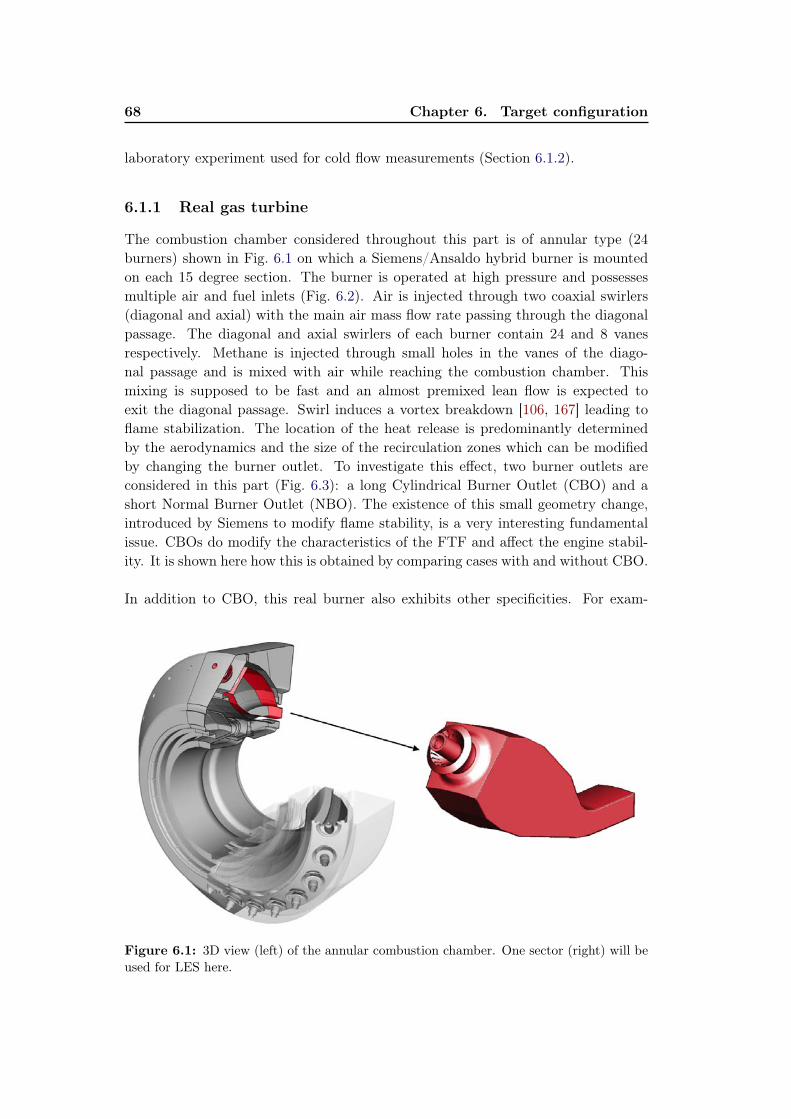
68 Chapter 6. Target configuration
laboratory experiment used for cold flow measurements (Section 6.1.2).
6.1.1 Real gas turbine
The combustion chamber considered throughout this part is of annular type (24burners) shown in Fig. 6.1 on which a Siemens/Ansaldo hybrid burner is mountedon each 15 degree section. The burner is operated at high pressure and possessesmultiple air and fuel inlets (Fig. 6.2). Air is injected through two coaxial swirlers(diagonal and axial) with the main air mass flow rate passing through the diagonalpassage. The diagonal and axial swirlers of each burner contain 24 and 8 vanesrespectively. Methane is injected through small holes in the vanes of the diago-nal passage and is mixed with air while reaching the combustion chamber. Thismixing is supposed to be fast and an almost premixed lean flow is expected toexit the diagonal passage. Swirl induces a vortex breakdown [106, 167] leading toflame stabilization. The location of the heat release is predominantly determinedby the aerodynamics and the size of the recirculation zones which can be modifiedby changing the burner outlet. To investigate this effect, two burner outlets areconsidered in this part (Fig. 6.3): a long Cylindrical Burner Outlet (CBO) and ashort Normal Burner Outlet (NBO). The existence of this small geometry change,introduced by Siemens to modify flame stability, is a very interesting fundamentalissue. CBOs do modify the characteristics of the FTF and affect the engine stabil-ity. It is shown here how this is obtained by comparing cases with and without CBO.
In addition to CBO, this real burner also exhibits other specificities. For exam-
Figure 6.1: 3D view (left) of the annular combustion chamber. One sector (right) will beused for LES here.
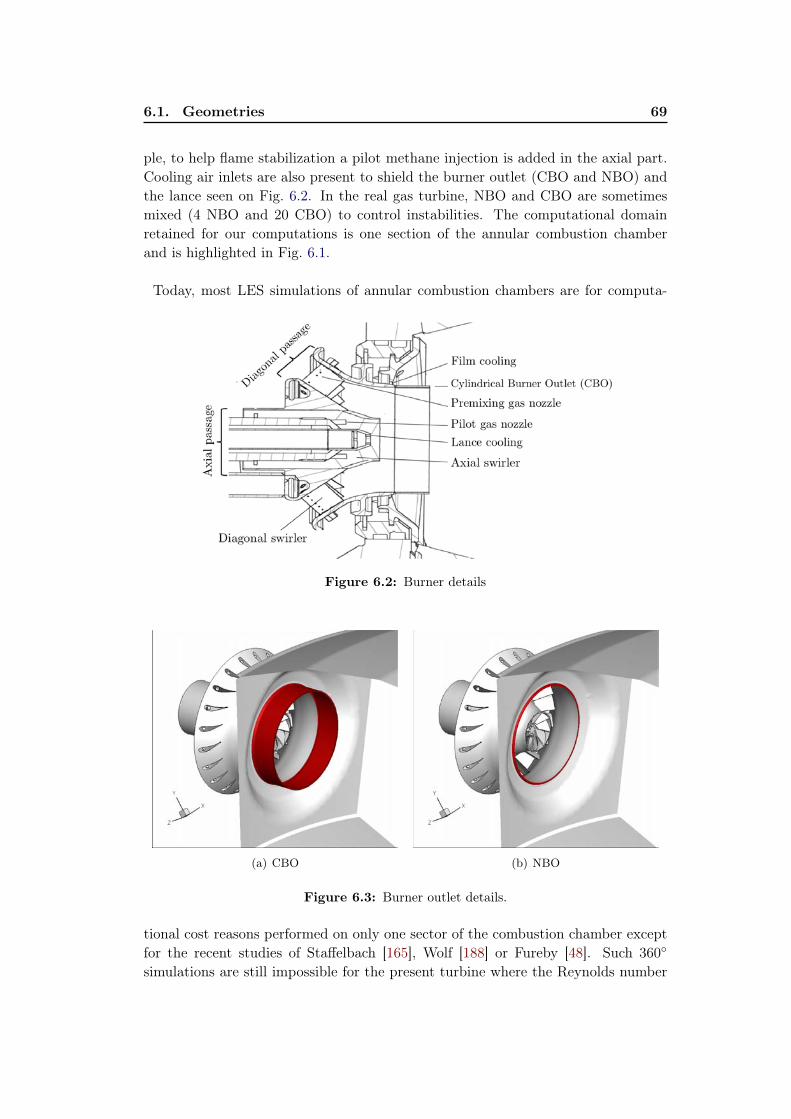
6.1. Geometries 69
ple, to help flame stabilization a pilot methane injection is added in the axial part.Cooling air inlets are also present to shield the burner outlet (CBO and NBO) andthe lance seen on Fig. 6.2. In the real gas turbine, NBO and CBO are sometimesmixed (4 NBO and 20 CBO) to control instabilities. The computational domainretained for our computations is one section of the annular combustion chamberand is highlighted in Fig. 6.1.
Today, most LES simulations of annular combustion chambers are for computa-
Figure 6.2: Burner details
(a) CBO (b) NBO
Figure 6.3: Burner outlet details.
tional cost reasons performed on only one sector of the combustion chamber exceptfor the recent studies of Staffelbach [165], Wolf [188] or Fureby [48]. Such 360◦
simulations are still impossible for the present turbine where the Reynolds number

70 Chapter 6. Target configuration
exceeds 1.000.000 (based on the machine diameter) and thus this work is limitedto single sector computations. These LES in a single sector can be used to studyunstable acoustic modes in the full machine (24 sectors) by using an additional as-sumption called ISAAC (Independence Sector Assumption in Annular Combustors).This approach was first introduced by Staffelbach et al. [165] and Sensiau et al. [158]and states that the heat release fluctuations in one sector of an annular chamber areonly due to fluctuating mass flow rates in the burner of the same sector and thatthey are not interfering with neighbouring flames. This means that unsteady com-bustion is only driven by the fluctuating longitudinal velocity through each burner.Although this assumption is not satisfied when flame injectors are close to eachother and flame/flame interactions are important1, the combustion chamber andburner investigated by Staffelbach et al. [165] is of similar type as the configurationconsidered throughout this part and the ISAAC approach is considered satisfied.The ISAAC assumption is also used implicitly in all network approaches developedrecently for combustion instabilities by the Siemens group for example [17, 87, 88]or by Cambridge [169] or EM2C [13, 114].
6.1.2 Experimental test rig for cold flow validation
Large-Eddy Simulation was first validated against experiments performed on a testrig under atmospheric pressure. In this specific laboratory experiment installed inItaly (Ansaldo Genoa), a single sector burner is mounted on a octagonal combustionchamber as shown in Fig. 6.4. Only air is injected through the diagonal and axialswirler and the results are used only here to validate pressure losses and velocityprofiles. Tests have only been performed for the configuration with CBO. Measure-ments provide velocity components just downstream of the CBO and pressure lossthrough the burner.
Figure 6.4: The single sector setup is installed in Italy on a laboratory chamber.
1There are many examples where the ISAAC assumption is not valid: e.g. rocket engines areknown to be dominated by flame/flame interactions [19, 31, 108, 126]

6.2. Description of the numerical setup 71
6.2 Description of the numerical setup
6.2.1 Computational mesh
6.2.1.1 Real gas turbine
The grid for the experimental test rig is three-dimensional and fully unstructuredwith 1.921.370 nodes and 10.472.070 tetrahedral elements for the CBO case and of1.918.679 nodes and 10.485.031 tetrahedral elements of the NBO case respectively.The time step is approx. 9 · 10−8s with the acoustic CFL number being fixed at 0.7for both cases. The mesh is refined in the flame region and in the vicinity of the fuelinjection and progressively coarsened up to the chamber exit. Figure 6.5 shows themeshes on the middle cut plane for both cases and Table 6.1 summarizes its mainparameters.
Parameter CBO case NBO case
Number of cells 10.472.070 10.485.031
Number of nodes 1.921.370 1.918.679
Smallest cell volume 2.52071 · 10−13m3 8.31987 · 10−13m3
Time step (CFL=0.7) 8.702 · 10−8s 8.742 · 10−8s
Table 6.1: Parameters describing the mesh for the real gas turbine.
6.2.1.2 Experimental test rig of Genoa
LES were performed on a three-dimensional fully unstructured mesh composed of895.196 nodes and 4.655.880 tetrahedral elements. The time step is approx. 1.2 ·10−7s with the acoustic CFL number also being fixed at 0.7. The mesh is keptsimilar in the burner for the real gas turbine and the experimental test rig in orderto validate it in terms of pressure loss and velocity components. Figure 6.6 showsthe mesh on the middle cut plane for the whole domain and a zoom into the burnerregion in 2D. Table 6.2 summarizes its main parameters.
Parameter CBO case
Number of cells 4.655.880
Number of nodes 895.196
Smallest cell volume 4.918 · 10−13m3
Time step (CFL=0.7) 1.18 · 10−7s
Table 6.2: Parameters describing the grid for the experimental test rig.
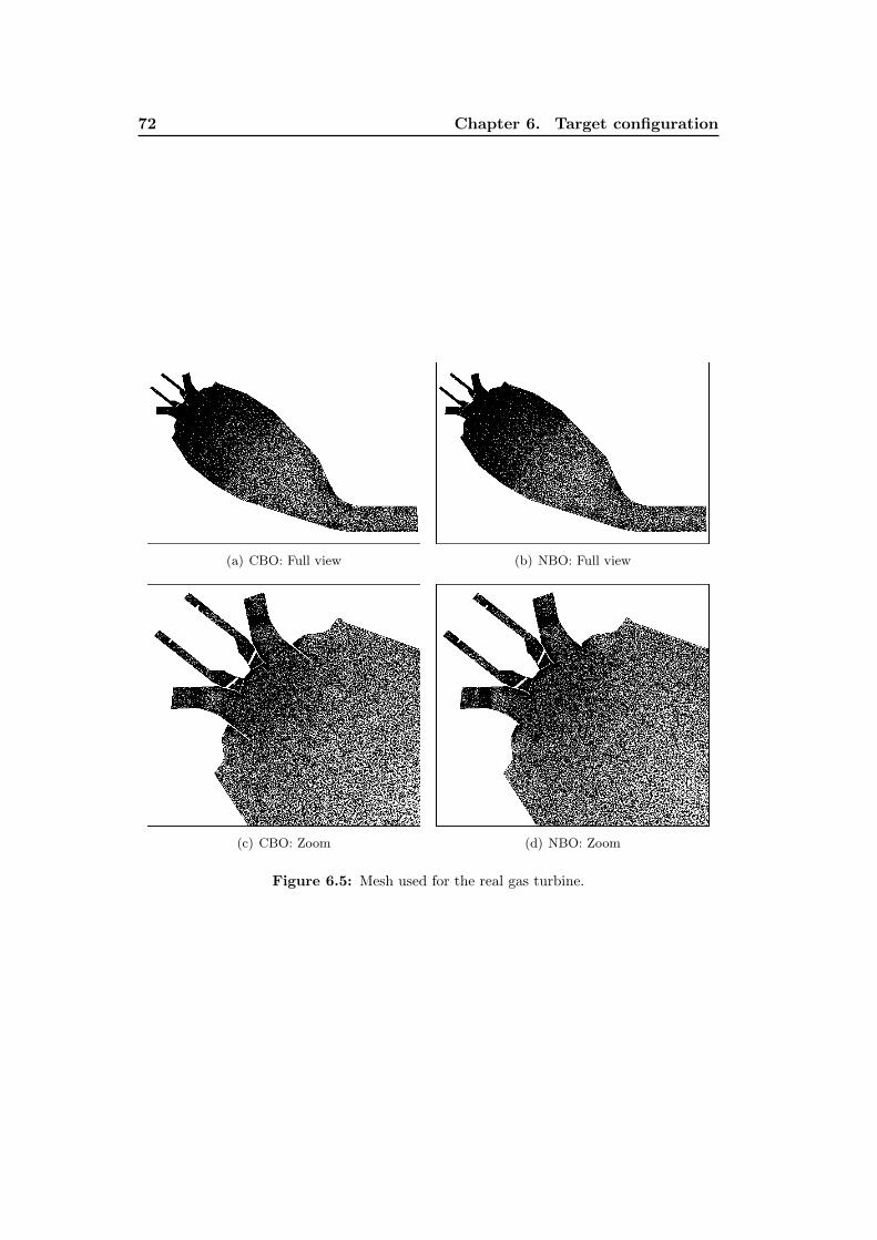
72 Chapter 6. Target configuration
(a) CBO: Full view (b) NBO: Full view
(c) CBO: Zoom (d) NBO: Zoom
Figure 6.5: Mesh used for the real gas turbine.
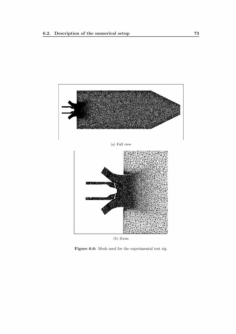
6.2. Description of the numerical setup 73
(a) Full view
(b) Zoom
Figure 6.6: Mesh used for the experimental test rig.
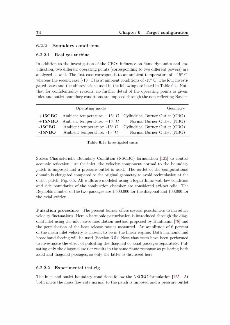
74 Chapter 6. Target configuration
6.2.2 Boundary conditions
6.2.2.1 Real gas turbine
In addition to the investigation of the CBOs influence on flame dynamics and sta-bilisation, two different operating points (corresponding to two different powers) areanalyzed as well. The first case corresponds to an ambient temperature of +15o C,whereas the second case (-15o C) is at ambient conditions of -15o C. The four investi-gated cases and the abbreviations used in the following are listed in Table 6.4. Notethat for confidentiality reasons, no further detail of the operating points is given.Inlet and outlet boundary conditions are imposed through the non-reflecting Navier-
Operating mode Geometry
+15CBO Ambient temperature: +15o C Cylindrical Burner Outlet (CBO)+15NBO Ambient temperature: +15o C Normal Burner Outlet (NBO)-15CBO Ambient temperature: -15o C Cylindrical Burner Outlet (CBO)-15NBO Ambient temperature: -15o C Normal Burner Outlet (NBO)
Table 6.3: Investigated cases
Stokes Characteristic Boundary Condition (NSCBC) formulation [125] to controlacoustic reflection. At the inlet, the velocity component normal to the boundarypatch is imposed and a pressure outlet is used. The outlet of the computationaldomain is elongated compared to the original geometry to avoid recirculation at theoutlet patch, Fig. 6.5. All walls are modeled using a logarithmic wall-law conditionand side boundaries of the combustion chamber are considered axi-periodic. TheReynolds number of the two passages are 1.500.000 for the diagonal and 100.000 forthe axial swirler.
Pulsation procedure The present burner offers several possibilities to introducevelocity fluctuations. Here a harmonic perturbation is introduced through the diag-onal inlet using the inlet wave modulation method proposed by Kaufmann [78] andthe perturbation of the heat release rate is measured. An amplitude of 6 percentof the mean inlet velocity is chosen, to be in the linear regime. Both harmonic andbroadband forcing will be used (Section 3.5). Note that tests have been performedto investigate the effect of pulsating the diagonal or axial passages separately. Pul-sating only the diagonal swirler results in the same flame response as pulsating bothaxial and diagonal passages, so only the latter is discussed here.
6.2.2.2 Experimental test rig
The inlet and outlet boundary conditions follow the NSCBC formulation [125]. Atboth inlets the mass flow rate normal to the patch is imposed and a pressure outlet
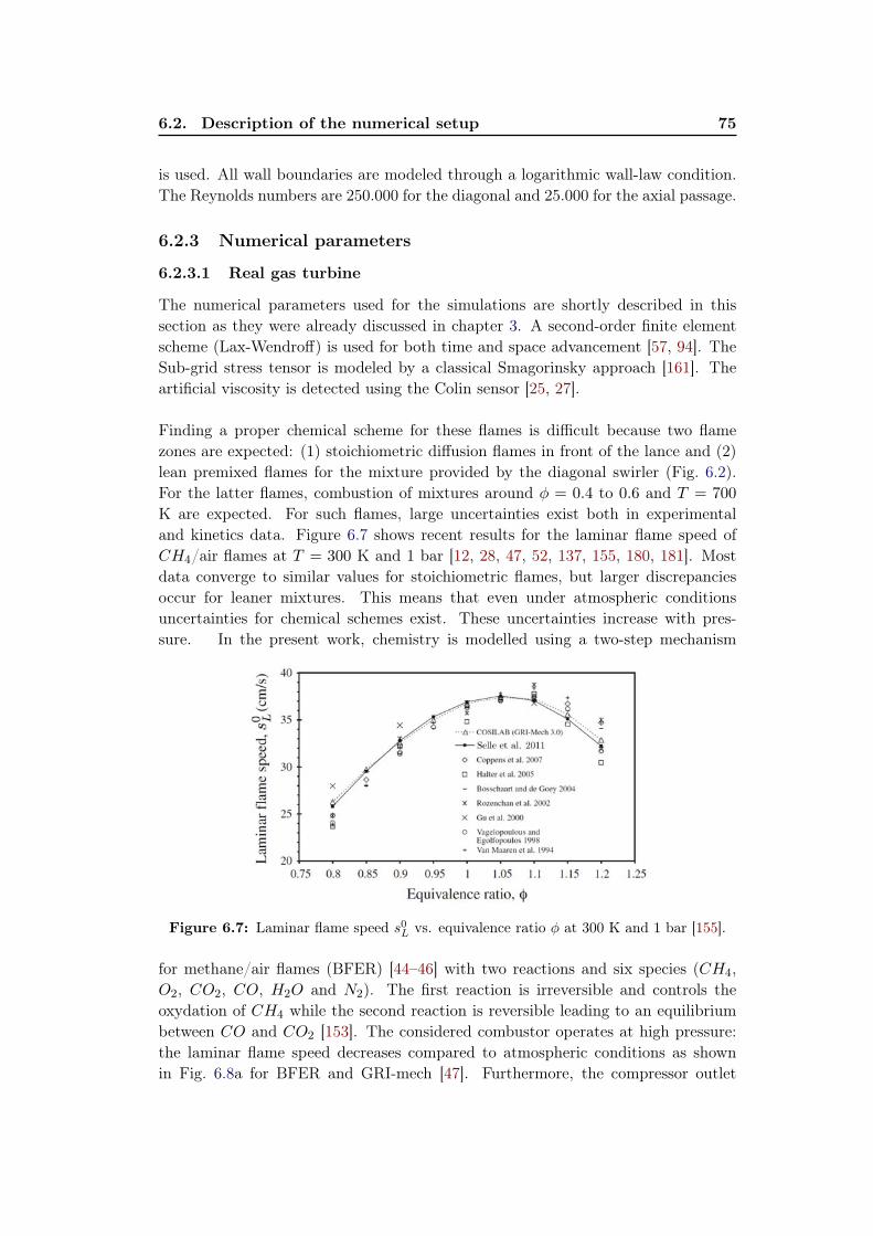
6.2. Description of the numerical setup 75
is used. All wall boundaries are modeled through a logarithmic wall-law condition.The Reynolds numbers are 250.000 for the diagonal and 25.000 for the axial passage.
6.2.3 Numerical parameters
6.2.3.1 Real gas turbine
The numerical parameters used for the simulations are shortly described in thissection as they were already discussed in chapter 3. A second-order finite elementscheme (Lax-Wendroff) is used for both time and space advancement [57, 94]. TheSub-grid stress tensor is modeled by a classical Smagorinsky approach [161]. Theartificial viscosity is detected using the Colin sensor [25, 27].
Finding a proper chemical scheme for these flames is difficult because two flamezones are expected: (1) stoichiometric diffusion flames in front of the lance and (2)lean premixed flames for the mixture provided by the diagonal swirler (Fig. 6.2).For the latter flames, combustion of mixtures around φ = 0.4 to 0.6 and T = 700
K are expected. For such flames, large uncertainties exist both in experimentaland kinetics data. Figure 6.7 shows recent results for the laminar flame speed ofCH4/air flames at T = 300 K and 1 bar [12, 28, 47, 52, 137, 155, 180, 181]. Mostdata converge to similar values for stoichiometric flames, but larger discrepanciesoccur for leaner mixtures. This means that even under atmospheric conditionsuncertainties for chemical schemes exist. These uncertainties increase with pres-sure. In the present work, chemistry is modelled using a two-step mechanism
Figure 6.7: Laminar flame speed s0L vs. equivalence ratio φ at 300 K and 1 bar [155].
for methane/air flames (BFER) [44–46] with two reactions and six species (CH4,O2, CO2, CO, H2O and N2). The first reaction is irreversible and controls theoxydation of CH4 while the second reaction is reversible leading to an equilibriumbetween CO and CO2 [153]. The considered combustor operates at high pressure:the laminar flame speed decreases compared to atmospheric conditions as shownin Fig. 6.8a for BFER and GRI-mech [47]. Furthermore, the compressor outlet
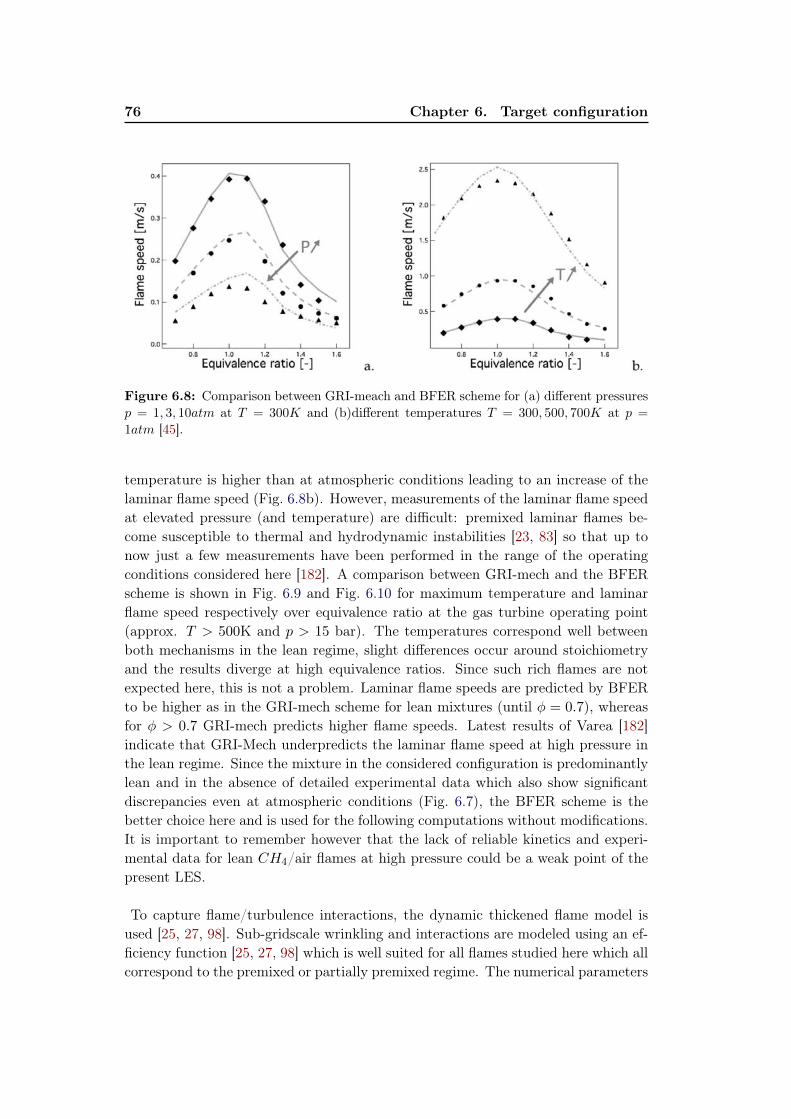
76 Chapter 6. Target configuration
Figure 6.8: Comparison between GRI-meach and BFER scheme for (a) different pressuresp = 1, 3, 10atm at T = 300K and (b)different temperatures T = 300, 500, 700K at p =
1atm [45].
temperature is higher than at atmospheric conditions leading to an increase of thelaminar flame speed (Fig. 6.8b). However, measurements of the laminar flame speedat elevated pressure (and temperature) are difficult: premixed laminar flames be-come susceptible to thermal and hydrodynamic instabilities [23, 83] so that up tonow just a few measurements have been performed in the range of the operatingconditions considered here [182]. A comparison between GRI-mech and the BFERscheme is shown in Fig. 6.9 and Fig. 6.10 for maximum temperature and laminarflame speed respectively over equivalence ratio at the gas turbine operating point(approx. T > 500K and p > 15 bar). The temperatures correspond well betweenboth mechanisms in the lean regime, slight differences occur around stoichiometryand the results diverge at high equivalence ratios. Since such rich flames are notexpected here, this is not a problem. Laminar flame speeds are predicted by BFERto be higher as in the GRI-mech scheme for lean mixtures (until φ = 0.7), whereasfor φ > 0.7 GRI-mech predicts higher flame speeds. Latest results of Varea [182]indicate that GRI-Mech underpredicts the laminar flame speed at high pressure inthe lean regime. Since the mixture in the considered configuration is predominantlylean and in the absence of detailed experimental data which also show significantdiscrepancies even at atmospheric conditions (Fig. 6.7), the BFER scheme is thebetter choice here and is used for the following computations without modifications.It is important to remember however that the lack of reliable kinetics and experi-mental data for lean CH4/air flames at high pressure could be a weak point of thepresent LES.
To capture flame/turbulence interactions, the dynamic thickened flame model isused [25, 27, 98]. Sub-gridscale wrinkling and interactions are modeled using an ef-ficiency function [25, 27, 98] which is well suited for all flames studied here which allcorrespond to the premixed or partially premixed regime. The numerical parameters

6.2. Description of the numerical setup 77
Figure 6.9: Temperature over equivalence ratio for GRI-Mech and BFER for CH4/airflames at T = 700 K and p = 17 bar.
Figure 6.10: Laminar flame speed over equivalence ratio for GRI-Mech and BFER forCH4/air flames at T = 700 K and p = 17 bar.
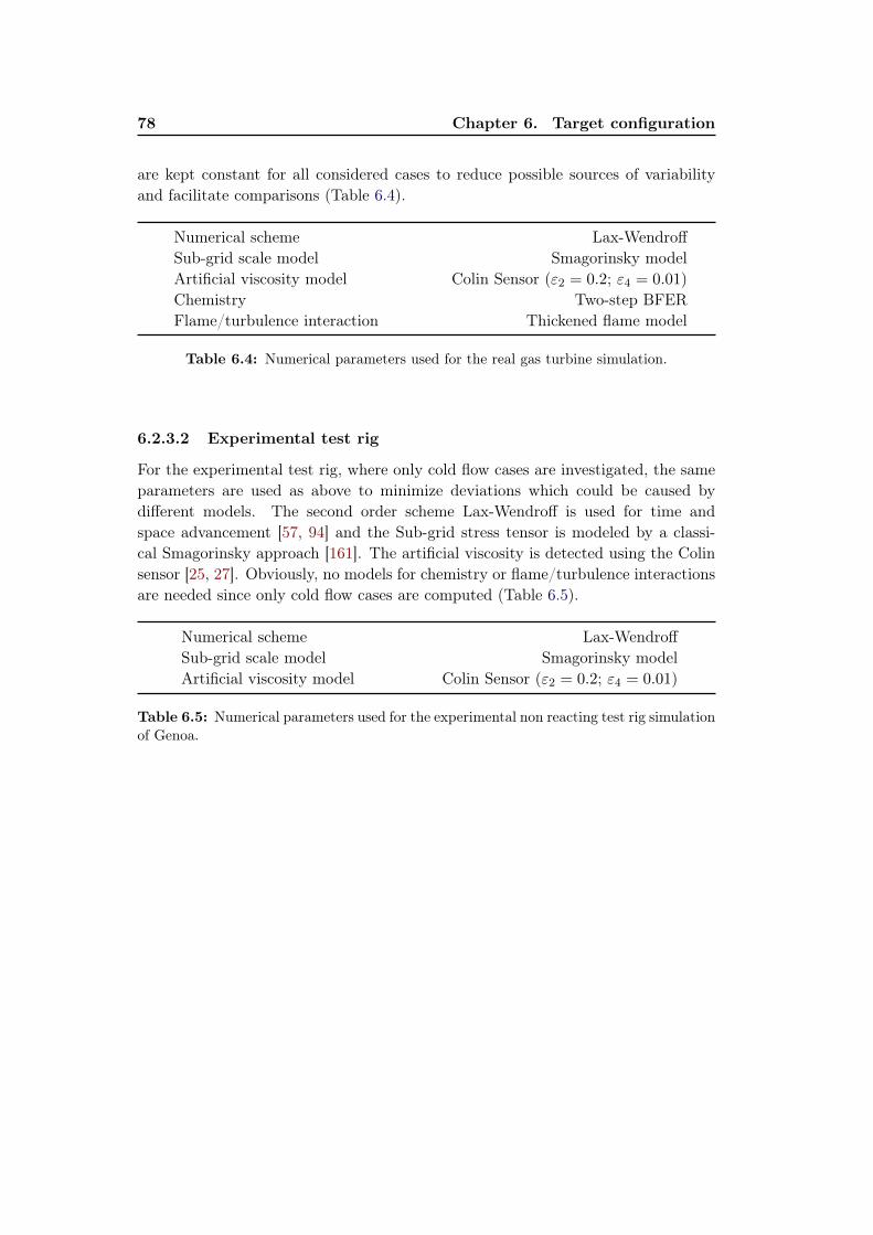
78 Chapter 6. Target configuration
are kept constant for all considered cases to reduce possible sources of variabilityand facilitate comparisons (Table 6.4).
Numerical scheme Lax-WendroffSub-grid scale model Smagorinsky modelArtificial viscosity model Colin Sensor (ε2 = 0.2; ε4 = 0.01)Chemistry Two-step BFERFlame/turbulence interaction Thickened flame model
Table 6.4: Numerical parameters used for the real gas turbine simulation.
6.2.3.2 Experimental test rig
For the experimental test rig, where only cold flow cases are investigated, the sameparameters are used as above to minimize deviations which could be caused bydifferent models. The second order scheme Lax-Wendroff is used for time andspace advancement [57, 94] and the Sub-grid stress tensor is modeled by a classi-cal Smagorinsky approach [161]. The artificial viscosity is detected using the Colinsensor [25, 27]. Obviously, no models for chemistry or flame/turbulence interactionsare needed since only cold flow cases are computed (Table 6.5).
Numerical scheme Lax-WendroffSub-grid scale model Smagorinsky modelArtificial viscosity model Colin Sensor (ε2 = 0.2; ε4 = 0.01)
Table 6.5: Numerical parameters used for the experimental non reacting test rig simulationof Genoa.
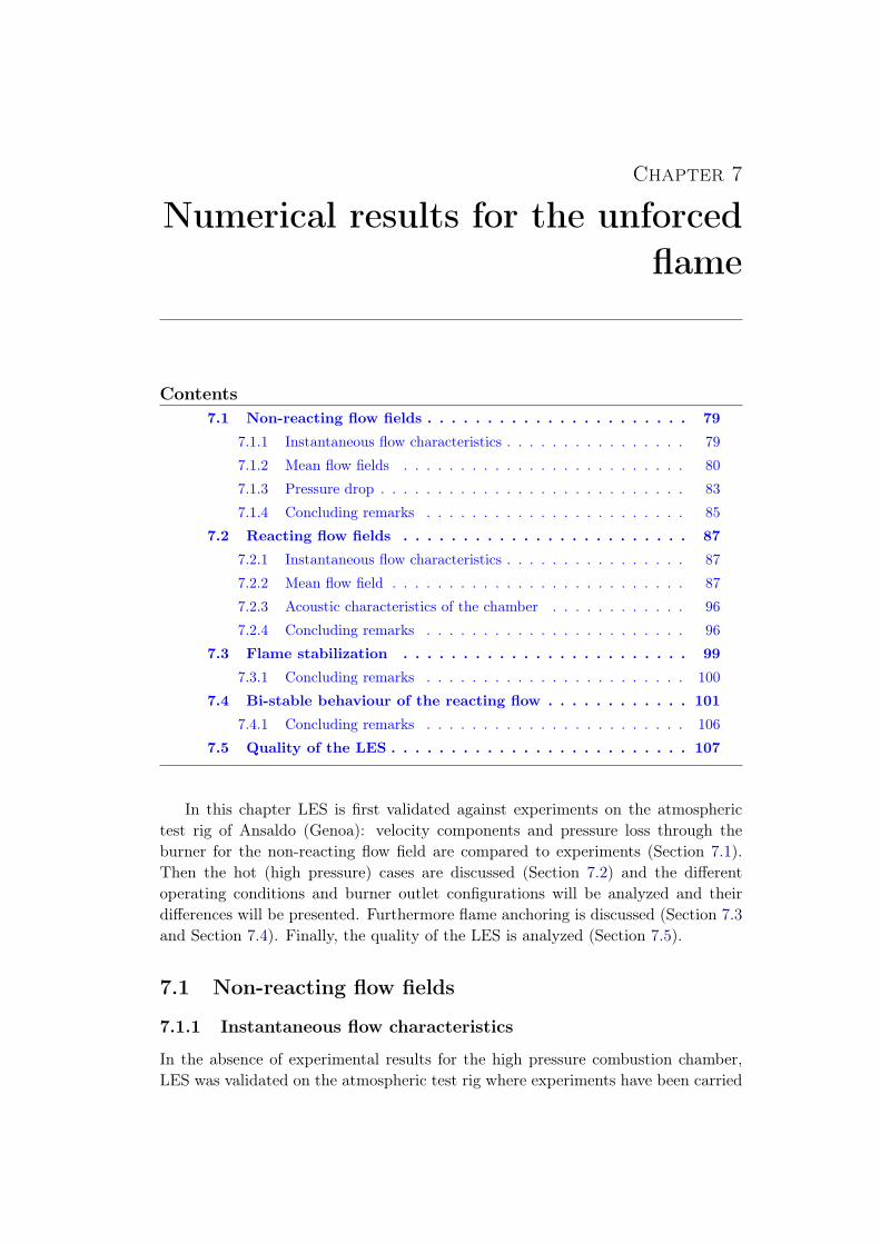
Chapter 7
Numerical results for the unforcedflame
Contents7.1 Non-reacting flow fields . . . . . . . . . . . . . . . . . . . . . . 79
7.1.1 Instantaneous flow characteristics . . . . . . . . . . . . . . . . 79
7.1.2 Mean flow fields . . . . . . . . . . . . . . . . . . . . . . . . . 80
7.1.3 Pressure drop . . . . . . . . . . . . . . . . . . . . . . . . . . . 83
7.1.4 Concluding remarks . . . . . . . . . . . . . . . . . . . . . . . 85
7.2 Reacting flow fields . . . . . . . . . . . . . . . . . . . . . . . . 87
7.2.1 Instantaneous flow characteristics . . . . . . . . . . . . . . . . 87
7.2.2 Mean flow field . . . . . . . . . . . . . . . . . . . . . . . . . . 87
7.2.3 Acoustic characteristics of the chamber . . . . . . . . . . . . 96
7.2.4 Concluding remarks . . . . . . . . . . . . . . . . . . . . . . . 96
7.3 Flame stabilization . . . . . . . . . . . . . . . . . . . . . . . . 99
7.3.1 Concluding remarks . . . . . . . . . . . . . . . . . . . . . . . 100
7.4 Bi-stable behaviour of the reacting flow . . . . . . . . . . . . 101
7.4.1 Concluding remarks . . . . . . . . . . . . . . . . . . . . . . . 106
7.5 Quality of the LES . . . . . . . . . . . . . . . . . . . . . . . . . 107
In this chapter LES is first validated against experiments on the atmospherictest rig of Ansaldo (Genoa): velocity components and pressure loss through theburner for the non-reacting flow field are compared to experiments (Section 7.1).Then the hot (high pressure) cases are discussed (Section 7.2) and the differentoperating conditions and burner outlet configurations will be analyzed and theirdifferences will be presented. Furthermore flame anchoring is discussed (Section 7.3and Section 7.4). Finally, the quality of the LES is analyzed (Section 7.5).
7.1 Non-reacting flow fields
7.1.1 Instantaneous flow characteristics
In the absence of experimental results for the high pressure combustion chamber,LES was validated on the atmospheric test rig where experiments have been carried

80 Chapter 7. Numerical results for the unforced flame
out. The Reynolds number in the combustion chamber is of order of 1.000.000. Forsuch high Reynolds number flows, LES is difficult and validation mandatory. Notealso that performing experimental measurements is also much more difficult than inlab-scale set-ups. PIV measurements at the cut plane (Fig. 6.4) just downstream ofthe burner outlet allow the comparison of different velocity components. Further-more the pressure drop through the burner will be evaluated and compared againstpressure measurements obtained in Genoa.
Swirling flows feature several types of vortex breakdown [106] and can lead to theformation of so-called precessing vortex cores (PVC). The PVC is a well knownlarge scale hydrodynamic structure occurring at high Reynolds and swirl numberflows [51, 53, 63, 135, 136, 153, 157]. It is characterized by a regular rotation ofa spiral structure around the geometrical axis of the combustion chamber and isshown for the considered configuration in Fig. 7.1 for one cycle. The frequency pre-dicted by LES matches the experiments and is 120 Hz corresponding to a StrouhalSt = fD/ubulk = 1.3 based on the burner diameter D and the bulk velocity ubulk.The present vortex breakdown results from a highly swirled flow and leads in com-bination with the sudden geometrical expansion at the combustion chamber inletto a recirculation of the flow. An outer and a inner recirculation zone is formedand interacts with the hydrodynamic instability of the PVC. The resulting averagedmean flow field is shown in the following.
7.1.2 Mean flow fields
The PVC influences the mean axial velocity field shown in Fig. 7.2 on the middlecut plane. For this swirler with multiple passages, the flow topology is more com-plicated than in usual swirling flows. Here, two recirculation zones are found on thechamber axis. As indicated by the zero velocity iso-lines, negative velocity occursfirst close to the lance followed by a region of positive velocity and finally by themain inner recirculation zone. The positive velocity region results form the PVCwhose low pressure vortex core sucks the flow in the direction of the geometricalaxis and dependent on their position along the axis, either the upper flow of thediagonal swirler is deviated or the lower part so that the inner recirculation zonefinally underlies strong variations. In the averaged field this is seen as a positiveaxial velocity region. Comparison to the PIV experiments in Fig. 7.4 for the ax-ial velocity on the measurement plane (Fig. 7.3) just in front of the burner outletshows differences: in the center LES predicts low positive values but PIV show lownegative axial velocities. From the center to the CBO in radial direction, the axialvelocity increases significantly with a similar amplitude between PIV and LES. Notethat experiments were not performed in the region radially outside the CBO andare marked as zero velocities. The velocities in y- and z direction are comparedin Fig. 7.5 and Fig. 7.6 respectively. Experiments and LES agree: the y-velocity ismaximal in magnitude on the upper and lower side with opposite sign. The samebehaviour is seen for the z-velocity where the maximal magnitude appears on the
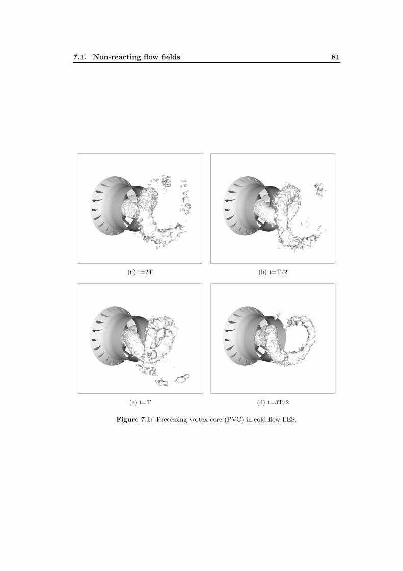
7.1. Non-reacting flow fields 81
(a) t=2T (b) t=T/2
(c) t=T (d) t=3T/2
Figure 7.1: Precessing vortex core (PVC) in cold flow LES.

82 Chapter 7. Numerical results for the unforced flame
Figure 7.2: Mean axial velocity field on middle cut plane. The white line corresponds tozero axial velocity.
Figure 7.3: Reference plane location.

7.1. Non-reacting flow fields 83
Figure 7.4: Axial-velocity: comparison PIV and LES.
right and left side. The positions of peaks and zero velocities are in good agreementfor both velocity components. Furthermore, similar tangential velocity fields are
Figure 7.5: y-velocity: comparison PIV and LES.
found (Fig. 7.7). The lowest velocity is found in the center and increases in theradial direction. LES slightly under predicts the magnitude in the outer region andpredicts an almost uniform distribution at fixed radius whereas PIV shows a highervelocity magnitude in the top and bottom regions.
7.1.3 Pressure drop
Another possibility to evaluate the quality of LES is to compare the pressure dropthrough the burner against measurements. A convenient way to quantify pressure

84 Chapter 7. Numerical results for the unforced flame
Figure 7.6: z-velocity: comparison PIV and LES.
Figure 7.7: Tangential velocity: comparison PIV and LES.
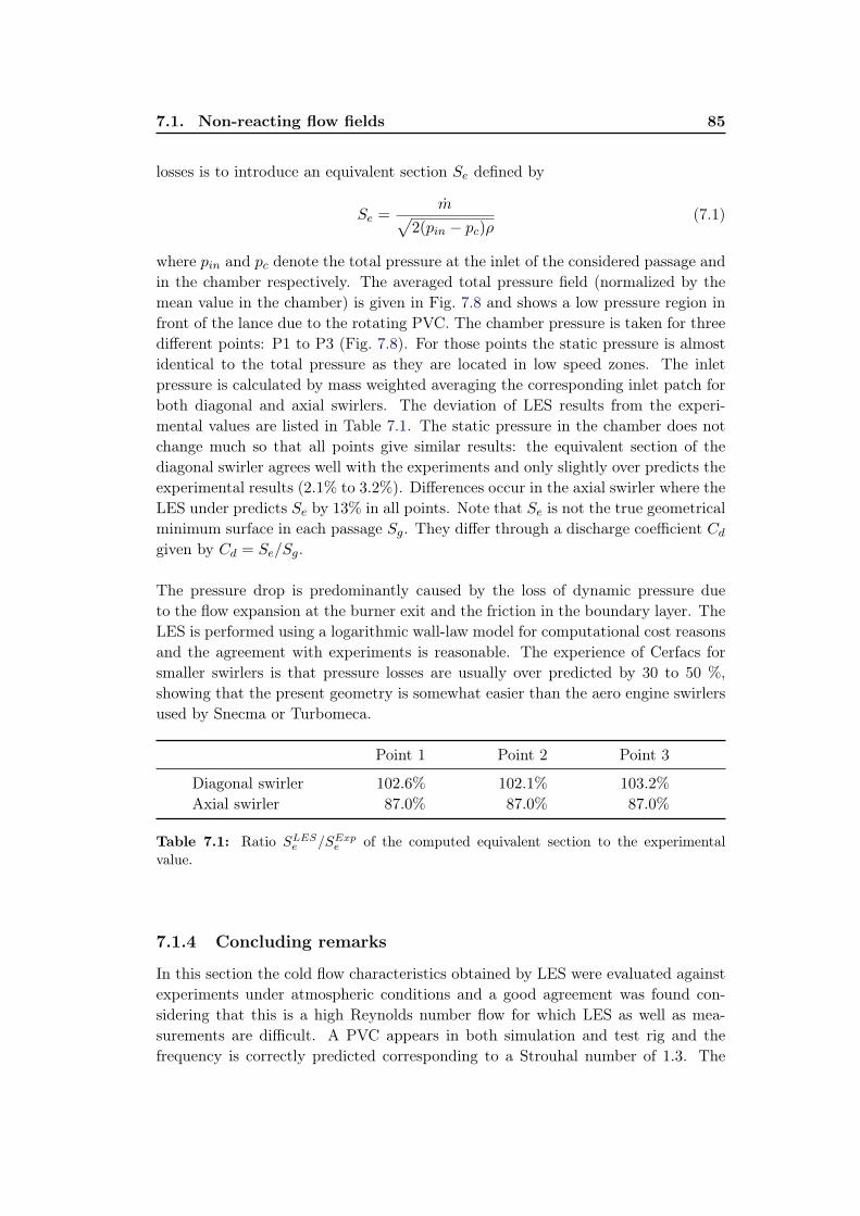
7.1. Non-reacting flow fields 85
losses is to introduce an equivalent section Se defined by
Se =m√
2(pin − pc)ρ(7.1)
where pin and pc denote the total pressure at the inlet of the considered passage andin the chamber respectively. The averaged total pressure field (normalized by themean value in the chamber) is given in Fig. 7.8 and shows a low pressure region infront of the lance due to the rotating PVC. The chamber pressure is taken for threedifferent points: P1 to P3 (Fig. 7.8). For those points the static pressure is almostidentical to the total pressure as they are located in low speed zones. The inletpressure is calculated by mass weighted averaging the corresponding inlet patch forboth diagonal and axial swirlers. The deviation of LES results from the experi-mental values are listed in Table 7.1. The static pressure in the chamber does notchange much so that all points give similar results: the equivalent section of thediagonal swirler agrees well with the experiments and only slightly over predicts theexperimental results (2.1% to 3.2%). Differences occur in the axial swirler where theLES under predicts Se by 13% in all points. Note that Se is not the true geometricalminimum surface in each passage Sg. They differ through a discharge coefficient Cdgiven by Cd = Se/Sg.
The pressure drop is predominantly caused by the loss of dynamic pressure dueto the flow expansion at the burner exit and the friction in the boundary layer. TheLES is performed using a logarithmic wall-law model for computational cost reasonsand the agreement with experiments is reasonable. The experience of Cerfacs forsmaller swirlers is that pressure losses are usually over predicted by 30 to 50 %,showing that the present geometry is somewhat easier than the aero engine swirlersused by Snecma or Turbomeca.
Point 1 Point 2 Point 3
Diagonal swirler 102.6% 102.1% 103.2%Axial swirler 87.0% 87.0% 87.0%
Table 7.1: Ratio SLESe /SExpe of the computed equivalent section to the experimentalvalue.
7.1.4 Concluding remarks
In this section the cold flow characteristics obtained by LES were evaluated againstexperiments under atmospheric conditions and a good agreement was found con-sidering that this is a high Reynolds number flow for which LES as well as mea-surements are difficult. A PVC appears in both simulation and test rig and thefrequency is correctly predicted corresponding to a Strouhal number of 1.3. The
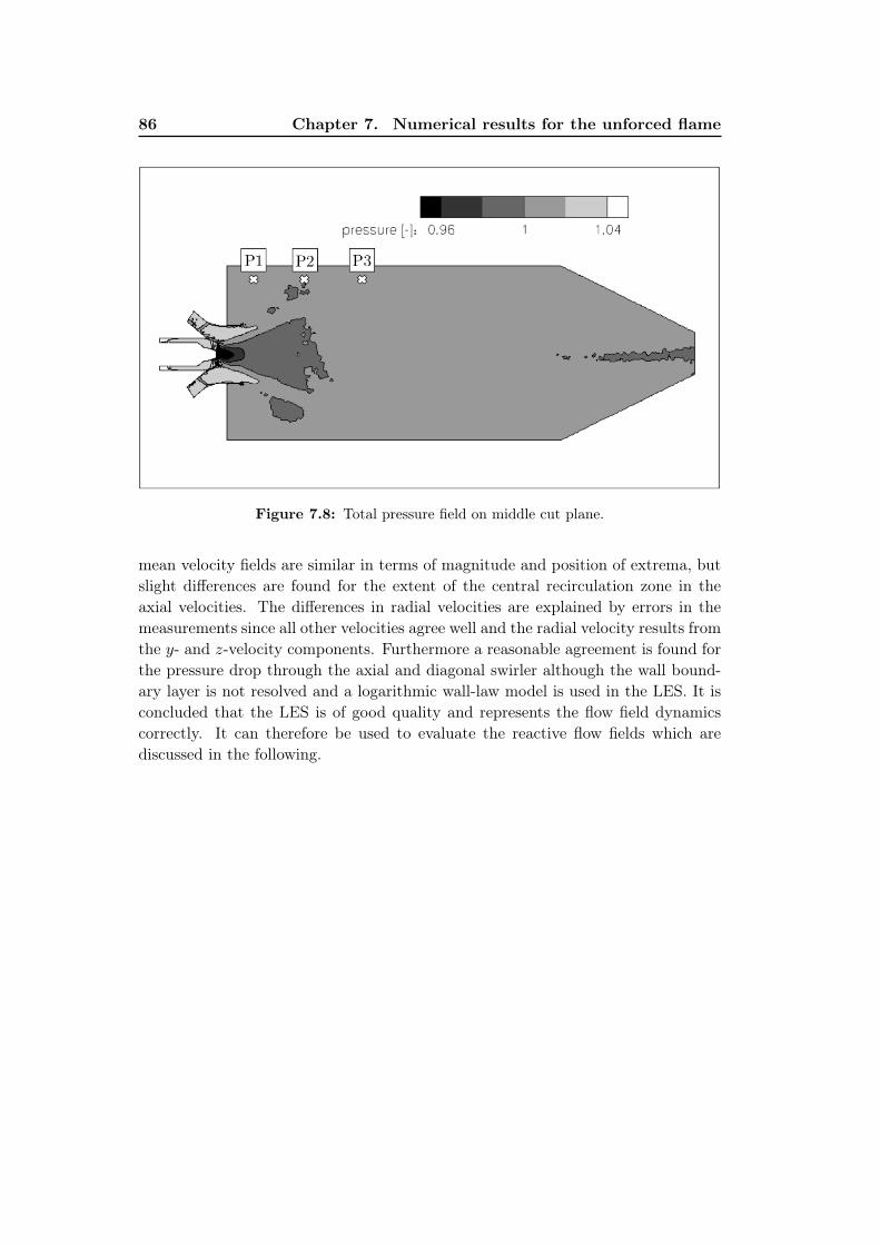
86 Chapter 7. Numerical results for the unforced flame
Figure 7.8: Total pressure field on middle cut plane.
mean velocity fields are similar in terms of magnitude and position of extrema, butslight differences are found for the extent of the central recirculation zone in theaxial velocities. The differences in radial velocities are explained by errors in themeasurements since all other velocities agree well and the radial velocity results fromthe y- and z-velocity components. Furthermore a reasonable agreement is found forthe pressure drop through the axial and diagonal swirler although the wall bound-ary layer is not resolved and a logarithmic wall-law model is used in the LES. It isconcluded that the LES is of good quality and represents the flow field dynamicscorrectly. It can therefore be used to evaluate the reactive flow fields which arediscussed in the following.
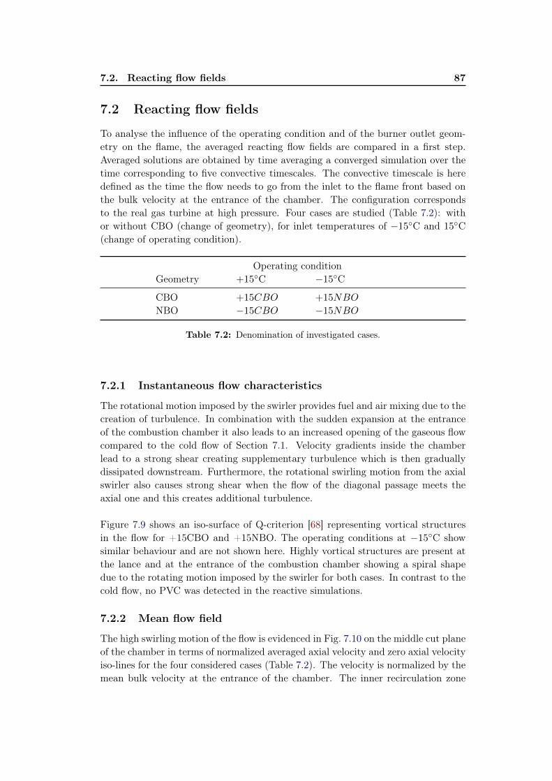
7.2. Reacting flow fields 87
7.2 Reacting flow fields
To analyse the influence of the operating condition and of the burner outlet geom-etry on the flame, the averaged reacting flow fields are compared in a first step.Averaged solutions are obtained by time averaging a converged simulation over thetime corresponding to five convective timescales. The convective timescale is heredefined as the time the flow needs to go from the inlet to the flame front based onthe bulk velocity at the entrance of the chamber. The configuration correspondsto the real gas turbine at high pressure. Four cases are studied (Table 7.2): withor without CBO (change of geometry), for inlet temperatures of −15◦C and 15◦C(change of operating condition).
Operating conditionGeometry +15◦C −15◦C
CBO +15CBO +15NBO
NBO −15CBO −15NBO
Table 7.2: Denomination of investigated cases.
7.2.1 Instantaneous flow characteristics
The rotational motion imposed by the swirler provides fuel and air mixing due to thecreation of turbulence. In combination with the sudden expansion at the entranceof the combustion chamber it also leads to an increased opening of the gaseous flowcompared to the cold flow of Section 7.1. Velocity gradients inside the chamberlead to a strong shear creating supplementary turbulence which is then graduallydissipated downstream. Furthermore, the rotational swirling motion from the axialswirler also causes strong shear when the flow of the diagonal passage meets theaxial one and this creates additional turbulence.
Figure 7.9 shows an iso-surface of Q-criterion [68] representing vortical structuresin the flow for +15CBO and +15NBO. The operating conditions at −15◦C showsimilar behaviour and are not shown here. Highly vortical structures are present atthe lance and at the entrance of the combustion chamber showing a spiral shapedue to the rotating motion imposed by the swirler for both cases. In contrast to thecold flow, no PVC was detected in the reactive simulations.
7.2.2 Mean flow field
The high swirling motion of the flow is evidenced in Fig. 7.10 on the middle cut planeof the chamber in terms of normalized averaged axial velocity and zero axial velocityiso-lines for the four considered cases (Table 7.2). The velocity is normalized by themean bulk velocity at the entrance of the chamber. The inner recirculation zone
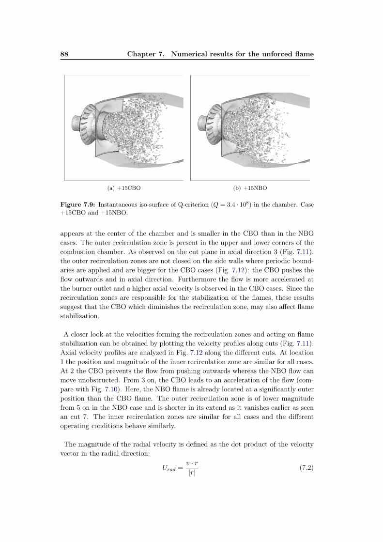
88 Chapter 7. Numerical results for the unforced flame
(a) +15CBO (b) +15NBO
Figure 7.9: Instantaneous iso-surface of Q-criterion (Q = 3.4 · 108) in the chamber. Case+15CBO and +15NBO.
appears at the center of the chamber and is smaller in the CBO than in the NBOcases. The outer recirculation zone is present in the upper and lower corners of thecombustion chamber. As observed on the cut plane in axial direction 3 (Fig. 7.11),the outer recirculation zones are not closed on the side walls where periodic bound-aries are applied and are bigger for the CBO cases (Fig. 7.12): the CBO pushes theflow outwards and in axial direction. Furthermore the flow is more accelerated atthe burner outlet and a higher axial velocity is observed in the CBO cases. Since therecirculation zones are responsible for the stabilization of the flames, these resultssuggest that the CBO which diminishes the recirculation zone, may also affect flamestabilization.
A closer look at the velocities forming the recirculation zones and acting on flamestabilization can be obtained by plotting the velocity profiles along cuts (Fig. 7.11).Axial velocity profiles are analyzed in Fig. 7.12 along the different cuts. At location1 the position and magnitude of the inner recirculation zone are similar for all cases.At 2 the CBO prevents the flow from pushing outwards whereas the NBO flow canmove unobstructed. From 3 on, the CBO leads to an acceleration of the flow (com-pare with Fig. 7.10). Here, the NBO flame is already located at a significantly outerposition than the CBO flame. The outer recirculation zone is of lower magnitudefrom 5 on in the NBO case and is shorter in its extend as it vanishes earlier as seenan cut 7. The inner recirculation zones are similar for all cases and the differentoperating conditions behave similarly.
The magnitude of the radial velocity is defined as the dot product of the velocityvector in the radial direction:
Urad =v · r|r|
(7.2)
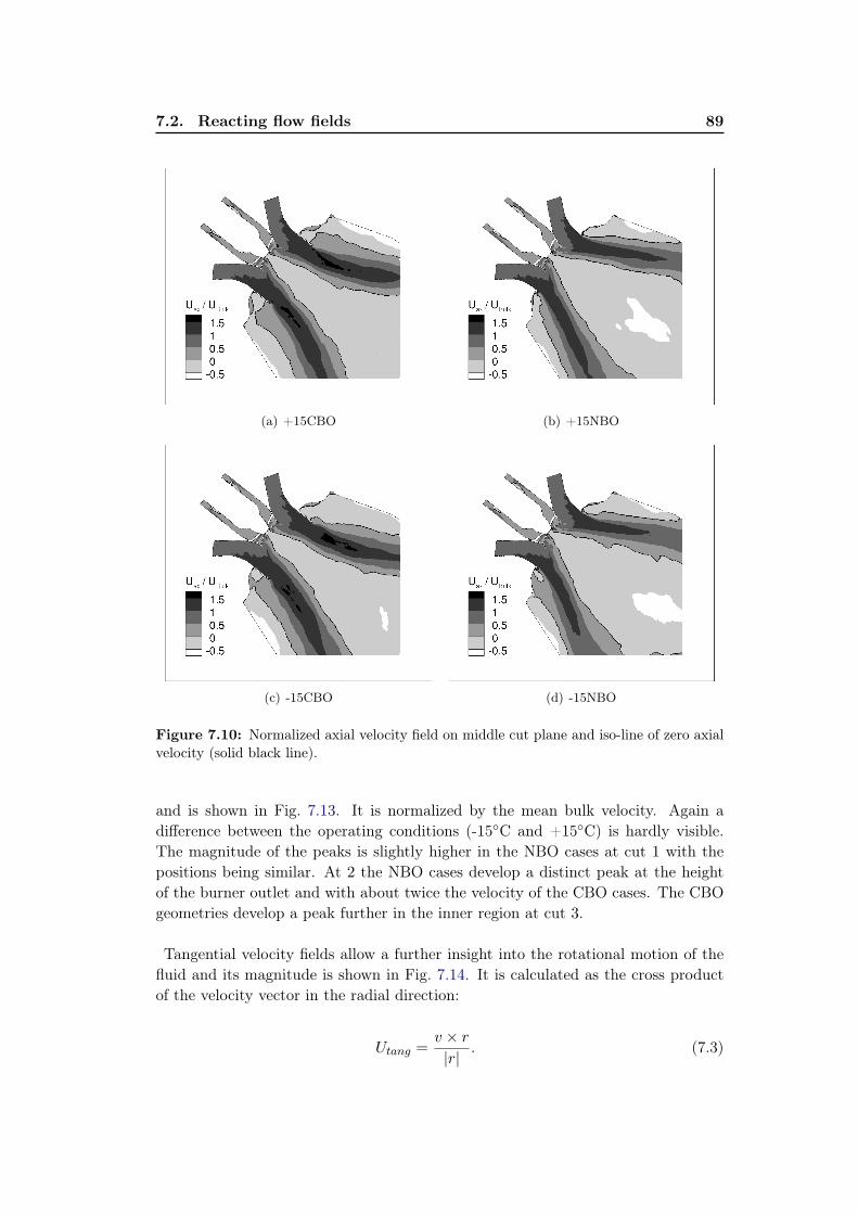
7.2. Reacting flow fields 89
(a) +15CBO (b) +15NBO
(c) -15CBO (d) -15NBO
Figure 7.10: Normalized axial velocity field on middle cut plane and iso-line of zero axialvelocity (solid black line).
and is shown in Fig. 7.13. It is normalized by the mean bulk velocity. Again adifference between the operating conditions (-15◦C and +15◦C) is hardly visible.The magnitude of the peaks is slightly higher in the NBO cases at cut 1 with thepositions being similar. At 2 the NBO cases develop a distinct peak at the heightof the burner outlet and with about twice the velocity of the CBO cases. The CBOgeometries develop a peak further in the inner region at cut 3.
Tangential velocity fields allow a further insight into the rotational motion of thefluid and its magnitude is shown in Fig. 7.14. It is calculated as the cross productof the velocity vector in the radial direction:
Utang =v × r|r|
. (7.3)

90 Chapter 7. Numerical results for the unforced flame
Figure 7.11: Planes for profile extraction
−2 0 2−1
−0.8
−0.6
−0.4
−0.2
0
0.2
0.4
0.6
0.8
1
y/y
ma
x [
−]
1
−2 0 2
2
−2 0 2
3
−2 0 2
Uax
/Ubulk
[−]
4
−2 0 2
5
−2 0 2
6
+15CBO
+15NBO
−15CBO
−15NBO
−2 0 2
7
Figure 7.12: Axial velocity profiles for +15CBO, +15NBO, -15CBO, -15NBO

7.2. Reacting flow fields 91
All flames behave similarly in terms of tangential velocity close to the lance wherethe peak shows a only slightly decreasing magnitude to outer direction. As the flameopens in the NBO cases, the peaks is further away from the axis but with similarmagnitude compared to the CBO cases. No distinctive differences can be foundbetween the operating conditions +15 and -15. The interaction of those differentvelocity components control the flame and are directly responsible for its stabiliza-tion and dynamics.
Figure 7.15 shows the three-dimensional flame surface obtained with a tempera-ture iso-surface (T/Tmean = 1.3) and coloured by the axial velocity for the fourinvestigated cases. The negative axial velocities from the inner recirculation zones(Fig. 7.10) anchor all flames at the lance and in combination with the outer recir-culation zones the flames attach at the burner outlet. Nevertheless, the differentshapes of the recirculation zones and the associated velocity profiles affect the flamesdirectly. The CBO elongates and narrows the flame for both operating conditionswhile the NBO flame is distinctively shorter and more open. Although the outerrecirculation zones are only present in the upper and lower walls of the combustionchamber, the flames are closed and completely attached to the burner outlet. In allcases the lowest velocity appears at the burner outlet with increasing velocities upto the flame tip. The temperature field on the middle cut plane (Fig. 7.16) revealsthat the highest temperature occurs at the lance where pure methane stabilizes theflame through the pilot injection. The averaged flame shapes and axial velocityfields are similar for the two operating conditions.
The temperature profiles reveal more details about the flame shapes (Fig. 7.17).Similar normalized temperature profiles between the operating conditions are found.The burner outlet geometry has a great impact: close to the lance (profile 1) all fourprofiles are similar and show the highest temperature being twice the mean valuewhich is due to the pilot injection where a high local equivalence ratio is present.At cut 2 the NBO flame is significantly more open showing the same temperaturemagnitude as the CBO case. Downstream of location 3, minima have a highertemperature for the NBO geometry because the flame is shorter. All cases reach asimilar temperature in the burnt gases and are axi-symmetric.
To obtain further insight on the mechanisms at play insuring flame stabilization,the fluctuations of temperature in Fig. 7.18 are investigated. Both operating condi-tions (-15◦C and +15◦C) show similar fluctuations. In both burner configurationstwo distinct peaks appear and merge downstream. Since the NBO flame is shorter,the fluctuations vanish earlier and are higher close to the lance at cut 2.

92 Chapter 7. Numerical results for the unforced flame
−1 0 1−1
−0.8
−0.6
−0.4
−0.2
0
0.2
0.4
0.6
0.8
1
y/y
ma
x [
−]
1
−1 0 1
2
−1 0 1
3
−1 0 1
Urad
/Ubulk
[−]
4
−1 0 1
5
−1 0 1
6
−1 0 1
7
+15CBO
+15NBO
−15CBO
−15NBO
Figure 7.13: Radial velocity profiles for +15CBO, +15NBO, -15CBO, -15NBO
−0.5 0.5 1.5−1
−0.8
−0.6
−0.4
−0.2
0
0.2
0.4
0.6
0.8
1
y/y
ma
x [
−]
1
−0.5 0.5 1.5
2
−0.5 0.5 1.5
3
−0.5 0.5 1.5
Utang
/Ubulk
[−]
4
−0.5 0.5 1.5
5
−0.5 0.5 1.5
6
−0.5 0.5 1.5
7
+15CBO
+15NBO
−15CBO
−15NBO
Figure 7.14: Tangential velocity profiles for +15CBO, +15NBO, -15CBO, -15NBO
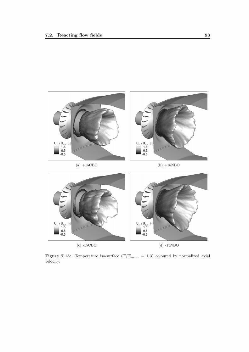
7.2. Reacting flow fields 93
(a) +15CBO (b) +15NBO
(c) -15CBO (d) -15NBO
Figure 7.15: Temperature iso-surface (T/Tmean = 1.3) coloured by normalized axialvelocity.

94 Chapter 7. Numerical results for the unforced flame
(a) +15CBO (b) +15NBO
(c) -15CBO (d) -15NBO
Figure 7.16: Normalized temperature field on middle cut plane.
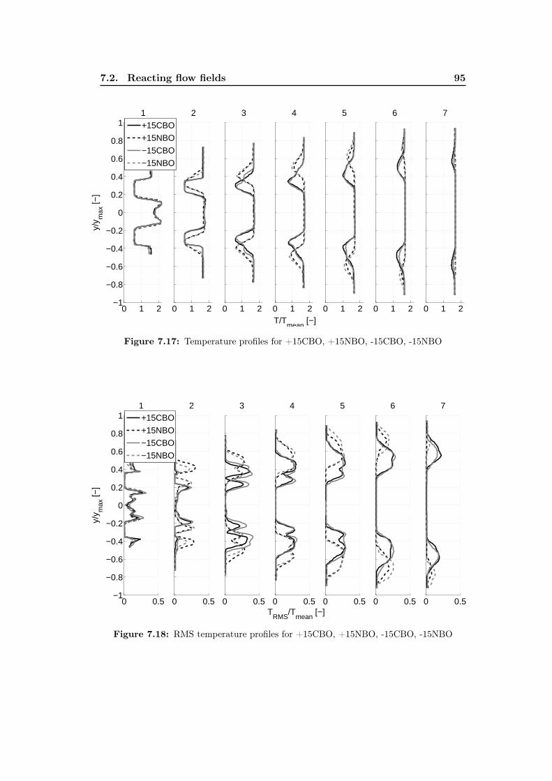
7.2. Reacting flow fields 95
0 1 2−1
−0.8
−0.6
−0.4
−0.2
0
0.2
0.4
0.6
0.8
1
y/y
ma
x [
−]
1
0 1 2
2
0 1 2
3
0 1 2
T/Tmean
[−]
4
0 1 2
5
0 1 2
6
0 1 2
7
+15CBO
+15NBO
−15CBO
−15NBO
Figure 7.17: Temperature profiles for +15CBO, +15NBO, -15CBO, -15NBO
0 0.5−1
−0.8
−0.6
−0.4
−0.2
0
0.2
0.4
0.6
0.8
1
y/y
ma
x [
−]
1
0 0.5
2
0 0.5
3
0 0.5
TRMS
/Tmean
[−]
4
0 0.5
5
0 0.5
6
0 0.5
7
+15CBO
+15NBO
−15CBO
−15NBO
Figure 7.18: RMS temperature profiles for +15CBO, +15NBO, -15CBO, -15NBO
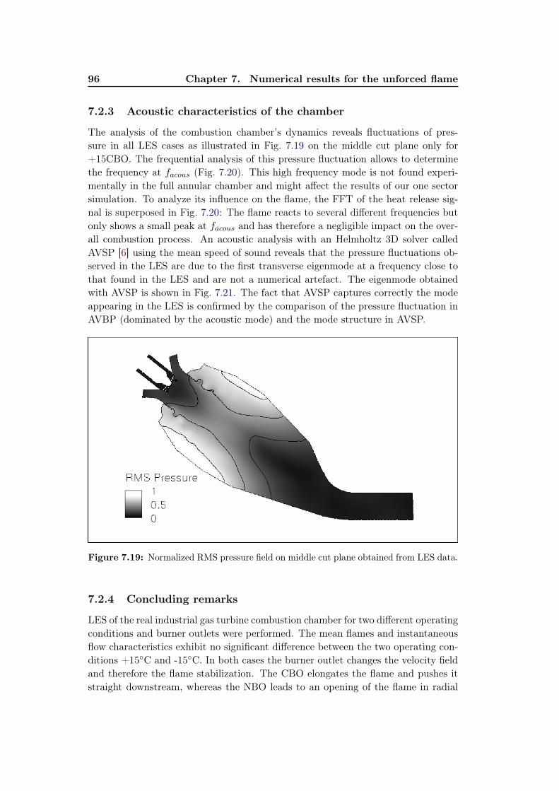
96 Chapter 7. Numerical results for the unforced flame
7.2.3 Acoustic characteristics of the chamber
The analysis of the combustion chamber’s dynamics reveals fluctuations of pres-sure in all LES cases as illustrated in Fig. 7.19 on the middle cut plane only for+15CBO. The frequential analysis of this pressure fluctuation allows to determinethe frequency at facous (Fig. 7.20). This high frequency mode is not found experi-mentally in the full annular chamber and might affect the results of our one sectorsimulation. To analyze its influence on the flame, the FFT of the heat release sig-nal is superposed in Fig. 7.20: The flame reacts to several different frequencies butonly shows a small peak at facous and has therefore a negligible impact on the over-all combustion process. An acoustic analysis with an Helmholtz 3D solver calledAVSP [6] using the mean speed of sound reveals that the pressure fluctuations ob-served in the LES are due to the first transverse eigenmode at a frequency close tothat found in the LES and are not a numerical artefact. The eigenmode obtainedwith AVSP is shown in Fig. 7.21. The fact that AVSP captures correctly the modeappearing in the LES is confirmed by the comparison of the pressure fluctuation inAVBP (dominated by the acoustic mode) and the mode structure in AVSP.
Figure 7.19: Normalized RMS pressure field on middle cut plane obtained from LES data.
7.2.4 Concluding remarks
LES of the real industrial gas turbine combustion chamber for two different operatingconditions and burner outlets were performed. The mean flames and instantaneousflow characteristics exhibit no significant difference between the two operating con-ditions +15◦C and -15◦C. In both cases the burner outlet changes the velocity fieldand therefore the flame stabilization. The CBO elongates the flame and pushes itstraight downstream, whereas the NBO leads to an opening of the flame in radial
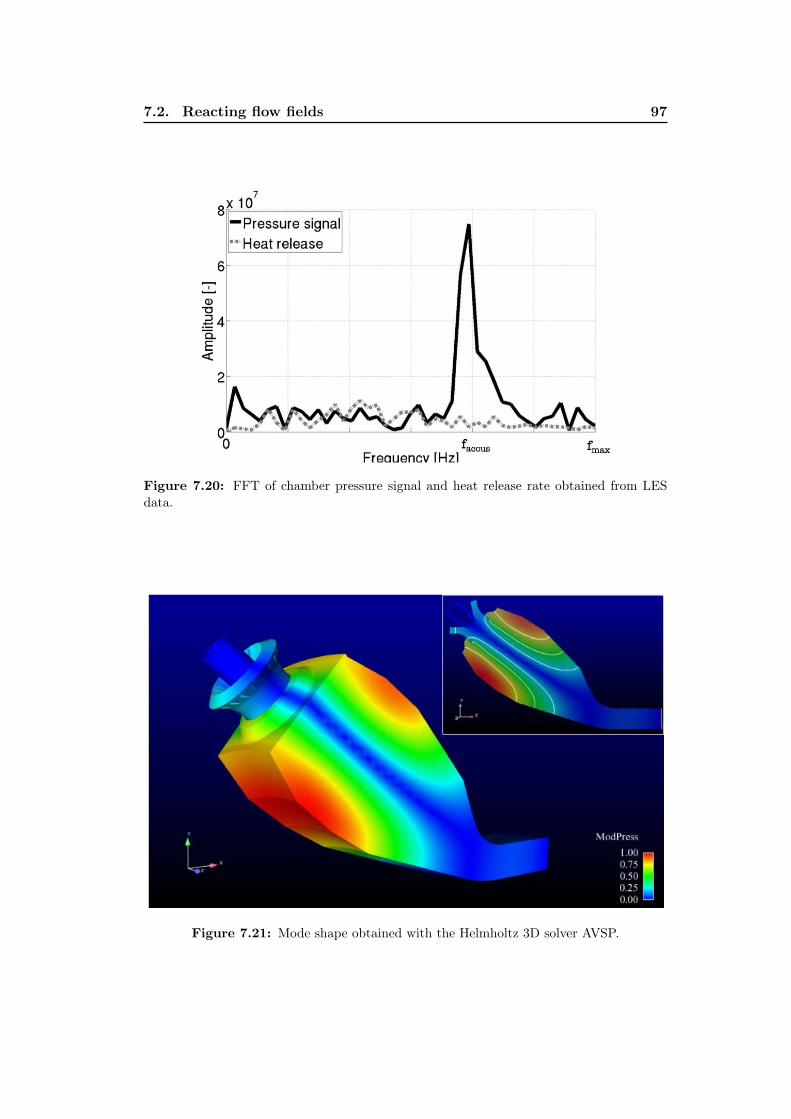
7.2. Reacting flow fields 97
Figure 7.20: FFT of chamber pressure signal and heat release rate obtained from LESdata.
Figure 7.21: Mode shape obtained with the Helmholtz 3D solver AVSP.

98 Chapter 7. Numerical results for the unforced flame
direction and its length is slightly shorter. All cases burn at a similar equivalenceratio. Acoustic analysis reveals that the first transverse eigenmode of the chamberappears in the LES while it is not seen in the real full machine. Nevertheless FFTshows that this mode does not affect the flame dynamics so that FTFs can still bemeasured using LES of a single sector.
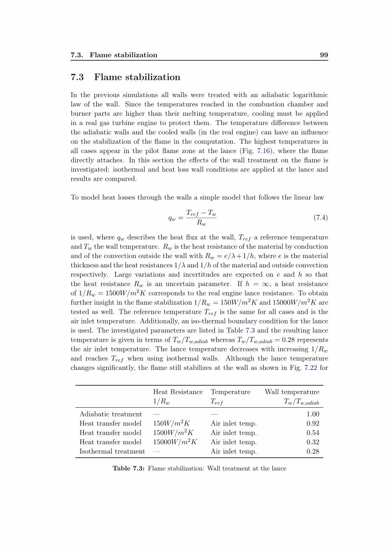
7.3. Flame stabilization 99
7.3 Flame stabilization
In the previous simulations all walls were treated with an adiabatic logarithmiclaw of the wall. Since the temperatures reached in the combustion chamber andburner parts are higher than their melting temperature, cooling must be appliedin a real gas turbine engine to protect them. The temperature difference betweenthe adiabatic walls and the cooled walls (in the real engine) can have an influenceon the stabilization of the flame in the computation. The highest temperatures inall cases appear in the pilot flame zone at the lance (Fig. 7.16), where the flamedirectly attaches. In this section the effects of the wall treatment on the flame isinvestigated: isothermal and heat loss wall conditions are applied at the lance andresults are compared.
To model heat losses through the walls a simple model that follows the linear law
qw =Tref − Tw
Rw(7.4)
is used, where qw describes the heat flux at the wall, Tref a reference temperatureand Tw the wall temperature. Rw is the heat resistance of the material by conductionand of the convection outside the wall with Rw = e/λ+1/h, where e is the materialthickness and the heat resistances 1/λ and 1/h of the material and outside convectionrespectively. Large variations and incertitudes are expected on e and h so thatthe heat resistance Rw is an uncertain parameter. If h = ∞, a heat resistanceof 1/Rw = 1500W/m2K corresponds to the real engine lance resistance. To obtainfurther insight in the flame stabilization 1/Rw = 150W/m2K and 15000W/m2K aretested as well. The reference temperature Tref is the same for all cases and is theair inlet temperature. Additionally, an iso-thermal boundary condition for the lanceis used. The investigated parameters are listed in Table 7.3 and the resulting lancetemperature is given in terms of Tw/Tw,adiab whereas Tw/Tw,adiab = 0.28 representsthe air inlet temperature. The lance temperature decreases with increasing 1/Rwand reaches Tref when using isothermal walls. Although the lance temperaturechanges significantly, the flame still stabilizes at the wall as shown in Fig. 7.22 for
Heat Resistance Temperature Wall temperature1/Rw Tref Tw/Tw,adiab
Adiabatic treatment — — 1.00
Heat transfer model 150W/m2K Air inlet temp. 0.92
Heat transfer model 1500W/m2K Air inlet temp. 0.54
Heat transfer model 15000W/m2K Air inlet temp. 0.32
Isothermal treatment — Air inlet temp. 0.28
Table 7.3: Flame stabilization: Wall treatment at the lance
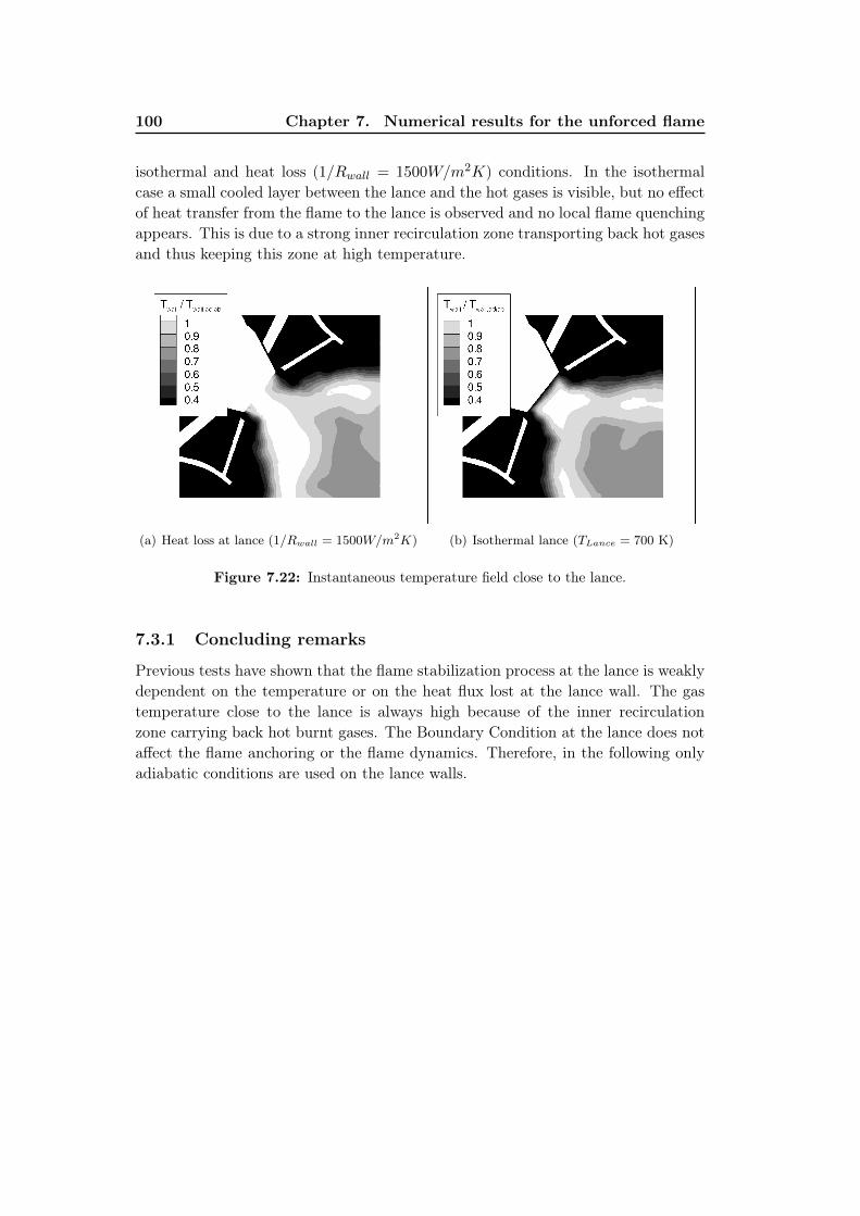
100 Chapter 7. Numerical results for the unforced flame
isothermal and heat loss (1/Rwall = 1500W/m2K) conditions. In the isothermalcase a small cooled layer between the lance and the hot gases is visible, but no effectof heat transfer from the flame to the lance is observed and no local flame quenchingappears. This is due to a strong inner recirculation zone transporting back hot gasesand thus keeping this zone at high temperature.
(a) Heat loss at lance (1/Rwall = 1500W/m2K) (b) Isothermal lance (TLance = 700 K)
Figure 7.22: Instantaneous temperature field close to the lance.
7.3.1 Concluding remarks
Previous tests have shown that the flame stabilization process at the lance is weaklydependent on the temperature or on the heat flux lost at the lance wall. The gastemperature close to the lance is always high because of the inner recirculationzone carrying back hot burnt gases. The Boundary Condition at the lance does notaffect the flame anchoring or the flame dynamics. Therefore, in the following onlyadiabatic conditions are used on the lance walls.

7.4. Bi-stable behaviour of the reacting flow 101
7.4 Bi-stable behaviour of the reacting flow
During the initialisation of the operating condition at an ambient temperature of−15◦C, LES revealed that when the transition between the two states (15◦C to-15◦C) is applied harshly, the flame detaches from the lance and a PVC develops,preventing the flame to move back to its normal stabilization point. Figure. 7.23(a)and Fig. 7.23(b) use a low pressure iso-surface to represent the PVC and a temper-ature iso-line of T/Tmean = 1.3 to track the flame surface in 2D for the attachedand detached flame respectively. In the attached case no PVC is present whereasthe detached flame features a "finger-like" rotating structure in the inner regionaround which the PVC is turning (Fig. 7.23). A similar phenomenon was observedby Staffelbach [164] who discovered that the flame detaches with decreasing fuelmass flow rate at the lance. Field tests performed by Ansaldo also showed differ-ent pressure oscillation levels depending on transition between different operatingconditions, suggesting hysteresis phenomena. The detached flame exhibits strongerpressure levels than the attached one and this is not desirable for flame stabilizationand thermo-acoustic stability. In the following section the detached flame is ana-lyzed in detail. For simplicity reasons the nomenclature listed in Table 7.4 is used.Although this arises for both burner outlets, only the CBO case will be investigatedsince both cases behave similarly.
A first impression is obtained by plotting the three-dimensional surface of the
-15CBO Attached flame-15CBO-D Detached flame
Table 7.4: Nomenclature for attached and detached flame.
averaged flame as shown in Fig. 7.24 where the flame surface is visualized by a tem-perature iso-surface (T/Tmean = 1.3) coloured by the axial velocity. The flame findstwo different stable positions for the same regime and is therefore bi-stable.
A cut through the middle plane reveals differences in the heat release field be-tween both flames which is shown in Fig. 7.25(b). Since the flame is detached fromthe lance, the high temperature region around the pilot injection disappears. In thiscase the inner recirculation zone does not reach the lance (Fig. 7.25(a)) and doesnot bring the flame back to the lance. Furthermore the attached flame acts like ageometrical contraction at the outlet of the burner accelerating the flow and leadingto higher axial velocities than in the case with detached flame. This is illustratedby plotting the axial velocity along the cuts (Fig. 7.11) in Fig. 7.26. Both flamesstill agree well in terms of position of lows and peaks but the attached flame showssignificantly higher velocities in the peaks all along the flame region (cut 2 to 7).The detached flame shows positive axial velocity in the inner region close to the
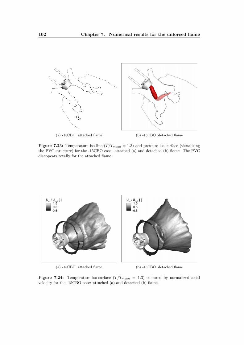
102 Chapter 7. Numerical results for the unforced flame
(a) -15CBO: attached flame (b) -15CBO: detached flame
Figure 7.23: Temperature iso-line (T/Tmean = 1.3) and pressure iso-surface (visualizingthe PVC structure) for the -15CBO case: attached (a) and detached (b) flame. The PVCdisappears totally for the attached flame.
(a) -15CBO: attached flame (b) -15CBO: detached flame
Figure 7.24: Temperature iso-surface (T/Tmean = 1.3) coloured by normalized axialvelocity for the -15CBO case: attached (a) and detached (b) flame.
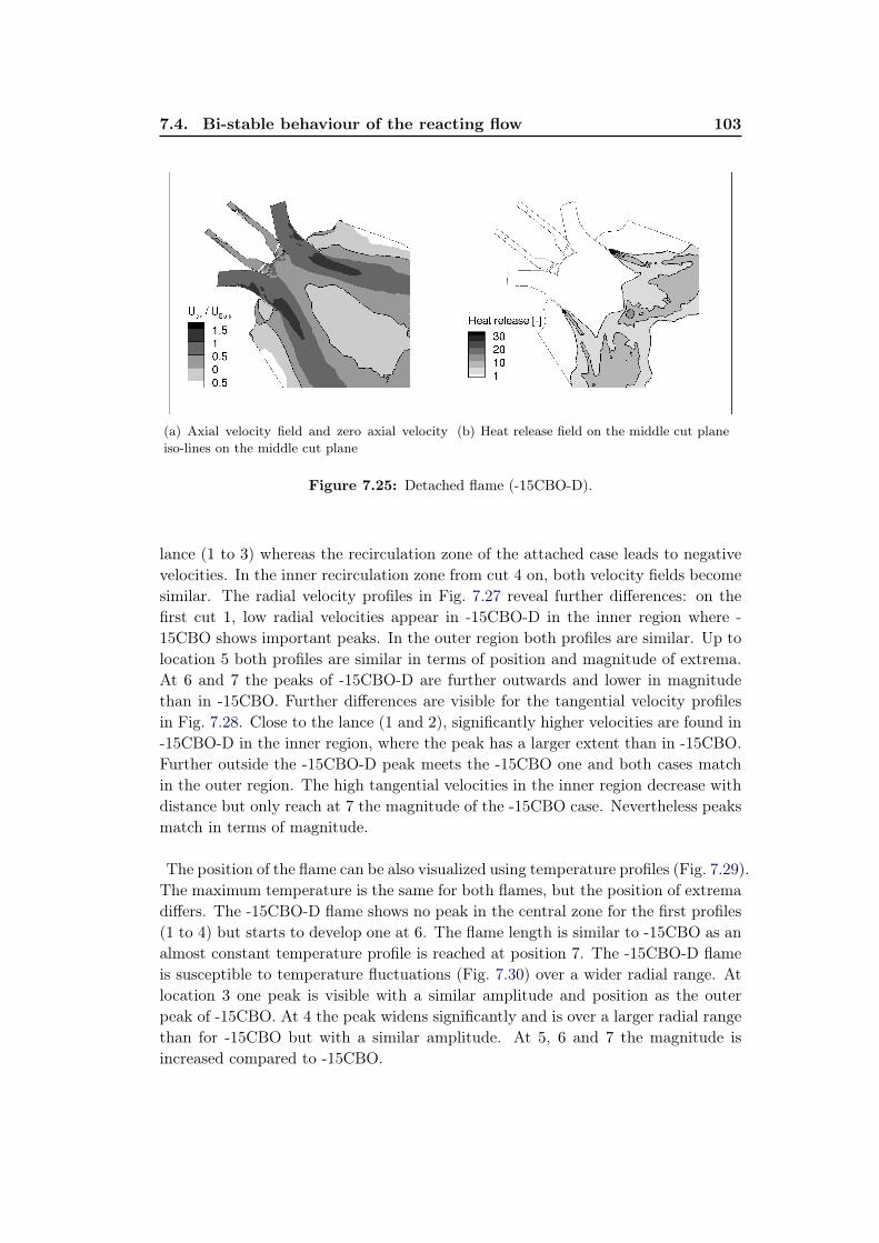
7.4. Bi-stable behaviour of the reacting flow 103
(a) Axial velocity field and zero axial velocityiso-lines on the middle cut plane
(b) Heat release field on the middle cut plane
Figure 7.25: Detached flame (-15CBO-D).
lance (1 to 3) whereas the recirculation zone of the attached case leads to negativevelocities. In the inner recirculation zone from cut 4 on, both velocity fields becomesimilar. The radial velocity profiles in Fig. 7.27 reveal further differences: on thefirst cut 1, low radial velocities appear in -15CBO-D in the inner region where -15CBO shows important peaks. In the outer region both profiles are similar. Up tolocation 5 both profiles are similar in terms of position and magnitude of extrema.At 6 and 7 the peaks of -15CBO-D are further outwards and lower in magnitudethan in -15CBO. Further differences are visible for the tangential velocity profilesin Fig. 7.28. Close to the lance (1 and 2), significantly higher velocities are found in-15CBO-D in the inner region, where the peak has a larger extent than in -15CBO.Further outside the -15CBO-D peak meets the -15CBO one and both cases matchin the outer region. The high tangential velocities in the inner region decrease withdistance but only reach at 7 the magnitude of the -15CBO case. Nevertheless peaksmatch in terms of magnitude.
The position of the flame can be also visualized using temperature profiles (Fig. 7.29).The maximum temperature is the same for both flames, but the position of extremadiffers. The -15CBO-D flame shows no peak in the central zone for the first profiles(1 to 4) but starts to develop one at 6. The flame length is similar to -15CBO as analmost constant temperature profile is reached at position 7. The -15CBO-D flameis susceptible to temperature fluctuations (Fig. 7.30) over a wider radial range. Atlocation 3 one peak is visible with a similar amplitude and position as the outerpeak of -15CBO. At 4 the peak widens significantly and is over a larger radial rangethan for -15CBO but with a similar amplitude. At 5, 6 and 7 the magnitude isincreased compared to -15CBO.

104 Chapter 7. Numerical results for the unforced flame
−2 0 2−1
−0.8
−0.6
−0.4
−0.2
0
0.2
0.4
0.6
0.8
1
y/y
ma
x [
−]
1
−2 0 2
2
−2 0 2
3
−2 0 2
Uax
/Ubulk
[−]
4
−2 0 2
5
−2 0 2
6
−2 0 2
7
−15CBO
−15CBO−D
Figure 7.26: Axial velocity profiles for the attached (-15CBO) and detached (-15CBO-D)flame.
−1 0 1−1
−0.8
−0.6
−0.4
−0.2
0
0.2
0.4
0.6
0.8
1
y/y
ma
x [
−]
1
−1 0 1
2
−1 0 1
3
−1 0 1
Urad
/Ubulk
[−]
4
−1 0 1
5
−1 0 1
6
−1 0 1
7
−15CBO
−15CBO−D
Figure 7.27: Radial velocity profiles for the attached (-15CBO) and detached (-15CBO-D)flame.
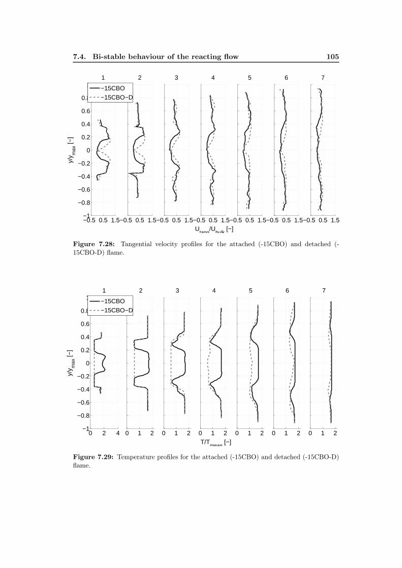
7.4. Bi-stable behaviour of the reacting flow 105
−0.5 0.5 1.5−1
−0.8
−0.6
−0.4
−0.2
0
0.2
0.4
0.6
0.8
1
y/y
ma
x [
−]
1
−0.5 0.5 1.5
2
−0.5 0.5 1.5
3
−0.5 0.5 1.5
Utang
/Ubulk
[−]
4
−0.5 0.5 1.5
5
−0.5 0.5 1.5
6
−0.5 0.5 1.5
7
−15CBO
−15CBO−D
Figure 7.28: Tangential velocity profiles for the attached (-15CBO) and detached (-15CBO-D) flame.
0 2 4−1
−0.8
−0.6
−0.4
−0.2
0
0.2
0.4
0.6
0.8
1
y/y
ma
x [
−]
1
0 1 2
2
0 1 2
3
0 1 2
T/Tmean
[−]
4
0 1 2
5
0 1 2
6
0 1 2
7
−15CBO
−15CBO−D
Figure 7.29: Temperature profiles for the attached (-15CBO) and detached (-15CBO-D)flame.
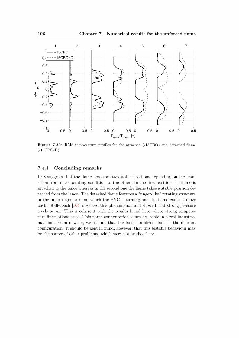
106 Chapter 7. Numerical results for the unforced flame
0 0.5−1
−0.8
−0.6
−0.4
−0.2
0
0.2
0.4
0.6
0.8
1
y/y
ma
x [
−]
1
0 0.5
2
0 0.5
3
0 0.5
TRMS
/Tmean
[−]
4
0 0.5
5
0 0.5
6
0 0.5
7
−15CBO
−15CBO−D
Figure 7.30: RMS temperature profiles for the attached (-15CBO) and detached flame(-15CBO-D)
7.4.1 Concluding remarks
LES suggests that the flame possesses two stable positions depending on the tran-sition from one operating condition to the other. In the first position the flame isattached to the lance whereas in the second one the flame takes a stable position de-tached from the lance. The detached flame features a "finger-like" rotating structurein the inner region around which the PVC is turning and the flame can not moveback. Staffelbach [164] observed this phenomenon and showed that strong pressurelevels occur. This is coherent with the results found here where strong tempera-ture fluctuations arise. This flame configuration is not desirable in a real industrialmachine. From now on, we assume that the lance-stabilized flame is the relevantconfiguration. It should be kept in mind, however, that this bistable behaviour maybe the source of other problems, which were not studied here.

7.5. Quality of the LES 107
7.5 Quality of the LES
One goal of the present thesis is to evaluate the quality of LES of complex configura-tions in an industrial context which requires limited time and computational costs.The quality of the mesh is evaluated in Fig. 7.31 and 7.32 showing the thickeningfactor for the flame and the turbulent viscosity ratio for +15CBO. The thickeningreaches its maximal value at the flame tip and is always less than 300. The PDFof the thickening factor (Fig. 7.33) shows that most of the flame is thickened witha value lower than 10 and only a few points are thickened with values around 300
(Fig. 7.33(b)). Also a reasonable ratio between turbulent and laminar viscosity isreached with maximal values downstream of the burner outlet of 500 where the meshbecomes coarse (Fig. 7.32).
At the operating pressure, the typical flame thickness of a stoechiometric flame
Figure 7.31: Thickening factor on the middle cut plane (+15CBO).
Figure 7.32: Turbulent viscosity ratio on the middle cut plane (+15CBO).
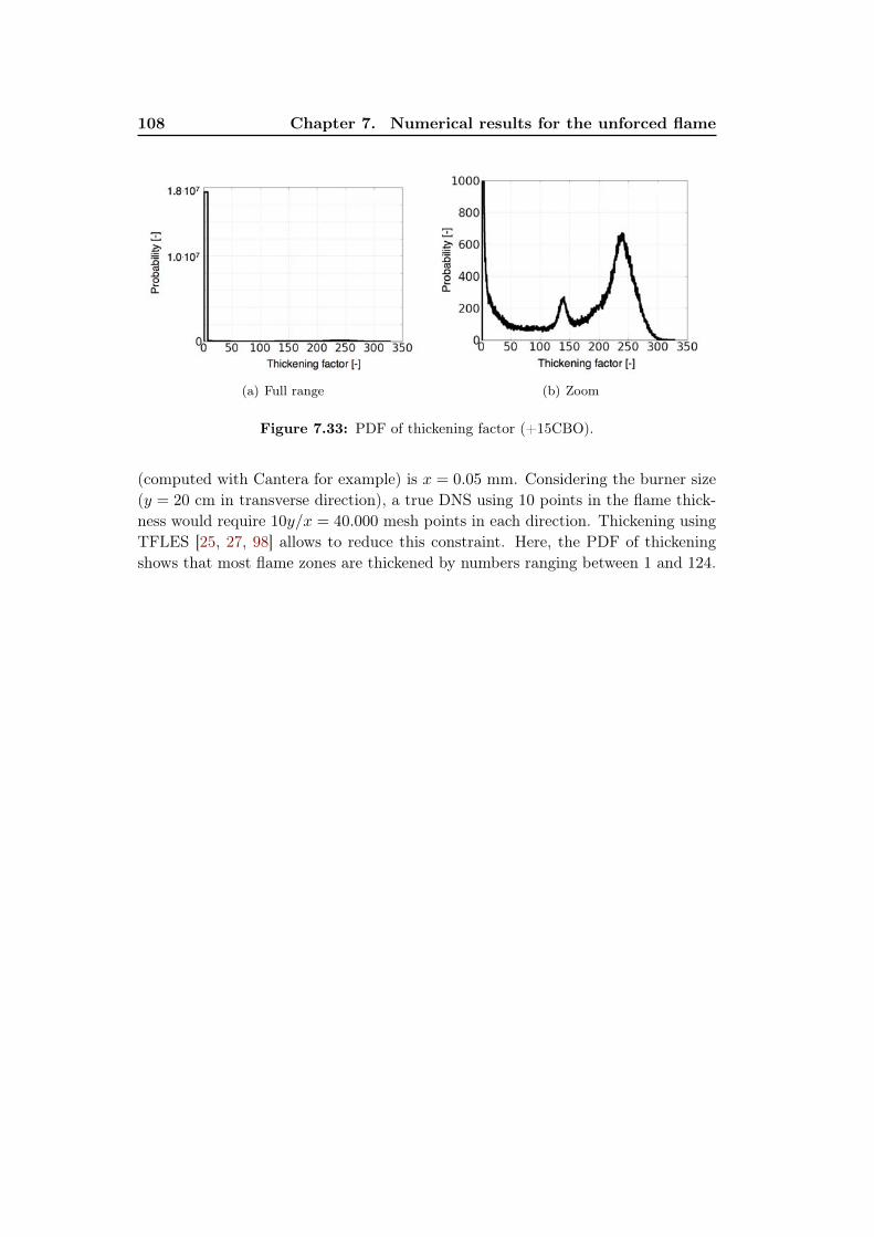
108 Chapter 7. Numerical results for the unforced flame
(a) Full range (b) Zoom
Figure 7.33: PDF of thickening factor (+15CBO).
(computed with Cantera for example) is x = 0.05 mm. Considering the burner size(y = 20 cm in transverse direction), a true DNS using 10 points in the flame thick-ness would require 10y/x = 40.000 mesh points in each direction. Thickening usingTFLES [25, 27, 98] allows to reduce this constraint. Here, the PDF of thickeningshows that most flame zones are thickened by numbers ranging between 1 and 124.
Chapter 8
Acoustically perturbed flame
Contents8.1 Pulsation procedure and system identification . . . . . . . . 112
8.1.1 Pulsation procedure . . . . . . . . . . . . . . . . . . . . . . . 1128.1.2 System identification . . . . . . . . . . . . . . . . . . . . . . . 113
8.2 Flame Transfer Function . . . . . . . . . . . . . . . . . . . . . 1148.2.1 Comparison of the identification methods . . . . . . . . . . . 116
8.3 Influence of operating conditions and burner outlets . . . . 1188.3.1 Mean pulsated flow fields . . . . . . . . . . . . . . . . . . . . 1188.3.2 Dynamic flame response . . . . . . . . . . . . . . . . . . . . . 1228.3.3 Local comparison of FTF . . . . . . . . . . . . . . . . . . . . 1228.3.4 Effect of mixture and swirl perturbation . . . . . . . . . . . . 1238.3.5 Concluding remarks . . . . . . . . . . . . . . . . . . . . . . . 126
8.4 Effects of forcing frequencies . . . . . . . . . . . . . . . . . . . 1298.4.1 Dynamic flame response . . . . . . . . . . . . . . . . . . . . . 1298.4.2 Local comparison of FTF . . . . . . . . . . . . . . . . . . . . 1298.4.3 Effects of fuel heterogeneities and swirl perturbation . . . . . 1328.4.4 Concluding remarks . . . . . . . . . . . . . . . . . . . . . . . 140
Modern regulation policies on pollutant emissions lead to lean (technically) pre-mixed combustion systems [97]. These low-emission gas turbines are known to beparticularly susceptible to thermo-acoustic instabilities [126] and their predictionhas become an important task today to prevent the appearance of acoustically cou-pled instabilities at an early design stage [74, 86, 189]. For acoustically compactflames, a common approach can be found in the literature and was first introducedby Crocco [29, 30]. In this approach, the Flame Transfer Function (FTF) is the keyparameter and is defined as the ratio of the relative heat release fluctuation (q/q)to the relative inlet velocity perturbation (u/u) issued by the acoustic field. In thefrequency domain it writes
F (ω) =q/q
u/u. (8.1)
with ω being the angular frequency.
The FTF is affected by different mechanisms acting simultaneously on the heatrelease rate fluctuation and therefore difficult to isolate [178]:

110 Chapter 8. Acoustically perturbed flame
• The axial velocity perturbation:Flame Transfer Functions have been extensively studied in laminar and tur-bulent premixed flames where only the axial velocity perturbation is at play.Investigations of laminar conical flames performed by Karimi et al. [76], in-verted conical by Durox et al. [38] and multi-slit conical flames studied byKornilov et al. [85] revealed that the FTF gain shows a low-pass filter be-haviour. Schuller et al. [150] observed from laminar flames and Armittage etal. [2] from turbulent V-flames, an overshoot in gain and associated this tovortex roll-up at the flame base. The phase φ of the FTF evolves in thesecases in an almost linear way with the frequency f indicating that axial veloc-ity perturbations propagate convectively from the burner outlet to the flame,thereby controlling the delay τ of the FTF: τ = φ/(2πf).
• The perturbation of swirl:Among the recent contributions towards the understanding of the mechanismsat play for swirled flames, the importance of swirl number fluctuations has beenclearly identified. Straub and Richards [173] first noticed a strong impact ofthe swirler position on the combustion oscillations. Hirsch et al. [59] henceinvestigated the effect of swirler designs and found that an additional timelag is responsible for changes in the FTF. Komarek et al. [84] investigated theinfluence of several swirler positions on the FTF and concluded that distur-bances propagate at a convective and an acoustic speed downstream of theswirler position. Finally, Palies et al. [117, 119] have shown that the acous-tic perturbations reaching the swirler generate transverse velocity fluctuationswhich are convected by the flow.
• The perturbation of mixture:Since most gas turbines are partially premixed, fluctuations of equivalenceratio may also modify their flame response [104]. Schuermans et al. [148]compared the measured transfer matrix of a turbulent flame for a technicallypremixed and a fully premixed system and found the maximal value in am-plitude to increase for the technically premixed case where equivalence ratioperturbations are present. Kim et al. [82] found a phase difference betweenequivalence ratio and velocity at the combustor inlet suggesting that this phasedetermines if both effects cancel out or amplify the dynamic flame response.Furthermore, they showed that this phase difference is a function of frequency,fuel injection location, fuel injector impedance and the mean velocity in thenozzle.
These mechanisms have been studied for simple laboratory premixed flames butmuch less information is available for real gas turbines. This point is investigatedhere using LES of a real burner. Thanks to this fully unsteady numerical approach,effects of mass flow rate perturbation, mixture fluctuation and swirl number pertur-bation can be studied.
111
This chapter is organized as follows: first (section 8.1) the specific informationfor the pulsation of the different cases are given and the methodology is shortlysummarized (see chapter 3 for more a detailed description). Then the Flame TransferFunctions of the cases with different operating conditions and burner outlets aregiven and differences are discussed (section 8.2). Then the specifications of theFTFs are analyzed in detail for the single forcing frequency which allows to obtainfurther insight into the mechanisms influencing the dynamic response of the flame .Therefore the differences due to operating conditions and burner outlets are furtherevaluated at one specific frequency (section 8.3) and one case is analyzed for severalfrequencies (section 8.4). Further effects such as axial velocity perturbation, swirlfluctuation and mixing inhomogeneities are considered. Finally, additional LESare performed separating the effect of mixing inhomogeneities (section 9.1) and ofvelocity perturbation (section 9.2) on the FTF.
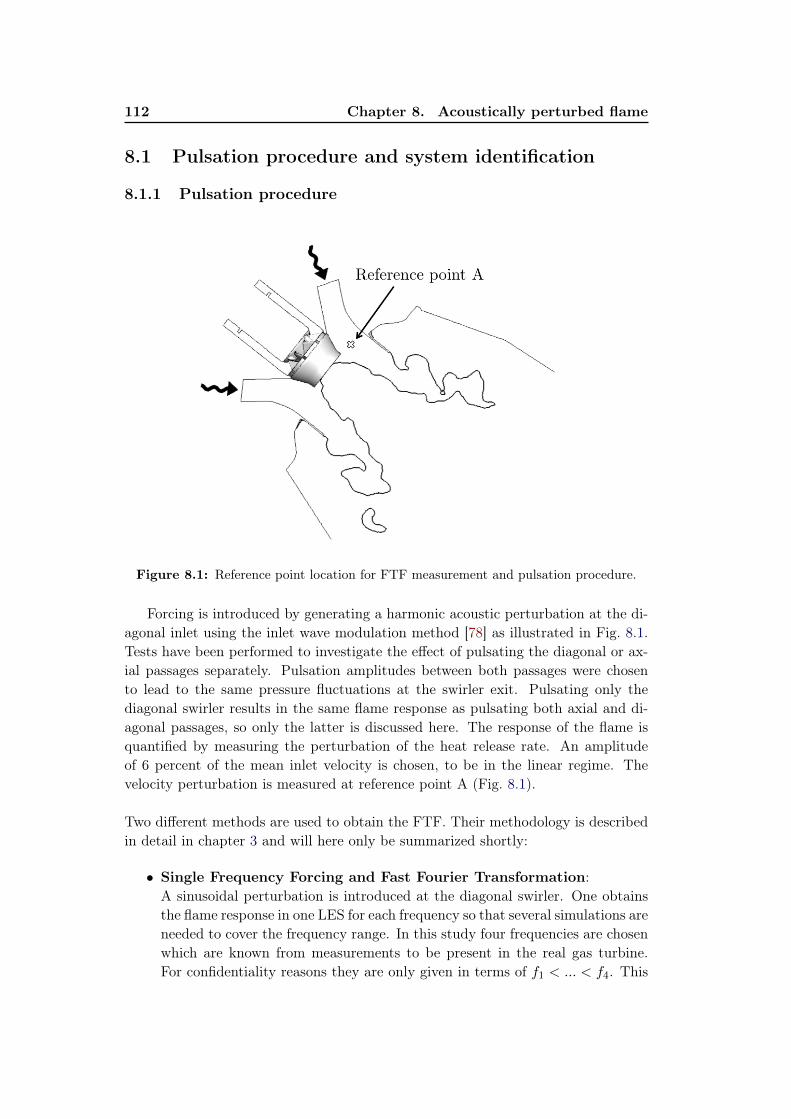
112 Chapter 8. Acoustically perturbed flame
8.1 Pulsation procedure and system identification
8.1.1 Pulsation procedure
Figure 8.1: Reference point location for FTF measurement and pulsation procedure.
Forcing is introduced by generating a harmonic acoustic perturbation at the di-agonal inlet using the inlet wave modulation method [78] as illustrated in Fig. 8.1.Tests have been performed to investigate the effect of pulsating the diagonal or ax-ial passages separately. Pulsation amplitudes between both passages were chosento lead to the same pressure fluctuations at the swirler exit. Pulsating only thediagonal swirler results in the same flame response as pulsating both axial and di-agonal passages, so only the latter is discussed here. The response of the flame isquantified by measuring the perturbation of the heat release rate. An amplitudeof 6 percent of the mean inlet velocity is chosen, to be in the linear regime. Thevelocity perturbation is measured at reference point A (Fig. 8.1).
Two different methods are used to obtain the FTF. Their methodology is describedin detail in chapter 3 and will here only be summarized shortly:
• Single Frequency Forcing and Fast Fourier Transformation:A sinusoidal perturbation is introduced at the diagonal swirler. One obtainsthe flame response in one LES for each frequency so that several simulations areneeded to cover the frequency range. In this study four frequencies are chosenwhich are known from measurements to be present in the real gas turbine.For confidentiality reasons they are only given in terms of f1 < ... < f4. This
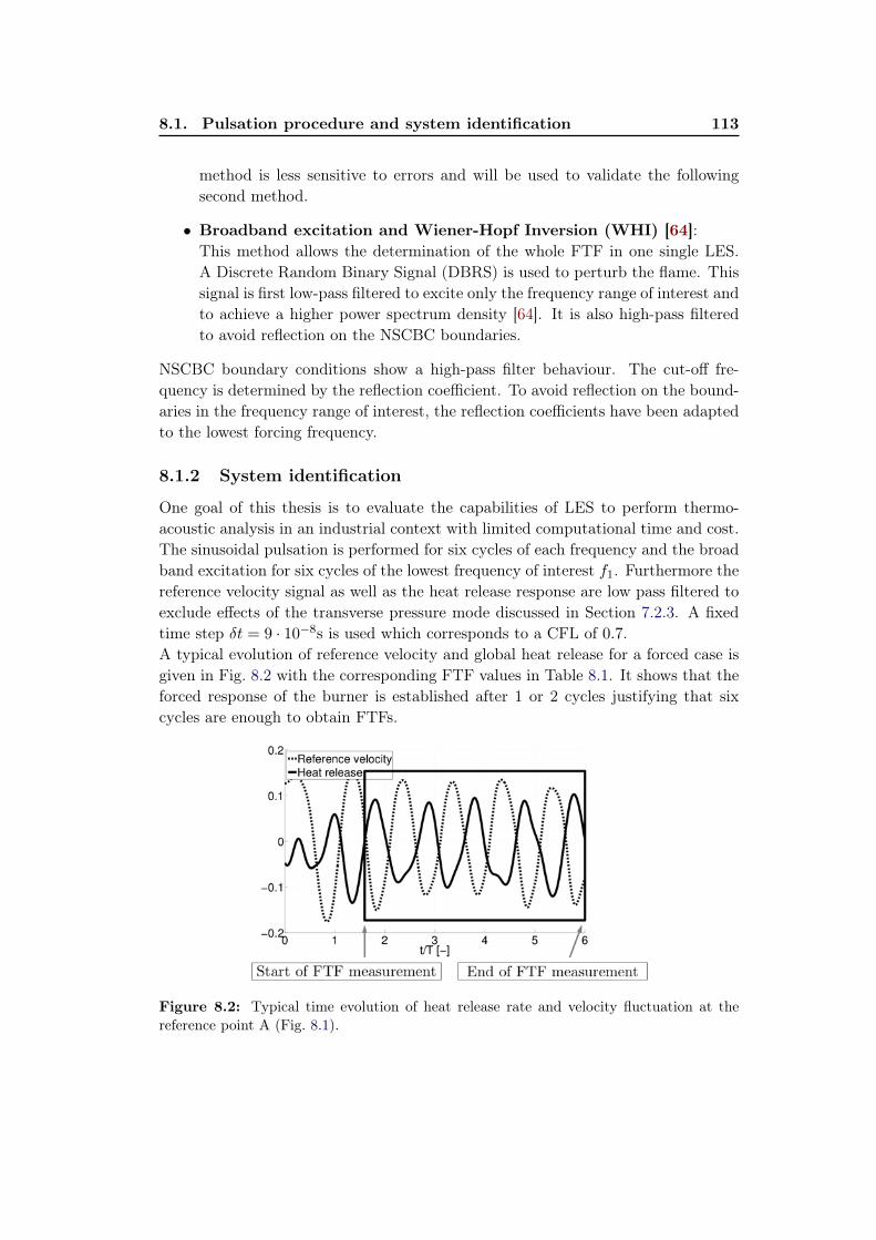
8.1. Pulsation procedure and system identification 113
method is less sensitive to errors and will be used to validate the followingsecond method.
• Broadband excitation and Wiener-Hopf Inversion (WHI) [64]:This method allows the determination of the whole FTF in one single LES.A Discrete Random Binary Signal (DBRS) is used to perturb the flame. Thissignal is first low-pass filtered to excite only the frequency range of interest andto achieve a higher power spectrum density [64]. It is also high-pass filteredto avoid reflection on the NSCBC boundaries.
NSCBC boundary conditions show a high-pass filter behaviour. The cut-off fre-quency is determined by the reflection coefficient. To avoid reflection on the bound-aries in the frequency range of interest, the reflection coefficients have been adaptedto the lowest forcing frequency.
8.1.2 System identification
One goal of this thesis is to evaluate the capabilities of LES to perform thermo-acoustic analysis in an industrial context with limited computational time and cost.The sinusoidal pulsation is performed for six cycles of each frequency and the broadband excitation for six cycles of the lowest frequency of interest f1. Furthermore thereference velocity signal as well as the heat release response are low pass filtered toexclude effects of the transverse pressure mode discussed in Section 7.2.3. A fixedtime step δt = 9 · 10−8s is used which corresponds to a CFL of 0.7.A typical evolution of reference velocity and global heat release for a forced case isgiven in Fig. 8.2 with the corresponding FTF values in Table 8.1. It shows that theforced response of the burner is established after 1 or 2 cycles justifying that sixcycles are enough to obtain FTFs.
Figure 8.2: Typical time evolution of heat release rate and velocity fluctuation at thereference point A (Fig. 8.1).
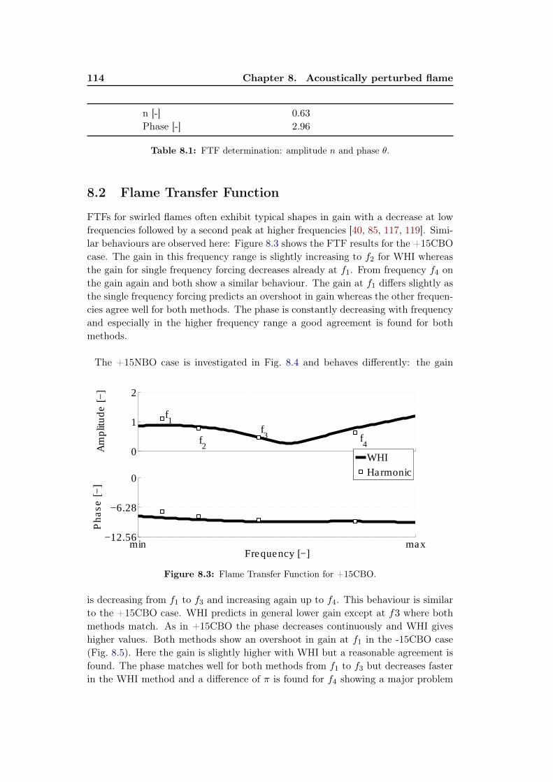
114 Chapter 8. Acoustically perturbed flame
n [-] 0.63
Phase [-] 2.96
Table 8.1: FTF determination: amplitude n and phase θ.
8.2 Flame Transfer Function
FTFs for swirled flames often exhibit typical shapes in gain with a decrease at lowfrequencies followed by a second peak at higher frequencies [40, 85, 117, 119]. Simi-lar behaviours are observed here: Figure 8.3 shows the FTF results for the +15CBOcase. The gain in this frequency range is slightly increasing to f2 for WHI whereasthe gain for single frequency forcing decreases already at f1. From frequency f4 onthe gain again and both show a similar behaviour. The gain at f1 differs slightly asthe single frequency forcing predicts an overshoot in gain whereas the other frequen-cies agree well for both methods. The phase is constantly decreasing with frequencyand especially in the higher frequency range a good agreement is found for bothmethods.
The +15NBO case is investigated in Fig. 8.4 and behaves differently: the gain
0
1
2
f1
f2
f3 f
4
Am
plit
ud
e [
−]
min max−12.56
−6.28
0
Frequency [−]
Ph
ase
[−
]
WHI
Harmonic
Figure 8.3: Flame Transfer Function for +15CBO.
is decreasing from f1 to f3 and increasing again up to f4. This behaviour is similarto the +15CBO case. WHI predicts in general lower gain except at f3 where bothmethods match. As in +15CBO the phase decreases continuously and WHI giveshigher values. Both methods show an overshoot in gain at f1 in the -15CBO case(Fig. 8.5). Here the gain is slightly higher with WHI but a reasonable agreement isfound. The phase matches well for both methods from f1 to f3 but decreases fasterin the WHI method and a difference of π is found for f4 showing a major problem

8.2. Flame Transfer Function 115
0
1
2A
mp
litu
de
[−
]
min max−12.56
−6.28
0
Frequency [−]
Ph
ase
[−
]
WHI
Harmonic
Figure 8.4: Flame Transfer Function for +15NBO.
for WHI at this frequency. The -15NBO case in Fig. 8.6 shows as all cases a peak
0
1
2
Am
plit
ud
e [
−]
min max−12.56
−6.28
0
Frequency [−]
Ph
ase
[−
]
WHI
Harmonic
Figure 8.5: Flame Transfer Function for -15CBO.
at f1, decreases until f3 and increases again for the harmonic forcing. The phasedecreases with frequency and corresponds to the other cases. The gain agrees wellbetween WHI and harmonic forcing, whereas WHI predicts a higher phase.
Note that for all cases the minimal frequency shown here do not correspond tofmin = 0 since the multi-frequential signal has also been high-pass filtered in orderto avoid reflections at the boundaries for low frequencies and results for f < fminare not physical. Following [127] an amplitude n(f = 0) = 1 is expected. The FlameTransfer Functions exhibit typical behaviour in all cases. The phase decreases with

116 Chapter 8. Acoustically perturbed flame
0
1
2
Am
plit
ud
e [
−]
min max−12.56
−6.28
0
Frequency [−]
Ph
ase
[−
]
WHI
Harmonic
Figure 8.6: Flame Transfer Function for -15NBO.
increasing frequency and the gain is characterized by at least two zones of largeramplification. Concerning the gain, both CBO cases show an overshoot in gain atf1, decreasing to f3 and increasing again. The NBO cases agree as well in terms ofgain with a peak at f1 which is below 1 and a similar behaviour as the CBO caseswith decreasing and increasing gain. The phase is generally decreasing but a variabletime lag is found in all cases. Comparing the CBO cases with the NBO cases showsthat most frequencies lead to a shorter time delay for the CBO case. This resultis contradictory to what is found in literature: Krebs et al. state in [103] that thetime lag increases when adding a CBO compared to the case with no CBO. Theirresult has been obtained by postprocessing CFD RANS data and the applicationof the Rayleigh criterion showed an improvement of thermoacoustic stability whichhas been validated against field tests [8]. This stands in contradiction to what isfound here: the CBO cases show shorter time lags at both operating conditions.
8.2.1 Comparison of the identification methods
For all cases a reasonable agreement is found between the two methods WHI andHarmonic but some differences occur especially at high frequencies. They can partlybe explained by the complexity of the WHI method and its sensitivity to errors.Another source of error is that the velocity signal is taken at a reference point (seeFig. 8.1) where turbulent fluctuations can have an influence. This is easy to recog-nize and to filter for an harmonic excitation but it becomes more complicated with arandom signal. Furthermore, Huber [64] states that even with a low signal to noiseratio of S/N = 4 the quality of the identification process is 90% when having atotal simulation time of ten times the longest time lag considered. Below ten timesthe quality decreases drastically. Here, the WHI simulation was performed to bein the quality range of > 90% but this means also that some errors are expected.
8.2. Flame Transfer Function 117
Generally, the Fast Fourier Transformation is less sensitive to errors in the systemidentification process than the WHI method. Additionally it allows to easily sep-arate turbulence effects from those coming from the excitation. Although WHI issupposed to minimize the error in a least mean square sense, which means to sep-arate effects from turbulence and excitation, a long time series is needed to reachstatistical convergence.
To study the dynamic flame response more in detail, in the following the FTFsobtained by harmonic excitation are analysed in order to determine which mecha-nisms are at play. In a first step the two operating conditions and burner outletswill be compared to obtain insight into the mechanisms leading to a shorter timelag for the CBO cases. Second, the response to different excitation signals will beevaluated to study the differences in gain and time delay at several frequencies.

118 Chapter 8. Acoustically perturbed flame
8.3 Influence of operating conditions and burner outlets
Constructing stability maps of a given combustor as a function of operating con-ditions (air flow rate and equivalence ratio) is a classical problem in combustion.For swirled flows, the influence of operating conditions on the stability of a leanpremixed swirl-stabilized burner has been studied experimentally for example byBroda et al. [15] and Seo [159]. They found instabilities to increase for increasedinlet air temperatures, equivalence ratios from 0.5 to 0.7 and an increase in insta-bility intensity for decreasing swirler angles. Increasing inlet velocity was foundby Venkataraman et al. [183] to increase unstable behaviour on a bluff-body stabi-lized combustor. Instability occurred for low equivalence ratios of 0.55 and aroundstoichiometry. Increasing swirl stabilizes the combustor at high equivalence ratios.Bernier et al. [7] investigated the instability mechanisms in a premixed prevaporizedcombustor. Co- and counter-rotating swirlers were used and instabilities occurredfor the first when the fuel injection velocity was less than a critical value whereas thecounter-swirl configuration triggered instability for higher injection velocities. Ad-ditionally, instabilities arised for equivalence ratios higher a threshold value whichis in contrast to the observations made in [183].
The geometry of a combustion chamber is of great importance to the stability ofthe gas turbine since it determines the flow and flame characteristics as well as theacoustic properties of the system [63]. The geometry of the combustion chamberis amongst others characterized by its dimensions in length and diameter, the fuelinjection system, inlet and exit conditions and the flame stabilization setup. Severalduct geometries were tested by Katsuki et al. [77] on a bluff-body stabilized burnerand only one configuration showed stable combustion. Straub and Richards [172]changed the fuel nozzle location along the burner axis of a lean premixed configura-tion and altered the interaction between heat release and pressure oscillations sincethe distance and thus the time lag changed.
This small literature review suggests that geometry and operating conditions changesmust affect the FTF. In this section, we investigate how a change of geometry (CBOor no CBO) or a change in regime (−15◦C or +15◦C) changes FTF in our compu-tations. The analysis between the two different operating conditions and burneroutlets is performed by means of the averaged pulsated flow fields and the dynamicsof the flame.
8.3.1 Mean pulsated flow fields
An interesting issue to study combustion instabilities is to know whether meanfields with forcing remain similar to unforced mean fields since this is an assump-tion used to linearize equations in almost all approaches [31]. This point was testedhere: averaged pulsated flow fields behave similarly in both operating conditions(-15◦C and +15◦C) compared to their averaged non-pulsated ones, so that only the

8.3. Influence of operating conditions and burner outlets 119
cases +15CBO and +15NBO are shown here. The temperature profiles along thecuts match very well for the pulsated and non-pulsated averaged flame of +15CBO(Fig. 8.7) in terms of position and magnitude extrema, meaning that both flamesare in the same averaged position. Since the stabilization of the flame is determinedby the recirculation zones, the velocity profiles agree also very well for both cases asshown in Fig. 8.8 on the axial velocity. Nevertheless, differences occur in the RMStemperature profiles (Fig. 8.9): The fluctuations are higher close to the lance (1) andreach almost the double of the non-pulsated case at cut 2. A similar behaviour isobserved for the +15NBO case. Both temperature profiles agree (Fig. 8.10) as wellas velocity profiles (not shown). The fluctuations of temperature in Fig. 8.11 revealalso differences in this case: compared to the non-pulsated case, RMS fluctuationsare about doubled in the pulsated one on the first profiles. These pulsations decreasewith downstream distance showing that the effect of forcing remains limited to thenear-swirler zone. After cut 4 typically, the flow is almost unaffected by forcing andeven RMS values are similar for forced and unforced cases.
0 1 2−1
−0.8
−0.6
−0.4
−0.2
0
0.2
0.4
0.6
0.8
1
y/y
ma
x [
−]
1
0 1 2
2
0 1 2
3
0 1 2
T/Tmean
[−]
4
0 1 2
5
0 1 2
6
0 1 2
7
Non−pulsated flame
Pulsated flame
Figure 8.7: +15CBO: Temperature profiles for the averaged pulsated and non-pulsatedflame at f4.
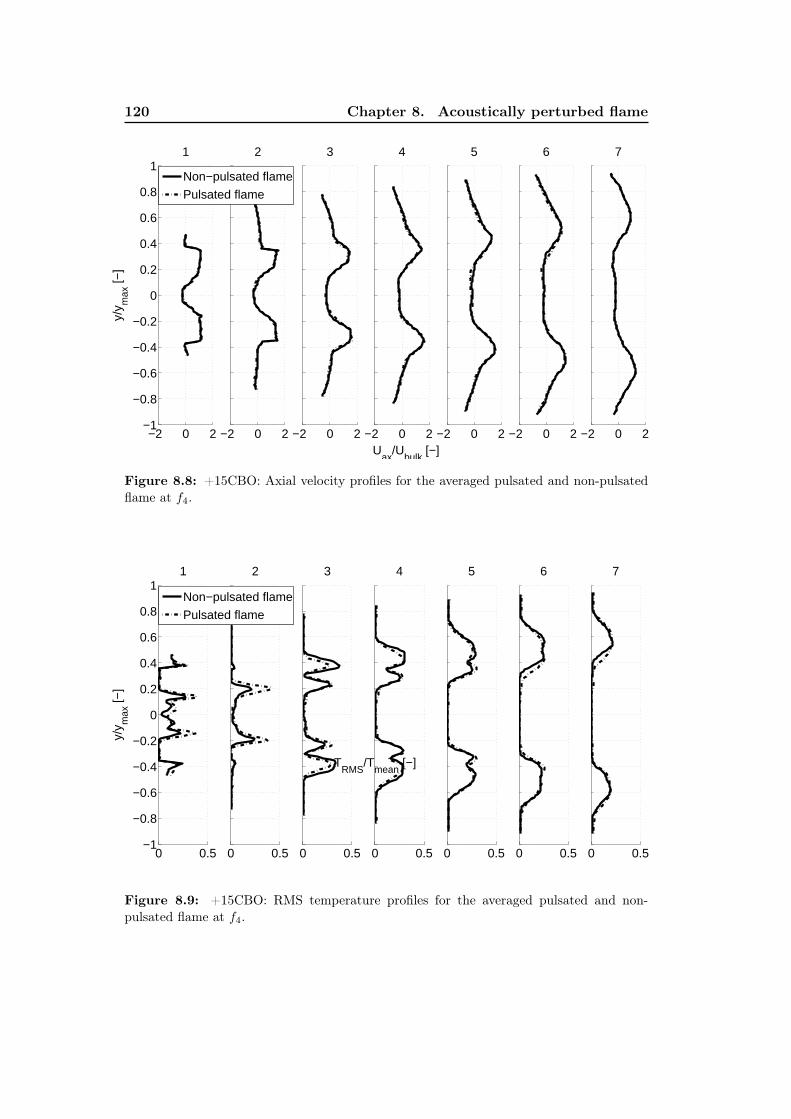
120 Chapter 8. Acoustically perturbed flame
−2 0 2−1
−0.8
−0.6
−0.4
−0.2
0
0.2
0.4
0.6
0.8
1
y/y
ma
x [
−]
1
−2 0 2
2
−2 0 2
3
−2 0 2
Uax
/Ubulk
[−]
4
−2 0 2
5
−2 0 2
6
−2 0 2
7
Non−pulsated flame
Pulsated flame
Figure 8.8: +15CBO: Axial velocity profiles for the averaged pulsated and non-pulsatedflame at f4.
0 0.5−1
−0.8
−0.6
−0.4
−0.2
0
0.2
0.4
0.6
0.8
1
y/y
ma
x [
−]
1
0 0.5
2
0 0.5
3
0 0.5
TRMS
/Tmean
[−]
4
0 0.5
5
0 0.5
6
0 0.5
7
Non−pulsated flame
Pulsated flame
Figure 8.9: +15CBO: RMS temperature profiles for the averaged pulsated and non-pulsated flame at f4.
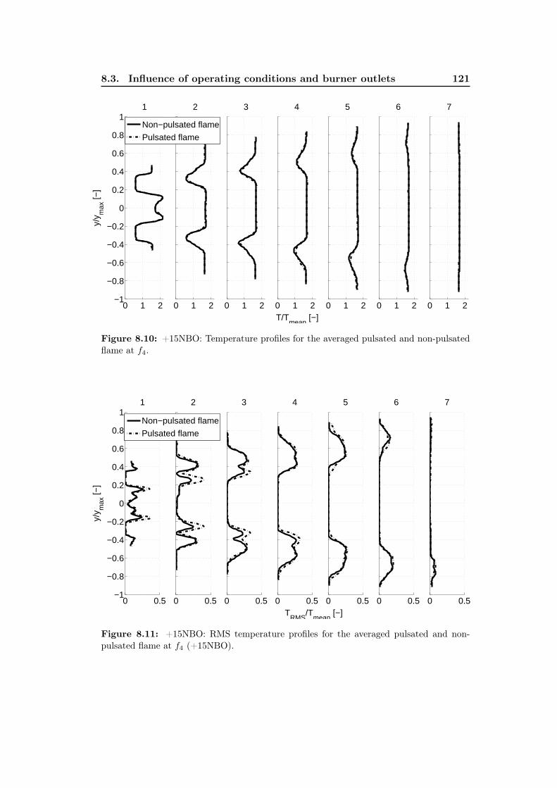
8.3. Influence of operating conditions and burner outlets 121
0 1 2−1
−0.8
−0.6
−0.4
−0.2
0
0.2
0.4
0.6
0.8
1
y/y
ma
x [
−]
1
0 1 2
2
0 1 2
3
0 1 2
T/Tmean
[−]
4
0 1 2
5
0 1 2
6
0 1 2
7
Non−pulsated flame
Pulsated flame
Figure 8.10: +15NBO: Temperature profiles for the averaged pulsated and non-pulsatedflame at f4.
0 0.5−1
−0.8
−0.6
−0.4
−0.2
0
0.2
0.4
0.6
0.8
1
y/y
ma
x [
−]
1
0 0.5
2
0 0.5
3
0 0.5
TRMS
/Tmean
[−]
4
0 0.5
5
0 0.5
6
0 0.5
7
Non−pulsated flame
Pulsated flame
Figure 8.11: +15NBO: RMS temperature profiles for the averaged pulsated and non-pulsated flame at f4 (+15NBO).
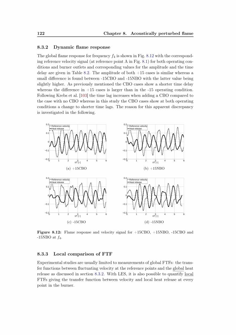
122 Chapter 8. Acoustically perturbed flame
8.3.2 Dynamic flame response
The global flame response for frequency f4 is shown in Fig. 8.12 with the correspond-ing reference velocity signal (at reference point A in Fig. 8.1) for both operating con-ditions and burner outlets and corresponding values for the amplitude and the timedelay are given in Table 8.2. The amplitude of both +15 cases is similar whereas asmall difference is found between -15CBO and -15NBO with the latter value beingslightly higher. As previously mentioned the CBO cases show a shorter time delaywhereas the difference in +15 cases is larger than in the -15 operating condition.Following Krebs et al. [103] the time lag increases when adding a CBO compared tothe case with no CBO whereas in this study the CBO cases show at both operatingconditions a change to shorter time lags. The reason for this apparent discrepancyis investigated in the following.
0 1 2 3 4 5 6−0.2
−0.1
0
0.1
0.2
t/T [−]
Reference velocityHeat release
(a) +15CBO
0 1 2 3 4 5 6−0.2
−0.1
0
0.1
0.2
t/T [−]
Reference velocityHeat release
(b) +15NBO
0 1 2 3 4 5 6−0.2
−0.1
0
0.1
0.2
t/T [−]
Reference velocityHeat release
(c) -15CBO
0 1 2 3 4 5 6−0.2
−0.1
0
0.1
0.2
t/T [−]
Reference velocityHeat release
(d) -15NBO
Figure 8.12: Flame response and velocity signal for +15CBO, +15NBO, -15CBO and-15NBO at f4.
8.3.3 Local comparison of FTF
Experimental studies are usually limited to measurements of global FTFs: the trans-fer functions between fluctuating velocity at the reference points and the global heatrelease as discussed in section 8.3.2. With LES, it is also possible to quantify localFTFs giving the transfer function between velocity and local heat release at everypoint in the burner.
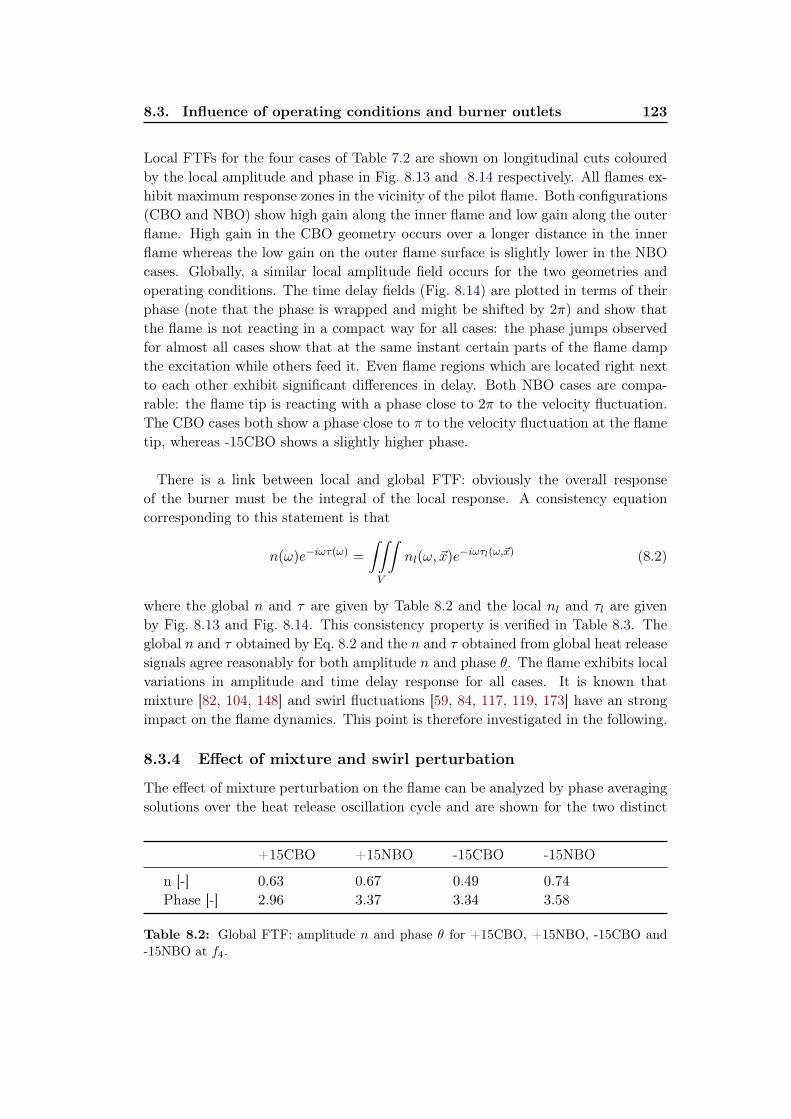
8.3. Influence of operating conditions and burner outlets 123
Local FTFs for the four cases of Table 7.2 are shown on longitudinal cuts colouredby the local amplitude and phase in Fig. 8.13 and 8.14 respectively. All flames ex-hibit maximum response zones in the vicinity of the pilot flame. Both configurations(CBO and NBO) show high gain along the inner flame and low gain along the outerflame. High gain in the CBO geometry occurs over a longer distance in the innerflame whereas the low gain on the outer flame surface is slightly lower in the NBOcases. Globally, a similar local amplitude field occurs for the two geometries andoperating conditions. The time delay fields (Fig. 8.14) are plotted in terms of theirphase (note that the phase is wrapped and might be shifted by 2π) and show thatthe flame is not reacting in a compact way for all cases: the phase jumps observedfor almost all cases show that at the same instant certain parts of the flame dampthe excitation while others feed it. Even flame regions which are located right nextto each other exhibit significant differences in delay. Both NBO cases are compa-rable: the flame tip is reacting with a phase close to 2π to the velocity fluctuation.The CBO cases both show a phase close to π to the velocity fluctuation at the flametip, whereas -15CBO shows a slightly higher phase.
There is a link between local and global FTF: obviously the overall responseof the burner must be the integral of the local response. A consistency equationcorresponding to this statement is that
n(ω)e−iωτ(ω) =
∫∫∫V
nl(ω, ~x)e−iωτl(ω,~x) (8.2)
where the global n and τ are given by Table 8.2 and the local nl and τl are givenby Fig. 8.13 and Fig. 8.14. This consistency property is verified in Table 8.3. Theglobal n and τ obtained by Eq. 8.2 and the n and τ obtained from global heat releasesignals agree reasonably for both amplitude n and phase θ. The flame exhibits localvariations in amplitude and time delay response for all cases. It is known thatmixture [82, 104, 148] and swirl fluctuations [59, 84, 117, 119, 173] have an strongimpact on the flame dynamics. This point is therefore investigated in the following.
8.3.4 Effect of mixture and swirl perturbation
The effect of mixture perturbation on the flame can be analyzed by phase averagingsolutions over the heat release oscillation cycle and are shown for the two distinct
+15CBO +15NBO -15CBO -15NBO
n [-] 0.63 0.67 0.49 0.74
Phase [-] 2.96 3.37 3.34 3.58
Table 8.2: Global FTF: amplitude n and phase θ for +15CBO, +15NBO, -15CBO and-15NBO at f4.
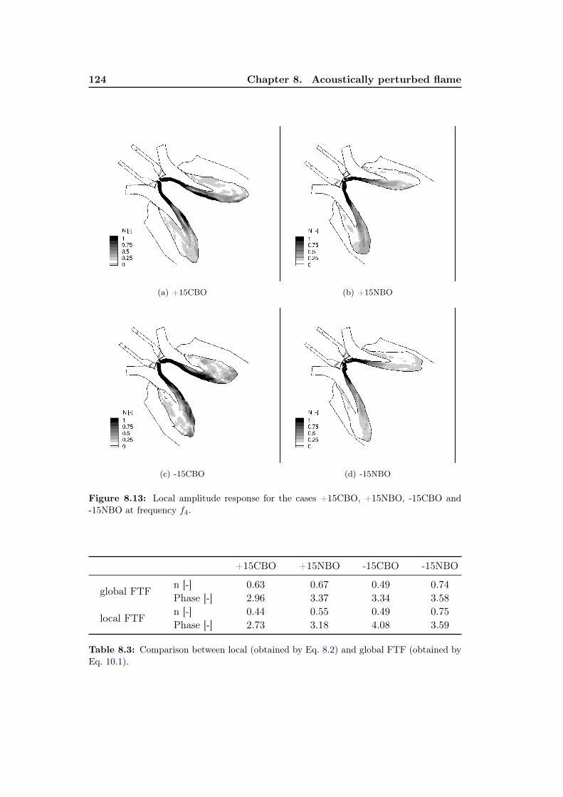
124 Chapter 8. Acoustically perturbed flame
(a) +15CBO (b) +15NBO
(c) -15CBO (d) -15NBO
Figure 8.13: Local amplitude response for the cases +15CBO, +15NBO, -15CBO and-15NBO at frequency f4.
+15CBO +15NBO -15CBO -15NBO
global FTFn [-] 0.63 0.67 0.49 0.74
Phase [-] 2.96 3.37 3.34 3.58
local FTFn [-] 0.44 0.55 0.49 0.75
Phase [-] 2.73 3.18 4.08 3.59
Table 8.3: Comparison between local (obtained by Eq. 8.2) and global FTF (obtained byEq. 10.1).

8.3. Influence of operating conditions and burner outlets 125
(a) +15CBO (b) +15NBO
(c) -15CBO (d) -15NBO
Figure 8.14: Local phase response for the cases +15CBO, +15NBO, -15CBO and -15NBOat frequency f4.
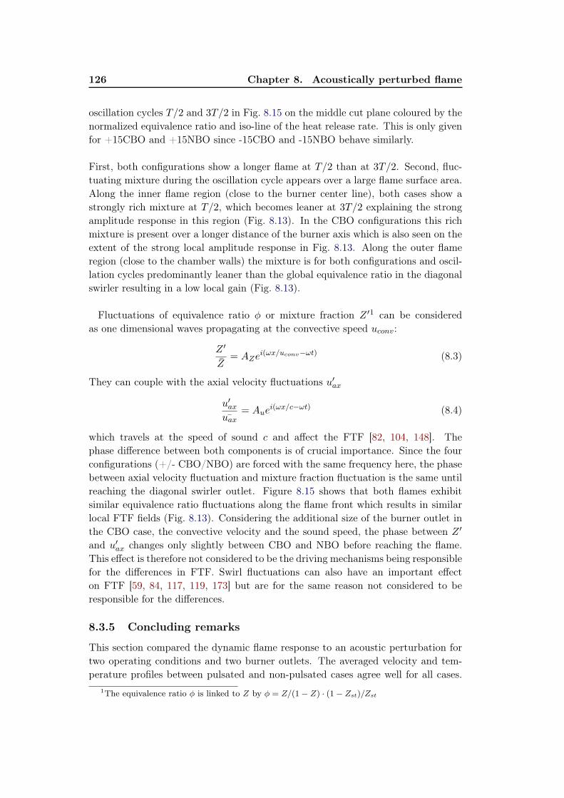
126 Chapter 8. Acoustically perturbed flame
oscillation cycles T/2 and 3T/2 in Fig. 8.15 on the middle cut plane coloured by thenormalized equivalence ratio and iso-line of the heat release rate. This is only givenfor +15CBO and +15NBO since -15CBO and -15NBO behave similarly.
First, both configurations show a longer flame at T/2 than at 3T/2. Second, fluc-tuating mixture during the oscillation cycle appears over a large flame surface area.Along the inner flame region (close to the burner center line), both cases show astrongly rich mixture at T/2, which becomes leaner at 3T/2 explaining the strongamplitude response in this region (Fig. 8.13). In the CBO configurations this richmixture is present over a longer distance of the burner axis which is also seen on theextent of the strong local amplitude response in Fig. 8.13. Along the outer flameregion (close to the chamber walls) the mixture is for both configurations and oscil-lation cycles predominantly leaner than the global equivalence ratio in the diagonalswirler resulting in a low local gain (Fig. 8.13).
Fluctuations of equivalence ratio φ or mixture fraction Z ′1 can be consideredas one dimensional waves propagating at the convective speed uconv:
Z ′
Z= AZe
i(ωx/uconv−ωt) (8.3)
They can couple with the axial velocity fluctuations u′ax
u′axuax
= Auei(ωx/c−ωt) (8.4)
which travels at the speed of sound c and affect the FTF [82, 104, 148]. Thephase difference between both components is of crucial importance. Since the fourconfigurations (+/- CBO/NBO) are forced with the same frequency here, the phasebetween axial velocity fluctuation and mixture fraction fluctuation is the same untilreaching the diagonal swirler outlet. Figure 8.15 shows that both flames exhibitsimilar equivalence ratio fluctuations along the flame front which results in similarlocal FTF fields (Fig. 8.13). Considering the additional size of the burner outlet inthe CBO case, the convective velocity and the sound speed, the phase between Z ′
and u′ax changes only slightly between CBO and NBO before reaching the flame.This effect is therefore not considered to be the driving mechanisms being responsiblefor the differences in FTF. Swirl fluctuations can also have an important effecton FTF [59, 84, 117, 119, 173] but are for the same reason not considered to beresponsible for the differences.
8.3.5 Concluding remarks
This section compared the dynamic flame response to an acoustic perturbation fortwo operating conditions and two burner outlets. The averaged velocity and tem-perature profiles between pulsated and non-pulsated cases agree well for all cases.
1The equivalence ratio φ is linked to Z by φ = Z/(1− Z) · (1− Zst)/Zst
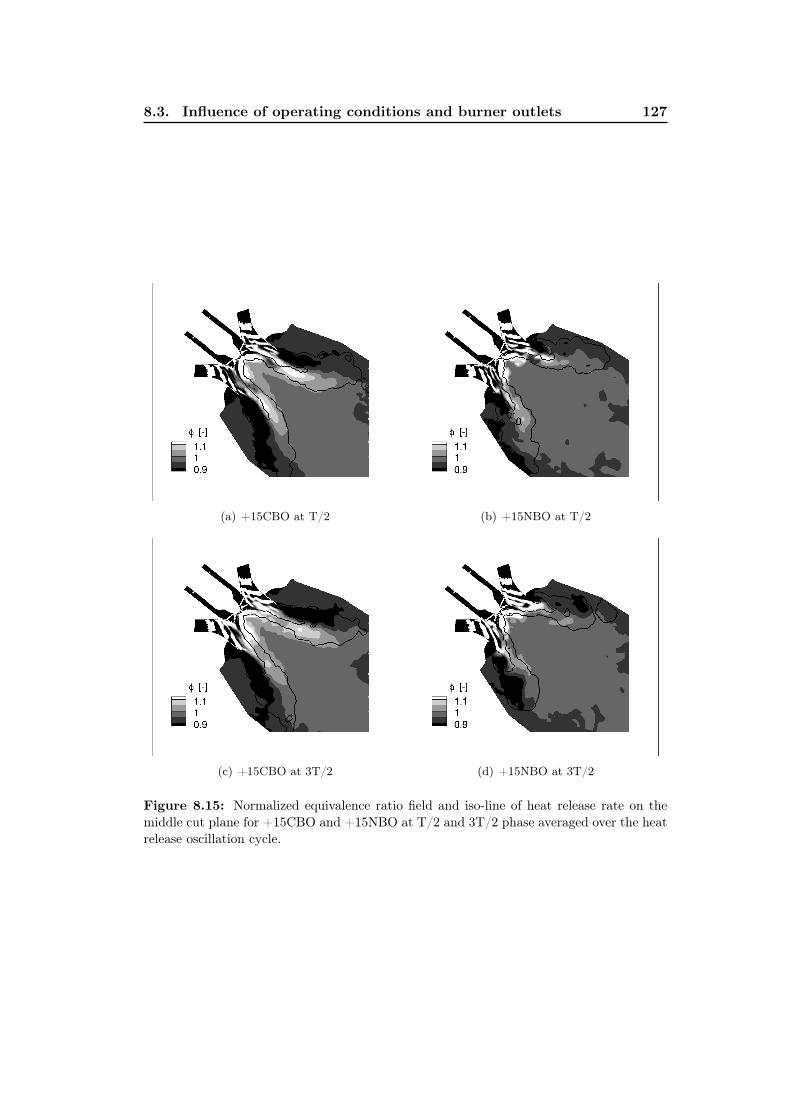
8.3. Influence of operating conditions and burner outlets 127
(a) +15CBO at T/2 (b) +15NBO at T/2
(c) +15CBO at 3T/2 (d) +15NBO at 3T/2
Figure 8.15: Normalized equivalence ratio field and iso-line of heat release rate on themiddle cut plane for +15CBO and +15NBO at T/2 and 3T/2 phase averaged over the heatrelease oscillation cycle.

128 Chapter 8. Acoustically perturbed flame
RMS temperature profiles reveal that the NBO cases undergo slightly stronger fluc-tuations than the CBO cases. Distinct equivalence ratio fields of the oscillation cyclereveal that mixture perturbations propagate similarly to and on the flame surfacefor both configurations.
The global flame response in terms of n and tau shows that the CBO cases have aslightly shorter time lag than the NBO cases although the flame is slightly longer.This result is contradictory to Krebs et al. [103] who states that the time lag in-creases when adding a CBO compared to the case with no CBO. Although anuncertainty exists regarding the values of amplitude and time delay found in thiswork, the shorter CBO delay is explained as follows: first, the length of the averagedflame is only slightly shorter in the NBO case as found in chapter 7. Second, eventhough hypothetically the time delay values could be shifted by 2π, a significantlyhigher time delay for the NBO case is less probable. To support this, the lengthof the flame is additionally evaluated defined as the distance from the lance to theflame tip. It is found that the CBO flame is about 1.15 times longer. The acousticfluctuation perturbs the flame front which is convectively transported to the flametip and the time needed even for a convective perturbation to reach this additionalpart is only of 1/5T based on the bulk velocity. This means that a different mech-anism is at play causing the NBO flame to react slightly later. The mean velocityprofiles in Fig. 7.10 to 7.14 show that the CBO cases possess a higher axial velocityat the burner outlet. Vortices are formed due to shear at the burner outlet in theouter flame region and in the inner region where the mass flow of axial and diagonalmeet. These vortices convect along the flame front and control the dynamic flameresponse. Since the convective velocity is higher in the CBO cases this can lead toa lower time delay as the differences in flame length are small. Sensiau et al. [158]noticed that even small changes in time delay can lead to important effects on thestability and found the transition between amplification and damping to be at halfthe period T with damping occurring at τ < T/2. The time lags found for thisfrequency f4 correspond to this. One can state furthermore, that a simple modeltaking only into account the flight time is not appropriate [51]: as shown by [150],even though FTF delay scales to first-order like the flame length divided by the bulkvelocity for very simple flames, additional mechanisms in real chambers make flighttime estimates of the delay doubtful in complex combustors. The amplitude of theglobal FTF varies only slightly for all cases. Local FTFs of all cases revealed that+15NBO and -15NBO behave similarly in terms of n and tau whereas differencesbetween +15CBO and -15CBO occur slightly for the amplitude in the inner flameregion and especially for the time delay.
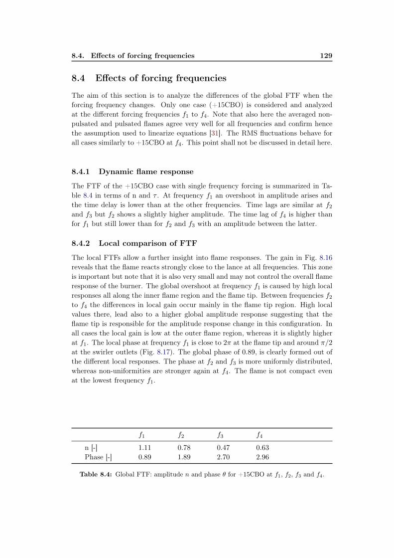
8.4. Effects of forcing frequencies 129
8.4 Effects of forcing frequencies
The aim of this section is to analyze the differences of the global FTF when theforcing frequency changes. Only one case (+15CBO) is considered and analyzedat the different forcing frequencies f1 to f4. Note that also here the averaged non-pulsated and pulsated flames agree very well for all frequencies and confirm hencethe assumption used to linearize equations [31]. The RMS fluctuations behave forall cases similarly to +15CBO at f4. This point shall not be discussed in detail here.
8.4.1 Dynamic flame response
The FTF of the +15CBO case with single frequency forcing is summarized in Ta-ble 8.4 in terms of n and τ . At frequency f1 an overshoot in amplitude arises andthe time delay is lower than at the other frequencies. Time lags are similar at f2
and f3 but f2 shows a slightly higher amplitude. The time lag of f4 is higher thanfor f1 but still lower than for f2 and f3 with an amplitude between the latter.
8.4.2 Local comparison of FTF
The local FTFs allow a further insight into flame responses. The gain in Fig. 8.16reveals that the flame reacts strongly close to the lance at all frequencies. This zoneis important but note that it is also very small and may not control the overall flameresponse of the burner. The global overshoot at frequency f1 is caused by high localresponses all along the inner flame region and the flame tip. Between frequencies f2
to f4 the differences in local gain occur mainly in the flame tip region. High localvalues there, lead also to a higher global amplitude response suggesting that theflame tip is responsible for the amplitude response change in this configuration. Inall cases the local gain is low at the outer flame region, whereas it is slightly higherat f1. The local phase at frequency f1 is close to 2π at the flame tip and around π/2at the swirler outlets (Fig. 8.17). The global phase of 0.89, is clearly formed out ofthe different local responses. The phase at f2 and f3 is more uniformly distributed,whereas non-uniformities are stronger again at f4. The flame is not compact evenat the lowest frequency f1.
f1 f2 f3 f4
n [-] 1.11 0.78 0.47 0.63
Phase [-] 0.89 1.89 2.70 2.96
Table 8.4: Global FTF: amplitude n and phase θ for +15CBO at f1, f2, f3 and f4.
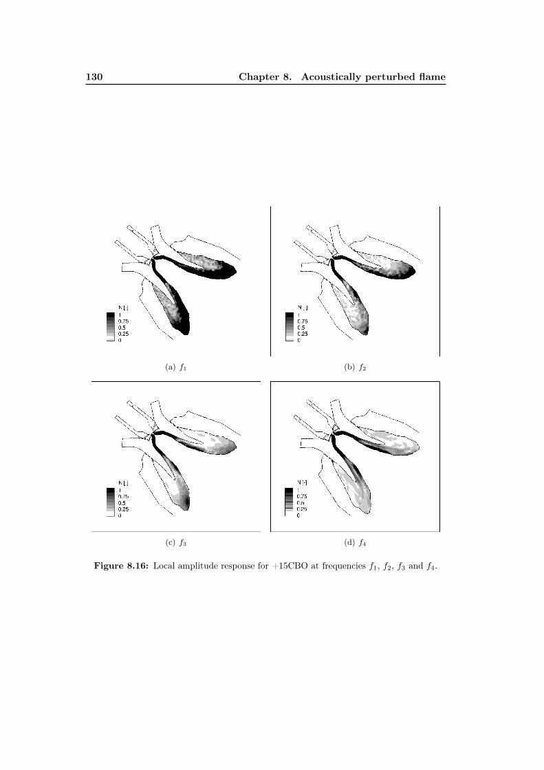
130 Chapter 8. Acoustically perturbed flame
(a) f1 (b) f2
(c) f3 (d) f4
Figure 8.16: Local amplitude response for +15CBO at frequencies f1, f2, f3 and f4.

8.4. Effects of forcing frequencies 131
(a) f1 (b) f2
(c) f3 (d) f4
Figure 8.17: Local phase response for +15CBO at frequencies f1, f2, f3 and f4.
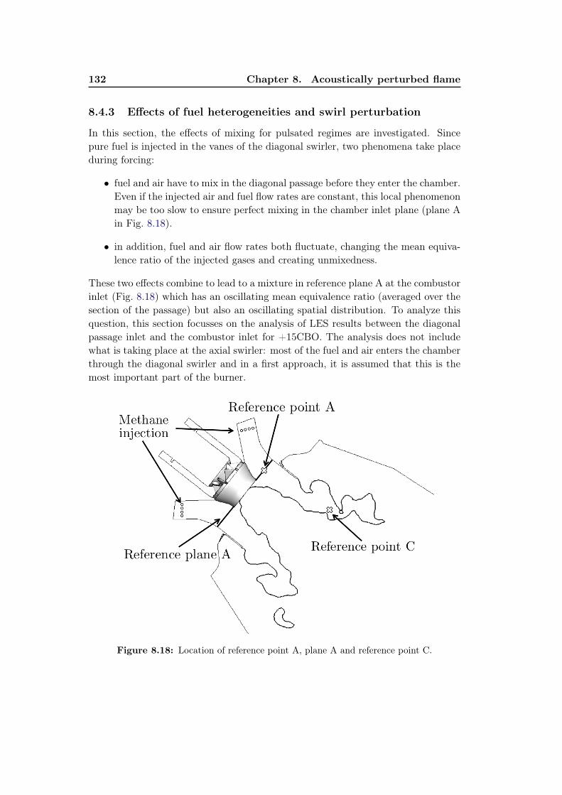
132 Chapter 8. Acoustically perturbed flame
8.4.3 Effects of fuel heterogeneities and swirl perturbation
In this section, the effects of mixing for pulsated regimes are investigated. Sincepure fuel is injected in the vanes of the diagonal swirler, two phenomena take placeduring forcing:
• fuel and air have to mix in the diagonal passage before they enter the chamber.Even if the injected air and fuel flow rates are constant, this local phenomenonmay be too slow to ensure perfect mixing in the chamber inlet plane (plane Ain Fig. 8.18).
• in addition, fuel and air flow rates both fluctuate, changing the mean equiva-lence ratio of the injected gases and creating unmixedness.
These two effects combine to lead to a mixture in reference plane A at the combustorinlet (Fig. 8.18) which has an oscillating mean equivalence ratio (averaged over thesection of the passage) but also an oscillating spatial distribution. To analyze thisquestion, this section focusses on the analysis of LES results between the diagonalpassage inlet and the combustor inlet for +15CBO. The analysis does not includewhat is taking place at the axial swirler: most of the fuel and air enters the chamberthrough the diagonal swirler and in a first approach, it is assumed that this is themost important part of the burner.
Figure 8.18: Location of reference point A, plane A and reference point C.

8.4. Effects of forcing frequencies 133
The global mixture fraction Z through the diagonal passage is calculated with:
Z =mCH4
mAir + mCH4(8.5)
and results from the fluctuating air mass flow rate at the diagonal inlet mAir
(Fig. 8.19) and the fuel mass flow rate through the premixing nozzle mCH4 (Fig. 8.20).Both flow rates are shown as normalized fluctuations m′/ ˙m over the forcing period.The velocity perturbation introduced at the inlet of the diagonal swirler leads to
0 1 2 3 4
−0.1
−0.05
0
0.05
0.1
t/T [−]
m’ a
ir/m
air [
−]
f1
f2
f3
f4
Figure 8.19: Relative variations of the air mass flow rate at diagonal inlet at frequenciesf1, f2, f3 and f4.
0 1 2 3 4−0.04
−0.02
0
0.02
0.04
t/T [−]
m’ fu
el/m
fuel [
−]
f1
f2
f3
f4
Figure 8.20: Relative variations of the fuel mass flow rate at diagonal inlet at frequenciesf1, f2, f3 and f4.
a perturbation of the air mass flow rate of the order of 5 to 10%. The fuel fluctua-tions result from the oscillating pressure perturbations at the injection holes: theydepend on the stiffness of the boundary condition imposed at the fuel inlet. Here,they lead to a relative modification of the fuel flow rate which is much less thanfor the air. Typically, the fuel flow rate varies by 1 to 2 % at most (Fig. 8.20)and a phase difference is visible. Since the air mass flow rate is fluctuating atmuch higher amplitude, this has only small effects on the global mixture fluctuation(Fig. 8.21) which fluctuates by 8 to 10 %. Fluctuations of mixture propagate at the

134 Chapter 8. Acoustically perturbed flame
convective speed to the flame front and are damped through the swirler as shownby the time variation of the mixture fraction averaged over the reference plane A inFig. 8.22. First the mixing fluctuations introduced at the diagonal inlet (Fig. 8.21)do not disappear in the passage: at the combustor inlet section (reference plane Ain Fig. 8.18) Z still changes by ±5%, compared to + or - 8 to 10 % at the diagonalinlet. The diagonal passage is not long enough to damp fuel heterogeneities intro-duced by the fluctuations. Second, as expected, higher frequencies (f4) are dampedmore than low frequency fluctuations (f1).
0 1 2 3 4
−0.1
−0.05
0
0.05
0.1
t/T [−]
Z’/Z
[−
]
f1
f2
f3
f4
Figure 8.21: Global mixture fraction (Eq. 8.5) at diagonal inlet for frequencies f1, f2, f3and f4.
0 1 2 3 4−0.1
−0.05
0
0.05
0.1
t/T [−]
Z’/Z
[−
]
f1
f2
f3
f4
Figure 8.22: Global mixture fraction averaged over reference plane A for frequencies f1,f2, f3 and f4.
A phase difference appears for the different frequencies indicating a different phasebetween axial velocity perturbation and mixture fraction oscillation. Following Kimet al. [82] this has an impact on the amplitude response of the flame: When thetwo perturbations are out of phase richer mixtures enter the combustion chamberwith low velocity, and mixtures with lower equivalence ratio reach the flame frontwith high velocity. The flame sees nearly the same amount of fuel during a cycle

8.4. Effects of forcing frequencies 135
of oscillation. Therefore, the heat release rate does not vary significantly and a lowamplitude response results.
In a first step, to see the impact of mixture fraction fluctuations over the heatrelease oscillation cycle, phase averaged solutions are shown in Fig. 8.23 and 8.24 atT/2 and 3T/2 respectively. Although the global FTF response is different (table 8.4),significant similarities are found: for all frequencies, the normalized equivalence ra-tio is the highest at the maximum of the global heat release and a richer mixturereaches the highest flame surface (on the inner flame in axial direction) for all oscil-lation cycles. Note that phase averaged solutions are taken for 2T , T/2, T and 3T/2
whereas only T/2 and 3T/2 are shown here. At 3T/2, the phase corresponding tothe lowest global heat release, equivalence ratio fluctuations meeting the flame front
(a) f1 (b) f2
(c) f3 (d) f4
Figure 8.23: Normalized equivalence ratio field and iso-line of heat release rate on themiddle cut plane for +15CBO phase averaged at the maximum of the heat release oscillationcycle for frequencies f1, f2, f3 and f4.
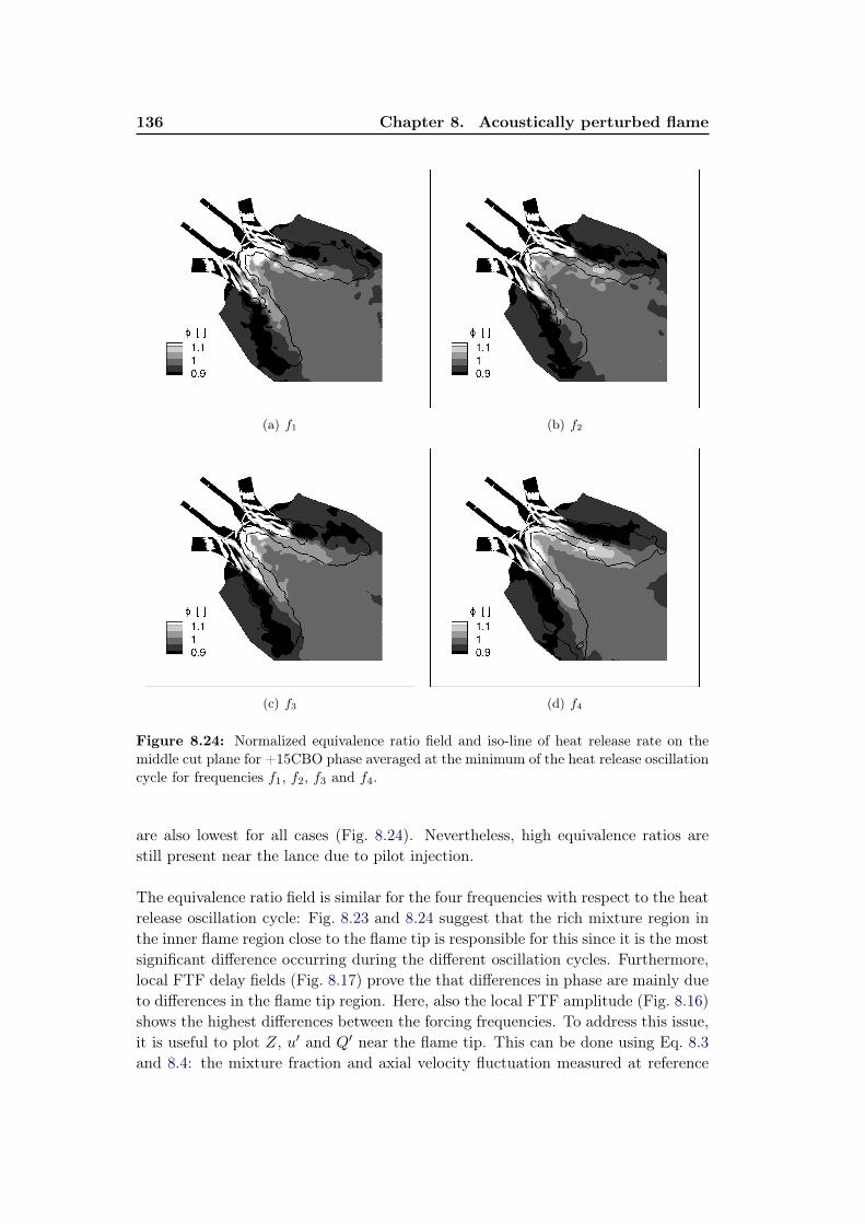
136 Chapter 8. Acoustically perturbed flame
(a) f1 (b) f2
(c) f3 (d) f4
Figure 8.24: Normalized equivalence ratio field and iso-line of heat release rate on themiddle cut plane for +15CBO phase averaged at the minimum of the heat release oscillationcycle for frequencies f1, f2, f3 and f4.
are also lowest for all cases (Fig. 8.24). Nevertheless, high equivalence ratios arestill present near the lance due to pilot injection.
The equivalence ratio field is similar for the four frequencies with respect to the heatrelease oscillation cycle: Fig. 8.23 and 8.24 suggest that the rich mixture region inthe inner flame region close to the flame tip is responsible for this since it is the mostsignificant difference occurring during the different oscillation cycles. Furthermore,local FTF delay fields (Fig. 8.17) prove the that differences in phase are mainly dueto differences in the flame tip region. Here, also the local FTF amplitude (Fig. 8.16)shows the highest differences between the forcing frequencies. To address this issue,it is useful to plot Z, u′ and Q′ near the flame tip. This can be done using Eq. 8.3and 8.4: the mixture fraction and axial velocity fluctuation measured at reference

8.4. Effects of forcing frequencies 137
plane A is shifted to a reference point C shown in Fig. 8.18. The mixture fractionfluctuation is transported with the convective velocity for which the bulk velocityis taken. The axial velocity fluctuation propagates with the speed of sound whichis given through the inlet temperature. For simplicity reasons, damping effects onthe fluctuations are not accounted for. The resulting relative axial velocity, mixturefraction and heat release fluctuation at reference point C are shown in Fig. 8.25to 8.28 for frequencies f1 to f4 leading to an interesting observation (Table 8.5). Atpoint C, the phase between mixture fraction Z ′ and heat release Q′ fluctuation isthe same for all frequencies while the phase between velocity perturbation u′ andQ′ changes significantly (it increases with frequency). This result suggests that theheat release is synchronized with the fluctuation of mixing and not with the velocityfor this regime.
1 2 3 4
−0.1
−0.05
0
0.05
0.1
t/T [−]
uax
′/uax
Z′/Z
Q′/Q
Figure 8.25: Relative axial velocity, mixture fraction and heat release fluctuation atreference point C for frequency f1.
1 2 3 4
−0.1
−0.05
0
0.05
0.1
t/T [−]
uax
′/uax
Z′/Z
Q′/Q
Figure 8.26: Relative axial velocity, mixture fraction and heat release fluctuation atreference point C for frequency f2.
A third effect of the ingoing acoustic wave besides the acoustic perturbation normalto the flame front and the convectively transported mixture fluctuation is the effectof swirl number perturbations [59, 84, 173]. When acoustic perturbations impingethe swirler, an axial and azimuthal velocity fluctuation is created travelling with

138 Chapter 8. Acoustically perturbed flame
1 2 3 4
−0.1
−0.05
0
0.05
0.1
t/T [−]
uax
′/uax
Z′/Z
Q′/Q
Figure 8.27: Relative axial velocity, mixture fraction and heat release fluctuation atreference point C for frequency f3.
1 2 3 4
−0.1
−0.05
0
0.05
0.1
t/T [−]
uax
′/uax
Z′/Z
Q′/Q
Figure 8.28: Relative axial velocity, mixture fraction and heat release fluctuation atreference point C for frequency f4.
f1 f2 f3 f4
Phase between Z ′ and Q′ [-] 1.69 1.64 1.52 1.26
Phase between u′ and Q′ [-] 0.27 0.77 2.21 2.91
Table 8.5: Phase angle (radian) of mixture fraction and axial velocity to the heat releaserate oscillation at reference point C for f1, f2, f3 and f4.
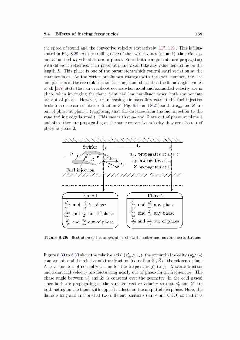
8.4. Effects of forcing frequencies 139
the speed of sound and the convective velocity respectively [117, 119]. This is illus-trated in Fig. 8.29. At the trailing edge of the swirler vanes (plane 1), the axial uaxand azimuthal uθ velocities are in phase. Since both components are propagatingwith different velocities, their phase at plane 2 can take any value depending on thelength L. This phase is one of the parameters which control swirl variation at thechamber inlet. As the vortex breakdown changes with the swirl number, the sizeand position of the recirculation zones change and affect thus the flame angle. Palieset al. [117] state that an overshoot occurs when axial and azimuthal velocity are inphase when impinging the flame front and low amplitude when both componentsare out of phase. However, an increasing air mass flow rate at the fuel injectionleads to a decrease of mixture fraction Z (Fig. 8.19 and 8.21) so that uax and Z areout of phase at plane 1 (supposing that the distance from the fuel injection to thevane trailing edge is small). This means that uθ and Z are out of phase at plane 1and since they are propagating at the same convective velocity they are also out ofphase at plane 2.
Figure 8.29: Illustration of the propagation of swirl number and mixture perturbations.
Figure 8.30 to 8.33 show the relative axial (u′ax/uax), the azimuthal velocity (u′θ/uθ)components and the relative mixture fraction fluctuation Z ′/Z at the reference planeA as a function of normalized time for the frequencies f1 to f4. Mixture fractionand azimuthal velocity are fluctuating nearly out of phase for all frequencies. Thephase angle between u′θ and Z ′ is constant over the geometry (in the cold gases)since both are propagating at the same convective velocity so that u′θ and Z ′ areboth acting on the flame with opposite effects on the amplitude response. Here, theflame is long and anchored at two different positions (lance and CBO) so that it is

140 Chapter 8. Acoustically perturbed flame
not clear where both components act most importantly on the flame.
1 2 3 4
−0.1
−0.05
0
0.05
0.1
t/T [−]
uax
′/uax
uθ′/u
θ
Z′/Z
Figure 8.30: Relative fluctuation of axial velocity u′ax/ ¯uax, azimuthal velocity u′θ/uθ andmixture fraction Z ′/Z at reference plane A for frequency f1.
1 2 3 4
−0.1
−0.05
0
0.05
0.1
t/T [−]
uax
′/uax
uθ′/u
θ
Z′/Z
Figure 8.31: Relative fluctuation of axial velocity u′ax/ ¯uax, azimuthal velocity u′θ/uθ andmixture fraction Z ′/Z at reference plane A for frequency f2.
8.4.4 Concluding remarks
The dynamic flame response for one case (+15CBO) at four frequencies showed dif-ferences in the global FTF for the amplitude as well as the time delay. The localFTF gain fields reveal that these differences are due to different responses at theflame tip and along the inner flame region. The flame is not compact as evidenced bythe local FTF delay fields. Phase averaged solutions over the heat release oscillationcycle show strong similarities between the equivalence ratio field at the different fre-quencies. Rich mixture enters the region close to the flame tip in all cases. Mixturefraction perturbation at the tip have a similar phase to the heat release oscillationfor the four frequencies suggesting that the mixture fraction fluctuation at leastpartially controls the FTF delay. Since the mixture fraction propagates at the con-vective speed, the changes in global time delay can be explained. Although this isthe important mechanism in this configuration, the effect of axial velocity on the

8.4. Effects of forcing frequencies 141
1 2 3 4
−0.1
−0.05
0
0.05
0.1
t/T [−]
uax
′/uax
uθ′/u
θ
Z′/Z
Figure 8.32: Relative fluctuation of axial velocity u′ax/ ¯uax, azimuthal velocity u′θ/uθ andmixture fraction Z ′/Z at reference plane A for frequency f3.
1 2 3 4
−0.1
−0.05
0
0.05
0.1
t/T [−]
uax
′/uax
uθ′/u
θ
Z′/Z
Figure 8.33: Relative fluctuation of axial velocity u′ax/ ¯uax, azimuthal velocity u′θ/uθ andmixture fraction Z ′/Z at reference plane A for frequency f4.
global FTF is still present. Furthermore, azimuthal velocity fluctuations are prop-agating out of phase with the mixture fraction oscillations. Its impact (and also ofthe mixture fraction oscillation) on the global FTF gain still remains a matter ofinvestigation.
Obviously, the present analysis fails to clearly identify individual mechanisms con-trolling FTFs because they all play a role at the same time. In the next chapter, anew strategy will be utilized: additional LES are performed to isolate mechanismsand study their effects separately. In a first simulation a fully premixed flow is in-jected in the diagonal passage in order to investigate only the effect of axial velocityperturbation. Then, only fuel is pulsated at the diagonal inlet to analyze only theeffect of mixture fraction fluctuation decoupled from the axial velocity perturbation.

Chapter 9
Identification of mechanismscontrolling FTFs
Contents9.1 Effects of mass flow rate perturbation . . . . . . . . . . . . . 145
9.1.1 Mean reacting flow fields . . . . . . . . . . . . . . . . . . . . 1459.1.2 Dynamics of the reacting flow fields . . . . . . . . . . . . . . 1499.1.3 Concluding remarks . . . . . . . . . . . . . . . . . . . . . . . 150
9.2 Effects of mixture fluctuation . . . . . . . . . . . . . . . . . . 1529.2.1 Dynamic flame response . . . . . . . . . . . . . . . . . . . . . 1539.2.2 Propagation of mixing heterogeneities . . . . . . . . . . . . . 1549.2.3 Swirl number perturbation . . . . . . . . . . . . . . . . . . . 1609.2.4 Concluding remarks . . . . . . . . . . . . . . . . . . . . . . . 160
9.3 Combined Flame Transfer Function approach . . . . . . . . 161
The mechanisms controlling FTF have been studied extensively for simple labo-ratory flames but much less information is available for real gas turbines. Previouschapters have shown that one of the specificities of gas turbine chambers is that sev-eral mechanisms control the flame dynamics (Fig. 9.1). The fluctuating air and fuelinlet mass flow rates in the diagonal swirler cause oscillations of mixture fraction,axial velocity and swirl number which combine and act on the flame. When LES ofFTF are performed, they integrate these three mechanisms and the LES results arecertainly valid. However, understanding what controls FTF and how they can bemodified requires to be able to isolate mechanisms. Additional LES are performedhere to reach this goal.
This chapters’ goal is to exclude one mechanism after the other to study separatelyits effect on this complex flame. Therefore the +15CBO case will be considered atone frequency f4 and compared against two additional LES of the same geometry:
• For the first one, a fully premixed flow is passing through the diagonal swirler(Section 9.1) thereby cancelling any potential effect on the FTF due to mod-ulated mixing and focussing on the effect of mass flow rate perturbation.
• A second simulation is performed in Section 9.2 where only the fuel at thediagonal swirler is fluctuated and the main air mass flow rate through the
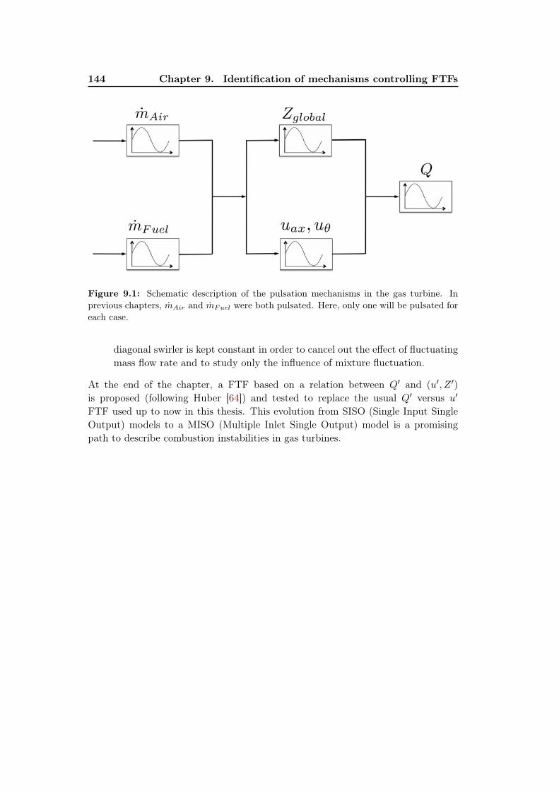
144 Chapter 9. Identification of mechanisms controlling FTFs
Figure 9.1: Schematic description of the pulsation mechanisms in the gas turbine. Inprevious chapters, mAir and mFuel were both pulsated. Here, only one will be pulsated foreach case.
diagonal swirler is kept constant in order to cancel out the effect of fluctuatingmass flow rate and to study only the influence of mixture fluctuation.
At the end of the chapter, a FTF based on a relation between Q′ and (u′, Z ′)is proposed (following Huber [64]) and tested to replace the usual Q′ versus u′
FTF used up to now in this thesis. This evolution from SISO (Single Input SingleOutput) models to a MISO (Multiple Inlet Single Output) model is a promisingpath to describe combustion instabilities in gas turbines.
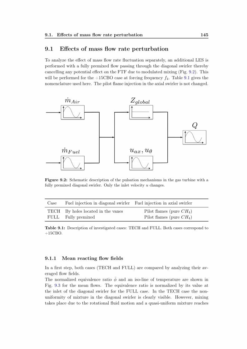
9.1. Effects of mass flow rate perturbation 145
9.1 Effects of mass flow rate perturbation
To analyze the effect of mass flow rate fluctuation separately, an additional LES isperformed with a fully premixed flow passing through the diagonal swirler therebycancelling any potential effect on the FTF due to modulated mixing (Fig. 9.2). Thiswill be performed for the +15CBO case at forcing frequency f4. Table 9.1 gives thenomenclature used here. The pilot flame injection in the axial swirler is not changed.
Figure 9.2: Schematic description of the pulsation mechanisms in the gas turbine with afully premixed diagonal swirler. Only the inlet velocity u changes.
Case Fuel injection in diagonal swirler Fuel injection in axial swirler
TECH By holes located in the vanes Pilot flames (pure CH4)FULL Fully premixed Pilot flames (pure CH4)
Table 9.1: Description of investigated cases: TECH and FULL. Both cases correspond to+15CBO.
9.1.1 Mean reacting flow fields
In a first step, both cases (TECH and FULL) are compared by analyzing their av-eraged flow fields.The normalized equivalence ratio φ and an iso-line of temperature are shown inFig. 9.3 for the mean flows. The equivalence ratio is normalized by its value atthe inlet of the diagonal swirler for the FULL case. In the TECH case the non-uniformity of mixture in the diagonal swirler is clearly visible. However, mixingtakes place due to the rotational fluid motion and a quasi-uniform mixture reaches

146 Chapter 9. Identification of mechanisms controlling FTFs
Figure 9.3: Normalized averaged equivalence ratio field and temperature iso-line for theTECH (left) and the FULL (right) case.
the flame front. Of course, for the FULL case, the mixture in the diagonal swirlerhas a constant equivalence ratio (φ = 1). Figure 9.3 shows that the two flames arevery similar in terms of shapes. The mean fields of both configurations are similarand remain similar with the forced fields (not shown): the assumption used to lin-earize equations [31] is fulfilled here too. For the sake of completeness, the flames ofthe technically premixed and fully premixed case are only shortly compared in termsof averaged pulsated solutions in Fig. 9.4 and 9.5 showing profiles in terms of meanand RMS temperature respectively. Very good agreement is found for both flamesfor the location and magnitude of extrema in all flame regions. RMS temperatureprofiles also agree well for both flames.
Mixing can be analyzed by plotting the probability density functions (PDF) ofnormalized heat release versus local equivalence ratio φ (Fig. 9.6). While the overallheat release is constant for both cases, a different heat release distribution over φis found. The TECH flame produces slightly less heat around φ = 1 and more atφ = 0.8 than the FULL case but differences between the two cases for the mean floware limited. The next step consists of analyzing the influence of these differences onthe forced flame.
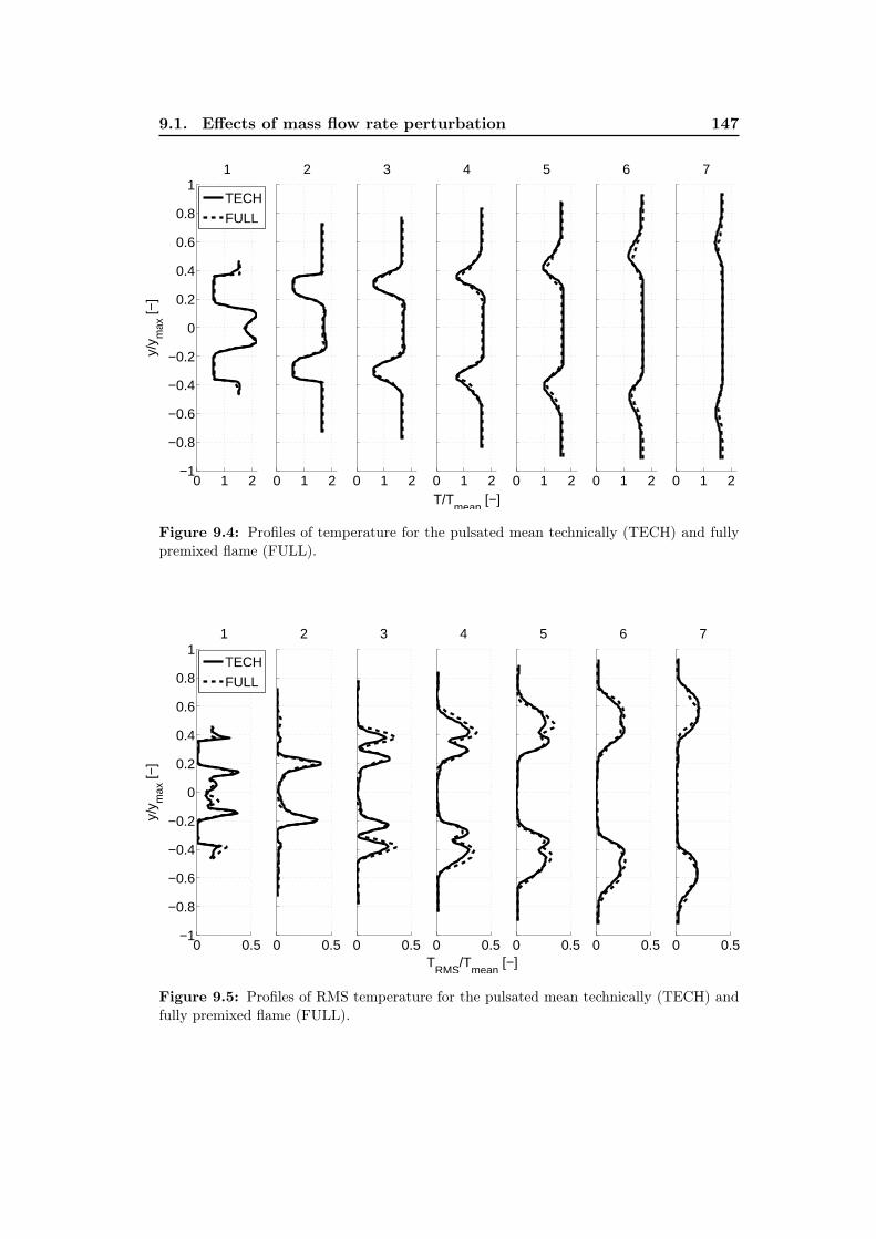
9.1. Effects of mass flow rate perturbation 147
0 1 2−1
−0.8
−0.6
−0.4
−0.2
0
0.2
0.4
0.6
0.8
1
y/y
ma
x [
−]
1
0 1 2
2
0 1 2
3
0 1 2
T/Tmean
[−]
4
0 1 2
5
0 1 2
6
0 1 2
7
TECH
FULL
Figure 9.4: Profiles of temperature for the pulsated mean technically (TECH) and fullypremixed flame (FULL).
0 0.5−1
−0.8
−0.6
−0.4
−0.2
0
0.2
0.4
0.6
0.8
1
y/y
ma
x [
−]
1
0 0.5
2
0 0.5
3
0 0.5
TRMS
/Tmean
[−]
4
0 0.5
5
0 0.5
6
0 0.5
7
TECH
FULL
Figure 9.5: Profiles of RMS temperature for the pulsated mean technically (TECH) andfully premixed flame (FULL).

148 Chapter 9. Identification of mechanisms controlling FTFs
(a) TECH
(b) FULL
Figure 9.6: PDF of the TECH and the FULL case for the averaged and the pulsatedaveraged flame (the equivalence ratio is normalized by its value in the diagonal passage).
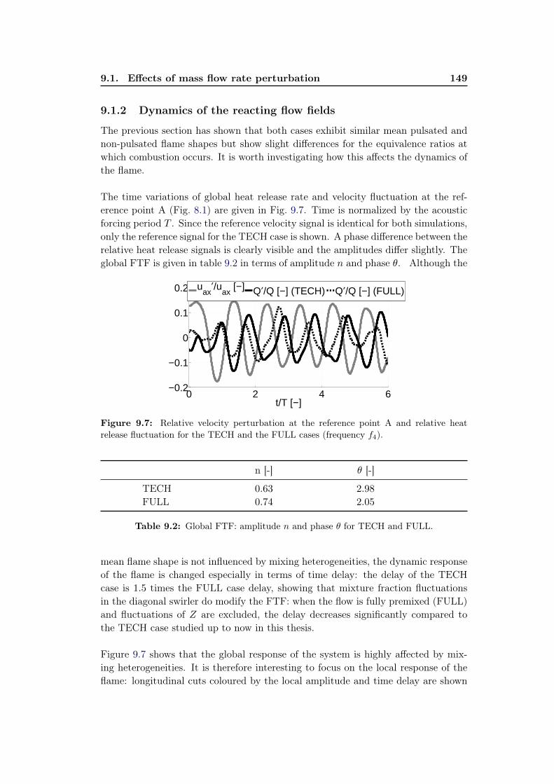
9.1. Effects of mass flow rate perturbation 149
9.1.2 Dynamics of the reacting flow fields
The previous section has shown that both cases exhibit similar mean pulsated andnon-pulsated flame shapes but show slight differences for the equivalence ratios atwhich combustion occurs. It is worth investigating how this affects the dynamics ofthe flame.
The time variations of global heat release rate and velocity fluctuation at the ref-erence point A (Fig. 8.1) are given in Fig. 9.7. Time is normalized by the acousticforcing period T . Since the reference velocity signal is identical for both simulations,only the reference signal for the TECH case is shown. A phase difference between therelative heat release signals is clearly visible and the amplitudes differ slightly. Theglobal FTF is given in table 9.2 in terms of amplitude n and phase θ. Although the
0 2 4 6−0.2
−0.1
0
0.1
0.2
t/T [−]
uax
′/uax
[−] Q′/Q [−] (TECH) Q′/Q [−] (FULL)
Figure 9.7: Relative velocity perturbation at the reference point A and relative heatrelease fluctuation for the TECH and the FULL cases (frequency f4).
n [-] θ [-]
TECH 0.63 2.98
FULL 0.74 2.05
Table 9.2: Global FTF: amplitude n and phase θ for TECH and FULL.
mean flame shape is not influenced by mixing heterogeneities, the dynamic responseof the flame is changed especially in terms of time delay: the delay of the TECHcase is 1.5 times the FULL case delay, showing that mixture fraction fluctuationsin the diagonal swirler do modify the FTF: when the flow is fully premixed (FULL)and fluctuations of Z are excluded, the delay decreases significantly compared tothe TECH case studied up to now in this thesis.
Figure 9.7 shows that the global response of the system is highly affected by mix-ing heterogeneities. It is therefore interesting to focus on the local response of theflame: longitudinal cuts coloured by the local amplitude and time delay are shown

150 Chapter 9. Identification of mechanisms controlling FTFs
in Fig. 9.8 and Fig. 9.9 respectively. The amplitude response of the TECH case isintense near the lance and in the inner flame region. At the flame tip the amplitudevaries strongly and is non-uniform with higher values on the inner side and lower atthe outer flame. The FULL case shows less intense amplitude near the lance thanthe TECH case but behaves similarly in the inner flame region where a shear layerseparates the flows of the axial and diagonal swirlers. Close to the flame tip and inthe outer flame region, the amplitude is almost uniformly distributed but at slightlylower values than the TECH case. Although the global amplitude of both cases issimilar, the local FTF fields reveal significant differences. The mixture fluctuationsin the TECH case are phased with the velocity perturbations and propagate alongthe flame front affecting the local amplitude of the flame to higher and lower valueswhereas the FULL case shows a more uniformly distributed amplitude along theflame. The phase (Fig. 9.9) is in the FULL case similar to TECH in the vicinity ofthe lance. Differences are found at the flame tip underlying the importance of theflame tip reaction on the global time delay. In TECH, the reaction of the flame tipis predominantly determined by its phase to the mixture fraction fluctuation closeto it (section 8.4).
9.1.3 Concluding remarks
LES reveals that both cases, the fully premixed (FULL) and the technically pre-mixed (TECH), exhibit similar mean pulsated and non-pulsated flame shapes butPDFs show slight differences for the equivalence ratio distribution participating inheat release production. Mixture perturbations have an important effect on theglobal FTFs: the FTF delay for the TECH case is 1.5 times larger than for theFULL case and the interactive index slightly lower. Local FTF fields show thatmixture heterogeneities propagating in the diagonal swirler lead to locally differ-ent responses over the flame region, whereas the FULL flame shows similar valuesof amplitude and time delay over the whole flame. The following section gives adeeper investigation on the effect of mixture heterogeneities while only forcing thefuel in the diagonal swirler and hence excluding the effect of air mass flow rateperturbations.
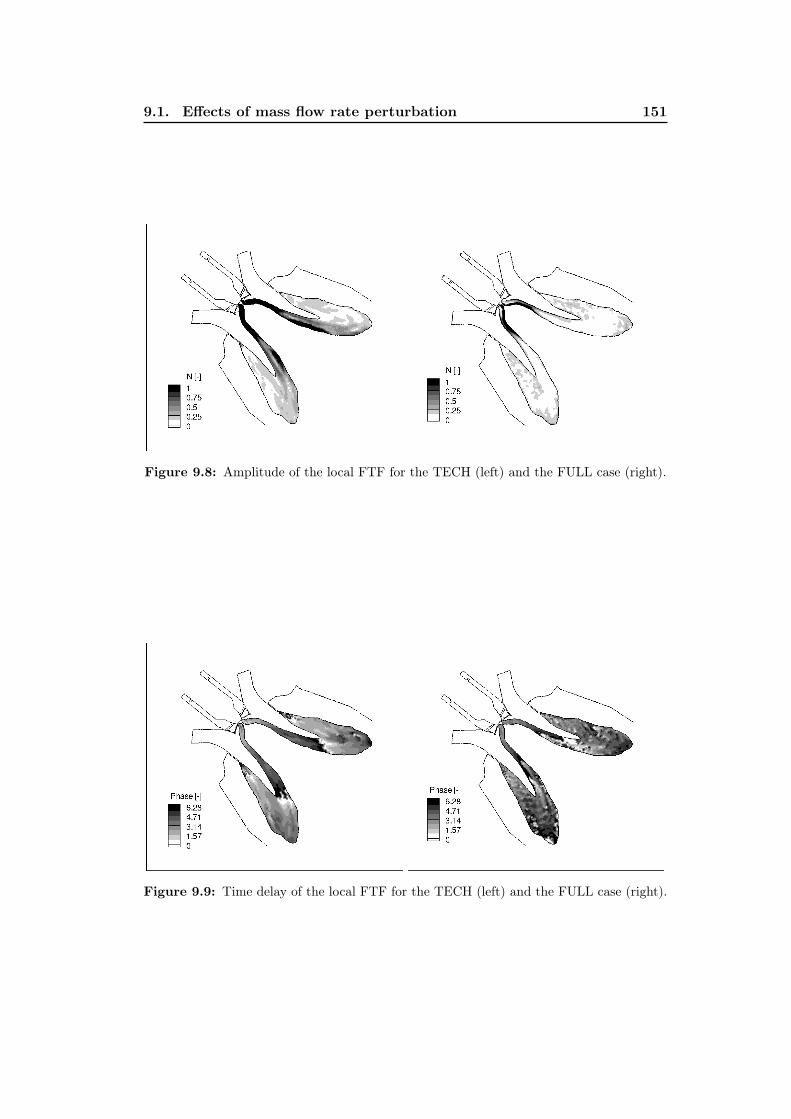
9.1. Effects of mass flow rate perturbation 151
Figure 9.8: Amplitude of the local FTF for the TECH (left) and the FULL case (right).
Figure 9.9: Time delay of the local FTF for the TECH (left) and the FULL case (right).
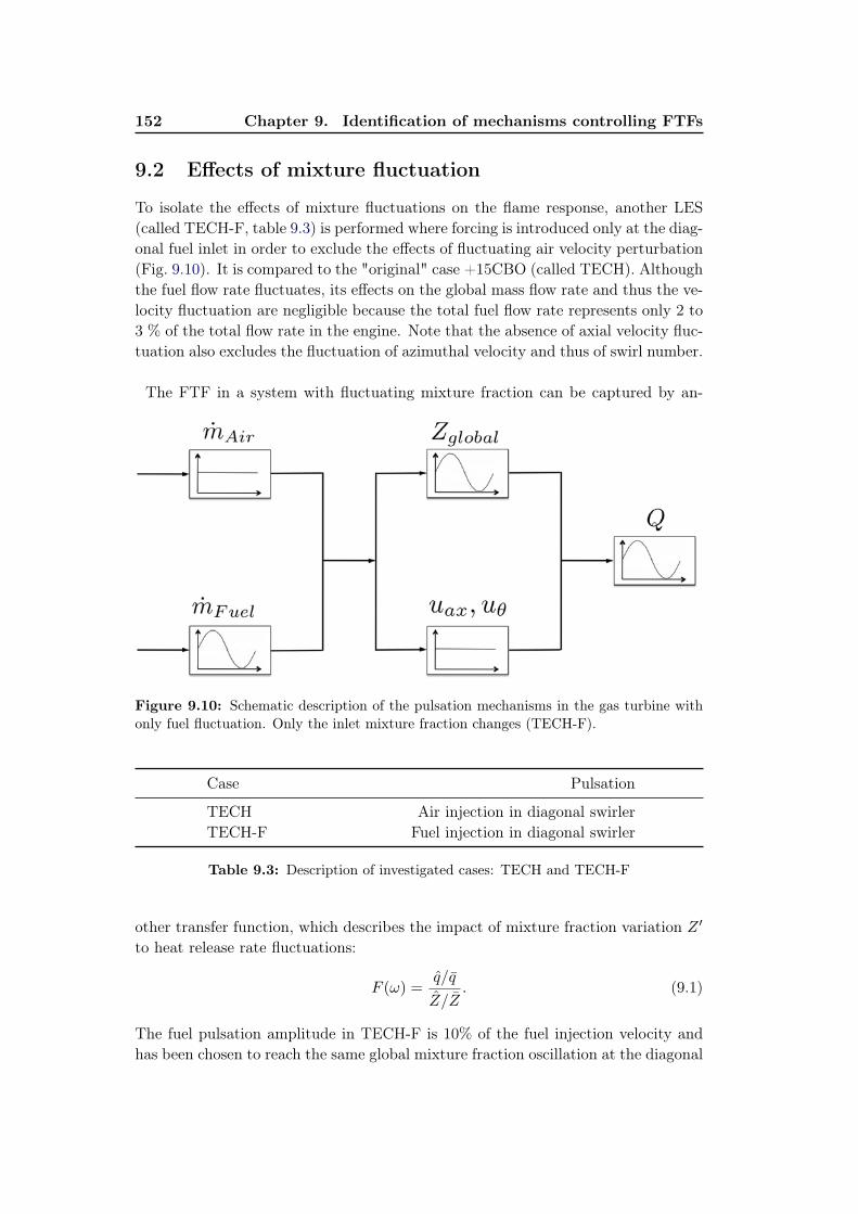
152 Chapter 9. Identification of mechanisms controlling FTFs
9.2 Effects of mixture fluctuation
To isolate the effects of mixture fluctuations on the flame response, another LES(called TECH-F, table 9.3) is performed where forcing is introduced only at the diag-onal fuel inlet in order to exclude the effects of fluctuating air velocity perturbation(Fig. 9.10). It is compared to the "original" case +15CBO (called TECH). Althoughthe fuel flow rate fluctuates, its effects on the global mass flow rate and thus the ve-locity fluctuation are negligible because the total fuel flow rate represents only 2 to3 % of the total flow rate in the engine. Note that the absence of axial velocity fluc-tuation also excludes the fluctuation of azimuthal velocity and thus of swirl number.
The FTF in a system with fluctuating mixture fraction can be captured by an-
Figure 9.10: Schematic description of the pulsation mechanisms in the gas turbine withonly fuel fluctuation. Only the inlet mixture fraction changes (TECH-F).
Case Pulsation
TECH Air injection in diagonal swirlerTECH-F Fuel injection in diagonal swirler
Table 9.3: Description of investigated cases: TECH and TECH-F
other transfer function, which describes the impact of mixture fraction variation Z ′
to heat release rate fluctuations:
F (ω) =q/q
Z/Z. (9.1)
The fuel pulsation amplitude in TECH-F is 10% of the fuel injection velocity andhas been chosen to reach the same global mixture fraction oscillation at the diagonal
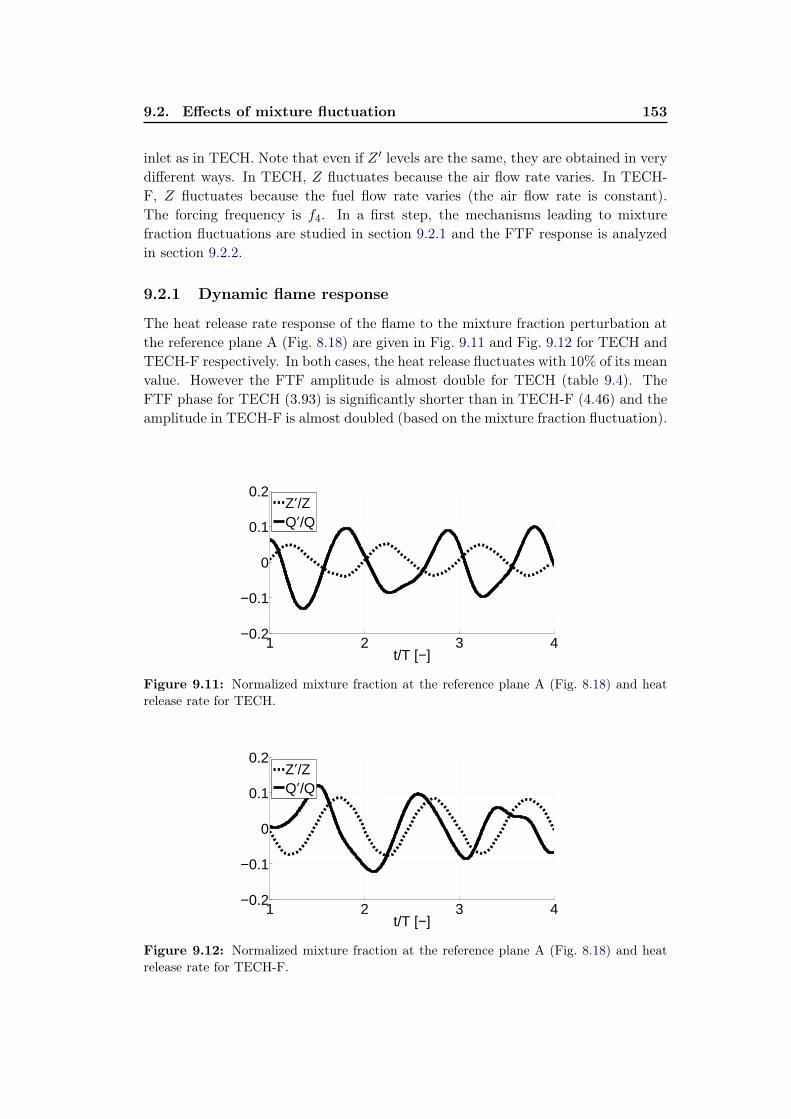
9.2. Effects of mixture fluctuation 153
inlet as in TECH. Note that even if Z ′ levels are the same, they are obtained in verydifferent ways. In TECH, Z fluctuates because the air flow rate varies. In TECH-F, Z fluctuates because the fuel flow rate varies (the air flow rate is constant).The forcing frequency is f4. In a first step, the mechanisms leading to mixturefraction fluctuations are studied in section 9.2.1 and the FTF response is analyzedin section 9.2.2.
9.2.1 Dynamic flame response
The heat release rate response of the flame to the mixture fraction perturbation atthe reference plane A (Fig. 8.18) are given in Fig. 9.11 and Fig. 9.12 for TECH andTECH-F respectively. In both cases, the heat release fluctuates with 10% of its meanvalue. However the FTF amplitude is almost double for TECH (table 9.4). TheFTF phase for TECH (3.93) is significantly shorter than in TECH-F (4.46) and theamplitude in TECH-F is almost doubled (based on the mixture fraction fluctuation).
1 2 3 4−0.2
−0.1
0
0.1
0.2
t/T [−]
Z′/Z
Q′/Q
Figure 9.11: Normalized mixture fraction at the reference plane A (Fig. 8.18) and heatrelease rate for TECH.
1 2 3 4−0.2
−0.1
0
0.1
0.2
t/T [−]
Z′/Z
Q′/Q
Figure 9.12: Normalized mixture fraction at the reference plane A (Fig. 8.18) and heatrelease rate for TECH-F.
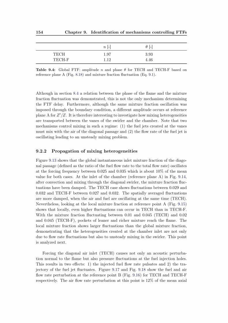
154 Chapter 9. Identification of mechanisms controlling FTFs
n [-] θ [-]
TECH 1.97 3.93
TECH-F 1.12 4.46
Table 9.4: Global FTF: amplitude n and phase θ for TECH and TECH-F based onreference plane A (Fig. 8.18) and mixture fraction fluctuation (Eq. 9.1).
Although in section 8.4 a relation between the phase of the flame and the mixturefraction fluctuation was demonstrated, this is not the only mechanism determiningthe FTF delay. Furthermore, although the same mixture fraction oscillation wasimposed through the boundary condition, a different amplitude occurs at referenceplane A for Z ′/Z. It is therefore interesting to investigate how mixing heterogeneitiesare transported between the vanes of the swirler and the chamber. Note that twomechanisms control mixing in such a regime: (1) the fuel jets created at the vanesmust mix with the air of the diagonal passage and (2) the flow rate of the fuel jet isoscillating leading to an unsteady mixing problem.
9.2.2 Propagation of mixing heterogeneities
Figure 9.13 shows that the global instantaneous inlet mixture fraction of the diago-nal passage (defined as the ratio of the fuel flow rate to the total flow rate) oscillatesat the forcing frequency between 0.025 and 0.035 which is about 10% of the meanvalue for both cases. At the inlet of the chamber (reference plane A) in Fig. 9.14,after convection and mixing through the diagonal swirler, the mixture fraction fluc-tuations have been damped. The TECH case shows fluctuations between 0.029 and0.032 and TECH-F between 0.027 and 0.032. The spatially averaged fluctuationsare more damped, when the air and fuel are oscillating at the same time (TECH).Nevertheless, looking at the local mixture fraction at reference point A (Fig. 9.15)shows that locally, even higher fluctuations can occur in TECH than in TECH-F.With the mixture fraction fluctuating between 0.01 and 0.045 (TECH) and 0.02
and 0.045 (TECH-F), pockets of leaner and richer mixture reach the flame. Thelocal mixture fraction shows larger fluctuations than the global mixture fraction,demonstrating that the heterogeneities created at the chamber inlet are not onlydue to flow rate fluctuations but also to unsteady mixing in the swirler. This pointis analyzed next.
Forcing the diagonal air inlet (TECH) causes not only an acoustic perturba-tion normal to the flame but also pressure fluctuations at the fuel injection holes.This results in two effects: 1) the injected fuel flow rate pulsates and 2) the tra-jectory of the fuel jet fluctuates. Figure 9.17 and Fig. 9.18 show the fuel and airflow rate perturbation at the reference point B (Fig. 9.16) for TECH and TECH-Frespectively. The air flow rate perturbation at this point is 12% of the mean axial
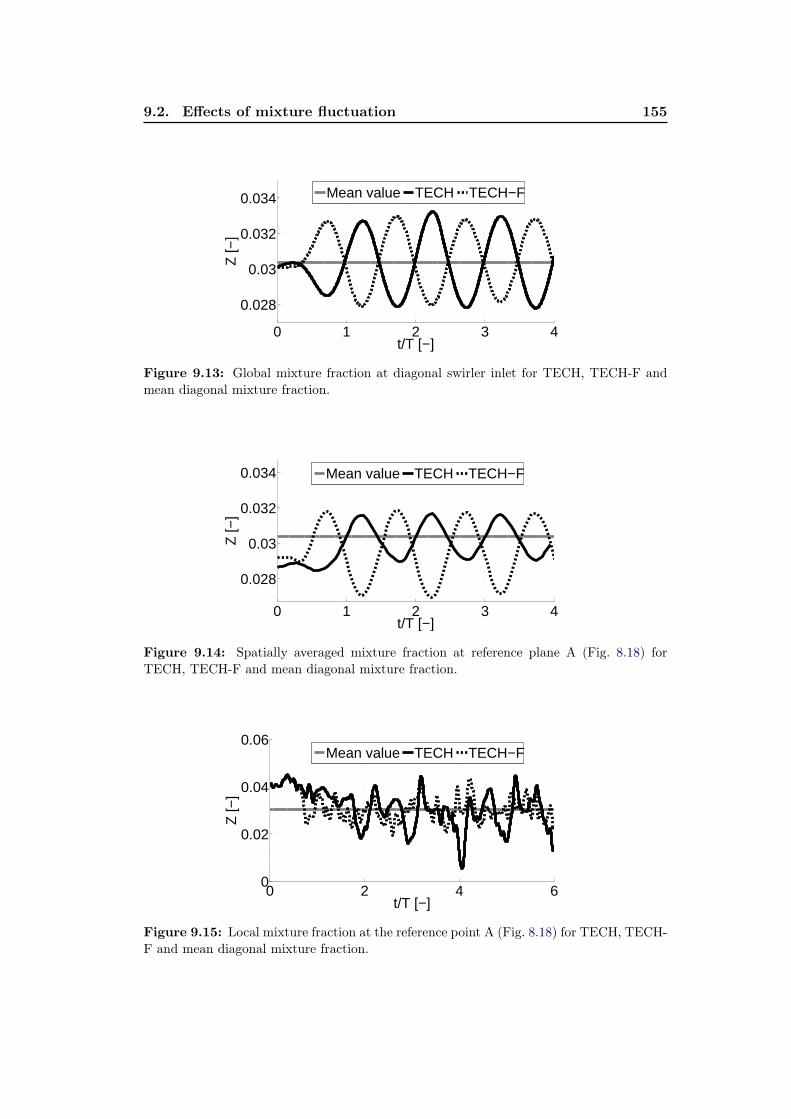
9.2. Effects of mixture fluctuation 155
0 1 2 3 4
0.028
0.03
0.032
0.034
Z [−
]
t/T [−]
Mean value TECH TECH−F
Figure 9.13: Global mixture fraction at diagonal swirler inlet for TECH, TECH-F andmean diagonal mixture fraction.
0 1 2 3 4
0.028
0.03
0.032
0.034
t/T [−]
Z [−
]
Mean value TECH TECH−F
Figure 9.14: Spatially averaged mixture fraction at reference plane A (Fig. 8.18) forTECH, TECH-F and mean diagonal mixture fraction.
0 2 4 60
0.02
0.04
0.06
Z [−
]
t/T [−]
Mean value TECH TECH−F
Figure 9.15: Local mixture fraction at the reference point A (Fig. 8.18) for TECH, TECH-F and mean diagonal mixture fraction.

156 Chapter 9. Identification of mechanisms controlling FTFs
Figure 9.16: Relative fuel and air velocity at reference point B.
component and the fuel flow rate fluctuation 5% in the TECH case whereas forTECH-F 7% of air and 10% of fuel flow rate perturbation are present. Comparedto TECH the fuel flow rate perturbation is higher and the air perturbation is lesspronounced. Note that the small fuel injection holes are fed by a plenum (Fig. 9.16)where the most important pressure drop occurs through the holes. This meansthat even when a non-reflecting boundary condition is imposed at the plenum, theimpedance and therefore the fluctuations of fuel flow rate are captured realisticallyin TECH by the LES set-up used here.
1 2 3 4
−0.1
−0.05
0
0.05
0.1
t/T [−]
vAir
[−]
vFuel
[−]
Figure 9.17: TECH: Relative fuel and air velocity perturbation at reference point B(Fig. 9.16).
The fuel velocity perturbation causes a variation of the fuel jet trajectory as wellas a perturbation in mixture illustrated by two snapshots from LES in Fig. 9.19showing an iso-surface of methane mass fraction, the normalized equivalence ratiofield and a temperature iso-surface (T/Tmean = 1.3) for TECH. The oscillations of

9.2. Effects of mixture fluctuation 157
1 2 3 4
−0.1
−0.05
0
0.05
0.1
t/T [−]
vAir
[−]
vFuel
[−]
Figure 9.18: TECH-F: Relative fuel and air velocity perturbation at reference point B(Fig. 9.16).
(a) Jet trajectory maximum (b) Jet trajectory minimum
(c) Jet trajectory maximum (zoom) (d) Jet trajectory minimum (zoom)
Figure 9.19: Jet trajectory visualized as YCH4 iso-surface and normalized equivalenceratio field for two distinct snapshots (TECH case).
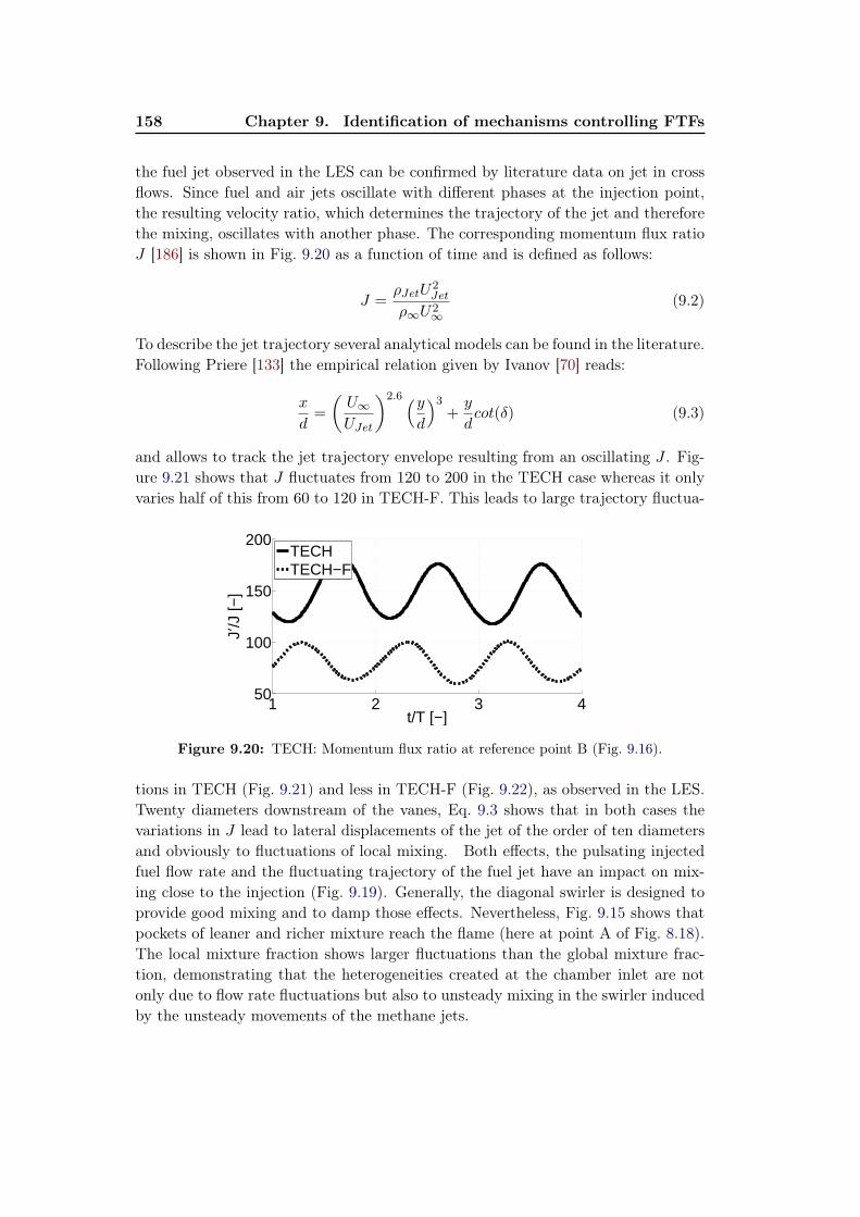
158 Chapter 9. Identification of mechanisms controlling FTFs
the fuel jet observed in the LES can be confirmed by literature data on jet in crossflows. Since fuel and air jets oscillate with different phases at the injection point,the resulting velocity ratio, which determines the trajectory of the jet and thereforethe mixing, oscillates with another phase. The corresponding momentum flux ratioJ [186] is shown in Fig. 9.20 as a function of time and is defined as follows:
J =ρJetU
2Jet
ρ∞U2∞
(9.2)
To describe the jet trajectory several analytical models can be found in the literature.Following Priere [133] the empirical relation given by Ivanov [70] reads:
x
d=
(U∞UJet
)2.6 (yd
)3+y
dcot(δ) (9.3)
and allows to track the jet trajectory envelope resulting from an oscillating J . Fig-ure 9.21 shows that J fluctuates from 120 to 200 in the TECH case whereas it onlyvaries half of this from 60 to 120 in TECH-F. This leads to large trajectory fluctua-
1 2 3 450
100
150
200
J′/J [−
]
t/T [−]
TECHTECH−F
Figure 9.20: TECH: Momentum flux ratio at reference point B (Fig. 9.16).
tions in TECH (Fig. 9.21) and less in TECH-F (Fig. 9.22), as observed in the LES.Twenty diameters downstream of the vanes, Eq. 9.3 shows that in both cases thevariations in J lead to lateral displacements of the jet of the order of ten diametersand obviously to fluctuations of local mixing. Both effects, the pulsating injectedfuel flow rate and the fluctuating trajectory of the fuel jet have an impact on mix-ing close to the injection (Fig. 9.19). Generally, the diagonal swirler is designed toprovide good mixing and to damp those effects. Nevertheless, Fig. 9.15 shows thatpockets of leaner and richer mixture reach the flame (here at point A of Fig. 8.18).The local mixture fraction shows larger fluctuations than the global mixture frac-tion, demonstrating that the heterogeneities created at the chamber inlet are notonly due to flow rate fluctuations but also to unsteady mixing in the swirler inducedby the unsteady movements of the methane jets.

9.2. Effects of mixture fluctuation 159
0 10 20 30 400
10
20
30
40
x/d [−]
y/d
[−
]
Phase I, III
Phase II
Phase IV
Figure 9.21: TECH: Jet trajectory envelope.
0 10 20 30 400
10
20
30
40
x/d [−]
y/d
[−
]
Phase I, III
Phase II
Phase IV
Figure 9.22: TECH-F: Jet trajectory envelope.
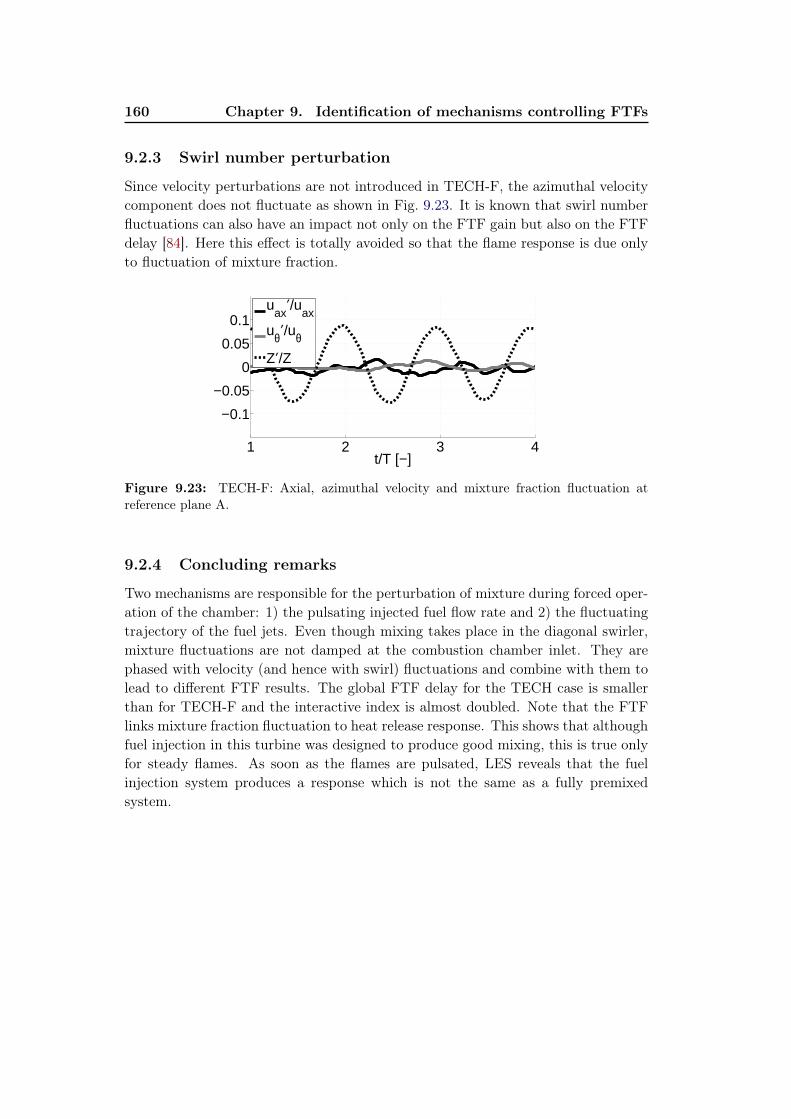
160 Chapter 9. Identification of mechanisms controlling FTFs
9.2.3 Swirl number perturbation
Since velocity perturbations are not introduced in TECH-F, the azimuthal velocitycomponent does not fluctuate as shown in Fig. 9.23. It is known that swirl numberfluctuations can also have an impact not only on the FTF gain but also on the FTFdelay [84]. Here this effect is totally avoided so that the flame response is due onlyto fluctuation of mixture fraction.
1 2 3 4
−0.1
−0.05
0
0.05
0.1
t/T [−]
uax
′/uax
uθ′/u
θ
Z′/Z
Figure 9.23: TECH-F: Axial, azimuthal velocity and mixture fraction fluctuation atreference plane A.
9.2.4 Concluding remarks
Two mechanisms are responsible for the perturbation of mixture during forced oper-ation of the chamber: 1) the pulsating injected fuel flow rate and 2) the fluctuatingtrajectory of the fuel jets. Even though mixing takes place in the diagonal swirler,mixture fluctuations are not damped at the combustion chamber inlet. They arephased with velocity (and hence with swirl) fluctuations and combine with them tolead to different FTF results. The global FTF delay for the TECH case is smallerthan for TECH-F and the interactive index is almost doubled. Note that the FTFlinks mixture fraction fluctuation to heat release response. This shows that althoughfuel injection in this turbine was designed to produce good mixing, this is true onlyfor steady flames. As soon as the flames are pulsated, LES reveals that the fuelinjection system produces a response which is not the same as a fully premixedsystem.
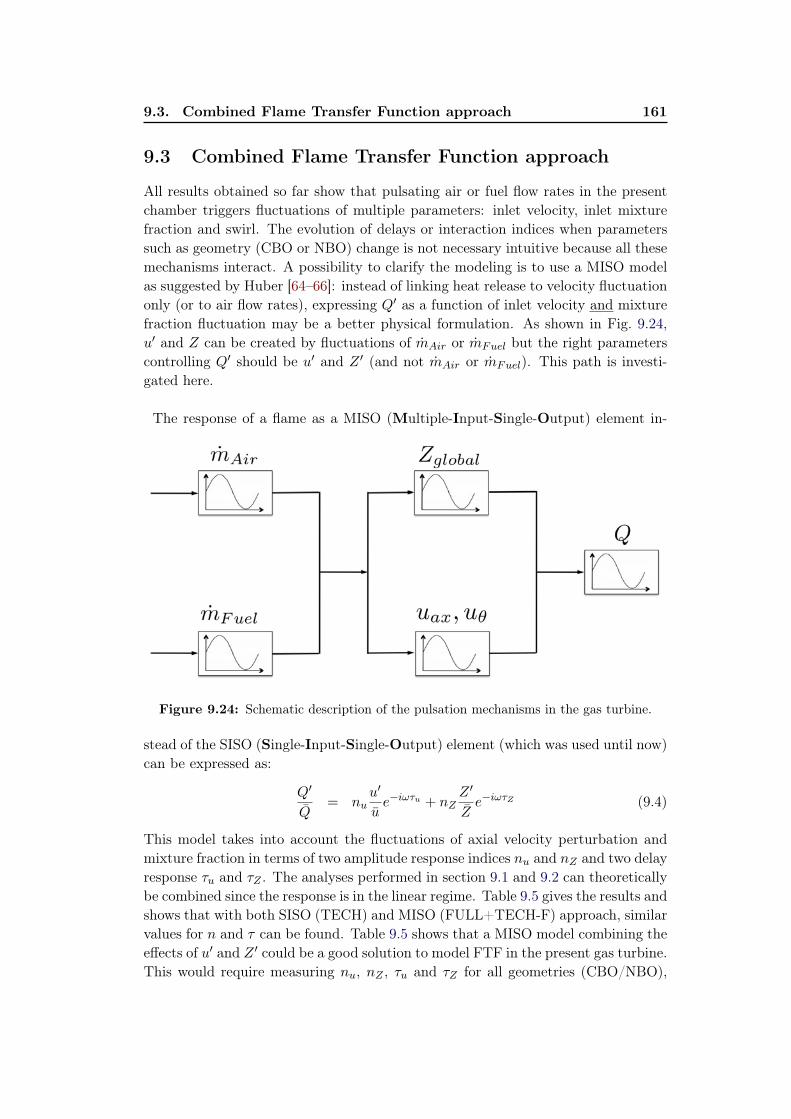
9.3. Combined Flame Transfer Function approach 161
9.3 Combined Flame Transfer Function approach
All results obtained so far show that pulsating air or fuel flow rates in the presentchamber triggers fluctuations of multiple parameters: inlet velocity, inlet mixturefraction and swirl. The evolution of delays or interaction indices when parameterssuch as geometry (CBO or NBO) change is not necessary intuitive because all thesemechanisms interact. A possibility to clarify the modeling is to use a MISO modelas suggested by Huber [64–66]: instead of linking heat release to velocity fluctuationonly (or to air flow rates), expressing Q′ as a function of inlet velocity and mixturefraction fluctuation may be a better physical formulation. As shown in Fig. 9.24,u′ and Z can be created by fluctuations of mAir or mFuel but the right parameterscontrolling Q′ should be u′ and Z ′ (and not mAir or mFuel). This path is investi-gated here.
The response of a flame as a MISO (Multiple-Input-Single-Output) element in-
Figure 9.24: Schematic description of the pulsation mechanisms in the gas turbine.
stead of the SISO (Single-Input-Single-Output) element (which was used until now)can be expressed as:
Q′
Q= nu
u′
ue−iωτu + nZ
Z ′
Ze−iωτZ (9.4)
This model takes into account the fluctuations of axial velocity perturbation andmixture fraction in terms of two amplitude response indices nu and nZ and two delayresponse τu and τZ . The analyses performed in section 9.1 and 9.2 can theoreticallybe combined since the response is in the linear regime. Table 9.5 gives the results andshows that with both SISO (TECH) and MISO (FULL+TECH-F) approach, similarvalues for n and τ can be found. Table 9.5 shows that a MISO model combining theeffects of u′ and Z ′ could be a good solution to model FTF in the present gas turbine.This would require measuring nu, nZ , τu and τZ for all geometries (CBO/NBO),
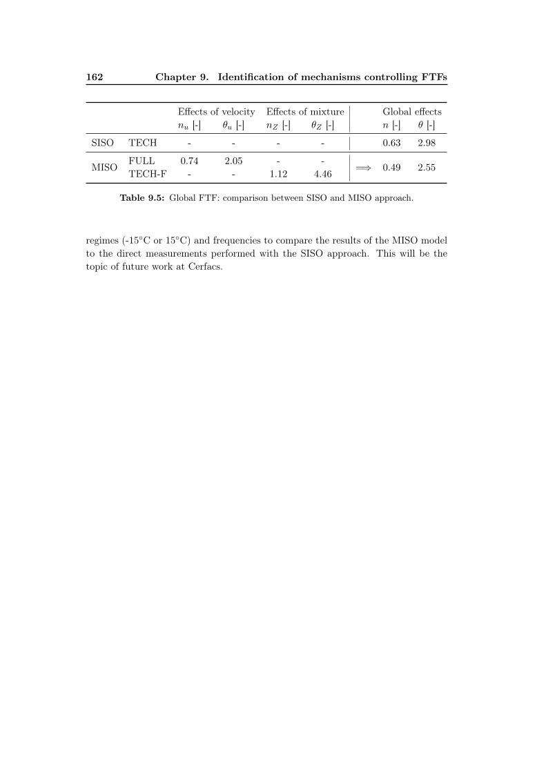
162 Chapter 9. Identification of mechanisms controlling FTFs
Effects of velocity Effects of mixture Global effectsnu [-] θu [-] nZ [-] θZ [-] n [-] θ [-]
SISO TECH - - - - 0.63 2.98
MISOFULL 0.74 2.05 - -
=⇒ 0.49 2.55TECH-F - - 1.12 4.46
Table 9.5: Global FTF: comparison between SISO and MISO approach.
regimes (-15◦C or 15◦C) and frequencies to compare the results of the MISO modelto the direct measurements performed with the SISO approach. This will be thetopic of future work at Cerfacs.

Chapter 10
Nonlinear analysis
Contents10.1 Mean pulsated flow fields . . . . . . . . . . . . . . . . . . . . . 165
10.2 Effect of pulsation amplitude on FDF . . . . . . . . . . . . . 170
10.2.1 Local Flame Transfer Function . . . . . . . . . . . . . . . . . 170
10.2.2 Mixture perturbation . . . . . . . . . . . . . . . . . . . . . . 172
10.3 Conclusion . . . . . . . . . . . . . . . . . . . . . . . . . . . . . 174
In the previous chapter, a possible extension of usual SISO (Single Input SingleOutput) models to MISO (Multiple Input Single Output) approaches have been dis-cussed. Another limitation of usual models is the existence of nonlinearities. Thisissue is investigated here for the gas turbine chamber.
For acoustically compact flames the linear analysis of combustion instabilities is gen-erally performed with the Flame Transfer Function (FTF) introduced by Crocco [29,30] presented in the previous chapters. In this approach the FTF is defined as therelative heat release fluctuation (q/q) to the relative inlet velocity perturbation(u/u) issued by the acoustic field and writes F (ω) = (q/q)/(u/u). Nevertheless it iswell known that in real gas turbine engines limit cycle oscillations can occur wherenon-linear effects play a dominant role. Figure 10.1 shows energy gain and lossesas a function of the perturbation in terms of the square of the acoustic velocity:the energy gain of the flame is linear for low perturbation amplitudes (region I)and saturates for larger perturbation levels (region II). The acoustic losses, e.g. dueto turbulence and the boundaries, are assumed to be linearly increasing with theperturbation level [35]. A limit cycle is reached when the losses and gain balance.This limit cycle is controlled by non-linear effects due to heat release [2, 3, 101].The flame is observed to saturate in the presence of high perturbation amplitudeswhen the acoustic velocity reaches a magnitude of the order of the mean flow veloc-ity [2, 3, 101, 118]. Since the flame response is not only a function of the frequencyany more but also of the perturbation amplitude, the classical FTF approach is notable to describe the flame behaviour correctly. Therefore an extended version ofthe linear FTF approach is introduced [35, 118]: The so-called Flame DescribingFunction (FDF) is defined as
F (ω, u) =q/q
u/u(10.1)
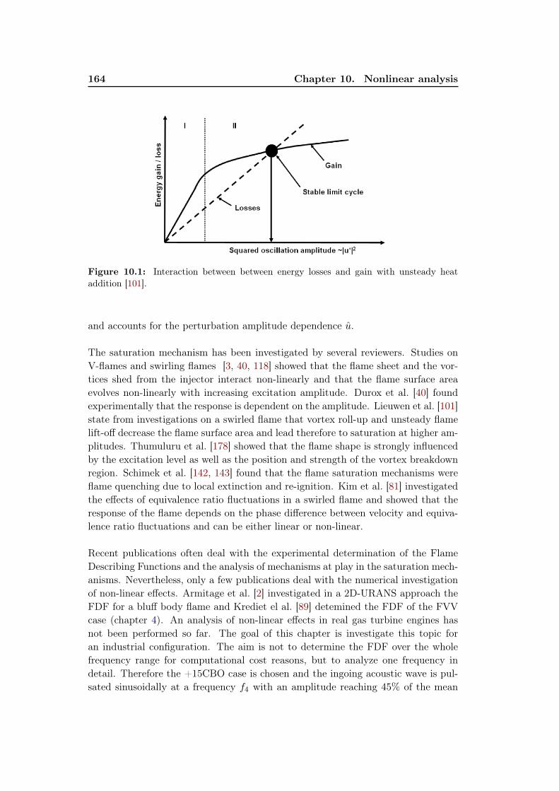
164 Chapter 10. Nonlinear analysis
Figure 10.1: Interaction between between energy losses and gain with unsteady heataddition [101].
and accounts for the perturbation amplitude dependence u.
The saturation mechanism has been investigated by several reviewers. Studies onV-flames and swirling flames [3, 40, 118] showed that the flame sheet and the vor-tices shed from the injector interact non-linearly and that the flame surface areaevolves non-linearly with increasing excitation amplitude. Durox et al. [40] foundexperimentally that the response is dependent on the amplitude. Lieuwen et al. [101]state from investigations on a swirled flame that vortex roll-up and unsteady flamelift-off decrease the flame surface area and lead therefore to saturation at higher am-plitudes. Thumuluru et al. [178] showed that the flame shape is strongly influencedby the excitation level as well as the position and strength of the vortex breakdownregion. Schimek et al. [142, 143] found that the flame saturation mechanisms wereflame quenching due to local extinction and re-ignition. Kim et al. [81] investigatedthe effects of equivalence ratio fluctuations in a swirled flame and showed that theresponse of the flame depends on the phase difference between velocity and equiva-lence ratio fluctuations and can be either linear or non-linear.
Recent publications often deal with the experimental determination of the FlameDescribing Functions and the analysis of mechanisms at play in the saturation mech-anisms. Nevertheless, only a few publications deal with the numerical investigationof non-linear effects. Armitage et al. [2] investigated in a 2D-URANS approach theFDF for a bluff body flame and Krediet el al. [89] detemined the FDF of the FVVcase (chapter 4). An analysis of non-linear effects in real gas turbine engines hasnot been performed so far. The goal of this chapter is investigate this topic foran industrial configuration. The aim is not to determine the FDF over the wholefrequency range for computational cost reasons, but to analyze one frequency indetail. Therefore the +15CBO case is chosen and the ingoing acoustic wave is pul-sated sinusoidally at a frequency f4 with an amplitude reaching 45% of the mean
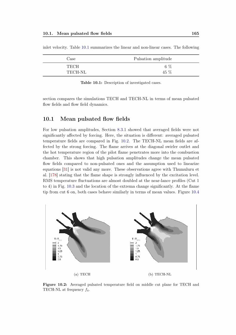
10.1. Mean pulsated flow fields 165
inlet velocity. Table 10.1 summarizes the linear and non-linear cases. The following
Case Pulsation amplitude
TECH 6 %TECH-NL 45 %
Table 10.1: Description of investigated cases.
section compares the simulations TECH and TECH-NL in terms of mean pulsatedflow fields and flow field dynamics.
10.1 Mean pulsated flow fields
For low pulsation amplitudes, Section 8.3.1 showed that averaged fields were notsignificantly affected by forcing. Here, the situation is different: averaged pulsatedtemperature fields are compared in Fig. 10.2. The TECH-NL mean fields are af-fected by the strong forcing. The flame arrives at the diagonal swirler outlet andthe hot temperature region of the pilot flame penetrates more into the combustionchamber. This shows that high pulsation amplitudes change the mean pulsatedflow fields compared to non-pulsated ones and the assumption used to linearizeequations [31] is not valid any more. These observations agree with Thumuluru etal. [178] stating that the flame shape is strongly influenced by the excitation level.RMS temperature fluctuations are almost doubled at the near-lance profiles (Cut 1
to 4) in Fig. 10.3 and the location of the extrema change significantly. At the flametip from cut 6 on, both cases behave similarly in terms of mean values. Figure 10.4
(a) TECH (b) TECH-NL
Figure 10.2: Averaged pulsated temperature field on middle cut plane for TECH andTECH-NL at frequency f4.

166 Chapter 10. Nonlinear analysis
shows the probability density functions (PDF) for the TECH and the TECH-NLflame in comparison to the unforced flame. Forcing has a strong influence on theequivalence ratio at which combustion takes place. For strong forcing (TECH-NL),the PDF of heat release versus equivalence ratio is flatter, indicating that moreflamelets are formed at equivalence ratios which differ from the mean value in thediagonal swirler. This shows that mixing is less efficient in the diagonal swirler forTECH-NL: strong forcing leads to less efficient mixing.
Phase averaging the PDF during the heat release oscillation cycle shows thatsignificant fluctuations of equivalence ratio occur (Fig. 10.5) for high forcing am-plitudes which are much less in the linear case. The phase averaged heat releaserate shows that the TECH-NL flame shape undergoes strong oscillation during theoscillation cycle, whereas the TECH flame shape is only slightly changing (Fig. 10.6to 10.9 for 2T to 3T/2). In TECH-NL at 2T , the flame rolls up at the lance anda "ball-like" structure with strong heat release rate appears along the inner flame.This structure grows within the oscillation cycle and decreases from T on. The max-imum of heat release along the inner flame is at T/2. At time T , the flame rolls-upat the tip and forms a characteristic "mushroom" shape. In TECH, the flame closeto the pilot injection is also characterized by a strong heat release but opens andcloses only slightly during T . A slightly higher heat release is also present along theinner flame front at T/2 which is due to a richer mixture entering this region. Theflame tip does not change significantly.
0 0.5−1
−0.8
−0.6
−0.4
−0.2
0
0.2
0.4
0.6
0.8
1
y/y
ma
x [
−]
1
0 0.5
2
0 0.5
3
0 0.5T
RMS/T
mean [−]
4
0 0.5
5
0 0.5
6
0 0.5
7
Non−pulsated
TECH
TECH−NL
Figure 10.3: Averaged RMS temperature profiles for the non-pulsated flame, TECH andTECH-NL.
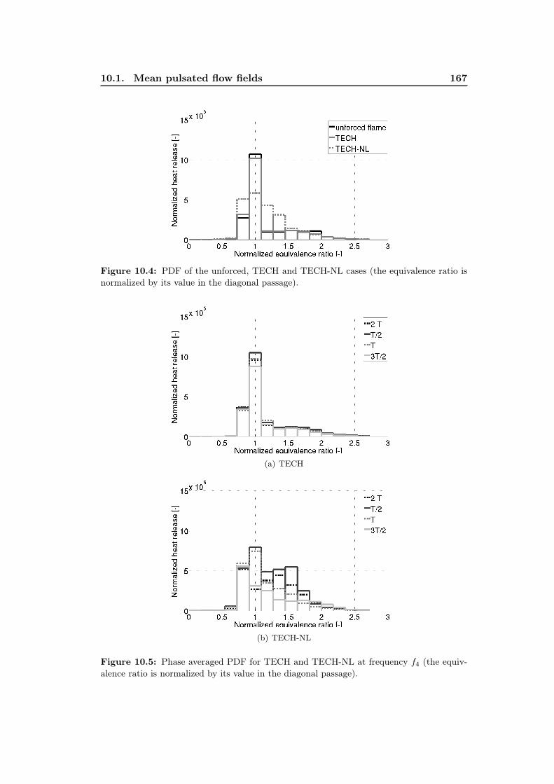
10.1. Mean pulsated flow fields 167
Figure 10.4: PDF of the unforced, TECH and TECH-NL cases (the equivalence ratio isnormalized by its value in the diagonal passage).
(a) TECH
(b) TECH-NL
Figure 10.5: Phase averaged PDF for TECH and TECH-NL at frequency f4 (the equiv-alence ratio is normalized by its value in the diagonal passage).

168 Chapter 10. Nonlinear analysis
(a) TECH (b) TECH-NL
Figure 10.6: Phase averaged pulsated heat release field on middle cut plane for TECHand TECH-NL at frequency f4 for 2T .
(a) TECH (b) TECH-NL
Figure 10.7: Phase averaged pulsated heat release field on middle cut plane for TECHand TECH-NL at frequency f4 for T/2.
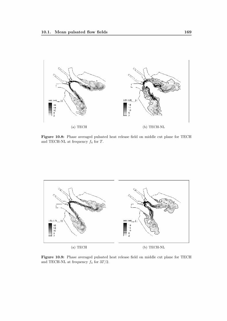
10.1. Mean pulsated flow fields 169
(a) TECH (b) TECH-NL
Figure 10.8: Phase averaged pulsated heat release field on middle cut plane for TECHand TECH-NL at frequency f4 for T .
(a) TECH (b) TECH-NL
Figure 10.9: Phase averaged pulsated heat release field on middle cut plane for TECHand TECH-NL at frequency f4 for 3T/2.
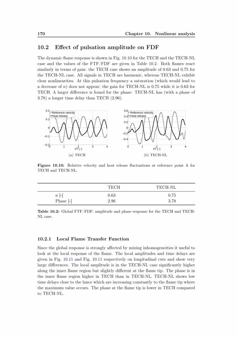
170 Chapter 10. Nonlinear analysis
10.2 Effect of pulsation amplitude on FDF
The dynamic flame response is shown in Fig. 10.10 for the TECH and the TECH-NLcase and the values of the FTF/FDF are given in Table 10.2. Both flames reactsimilarly in terms of gain: the TECH case shows an amplitude of 0.63 and 0.75 forthe TECH-NL case. All signals in TECH are harmonic, whereas TECH-NL exhibitclear nonlinearities. At this pulsation frequency a saturation (which would lead toa decrease of n) does not appear: the gain for TECH-NL is 0.75 while it is 0.63 forTECH. A larger difference is found for the phase: TECH-NL has (with a phase of3.78) a longer time delay than TECH (2.96).
0 1 2 3 4−0.2
−0.1
0
0.1
0.2
t/T [−]
Reference velocityHeat release
(a) TECH
0 1 2 3 4
−0.4
−0.2
0
0.2
0.4
0.6
t/T [−]
Reference velocityHeat release
(b) TECH-NL
Figure 10.10: Relative velocity and heat release fluctuations at reference point A forTECH and TECH-NL.
TECH TECH-NL
n [-] 0.63 0.75
Phase [-] 2.96 3.78
Table 10.2: Global FTF/FDF: amplitude and phase response for the TECH and TECH-NL case.
10.2.1 Local Flame Transfer Function
Since the global response is strongly affected by mixing inhomogeneities it useful tolook at the local response of the flame. The local amplitudes and time delays aregiven in Fig. 10.11 and Fig. 10.11 respectively on longitudinal cuts and show verylarge differences. The local amplitude is in the TECH-NL case significantly higheralong the inner flame region but slightly different at the flame tip. The phase is inthe inner flame region higher in TECH than in TECH-NL. TECH-NL shows lowtime delays close to the lance which are increasing constantly to the flame tip wherethe maximum value occurs. The phase at the flame tip is lower in TECH comparedto TECH-NL.
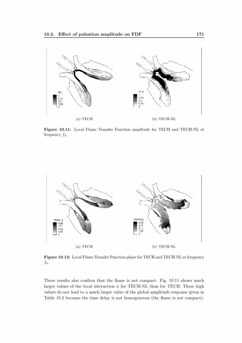
10.2. Effect of pulsation amplitude on FDF 171
(a) TECH (b) TECH-NL
Figure 10.11: Local Flame Transfer Function amplitude for TECH and TECH-NL atfrequency f4.
(a) TECH (b) TECH-NL
Figure 10.12: Local Flame Transfer Function phase for TECH and TECH-NL at frequencyf4.
These results also confirm that the flame is not compact: Fig. 10.11 shows muchlarger values of the local interaction n for TECH-NL than for TECH. These highvalues do not lead to a much larger value of the global amplitude response given inTable 10.2 because the time delay is not homogeneous (the flame is not compact).

172 Chapter 10. Nonlinear analysis
The link between the global amplitude n and the local field nl(~x) is:
ne−iωτ =
∫∫∫V
nl(~x)e−iωτl(~x) (10.2)
This relation is satisfied and it explains why n is not very different for TECH-NLcompared to TECH: local values of nl are larger for TECH-NL but since the flame isnot compact, these large nl values have opposite effects in regions where τl changesrapidly. In other words, at high pulsation amplitudes, the flame reacts locally morestrongly but this does not mean that the global amplification increases. The absenceof saturation observed at high amplitudes of the flame is only true for the globalFTF. Locally, the gain increases with increasing velocity perturbation.
10.2.2 Mixture perturbation
The perturbation of mixture results from the fluctuating inlet air mass flow rate(Fig. 10.13) which causes the fuel flow rate to oscillate (20%) in TECH-NL. Theglobal mixture fraction fluctuation is much larger for TECH-NL (Z ′/Z between−0.4 and 3.8) compared to TECH (Z ′/Z = ±0.1) as shown by Fig. 10.14 which alsoshows nonlinear variations of Z ′ for TECH-NL. Further downstream at the referenceplane A (Fig. 10.15), the fluctuations in TECH-NL are damped to about 10% (be-tween −0.33 and 0.4), whereas TECH fluctuates with 50% of the inlet fluctuations(Z ′/Z = ±0.05). Higher mixture fraction fluctuation are also stronger damped inthe swirler. The nonlinear oscillation in TECH-NL explains also the nonlinear heatrelease fluctuation. At strong forcing levels the fluctuations of equivalence ratio atthe chamber inlet are very strong: it is likely for example that when Z ′/Z reaches−0.3, the mixture gets out of flammability limits and must mix downstream of thechamber inlet before burning.
0 1 2 3 4−1
−0.5
0
0.5
1
t/T [−]
m’Fuel
/ mFuel
[−]
m’Air
/ mAir
[−]
Figure 10.13: Air and fuel mass flow rate fluctuation at the diagonal swirler inlet forTECH-NL.

10.2. Effect of pulsation amplitude on FDF 173
0 1 2 3 4−0.4
−0.2
0
0.2
0.4
Z′/Z
[−
]
t/T [−]
TECHTECH−NL
Figure 10.14: Relative mixture fraction fluctuation at the diagonal swirler inlet for TECHand TECH-NL.
0 1 2 3 4−2
0
2
4
Z′/Z
[−
]
t/T [−]
TECHTECH−NL
Figure 10.15: Relative mixture fraction fluctuation at the reference plane A for TECHand TECH-NL.
174 Chapter 10. Nonlinear analysis
10.3 Conclusion
The pulsation with high excitation level created for the TECH-NL run causes anon-linear response of the flame. The averaged flame shape changes significantlycompared to the linear behaviour. During the oscillation cycle the flame undergoesstrong variations in shape, with a typical roll-up in mushroom shape [123]. Theglobal FTF shows that the forcing amplitude does not only lead to a saturationof the flame [2, 3, 101, 118] but also changes the delay response. The heat releaseoscillation shows sharp peaks at its maximum which could be related to the mixturefraction fluctuation. Strong fluctuations of equivalence ratio during the oscillationcycle are shown by PDFs. Local FTF fields reveal that the local interaction indexincreases significantly with increasing forcing amplitude. Nevertheless the globalgain remains similar between the linear and non-linear case since the flame is notcompact. This means that high local gain values have opposite effects in regionswhere the local time delay changes rapidly. To conclude, forcing amplitudes do havean influence on the FTF when they reach large values. Whether this point must beincluded now in the analysis of instabilities in this gas turbine is an open question:the forcing amplitude used in TECH-NL was very large and should not be reachedin the real engine. Moreover, ensuring linear stability (for which linear FTFs aresufficient) is a priority for engineering purposes. However, moving from FTF to FDFformulation is clearly an interesting path which will be investigated in the future.
Conclusion and perspectives
"The machine does not isolate man from the great problems of naturebut plunges him more deeply into them." Antoine de Saint-Exupery(1900-1944).
Modern pollutant regulations have led to lean (technically) premixed combustionsystems which are prone to thermo-acoustic instabilities. In this work, compressiblereactive Large Eddy Simulation (LES) has been applied to an academic single burnerand a heavy-duty industrial gas turbine combustion chamber. The coupling betweenacoustic and combustion has been modeled with the Flame Transfer Function ap-proach. The LES of the academic burner has been successfully validated againstmeasurements and against OpenFoam LES simulations. The large-scale industrialgas turbine has been analyzed for two different burner geometries and operatingconditions. The assumption used to linearize equations is valid in the linear regimeas mean flow fields with forcing remained similar to the unforced mean fields whichis not valid for high pulsation amplitudes in the nonlinear regime. The FTF wasonly slightly influenced for the two operating points considered here. Burner outletsdid modify the characteristics of the FTF with the Cylindrical Burner Outlet (CBO)cases having a slightly shorter time lag than the cases without elongated burner out-let (NBO) whereas the CBO flames were slightly longer. This means that a simplemodel taking only into account the flight time from the reference point to the flameis not appropriate and additional mechanisms are at play.
Results showed that pulsating air or fuel flow rates trigger fluctuations of the in-let velocity, swirl and the inlet mixture fraction whereas the latter is caused by twomechanisms: 1) the pulsating injected fuel flow rate and 2) the fluctuating trajectoryof the fuel jets. The diagonal swirler, although designed to provide good mixing, didnot damp those effects at the combustion chamber inlet. Mixing inhomogeneitiesshowed to partially control the FTF delay which gets shorter in their absence whena fully premixed flow passes the diagonal swirler instead. Mixture perturbations arephased with velocity (and hence with swirl) fluctuations and combine with themto lead to different FTF results. Another possibility to clarify modeling of FTFs islinking heat release to inlet velocity and mixture fraction fluctuation (MISO model)which showed to be a promising solution. The nonlinear analysis showed that theforcing amplitude not only leads to a saturation of the flame but also to changes ofthe delay response. All flames studied here were not compact: flame regions locatedright next to each other exhibited significant differences in delay meaning that atthe same instant certain parts of the flame damp the excitation while others feed it.
The ability of LES to handle complex unsteady phenomena in gas turbines hasbeen evidenced during this thesis work. LES has shown its ability to give importantinsight in the mechanisms dominating the dynamic flame behaviour. Embedding

176 Conclusion and perspectives
LES solvers at an early design stage is recommended to help understanding andchanging flame dynamics in order to finally construct stable combustors.
Thermo-acoustic instabilities are mainly controlled by the complex interaction be-tween acoustics and combustion. Future work includes further evaluating the effectsof combustion modeling and chemical kinetics on the dynamic flame behaviour. Alsothe influence of a more detailed chemical reaction scheme should be evaluated inorder to predict pollutant emissions. Furthermore, the influence of cooling of thechamber walls has not been investigated in this work and should be considered forthe future. Including further details in the LES is a logical step since computationalpower is increasing continuously.
List of Figures
1.1 Population of the world, 1950-2100, according to different projectionsand variants [111]. . . . . . . . . . . . . . . . . . . . . . . . . . . . . 4
1.2 World energy consumption and projection [99]. . . . . . . . . . . . . 41.3 Temperature deviations over the pas millenia [72]. . . . . . . . . . . . 61.4 Fossil fuel resources estimation for different world regions [184]. . . . 61.5 Chimney jack from Da Vinci. . . . . . . . . . . . . . . . . . . . . . . 71.6 Siemens gas turbine. Model V84.3A/V94.3A. (www.siemens.com). . 81.7 Brayton cycle in a gas turbine: P-v and T-s diagram. . . . . . . . . . 91.8 Combustion chamber designs. (Source: The jet engine , Rolls-Royce
plc.) . . . . . . . . . . . . . . . . . . . . . . . . . . . . . . . . . . . . 9
2.1 Feedback mechanism responsible for combustion instabilities [103]. . 162.2 Interaction between between energy losses and gain with unsteady
heat addition [101]. . . . . . . . . . . . . . . . . . . . . . . . . . . . . 182.3 Growth of a combustion instability to limit cycle [126]. . . . . . . . . 182.4 Forced (left) and self-excited (right) strategies to study thermo-acoustic
instabilities [126]. . . . . . . . . . . . . . . . . . . . . . . . . . . . . . 202.5 Decaying eigenvectors in a normal (a) and non-normal (b) system. . 262.6 Schematic drawing of self-excited and forced response method. . . . . 28
3.1 Conceptual differences between DNS, LES and RANS. . . . . . . . . 333.2 Direct Numerical Simulation of flame/turbulence interaction [126]. . 353.3 Typical velocity profile near the wall and notation used for near-wall
quantities [145]. . . . . . . . . . . . . . . . . . . . . . . . . . . . . . . 393.4 System identification: Black box. . . . . . . . . . . . . . . . . . . . . 413.5 System identification process with Wiener-Hopf (adapted from [176]). 43
4.1 Experimental test rig [143] . . . . . . . . . . . . . . . . . . . . . . . . 484.2 Cross-section of swirler, annular duct and combustion chamber [142]. 494.3 Mesh and computational domain . . . . . . . . . . . . . . . . . . . . 50
5.1 Instantaneous axial velocity field on middle cut plane and tempera-ture iso-surface (T = 1200 K). . . . . . . . . . . . . . . . . . . . . . . 54
5.2 Averaged axial velocity field on middle cut plane. . . . . . . . . . . . 545.3 Temperature field on middle cut plane. . . . . . . . . . . . . . . . . . 555.4 Heat release field on middle cut plane. . . . . . . . . . . . . . . . . . 555.5 Reference plane for FTF determination, location of cuts at ∆x =
0.01, 0.02, 0.03, 0.04, 0.05 and 0.1 m and iso-line of temperature (T =
1200 K). . . . . . . . . . . . . . . . . . . . . . . . . . . . . . . . . . . 565.6 Temperature profiles at x = 0.01, 0.02, 0.03, 0.04, 0.05 and 0.1 m for
AVBP and OpenFoam. . . . . . . . . . . . . . . . . . . . . . . . . . . 57
178 List of Figures
5.7 Axial velocity profiles at x = 0.01, 0.02, 0.03, 0.04, 0.05 and 0.1 m forAVBP, OpenFoam and PIV. . . . . . . . . . . . . . . . . . . . . . . . 57
5.8 Radial veloctiy profiles at x = 0.01, 0.02, 0.03, 0.04, 0.05 and 0.1 mfor AVBP, OpenFoam and PIV. . . . . . . . . . . . . . . . . . . . . . 58
5.9 Tangential veloctiy profiles at x = 0.01, 0.02, 0.03, 0.04, 0.05 and 0.1
m for AVBP and OpenFoam. . . . . . . . . . . . . . . . . . . . . . . 585.10 RMS temperature profiles at x = 0.01, 0.02, 0.03, 0.04, 0.05 and 0.1 m
for AVBP and OpenFoam. . . . . . . . . . . . . . . . . . . . . . . . . 595.11 Comparison of Flame Transfer Function obtained with AVBP, Open-
Foam and measurements. . . . . . . . . . . . . . . . . . . . . . . . . 605.12 Phase averaged temperature field for 115 Hz and iso-line of heat re-
lease (the level of the isoline corresponds to the mean heat releaseover the whole cycle). . . . . . . . . . . . . . . . . . . . . . . . . . . 61
5.13 Illustration of the creation of swirl number perturbations. . . . . . . 625.14 Normalised axial, transverse velocity and swirl fluctuation at the ref-
erence plane for a forcing frequency of 53 Hz. . . . . . . . . . . . . . 635.15 Normalised axial, transverse velocity and swirl fluctuation at the ref-
erence plane for a forcing frequency of 115 Hz. . . . . . . . . . . . . . 63
6.1 3D view (left) of the annular combustion chamber. One sector (right)will be used for LES here. . . . . . . . . . . . . . . . . . . . . . . . . 68
6.2 Burner details . . . . . . . . . . . . . . . . . . . . . . . . . . . . . . . 696.3 Burner outlet details. . . . . . . . . . . . . . . . . . . . . . . . . . . . 696.4 The single sector setup is installed in Italy on a laboratory chamber. 706.5 Mesh used for the real gas turbine. . . . . . . . . . . . . . . . . . . . 726.6 Mesh used for the experimental test rig. . . . . . . . . . . . . . . . . 736.7 Laminar flame speed s0
L vs. equivalence ratio φ at 300 K and 1 bar [155]. 756.8 Comparison between GRI-meach and BFER scheme for (a) different
pressures p = 1, 3, 10atm at T = 300K and (b)different temperaturesT = 300, 500, 700K at p = 1atm [45]. . . . . . . . . . . . . . . . . . . 76
6.9 Temperature over equivalence ratio for GRI-Mech and BFER forCH4/air flames at T = 700 K and p = 17 bar. . . . . . . . . . . . . . 77
6.10 Laminar flame speed over equivalence ratio for GRI-Mech and BFERfor CH4/air flames at T = 700 K and p = 17 bar. . . . . . . . . . . . 77
7.1 Precessing vortex core (PVC) in cold flow LES. . . . . . . . . . . . . 817.2 Mean axial velocity field on middle cut plane. The white line corre-
sponds to zero axial velocity. . . . . . . . . . . . . . . . . . . . . . . 827.3 Reference plane location. . . . . . . . . . . . . . . . . . . . . . . . . . 827.4 Axial-velocity: comparison PIV and LES. . . . . . . . . . . . . . . . 837.5 y-velocity: comparison PIV and LES. . . . . . . . . . . . . . . . . . . 837.6 z-velocity: comparison PIV and LES. . . . . . . . . . . . . . . . . . . 847.7 Tangential velocity: comparison PIV and LES. . . . . . . . . . . . . 847.8 Total pressure field on middle cut plane. . . . . . . . . . . . . . . . . 86
List of Figures 179
7.9 Instantaneous iso-surface of Q-criterion (Q = 3.4·108) in the chamber.Case +15CBO and +15NBO. . . . . . . . . . . . . . . . . . . . . . . 88
7.10 Normalized axial velocity field on middle cut plane and iso-line ofzero axial velocity (solid black line). . . . . . . . . . . . . . . . . . . 89
7.11 Planes for profile extraction . . . . . . . . . . . . . . . . . . . . . . . 907.12 Axial velocity profiles for +15CBO, +15NBO, -15CBO, -15NBO . . 907.13 Radial velocity profiles for +15CBO, +15NBO, -15CBO, -15NBO . . 927.14 Tangential velocity profiles for +15CBO, +15NBO, -15CBO, -15NBO 927.15 Temperature iso-surface (T/Tmean = 1.3) coloured by normalized ax-
ial velocity. . . . . . . . . . . . . . . . . . . . . . . . . . . . . . . . . 937.16 Normalized temperature field on middle cut plane. . . . . . . . . . . 947.17 Temperature profiles for +15CBO, +15NBO, -15CBO, -15NBO . . . 957.18 RMS temperature profiles for +15CBO, +15NBO, -15CBO, -15NBO 957.19 Normalized RMS pressure field on middle cut plane obtained from
LES data. . . . . . . . . . . . . . . . . . . . . . . . . . . . . . . . . . 967.20 FFT of chamber pressure signal and heat release rate obtained from
LES data. . . . . . . . . . . . . . . . . . . . . . . . . . . . . . . . . . 977.21 Mode shape obtained with the Helmholtz 3D solver AVSP. . . . . . . 977.22 Instantaneous temperature field close to the lance. . . . . . . . . . . 1007.23 Temperature iso-line (T/Tmean = 1.3) and pressure iso-surface (vi-
sualizing the PVC structure) for the -15CBO case: attached (a) anddetached (b) flame. The PVC disappears totally for the attached flame.102
7.24 Temperature iso-surface (T/Tmean = 1.3) coloured by normalized ax-ial velocity for the -15CBO case: attached (a) and detached (b) flame. 102
7.25 Detached flame (-15CBO-D). . . . . . . . . . . . . . . . . . . . . . . 1037.26 Axial velocity profiles for the attached (-15CBO) and detached (-
15CBO-D) flame. . . . . . . . . . . . . . . . . . . . . . . . . . . . . . 1047.27 Radial velocity profiles for the attached (-15CBO) and detached (-
15CBO-D) flame. . . . . . . . . . . . . . . . . . . . . . . . . . . . . . 1047.28 Tangential velocity profiles for the attached (-15CBO) and detached
(-15CBO-D) flame. . . . . . . . . . . . . . . . . . . . . . . . . . . . . 1057.29 Temperature profiles for the attached (-15CBO) and detached (-15CBO-
D) flame. . . . . . . . . . . . . . . . . . . . . . . . . . . . . . . . . . 1057.30 RMS temperature profiles for the attached (-15CBO) and detached
flame (-15CBO-D) . . . . . . . . . . . . . . . . . . . . . . . . . . . . 1067.31 Thickening factor on the middle cut plane (+15CBO). . . . . . . . . 1077.32 Turbulent viscosity ratio on the middle cut plane (+15CBO). . . . . 1077.33 PDF of thickening factor (+15CBO). . . . . . . . . . . . . . . . . . . 108
8.1 Reference point location for FTF measurement and pulsation procedure.1128.2 Typical time evolution of heat release rate and velocity fluctuation at
the reference point A (Fig. 8.1). . . . . . . . . . . . . . . . . . . . . . 1138.3 Flame Transfer Function for +15CBO. . . . . . . . . . . . . . . . . . 1148.4 Flame Transfer Function for +15NBO. . . . . . . . . . . . . . . . . . 115
180 List of Figures
8.5 Flame Transfer Function for -15CBO. . . . . . . . . . . . . . . . . . 1158.6 Flame Transfer Function for -15NBO. . . . . . . . . . . . . . . . . . 1168.7 +15CBO: Temperature profiles for the averaged pulsated and non-
pulsated flame at f4. . . . . . . . . . . . . . . . . . . . . . . . . . . . 1198.8 +15CBO: Axial velocity profiles for the averaged pulsated and non-
pulsated flame at f4. . . . . . . . . . . . . . . . . . . . . . . . . . . . 1208.9 +15CBO: RMS temperature profiles for the averaged pulsated and
non-pulsated flame at f4. . . . . . . . . . . . . . . . . . . . . . . . . 1208.10 +15NBO: Temperature profiles for the averaged pulsated and non-
pulsated flame at f4. . . . . . . . . . . . . . . . . . . . . . . . . . . . 1218.11 +15NBO: RMS temperature profiles for the averaged pulsated and
non-pulsated flame at f4 (+15NBO). . . . . . . . . . . . . . . . . . . 1218.12 Flame response and velocity signal for +15CBO, +15NBO, -15CBO
and -15NBO at f4. . . . . . . . . . . . . . . . . . . . . . . . . . . . . 1228.13 Local amplitude response for the cases +15CBO, +15NBO, -15CBO
and -15NBO at frequency f4. . . . . . . . . . . . . . . . . . . . . . . 1248.14 Local phase response for the cases +15CBO, +15NBO, -15CBO and
-15NBO at frequency f4. . . . . . . . . . . . . . . . . . . . . . . . . . 1258.15 Normalized equivalence ratio field and iso-line of heat release rate on
the middle cut plane for +15CBO and +15NBO at T/2 and 3T/2phase averaged over the heat release oscillation cycle. . . . . . . . . . 127
8.16 Local amplitude response for +15CBO at frequencies f1, f2, f3 and f4.1308.17 Local phase response for +15CBO at frequencies f1, f2, f3 and f4. . 1318.18 Location of reference point A, plane A and reference point C. . . . . 1328.19 Relative variations of the air mass flow rate at diagonal inlet at fre-
quencies f1, f2, f3 and f4. . . . . . . . . . . . . . . . . . . . . . . . . 1338.20 Relative variations of the fuel mass flow rate at diagonal inlet at
frequencies f1, f2, f3 and f4. . . . . . . . . . . . . . . . . . . . . . . 1338.21 Global mixture fraction (Eq. 8.5) at diagonal inlet for frequencies f1,
f2, f3 and f4. . . . . . . . . . . . . . . . . . . . . . . . . . . . . . . . 1348.22 Global mixture fraction averaged over reference plane A for frequen-
cies f1, f2, f3 and f4. . . . . . . . . . . . . . . . . . . . . . . . . . . . 1348.23 Normalized equivalence ratio field and iso-line of heat release rate on
the middle cut plane for +15CBO phase averaged at the maximumof the heat release oscillation cycle for frequencies f1, f2, f3 and f4. . 135
8.24 Normalized equivalence ratio field and iso-line of heat release rate onthe middle cut plane for +15CBO phase averaged at the minimum ofthe heat release oscillation cycle for frequencies f1, f2, f3 and f4. . . 136
8.25 Relative axial velocity, mixture fraction and heat release fluctuationat reference point C for frequency f1. . . . . . . . . . . . . . . . . . . 137
8.26 Relative axial velocity, mixture fraction and heat release fluctuationat reference point C for frequency f2. . . . . . . . . . . . . . . . . . . 137
8.27 Relative axial velocity, mixture fraction and heat release fluctuationat reference point C for frequency f3. . . . . . . . . . . . . . . . . . . 138
List of Figures 181
8.28 Relative axial velocity, mixture fraction and heat release fluctuationat reference point C for frequency f4. . . . . . . . . . . . . . . . . . . 138
8.29 Illustration of the propagation of swirl number and mixture pertur-bations. . . . . . . . . . . . . . . . . . . . . . . . . . . . . . . . . . . 139
8.30 Relative fluctuation of axial velocity u′ax/uax, azimuthal velocity u′θ/uθand mixture fraction Z ′/Z at reference plane A for frequency f1. . . 140
8.31 Relative fluctuation of axial velocity u′ax/uax, azimuthal velocity u′θ/uθand mixture fraction Z ′/Z at reference plane A for frequency f2. . . 140
8.32 Relative fluctuation of axial velocity u′ax/uax, azimuthal velocity u′θ/uθand mixture fraction Z ′/Z at reference plane A for frequency f3. . . 141
8.33 Relative fluctuation of axial velocity u′ax/uax, azimuthal velocity u′θ/uθand mixture fraction Z ′/Z at reference plane A for frequency f4. . . 141
9.1 Schematic description of the pulsation mechanisms in the gas turbine.In previous chapters, mAir and mFuel were both pulsated. Here, onlyone will be pulsated for each case. . . . . . . . . . . . . . . . . . . . . 144
9.2 Schematic description of the pulsation mechanisms in the gas turbinewith a fully premixed diagonal swirler. Only the inlet velocity u
changes. . . . . . . . . . . . . . . . . . . . . . . . . . . . . . . . . . . 1459.3 Normalized averaged equivalence ratio field and temperature iso-line
for the TECH (left) and the FULL (right) case. . . . . . . . . . . . . 1469.4 Profiles of temperature for the pulsated mean technically (TECH)
and fully premixed flame (FULL). . . . . . . . . . . . . . . . . . . . 1479.5 Profiles of RMS temperature for the pulsated mean technically (TECH)
and fully premixed flame (FULL). . . . . . . . . . . . . . . . . . . . 1479.6 PDF of the TECH and the FULL case for the averaged and the
pulsated averaged flame (the equivalence ratio is normalized by itsvalue in the diagonal passage). . . . . . . . . . . . . . . . . . . . . . 148
9.7 Relative velocity perturbation at the reference point A and relativeheat release fluctuation for the TECH and the FULL cases (frequencyf4). . . . . . . . . . . . . . . . . . . . . . . . . . . . . . . . . . . . . . 149
9.8 Amplitude of the local FTF for the TECH (left) and the FULL case(right). . . . . . . . . . . . . . . . . . . . . . . . . . . . . . . . . . . . 151
9.9 Time delay of the local FTF for the TECH (left) and the FULL case(right). . . . . . . . . . . . . . . . . . . . . . . . . . . . . . . . . . . . 151
9.10 Schematic description of the pulsation mechanisms in the gas turbinewith only fuel fluctuation. Only the inlet mixture fraction changes(TECH-F). . . . . . . . . . . . . . . . . . . . . . . . . . . . . . . . . 152
9.11 Normalized mixture fraction at the reference plane A (Fig. 8.18) andheat release rate for TECH. . . . . . . . . . . . . . . . . . . . . . . . 153
9.12 Normalized mixture fraction at the reference plane A (Fig. 8.18) andheat release rate for TECH-F. . . . . . . . . . . . . . . . . . . . . . . 153
9.13 Global mixture fraction at diagonal swirler inlet for TECH, TECH-Fand mean diagonal mixture fraction. . . . . . . . . . . . . . . . . . . 155

182 List of Figures
9.14 Spatially averaged mixture fraction at reference plane A (Fig. 8.18)for TECH, TECH-F and mean diagonal mixture fraction. . . . . . . 155
9.15 Local mixture fraction at the reference point A (Fig. 8.18) for TECH,TECH-F and mean diagonal mixture fraction. . . . . . . . . . . . . . 155
9.16 Relative fuel and air velocity at reference point B. . . . . . . . . . . 1569.17 TECH: Relative fuel and air velocity perturbation at reference point
B (Fig. 9.16). . . . . . . . . . . . . . . . . . . . . . . . . . . . . . . . 1569.18 TECH-F: Relative fuel and air velocity perturbation at reference
point B (Fig. 9.16). . . . . . . . . . . . . . . . . . . . . . . . . . . . . 1579.19 Jet trajectory visualized as YCH4 iso-surface and normalized equiva-
lence ratio field for two distinct snapshots (TECH case). . . . . . . . 1579.20 TECH: Momentum flux ratio at reference point B (Fig. 9.16). . . . . 1589.21 TECH: Jet trajectory envelope. . . . . . . . . . . . . . . . . . . . . . 1599.22 TECH-F: Jet trajectory envelope. . . . . . . . . . . . . . . . . . . . . 1599.23 TECH-F: Axial, azimuthal velocity and mixture fraction fluctuation
at reference plane A. . . . . . . . . . . . . . . . . . . . . . . . . . . . 1609.24 Schematic description of the pulsation mechanisms in the gas turbine. 161
10.1 Interaction between between energy losses and gain with unsteadyheat addition [101]. . . . . . . . . . . . . . . . . . . . . . . . . . . . . 164
10.2 Averaged pulsated temperature field on middle cut plane for TECHand TECH-NL at frequency f4. . . . . . . . . . . . . . . . . . . . . . 165
10.3 Averaged RMS temperature profiles for the non-pulsated flame, TECHand TECH-NL. . . . . . . . . . . . . . . . . . . . . . . . . . . . . . . 166
10.4 PDF of the unforced, TECH and TECH-NL cases (the equivalenceratio is normalized by its value in the diagonal passage). . . . . . . . 167
10.5 Phase averaged PDF for TECH and TECH-NL at frequency f4 (theequivalence ratio is normalized by its value in the diagonal passage). 167
10.6 Phase averaged pulsated heat release field on middle cut plane forTECH and TECH-NL at frequency f4 for 2T . . . . . . . . . . . . . . 168
10.7 Phase averaged pulsated heat release field on middle cut plane forTECH and TECH-NL at frequency f4 for T/2. . . . . . . . . . . . . 168
10.8 Phase averaged pulsated heat release field on middle cut plane forTECH and TECH-NL at frequency f4 for T . . . . . . . . . . . . . . . 169
10.9 Phase averaged pulsated heat release field on middle cut plane forTECH and TECH-NL at frequency f4 for 3T/2. . . . . . . . . . . . . 169
10.10Relative velocity and heat release fluctuations at reference point Afor TECH and TECH-NL. . . . . . . . . . . . . . . . . . . . . . . . . 170
10.11Local Flame Transfer Function amplitude for TECH and TECH-NLat frequency f4. . . . . . . . . . . . . . . . . . . . . . . . . . . . . . . 171
10.12Local Flame Transfer Function phase for TECH and TECH-NL atfrequency f4. . . . . . . . . . . . . . . . . . . . . . . . . . . . . . . . 171
10.13Air and fuel mass flow rate fluctuation at the diagonal swirler inletfor TECH-NL. . . . . . . . . . . . . . . . . . . . . . . . . . . . . . . 172
List of Figures 183
10.14Relative mixture fraction fluctuation at the diagonal swirler inlet forTECH and TECH-NL. . . . . . . . . . . . . . . . . . . . . . . . . . . 173
10.15Relative mixture fraction fluctuation at the reference plane A forTECH and TECH-NL. . . . . . . . . . . . . . . . . . . . . . . . . . . 173

List of Tables
3.1 Reflection coefficients of the boundary conditions used in this thesis. 37
4.1 Main parameters of the FVV configuration. . . . . . . . . . . . . . . 484.2 Operating point . . . . . . . . . . . . . . . . . . . . . . . . . . . . . . 504.3 Parameters describing the mesh for the FVV burner. . . . . . . . . . 504.4 Numerical parameters used for the FVV simulation. . . . . . . . . . 524.5 Coefficients used in the reduced chemical scheme for CH4/air flames. 52
6.1 Parameters describing the mesh for the real gas turbine. . . . . . . . 716.2 Parameters describing the grid for the experimental test rig. . . . . . 716.3 Investigated cases . . . . . . . . . . . . . . . . . . . . . . . . . . . . . 746.4 Numerical parameters used for the real gas turbine simulation. . . . 786.5 Numerical parameters used for the experimental non reacting test rig
simulation of Genoa. . . . . . . . . . . . . . . . . . . . . . . . . . . . 78
7.1 Ratio SLESe /SExpe of the computed equivalent section to the experi-mental value. . . . . . . . . . . . . . . . . . . . . . . . . . . . . . . . 85
7.2 Denomination of investigated cases. . . . . . . . . . . . . . . . . . . . 877.3 Flame stabilization: Wall treatment at the lance . . . . . . . . . . . 997.4 Nomenclature for attached and detached flame. . . . . . . . . . . . . 101
8.1 FTF determination: amplitude n and phase θ. . . . . . . . . . . . . . 1148.2 Global FTF: amplitude n and phase θ for +15CBO, +15NBO, -
15CBO and -15NBO at f4. . . . . . . . . . . . . . . . . . . . . . . . 1238.3 Comparison between local (obtained by Eq. 8.2) and global FTF (ob-
tained by Eq. 10.1). . . . . . . . . . . . . . . . . . . . . . . . . . . . 1248.4 Global FTF: amplitude n and phase θ for +15CBO at f1, f2, f3 and
f4. . . . . . . . . . . . . . . . . . . . . . . . . . . . . . . . . . . . . . 1298.5 Phase angle (radian) of mixture fraction and axial velocity to the heat
release rate oscillation at reference point C for f1, f2, f3 and f4. . . . 138
9.1 Description of investigated cases: TECH and FULL. Both cases cor-respond to +15CBO. . . . . . . . . . . . . . . . . . . . . . . . . . . . 145
9.2 Global FTF: amplitude n and phase θ for TECH and FULL. . . . . 1499.3 Description of investigated cases: TECH and TECH-F . . . . . . . . 1529.4 Global FTF: amplitude n and phase θ for TECH and TECH-F based
on reference plane A (Fig. 8.18) and mixture fraction fluctuation(Eq. 9.1). . . . . . . . . . . . . . . . . . . . . . . . . . . . . . . . . . 154
9.5 Global FTF: comparison between SISO and MISO approach. . . . . 162
10.1 Description of investigated cases. . . . . . . . . . . . . . . . . . . . . 165

186 List of symbols
10.2 Global FTF/FDF: amplitude and phase response for the TECH andTECH-NL case. . . . . . . . . . . . . . . . . . . . . . . . . . . . . . . 170

List of symbols
Roman letters
m mass flow rate, kg.s−1
Q global heat release rate, W
q heat release rate, W.m−3
E efficiency function
F thickening factor
A pre-exponentional factor, c.g.s
c speed of sound, m.s−1
Cp specific heat at constant pressure, J.kg−1.K−1
Cr crest factor
cij cross-correlation vector
E total energy, J.kg−1
Ea activation energy, J.mol−1
en noise term
F Flame Transfer Function
f frequency, Hz
H total enthalpy, J.kg−1
hk unit impulse response, s
hs sensible enthalpy, J.kg−1
i the standard imaginary unit (i2 = −1)
Jj,k j-th component of the diffusive molecular flux for species k,mol.s−1.m−2
Kf forward reaction constant
Kr reverse reaction constant
Keq equilibrium constant
L Length, m
188 List of symbols
M number of reactions
m downsampling factor
N number of species
n amplitude delay response
p pressure, Pa
q1,q2 rate of first and second reaction, −
qi i-th component of the diffusive heat flux, W.m−2
r response
R0 universal gas constant, J.kg−1.K−1
Rw heat resistance, m2K/W
s signal
Sij strain rate tensor, s−1
sl,0 laminar flame speed, m.s−1
T temperature, K
t time, s
u velocity component in x-direction, m.s−1
ui i-th component of the velocity vector, m.s−1
v velocity component in y-direction, m.s−1
V ci correction velocity, m.s−1
W molecular weight, kg.mol−1
w velocity component in z-direction, m.s−1
X molar fraction
x space coordinate in x-direction, m
Y mass fraction
y space coordinate in x-direction, m
Z mixture fraction
z space coordinate in x-direction, m
List of symbols 189
Greek letters
δ Dirac delta distribution
δij Kronecker’s delta
δl laminar flame thickness, m
ωT chemical heat release rate, W.m−3
ωk production rate of species k, kg.m−3.s−1
γ specific heat ratio
Γij auto-correlation matrix
λ heat conduction coefficient, W.m−1.K−1
µ dynamic viscosity, N.m2.s
ν kinematic viscosity, m2.s−1
ν ′′kj reverse stochiometric coefficient
ν ′kj forward stochiometric coefficient
νt kinematic turbulent sub-grid scale viscosity, m2.s−1
ω angular frequency, rad.s−1
φ equivalence ratio
ρ mass density, kg.m−3
τ time delay response, s
τij component i, j of the stress tensor, Pa
θ phase response
Dimensionless numbers
Ma Mach number
Pr Prandtl number
Re Reynolds number
Sc Schmidt number
Operators
f Reynolds average

190 List of symbols
f Favre filtering
Subscripts
∞ quantity taken at infinity
F related to the fuel
i i-th component
j related to the j-th reaction
k related to species k
O related to the oxidizer
ref quantity taken at the reference point
Superscripts
′ related to the temporal fluctuation
t turbulent sub-grid scale contribution
Abbreviations
CBO Cylindrical Burner Outlet
CFD Computational Fluid Dynamics
CFL Courant-Friedrichs-Lewy
DBRS Discrete Random Binary Signal
DNS Direct Numerical Simulation
FDF Flame Describing Function
FFT Fast Fourier Transformation
FTF Flame Transfer Function
LES Large-Eddy Simulation
LW Lax-Wendroff
NBO No Burner Outlet
NSCBC Navier-Stokes Characteristic BC
PVC Precessing Vortex Core
RANS Reynolds Averaged Navier-Stokes
RMS Root Mean Square
WHI Wiener-Hopf Inversion

Bibliography
[1] http://www.openfoam.org/. (Cited on pages 11 and 47.)
[2] Armitage, C. A., Balachandran, R., Mastorakos, E., and Cant,R. Investigation of the non-linear response of turbulent premixed flames toimposed inlet velocity oscillations. Combust. Flame 146 (2006), 419–436.(Cited on pages 10, 21, 24, 110, 163, 164 and 174.)
[3] Balachandran, R., Ayoola, B., Kaminski, C., Dowling, A., andMastorakos, E. Experimental investigation of the non-linear response ofturbulent premixed flames to imposed inlet velocity oscillations. Combust.Flame 143 (2005), 37–55. (Cited on pages 10, 24, 163, 164 and 174.)
[4] Balasubramanian, K., and Sujith, R. Nonnormality and nonlinearityin combustion-acoustic interaction in diffusion flames. J. Fluid Mech. 594(2008), 29–57. (Cited on page 25.)
[5] Balasubramanian, K., and Sujith, R. Thermoacoustic instability in arijke tube: non-normality and nonlinearity. Phys. Fluids 20 (2008), 044103.(Cited on page 25.)
[6] Benoit, L. Prédiction des instabilités thermo-acoustiques dans les turbinesà gaz. Phd thesis, University Montpellier II, 2005. (Cited on page 96.)
[7] Bernier, D., Lacas, F., and Candel, S. Instability mechanisms in a pre-mixed prevaporized combustor. Journal of Propulsion and Power 20 (2004),648–656. (Cited on page 118.)
[8] Bethke, S., Krebs, W., Flohr, P., and Prade, B. Thermoacousticproperties of can annular combustors. Am. Inst. Aeronaut. Astronaut. J.(May 2002), 2002–2570. (Cited on page 116.)
[9] Billoud, G., Galland, M., Huynh, C., and Candel, S. Adaptive activecontrol of combustion instabilities. Combust. Sci. Tech. 81 (1992), 257–283.(Cited on page 19.)
[10] Bird, R. B., Stewart, W. E., and Lighfoot, E. N. Transport phenom-ena. John Wiley, New York, 1960. (Cited on page 31.)
[11] Bloxsidge, G., Dowling, A., Hooper, N., and Langhorne, P. Activecontrol of reheat buzz. AIAA Journal26 (1988), 783–790. (Cited on page 19.)
[12] Bosschaart, K., and de Goey, L. The laminar burning velocity of flamespropagating in mixtures of hydrocarbons and air measured with the heat fluxmethod. Combust. Flame , 136 (2004), 261–269. (Cited on page 75.)

192 Bibliography
[13] Boudy, F., Durox, D., Schuller, T., and Candel, S. Nonlinear modetriggering in a multiple flame combustor. In Proceedings of the CombustionInstitute (2011), vol. 33, pp. 1121–1128. (Cited on pages 25 and 70.)
[14] Boussinesq, J. Essai sur la théorie des eaux courantes. 26ème édn. Acad.Sci. Paris (1877). (Cited on page 34.)
[15] Broda, J., Seo, S., Santoro, R., Shirhattikar, G., and Yang, V. Anexperimental study of combustion dynamics of a premixed swirl injector. InProceedings of the Combustion Institute (1998), vol. 27, pp. 1849–1856. (Citedon page 118.)
[16] Buschmann, M. H., and el Hak, M. G. Generalized logarithmic lawand its consequences. AIAA Journal41, 1 (January 2003), 40–48. (Cited onpage 38.)
[17] Campa, G., Camporeale, S., Guaus, A., Favier, J., Bargiacchi, M.,Bottaro, A., Cosatto, E., and Mori, G. A quantitative comparisonbetween a low order model and a 3d fem code for the study of thermoacousticcombustion instabilities. In ASME Turbo Expo, GT2011-45969, Vancouver(2011), Combustion instabilities. (Cited on page 70.)
[18] Candel, S., Durox, D., Ducruix, S., Birbaud, A., Noiray, N., andSchuller, T. Flame dynamics and combustion noise : progress and chal-lenges. International Journal of Aeroacoustics 8 (2009), 1–56. (Cited onpage 25.)
[19] Candel, S., Durox, D., and Schuller, T. Flame interactions as a sourceof noise and combustion instabilities. In 10th AIAA/CEAS AeroacousticsConference - AIAA 2004-2928 (2004). (Cited on page 70.)
[20] Charlette, F., Veynante, D., and Meneveau, C. A power-law wrin-kling model for LES of premixed turbulent combustion: Part i - non-dynamicformulation and initial tests. Combust. Flame 131 (2002), 159–180. (Citedon page 35.)
[21] Chassaing, P. Turbulence en mécanique des fluides, analyse du phénomèneen vue de sa modélisation à l’usage de l’ingénieur. Cépaduès-éditions,Toulouse, France, 2000. (Cited on page 32.)
[22] Chatterjee, P., Vandsburger, U., Saunders, W., Khanna, V., andBaumann, W. On the spectral characteristics of a self-excited rijke tubecombustor - numerical simulation and experimental measurements. Journalof Sound and Vibration 283 (2005), 573–588. (Cited on page 25.)
[23] Chen, Z. Effects of radiation and compression on propagating spherical flamesof methane/air mixtures near the lean flammability limit. Combust. Flame157 (2010), 2267–2276. (Cited on page 76.)
Bibliography 193
[24] Chu, B. T. On the energy transfer to small disturbances in fluid flow (parti). Acta Mechanica (1965), 215–234. (Cited on pages 17 and 19.)
[25] Colin, O., Ducros, F., Veynante, D., and Poinsot, T. A thickenedflame model for large eddy simulations of turbulent premixed combustion.Phys. Fluids 12, 7 (2000), 1843–1863. (Cited on pages 52, 75, 76, 78 and 108.)
[26] Colin, O., and Rudgyard, M. Taylor-galerkin schemes in avbp. Tech.Rep. TR/CFD/98/56, CERFACS, 1998. (Cited on page 29.)
[27] Colin, O., and Rudgyard, M. Development of high-order taylor-galerkinschemes for unsteady calculations. J. Comput. Phys. 162, 2 (2000), 338–371.(Cited on pages 52, 75, 76, 78 and 108.)
[28] Coppens, F., De Ruyck, J., and Konnov, A. Effects of hydrogen en-richment on adiabatic burning velocity and no formation in methane + airflames. Experimental Thermal and Fluid Science, 31 (2007), 437–444. (Citedon page 75.)
[29] Crocco, L. Aspects of combustion instability in liquid propellant rocketmotors. part i. J. American Rocket Society 21 (1951), 163–178. (Cited onpages 20, 109 and 163.)
[30] Crocco, L. Aspects of combustion instability in liquid propellant rocketmotors. part ii. J. American Rocket Society 22 (1952), 7–16. (Cited onpages 20, 109 and 163.)
[31] Culick, F. E. C. Combustion instabilities in liquid-fueled propulsionsystems- an overview. In AGARD 72B PEP meeting (1987). (Cited onpages 23, 70, 118, 129, 146 and 165.)
[32] Culick, F. E. C. Some recent results for nonlinear acoustic in combustionchambers. AIAA Journal32, 1 (1994), 146–169. (Cited on page 17.)
[33] Culick, F. E. C. Unsteady motions in combustion chambers for propulsionsystems. In AGARDogrpah (2006). (Cited on page 23.)
[34] Dowling, A. P. The calculation of thermoacoustic oscillations. J. SoundVib.180, 4 (1995), 557–581. (Cited on page 16.)
[35] Dowling, A. P. Nonlinear self-exited oscillations of a ducted flame. J. FluidMech. 346 (1997), 271–290. (Cited on pages 17, 24, 25 and 163.)
[36] Dowling, A. P., and Stow, S. R. Acoustic analysis of gas turbine com-bustors. Journal of Propulsion and Power 19(5) (2003), 751–763. (Cited onpage 23.)
194 Bibliography
[37] Ducruix, S., Durox, D., and Candel, S. Theoretical and experimentaldeterminations of the transfer function of a laminar premixed flame. In Pro-ceedings of the Combustion Institute (2000), vol. 28, pp. 765–773. (Cited onpages 22 and 23.)
[38] Durox, D., Schuller, T., and Candel, S. Combustion dynamics ofinverted conical flames. In Proceedings of the Combustion Institute (2005),vol. 30, pp. 1717–1724. (Cited on pages 21 and 110.)
[39] Durox, D., Schuller, T., Noiray, N., Birbaud, A., and Candel,S. Rayleigh criterion and acoustic energy balance in unconfined self-sustainedoscillating flames. Combust. Flame 155, 3 (2008), 416–429. (Cited on page 25.)
[40] Durox, D., Schuller, T., Noiray, N., and Candel, S. Experimen-tal analysis of flame transfer functions nonlinearities. In Proceedings of theCombustion Institute (2009), vol. 32, pp. 1391–1398. (Cited on pages 24, 114and 164.)
[41] Ern, A., and Giovangigli, V. Multicomponent Transport Algorithms. Lec-ture Notes in Physics. Springer Verlag, Heidelberg, 1994. (Cited on page 31.)
[42] Fleifil, M., Annaswamy, A., Ghoneim, Z., and Ghoniem, A. Responseof a laminar premixed flame to flow oscillations: A kinematic model andthermoacoustic instability results. Combustion and Flame 106(4), 487-510(1996). (Cited on page 22.)
[43] Foeller, S., and Polifke, W. Determination of acoustic transfer matricesvia large eddy simulation and system identification. In 16th AIAA/CEASAeroacoustics Conference (31th AIAA Aeroacoustics Conference) (Stockholm,Sweden, 2010), no. AIAA-2010-3998. (Cited on pages 39 and 40.)
[44] Franzelli, B. Impact of the chemical description on Direct Numerical simu-lations and Large Eddy simulations of turbulent combustion in indutrial aero-engines. Phd thesis, CERFACS, 2011. (Cited on pages 51 and 75.)
[45] Franzelli, B., Riber, E., Gicquel, L., and Poinsot, T. Large-eddysimulation of combustion instabilities in a lean partially premixed swirledflame. Combustion and Flame Submitted (2011). (Cited on pages 52, 76and 178.)
[46] Franzelli, B., Riber, E., Sanjosé, M., and Poinsot, T. A two-stepchemical scheme for large eddy simulation of kerosene-air flames. Combustionand Flame 157, 7 (2010), 1364–1373. (Cited on pages 51, 52 and 75.)
[47] Frenklach, M., Wang, H., Goldenberg, M., Smith, G. P., Golden,D. M., Bowman, C. T., Hanson, R. K., Gardiner, W. C., and Lis-sianki, V. Gri-mech: an optimized detailed chemical reaction mechanism
Bibliography 195
for methane combustion. Tech. Rep. GRI-Report GRI-95/0058, Gas ResearchInstitute, 1995. (Cited on page 75.)
[48] Fureby, C. Les of a multi-burner annular gas turbine combustor. Flow,Turbulence and Combustion 84 (3) (2010), 543–564. (Cited on page 69.)
[49] Gentemann, A. Identifikation von akustischen Transfermatrizen und Flam-menfrequenzgaengen mittels Stroemungssimulation. Phd thesis, TechnischeUniversitaet Muenchen, 2006. (Cited on pages 42 and 43.)
[50] Gentemann, A., Fischer, A., Evesque, S., and Polifke, W. Acoustictransfer matrix reconstruction and analysis for ducts with sudden change ofarea. In 9th AIAA/CEAS Aeroacoustics Confrence and Exhibit (Hilton Head,SC, USA, 2003), no. AIAA-2003-3142. (Cited on pages 23, 39, 40 and 42.)
[51] Giauque, A., Selle, L., Poinsot, T., Buechner, H., Kaufmann, P.,and Krebs, W. System identification of a large-scale swirled partially pre-mixed combustor using LES and measurements. J. Turb. 6, 21 (2005), 1–20.(Cited on pages 23, 80 and 128.)
[52] Gu, X. J., Haq, M. Z., Lawes, M., and Woolley, R. Laminar burningvelocity and markstein lengths of methane-air mixtures. Combust. Flame 121(2000), 41–58. (Cited on page 75.)
[53] Hall, M. G. Vortex breakdown. Ann. Rev. Fluid Mech.4 (1972), 195–217.(Cited on page 80.)
[54] Hantschk, C.-C., and Vortmeyer, D. Numerical simulation of self-excited thermoacoustic instabilities in a rijke tube. Journal of Sound andVibration 227, 3 (1999), 511–522. (Cited on page 25.)
[55] Hernandez-Vera, I. Modelisation des Suies et Simulations aux GrandesEchelles des Instabilites thermo-acoustiques. Phd thesis, CERFACS, 2011.(Cited on page 25.)
[56] Hield, P., Brear, M., and Jin, S. Thermoacoustic limit cycles in a pre-mixed laboratory combustor with open and choked exits. Combust. Flame(2009), 1683–1697. (Cited on page 25.)
[57] Hirsch, C. Numerical Computation of Internal and External Flows, vol. 2.John Wiley & Sons, New York, 1990. (Cited on pages 51, 75 and 78.)
[58] Hirsch, C. Finite volume method and conservative discretization with anintroduction to finite element method. In Numerical Computation of internal& external flows: Fundamentals of Computational Fluid Dynamics, secondedition. John Wiley & Sons, New York, 2007, ch. 5, pp. 203–248. (Cited onpage 36.)
196 Bibliography
[59] Hirsch, C., Franca, D., Reddy, P., Polifke, W., and Sattelmayer,T. Influence of the swirler design on the flame transfer function of premixedflames. ASME Paper GT2005-68195 (2005). (Cited on pages 21, 110, 123,126 and 137.)
[60] Hirschfelder, J. O., Curtiss, C. F., and Bird, R. B. Molecular theoryof gases and liquids. John Wiley & Sons, New York, 1969. (Cited on page 31.)
[61] Hockstad, L., and Cook, B. Draft inventory of u.s. greenhouse gas emis-sions and sinks: 1990-2010. Tech. rep., U.S. Environmental Protection Agency,2012. (Cited on page 5.)
[62] Huang, P. G., and Bradshaw, P. Law of the wall for turbulent flowsin pressure gradients. AIAA Journal33, 4 (April 1995), 624–632. (Cited onpage 38.)
[63] Huang, Y., and Yang, V. Dynamics and stability of lean-premixed swirl-stabilized combustion. Progress in Energy and Combustion Science 35 (2009),293–364. (Cited on pages 22, 80 and 118.)
[64] Huber, A. Impact of fuel supply impedance and fuel staging on gas turbinecombustion stability. Phd thesis, Technische Universitaet Muenchen, 2009.(Cited on pages 22, 23, 39, 40, 113, 116, 144 and 161.)
[65] Huber, A., and Polifke, W. Dynamics of practical premixed flames, parti: model structure and identification. International Journal of Spray andCombustion Dynamic 2 (2009), 199–228. (Cited on page 42.)
[66] Huber, A., and Polifke, W. Dynamics of practical premixed flames, partii: identification and interpretation of cfd data. International Journal of Sprayand Combustion Dynamic 2 (2009), 229–250. (Cited on pages 39, 40, 42and 161.)
[67] Hurle, I. R., Price, R. B., Sugden, T. M., and Thomas, A. Soundemission from open turbulent premixed flames. Proc. R. Soc. Lond. A 303,409 (1968). (Cited on page 16.)
[68] Hussain, F., and Jeong, J. On the identification of a vortex. J. FluidMech. 285 (1995), 69–94. (Cited on page 87.)
[69] Iacona, E., Taine, J., and Tamain, B. Les enjeux de l’energie. Dunod,2009. (Cited on page 3.)
[70] Ivanov, Y. V. Shape of the centerline of an axisymmetric fan type jet in across flow. Izv. VUZ Aviotsionnaya Teknika 4 (1963). (Cited on page 158.)
[71] Jameson, A., Schmidt, W., and Turkel, E. Numerical solution of theeuler equations by finite volume methods using runge-kutta time stepping

Bibliography 197
schemes. In 14th Fluid and Plasma Dynamic Conference (Palo Alto, 1981),A. paper 81-1259, Ed. (Cited on page 36.)
[72] Jones, P., and Mann, M. Climate over past millennia. Rev. Geophys. 4242, RG2002. (2004). (Cited on pages 5, 6 and 177.)
[73] Juniper, M. Triggering in the horizontal rijke tube: non-normality, transientgrowth and bypass transition. J. Fluid Mech. 667 (2011), 272–308. (Citedon page 25.)
[74] Kaess, R., Polifke, W., Poinsot, T., Noiray, N., Durox, D.,Schuller, T., and Candel, S. Cfd-based mapping of the thermo-acousticstability of a laminar premix burner. In Proc. of the Summer Program (Cen-ter for Turbulence Research, NASA AMES, Stanford University, USA, 2008),pp. 289–302. (Cited on pages 23, 27 and 109.)
[75] Kailasanath, K., Gardner, J. H., Oran, E. S., and Boris, J. P.Numerical simulations of unsteady reactive flows in a combustion chamber.Combust. Flame 86 (1991), 115–134. (Cited on page 25.)
[76] Karimi, N., Brear, M., Jin, S.-H., and Monty, J. Linear and non-linearforced response of a conical, ducted, laminar premixed flame. Combust. Flame(2009), 2201–2212. (Cited on pages 21 and 110.)
[77] Katsuki, M., and Whitelaw, J. The influence of duct geometry on un-steady premixed flames. Combust. Flame 63 (1986), 87–94. (Cited onpage 118.)
[78] Kaufmann, A., Nicoud, F., and Poinsot, T. Flow forcing techniquesfor numerical simulation of combustion instabilities. Combust. Flame 131(2002), 371–385. (Cited on pages 27, 38, 51, 74 and 112.)
[79] Kim, D., Lee, J., Quay, B., Santavicca, D., Kim, K., and Srinivasan,S. Effect of flame structure on the flame transfer function in a premixedgas turbine combustor. Journal of Engineering for Gas Turbines and Power132(2) (2010), 757–765. (Cited on page 21.)
[80] Kim, K., Lee, H., Lee, J., Quay, B., and Santavicca, D. Flame trans-fer function measurement and instability frequency prediction using a thermoacoustic model. In ASME Turbo Expo, GT2009-60026, Orlando (2009), Com-bustion instabilities. (Cited on page 23.)
[81] Kim, K., Lee, J., Quay, B., and Santavicca, D. Experimental investi-gation of the nonlinear response of swirl stabilized flames to equivalence ratiooscillations. In ASME Turbo Expo, GT2010-23023, Glasgow (2010), Combus-tion instabilities. (Cited on pages 24 and 164.)
198 Bibliography
[82] Kim, K., Lee, J., Quay, B., and Santavicca, D. Response of par-tially premixed flames to acoustic velocity and equivalence ratio perturbations.Combust. Flame 157 (2010), 1731–1744. (Cited on pages 21, 110, 123, 126and 134.)
[83] Kochar, Y., Seitzman, J., Lieuwen, T., Metcalfe, W., Burke, S.,Curran, H., Krejici, M., Lowry, W., Petersen, E., and Bourque, G.Laminar flame speed measurements and modeling of alkane blends at elefatedpressures with various dilutents. In Procceedings of ASME Turbo Expo 2011.GT2011-45122 (2011). (Cited on page 76.)
[84] Komarek, T., and Polifke, W. Impact of swirl fluctuations on the flameresponse of a perfectly premixed swirl burner. Journal of Engineering for GasTurbines and Power 132 (2010). (Cited on pages 21, 23, 110, 123, 126, 137and 160.)
[85] Kornilov, V., Rook, R., ten Thije Boonkkamp, J., and de Goey, L.Experimental and numerical investigation of the acoustic response of multi-slitbunsen burners. Combust. Flame (2009), 1957–1970. (Cited on pages 21, 23,110 and 114.)
[86] Krebs, W., Flohr, P., Prade, B., and Hoffmann, S. Thermoacousticstability chart for high intense gas turbine combustion systems. Combust.Sci. Tech. 174 (2002), 99–128. (Cited on page 109.)
[87] Krebs, W., Krediet, H., Portillo, E., Hermeth, S., Poinsot, T.,Schimek, S., and Paschereit, C. Comparison of nonlinear to linear ther-moacoustic stability analysis of a gas turbine combustion system. In Procceed-ings of ASME Turbo Expo 2012. GT2012-69477 (2012). (Cited on pages 25and 70.)
[88] Krebs, W., Walz, G., and Hoffmann, S. Thermoacoustic analysis ofannular combustor. In 5th AIAA Aeroacoustics Conference (1999), A. P. 99-1971, Ed. (Cited on pages 23 and 70.)
[89] Krediet, H., Beck, C., Krebs, W., Schimek, S., and Paschereit,C. Identification of the flame describing function of a premixed swirl flamefrom les. In Proceedings of the Seventh Mediterranean Combustion Symposium(MCS-7) (2011). (Cited on pages 11, 47, 53, 56, 63, 64 and 164.)
[90] Kuo, K. K. Principles of combustion, 2nd ed. John Wiley & Sons, Inc.,Hoboken, New Jersey, 2005. (Cited on page 32.)
[91] Lamarque, N. Schémas numériques et conditions limites pour la simulationaux grandes échelles de la combustion diphasique dans les foyers d’hélicoptère.Phd thesis, INP Toulouse, 2007. (Cited on pages 36 and 37.)

Bibliography 199
[92] Lang, W., Poinsot, T., and Candel, S. Active control of combustioninstability. Combust. Flame 70 (1987), 281–289. (Cited on page 19.)
[93] Lartigue, G., Meier, U., and Berat, C. Experimental and numericalinvestigation of self-excited combustion oscillations in a scaled gas turbinecombustor. Applied Thermal Engineering 24 (2004), 1583–1592. (Cited onpage 25.)
[94] Lax, P. D., and Wendroff, B. Systems of conservation laws. Commun.Pure Appl. Math. 13 (1960), 217–237. (Cited on pages 51, 75 and 78.)
[95] Lax, P. D., and Wendroff, B. Difference schemes for hyperbolic equationswith high order of accuracy. Commun. Pure Appl. Math. 17 (1964), 381–398.(Cited on page 36.)
[96] LeConte, J. On the influence of musical sounds on the flame of a jet of coalgas. American Journal of Science and Arts 23(2) (1858), 62–67. (Cited onpage 15.)
[97] Lefebvre, A. H. Gas Turbines Combustion. Taylor & Francis, 1999. (Citedon pages 8, 10 and 109.)
[98] Légier, J.-P., Poinsot, T., and Veynante, D. Dynamically thickenedflame LES model for premixed and non-premixed turbulent combustion. InProc. of the Summer Program (2000), Center for Turbulence Research, NASAAmes/Stanford Univ., pp. 157–168. (Cited on pages 35, 52, 76 and 108.)
[99] Lewis, N. Powering the planet. Engineering and Science 70 (2) (2007),12–23. (Cited on pages 3, 4 and 177.)
[100] Lieuwen, T. Modeling premixed combustion-acoustic wave interactions: Areview. J. Prop. Power 19, 5 (2003), 765–781. (Cited on page 23.)
[101] Lieuwen, T., Bellows, B., Bobba, M., and Seitzman, J. Nonlinearflame transfer function characteristics in a swirl stabilized combustor. Journalof Engineering for Gas Turbines and Power 132 (2007), 954–961. (Cited onpages 10, 18, 24, 163, 164, 174, 177 and 182.)
[102] Lieuwen, T., and Neumeier, Y. Nonlinear pressure-heat release transferfunction measurements in a premixed combustor. In Proc. Combust. Inst.(2002), vol. 29, pp. 99–105. (Cited on page 25.)
[103] Lieuwen, T., and Yang, V. Combustion instabilities in gas turbine engines.operational experience, fundamental mechanisms and modeling. In Prog. inAstronautics and Aeronautics AIAA (2005), vol. 210. (Cited on pages 16, 19,22, 116, 122, 128 and 177.)
200 Bibliography
[104] Lieuwen, T., and Zinn, B. T. The role of equivalence ratio oscillations indriving combustion instabilities in low nox gas turbines. Proc. Combust. Inst.27 (1998), 1809–1816. (Cited on pages 21, 110, 123 and 126.)
[105] Ljung, L. System Identification. Thoery for the user. Prentice Hall PTR,2nd edition, 2009. (Cited on pages 23, 40, 41 and 42.)
[106] Lucca-Negro, O., and O’Doherty, T. Vortex breakdown: a review.Prog. Energy Comb. Sci. 27 (2001), 431–481. (Cited on pages 21, 68 and 80.)
[107] McManus, K., Poinsot, T., and Candel, S. A review of active controlof combustion instabilities. Prog. Energy Comb. Sci. 19 (1993), 1–29. (Citedon page 19.)
[108] Mery, Y., Ducruix, S., Scouflaire, P., and Candel, S. Injection cou-pling with high amplitude transverse modes: experimentation and simulation.Comptes Rendus Mécanique 337 (2009), 426–437. (Cited on page 70.)
[109] Moeck, J., Paul, M., and Paschereit, C. Thermoacoustic instabilitiesin an annular rijke tube. Proc. ASME Turbo Expo GT2010-23577 (2010),1219–1232. (Cited on page 25.)
[110] Moureau, V., Lartigue, G., Sommerer, Y., Angelberger, C., Colin,O., and Poinsot, T. Numerical methods for unsteady compressible multi-component reacting flows on fixed and moving grids. J. Comput. Phys. 202,2 (2005), 710–736. (Cited on pages 28 and 29.)
[111] Nations, U. World population prospects: The 2010 revision, highlights andadvance tables. esa/p/wp.220. Tech. rep., Department of Economic and SocialAffairs, Population Division, 2011. (Cited on pages 3, 4 and 177.)
[112] Nicoud, F., Benoit, L., Sensiau, C., and Poinsot, T. Acoustic modesin combustors with complex impedances and multidimensional active flames.AIAA Journal45 (2007), 426–441. (Cited on pages 23 and 25.)
[113] Nicoud, F., and Poinsot, T. Thermoacoustic instabilities: should therayleigh criterion be extended to include entropy changes ? Combust. Flame142 (2005), 153–159. (Cited on pages 17 and 19.)
[114] Noiray, N. Analyse lineaire et non-lineaire des instabilites de combustion,application aux systemes a injection multipoints et strategies de controle. Phdthesis, Ecole Centrale de Paris, 2007. (Cited on pages 25 and 70.)
[115] Noiray, N., andT. Schuller, D. D., and Candel, S. A unified frame-work for nonlinear combustion instability analysis based on the flame describ-ing function. J. Fluid Mech. 615 (2008), 139–167. (Cited on page 25.)
[116] Palies, P. Dynamique et instabilites de combustion des flammes swirlees.Phd thesis, Ecole Centrale de Paris, 2010. (Cited on pages 10 and 21.)

Bibliography 201
[117] Palies, P., Durox, D., Schuller, T., and Candel, S. The combineddynamics of swirler and turbulent premixed swirling flames. Combust. Flame157 (2010), 1698–1717. (Cited on pages 21, 62, 110, 114, 123, 126 and 139.)
[118] Palies, P., Durox, D., Schuller, T., and Candel, S. Nonlinear com-bustion instability analysis based on the flame describing function applied toturbulent premixed swirling flames. Combust. Flame 158 (2011), 1980–1991.(Cited on pages 24, 25, 163, 164 and 174.)
[119] Palies, P., Schuller, T., Durox, D., and Candel, S. Modeling ofpremixed swirling flames transfer functions. In Proceedings of the CombustionInstitute (2011), vol. 33, pp. 2967–2974. (Cited on pages 21, 23, 110, 114, 123,126 and 139.)
[120] Pankiewitz, C., and Sattelmayer, T. Time domain simulation of com-bustion instabilities in annular combustors. ASME Journal of Engineering forGas Turbines and Power 125, 3 (2003), 677–685. (Cited on page 24.)
[121] Parry, M., Canziani, O., Palutikof, J., van der Linden, P., andHanson, C. Contribution of working group ii to the fourth assessment reportof the intergovernmental panel on climate change 2007. Cambridge UniversityPress, Cambridge, United Kingdom and New York, NY, USA (2007). (Citedon page 5.)
[122] Piomelli, U. Wall-layer models for large-eddy simulations. Prog. AerospaceSci. 44, 6 (2008), 437–446. (Cited on page 38.)
[123] Poinsot, T. Analyse des instabilités de combustion de foyers turbulentsprémélangés. Thèse d’etat, Université d’Orsay, 1987. (Cited on pages 17and 174.)
[124] Poinsot, T., and Candel, S. The influence of differencing and cfl numberon implicit time dependant non linear calculations. J. Comput. Phys. 62(1986), 282–296. (Cited on page 50.)
[125] Poinsot, T., and Lele, S. Boundary conditions for direct simulations ofcompressible viscous flows. J. Comput. Phys. 101, 1 (1992), 104–129. (Citedon pages 37, 51 and 74.)
[126] Poinsot, T., and Veynante, D. Theoretical and Numerical Combustion.R.T. Edwards, 2nd edition, 2005. (Cited on pages 10, 18, 19, 20, 26, 31, 32,35, 70, 109 and 177.)
[127] Polifke, W., and Lawn, C. On the low-frequency limit of flame transferfunctions. Combust. Flame 151 (2007), 437–451. (Cited on pages 21 and 115.)
[128] Polifke, W., and Paschereit, C. O. Determination of thermo-acoustictransfer matrices by experiment and computational fluid dynamics. ERCOF-TAC bulletin, p. 38. (Cited on pages 39 and 40.)
202 Bibliography
[129] Polifke, W., Poncet, A., Paschereit, C. O., and Doebbeling, K.Reconstruction of acoustic transfer matrices by instationnary computationalfluid dynamics. J. Sound Vib.245, 3 (2001), 483–510. (Cited on pages 23and 42.)
[130] Pope, S. B. Turbulent flows. Cambridge University Press, 2000. (Cited onpage 32.)
[131] Porta, M. Développement, vérification et validation des outilsLES pour l’étude du bruit de combustion et de l’interaction combus-tion/acoustique/turbulence - TH/CFD/07/46. PhD thesis, Institut NationalPolytechnique de Toulouse, France - Dynamique des Fluides, CERFACS -CFD Team, Toulouse, 2007. (Cited on page 37.)
[132] Portillo, J., Sisco, J., Anderson, W., and Sankaran, V. Applicationof a generalized instability model to a longitudinal mode combustion cham-ber. In 43rd AIAA/ASME/SAE/ASEE Joint Propulsion Conference & Exhibit(2007). (Cited on page 25.)
[133] Prière, C. Simulation aux grandes échelles : application au jet transverse.Phd thesis, INP Toulouse, 2005. (Cited on page 158.)
[134] Raupach, M., Marland, G., Ciais, P., le Quere, C., Canadell, J.,Klepper, G., and Field, C. Global and regional drivers of accerleratingco2 emissions. Proc. Natl. Acad. Sci. ISA 104(24) (2007), 10288–93. (Citedon page 5.)
[135] Rayleigh, L. The explanation of certain acoustic phenomena. Nature July18 (1878), 319–321. (Cited on pages 15, 17 and 80.)
[136] Roux, S., Lartigue, G., Poinsot, T., Meier, U., and Bérat, C. Studiesof mean and unsteady flow in a swirled combustor using experiments, acousticanalysis and large eddy simulations. Combust. Flame 141 (2005), 40–54.(Cited on pages 10 and 80.)
[137] Rozenchan, G., Zhu, D., Law, C., and Tse, S. Outward propagation,burning velocities, and chemical effects of methane flames up to 60 atm. Proc.Combust. Inst. , 29 (2002), 1461–1469. (Cited on page 75.)
[138] Rudgyard, M. Cell vertex methods for steady inviscid flow. In LecturesSeries 1993-04, V. K. I. for Fluid Dynamics, Ed., vol. 1993-04. Von KarmanInstitute for Fluid Dynamics, 1993. (Cited on page 36.)
[139] Rudgyard, M. Integrated preprocessing tools for unstructured parallelcfd applications. Tech. Rep. TR/CFD/95/08, CERFACS, 1995. (Cited onpage 29.)
[140] Rudgyard, M. A. Cell Vertex methods for compressible gas flows. Phdthesis, Oxford University Computing Laboratory, 1990. (Cited on page 36.)
Bibliography 203
[141] Sawyer, R. Science based policy for adressing energy and environmentalproblems. In Proceedings of the Combustion Institute (2009), vol. 32, pp. 45–56. (Cited on page 5.)
[142] Schimek, S., Moeck, J., and Paschereit, C. Design of a combustiontest rig with high amplitude forcing capabilities for nonlinear flame transferfunction measurements. In Proc. ICSV 16, Krakow, Poland (2009). (Cited onpages 11, 24, 47, 49, 53, 164 and 177.)
[143] Schimek, S., Moeck, J., and Paschereit, C. An experimental investi-gation of the nonlinear response of an atmospheric swirl-stabilized premixedflame. In Proc. of ASME Turbo Expo, GT2010-2282, Glasgow (2010). (Citedon pages 24, 25, 48, 49, 164 and 177.)
[144] Schimek, S., Moeck, J., and Paschereit, C. Experimental investigationof high amplitude forcing and swirl fluctuations on the flow field and thetransfer function of a swirl-stabilized flame. AIAA Paper 2011-5702 47ndAIAA/ASME/SAE/ASEE Joint Propulsion Conference & Exhibit (31 July-03 Aug. 2011). (Cited on pages 11, 47 and 53.)
[145] Schmitt, P. Simulation aux grandes échelles de la combustion étagée dansles turbines à gaz et son interaction stabilité-polluants-thermique. Phd thesis,INP Toulouse, 2005. (Cited on pages 28, 29, 35, 38, 39 and 177.)
[146] Schønfeld, T., and Rudgyard, M. A cell-vertex approach to local meshrefinement for the 3-d euler equations. In 32nd Aerospace Sciences Meeting &Exhibit (Reno, U.S.A., 1994), AIAA-94-0318, Ed., AIAA. (Cited on pages 29and 36.)
[147] Schønfeld, T., and Rudgyard, M. Steady and unsteady flows simulationsusing the hybrid flow solver avbp. AIAA Journal37, 11 (1999), 1378–1385.(Cited on pages 36 and 51.)
[148] Schuermans, B., Bellucci, V., Guethe, F., Meili, F., Flohr, P., andPaschereit, C. A detailed analysis of thermoacoustic interaction mecha-nisms in a turbulent premixed flame. In ASME Turbo Expo 2004-Power forLand Sea and Air (Vienna, Austria, 2004), vol. GT2004-53831. (Cited onpages 21, 23, 110, 123 and 126.)
[149] Schuermans, B., Bellucci, V., Nowak, D., and Paschereit, C. Mod-elling of complex thermo-acoustic system: A state-space approach. In 9thInternational Congress on Sound and Vibration (2002). (Cited on page 23.)
[150] Schuller, T., Durox, D., and Candel, S. A unified model for the pre-diction of laminar flame transfer functions: comparisons between conical andv-flames dynamics. Combust. Flame 134 (2003), 21–34. (Cited on pages 21,23, 110 and 128.)
204 Bibliography
[151] Selimefendigil, F., and Polifke, W. A nonlinear frequency domainmodel for limit cycle thermoacoustic systems with modal coupling. Interna-tional Journal of Spray and Combustion Dynamic 3 (2011), 303–330. (Citedon page 24.)
[152] Selle, L. Simulation aux grandes échelles des interactions flamme-acoustiquedans un écoulement vrillé. Phd thesis, INP Toulouse, 2004. (Cited on page 23.)
[153] Selle, L., Lartigue, G., Poinsot, T., Koch, R., Schildmacher, K.-U., Krebs, W., Prade, B., Kaufmann, P., and Veynante, D. Com-pressible large-eddy simulation of turbulent combustion in complex geometryon unstructured meshes. Combust. Flame 137, 4 (2004), 489–505. (Cited onpages 10, 25, 27, 75 and 80.)
[154] Selle, L., Nicoud, F., and Poinsot, T. The actual impedance ofnon-reflecting boundary conditions: implications for the computation of res-onators. AIAA Journal42, 5 (2004), 958–964. (Cited on pages 27 and 37.)
[155] Selle, L., Poinsot, T., and Ferret, B. Experimental and numericalstudy of the accuracy of flame-speed measurements for methane/air combus-tion in a slot burner. Combust. Flame 158 (2011), 146–154. (Cited on pages 75and 178.)
[156] Sengissen, A. Simulation aux grandes échelles des instabilités de combustion:vers le couplage fluide/structure - TH/CFD/06/12. Phd thesis, Université deMontpellier II, 2006. (Cited on pages 35 and 38.)
[157] Sengissen, A., Kampen, J. F. V., Huls, R., Stoffels, G., Kok, J.B. W., and Poinsot, T. Les and experimental studies of cold and reactingflows in a swirled partially premixed burner with and without fuel modulation.Combust. Flame 150 (2007), 40–53. (Cited on pages 28, 29 and 80.)
[158] Sensiau, C., Nicoud, F., and Poinsot, T. A tool to study azimuthal andspinning modes in annular combustors. Int. Journal Aeroacoustics 8, 1 (2009),57–68. (Cited on pages 70 and 128.)
[159] Seo, S. Parametric study of lean-premixed combustion instability in a pres-surized model gas turbine combustor. Phd thesis, The Pennsylvania StateUniversity, 1999. (Cited on page 118.)
[160] Seume, J., Vortmeyer, N., Krause, W., Hermann, J., Hantschk,C., Zangl, P., Gleis, S., and Vortmeyer, D. Application of activecombustion instability control to a heavy duty gas turbine. ASME Journalof Engineering for Gas Turbines and Power 120 (1998), 721–726. (Cited onpage 19.)

Bibliography 205
[161] Smagorinsky, J. General circulation experiments with the primitive equa-tions: 1. the basic experiment. Mon. Weather Rev. 91 (1963), 99–164. (Citedon pages 34, 51, 75 and 78.)
[162] Solomon, S., Qin, D., Manning, M., Z.Chen, M.Marquis,K.B.Averyt, M.Tignor, and Miller, H. Technical summary. in: Cli-mate change 2007: The physical science basis. contribution of working groupi to the fourth assessment report of the intergovernmental panel on climatechange. Cambridge University Press, Cambridge, United Kingdom and NewYork, NY, USA (2007). (Cited on page 5.)
[163] Spalding, D. B. A single formula for the “Law of the Wall”. J. Appl. Mech.(September 1961), 455–458. (Cited on page 38.)
[164] Staffelbach, G. Simulation aux grandes échelles des instabilités de combus-tion dans les configurations multi-brûleurs. Phd thesis, INP Toulouse, 2006.(Cited on pages 23, 101 and 106.)
[165] Staffelbach, G., Gicquel, L., Boudier, G., and Poinsot, T. Largeeddy simulation of self-excited azimuthal modes in annular combustors. Proc.Combust. Inst. 32 (2009), 2909–2916. (Cited on pages 36, 69 and 70.)
[166] Staffelbach, G., Gicquel, L., and Poinsot, T. Highly parallel LargeEddy Simulations of multiburner configurations in industrial gas turbines. InLecture Notes in Computational Science and Engineering - Complex effects inLarge Eddy Simulation (2006), Springer, Ed., vol. 56, pp. 326–336. (Cited onpage 27.)
[167] Stein, O., and Kempf, A. Les of the sydney swirl flame series: a study ofvortex breakdown in isothermal and reacting flows. Proc. Combust. Inst. 31(2007), 1755–1763. (Cited on page 68.)
[168] Steinberg, A., Boxx, I., Stoehr, M., Carter, C., and Meier, W.Flow-flame interactions causing acoustically coupled heat release fluctuationsin a thermo-acoustically unstable gas turbine model combustor. Combust.Flame 157 (2010), 2250–2266. (Cited on page 22.)
[169] Stow, S. R., and Dowling, A. P. A time-domain network model fornonlinear thermoacoustic oscillations. In ASME Turbo Expo 2008, GT2008-50770 (Berlin, Germany, 2008). (Cited on page 70.)
[170] Strahle, W. Some results in combustion generated noise. J. Sound Vib.23(1972), 113–125. (Cited on page 16.)
[171] Strahle, W. Combustion noise. Prog. Energy Comb. Sci. 4 (1978), 157–176.(Cited on page 16.)
206 Bibliography
[172] Straub, D., and Richards, G. Effect of fuel nozzle configuration on pre-mixed combustion dynamics. In ASME Paper 1998-GT-492 (1998). (Citedon page 118.)
[173] Straub, D., and Richards, G. Effect of axial swirl vane location on effectof axial swirl vane location on effect of axial swirl vane location on combustiondynamics. In ASME Paper 99-GT-109 (1999). (Cited on pages 21, 110, 123,126 and 137.)
[174] Swaminathan, N., and Bray, K. Turbulent premixed flames. CambridgeUniversity Press, 2011. (Cited on pages 10 and 15.)
[175] Tay, L., Bomberg, S., Ulhaq, A., Komarek, T., and Polifke, W.Comparative validation study on identification of premixed flame transferfunction. In ASME Turbo Expo, GT2011-46342, Vancouver (2011), Com-bustion instabilities. (Cited on page 23.)
[176] Tay, L., Komarek, T., Kaess, R., Foeller, S., and Polifke, W. Iden-tification of flame transfer functions from les of a premixed swirl burner. InASME Turbo Expo, GT2010-22769, Glasgow (2010), Combustion instabilities.(Cited on pages 10, 27, 38, 43, 51 and 177.)
[177] Thompson, K. W. Time dependent boundary conditions for hyperbolic sys-tems. J. Comput. Phys. 68 (1987), 1–24. (Cited on page 37.)
[178] Thumuluru, S., Ma, H., and Lieuwen, T. Measurements of the flameresponse to harmonic excitation in a swirl combustor. In 45th AIAA AerospaceSciences Meeting and Exhibit (Reno, USA, 2007), AIAA Paper 2007-0845.(Cited on pages 24, 109, 164 and 165.)
[179] Tyndal, J. Sound. D. Appleton and Company, New York, 1897. (Cited onpage 15.)
[180] Vagelopoulos, C. M., and Egolfopoulos, F. Direct experimental deter-mination of laminar flame speeds. In 27th Symp. (Int.) on Combustion (1998),The Combustion Institute, Pittsburgh, pp. 513–519. (Cited on page 75.)
[181] Van Maaren, A., Thung, D. S., and De Goey, L. R. H. Measurement ofFlame Temperature and Adiabatic Burning Velocity of Methane/Air Mixtures.Combust. Sci. Tech. 96, 4 (1994), 327–344. (Cited on page 75.)
[182] Varea, E., Vandel, A., Modica, V., Corbin, F., Godard, G., andRenou, B. Measurement of laminar flame speed for high pressure and hightemperature conditions: validation of the facility and development of new toolfor postprocessing. In 15th Int Symp on Applications of Laser Techniques toFluid Mechanics (Lisbon, Portugal, 05-08 July 2010). (Cited on page 76.)

Bibliography 207
[183] Venkataraman, K., Preston, L., Simons, D., Lee, B., Lee, J., andSantavicca, D. Mechanisms of combustion instability in a lean premixeddump combustor. Journal of Propulsion and Power 15(6) (1999), 909–18.(Cited on page 118.)
[184] Ward, K., Knight, Z., Robins, N., Spedding, P., and Singh, C. Energyin 2050 - will fuel constraints thwart our growth porjections? HSBC report(2011). (Cited on pages 3, 6 and 177.)
[185] Williams, F. A. Combustion Theory. Benjamin Cummings, Menlo Park,CA, 1985. (Cited on pages 31 and 35.)
[186] Williams, J., and Wood, M. Aerodynamic interference effects with jet liftschemes on vstol aircraft at forward speeds. AGARDograph 103, Aerodynamicsof power plant installation, 2: 625-351 (Oct. 1965). (Cited on page 158.)
[187] Williamson, J. H. Low-storage Runge-Kutta schemes. J. Comput. Phys.35, 1 (March 1980), 48–56. (Cited on page 36.)
[188] Wolf, P. Large eddy simulation of thermoacoustic instabilities in annularcombustion chambers. Phd thesis, CERFACS, 2011. (Cited on pages 10and 69.)
[189] Wolf, P., Staffelbach, G., Roux, A., Gicquel, L., Poinsot, T., andMoureau, V. Massively parallel les of azimuthal thermo-acoustic instabilitiesin annular gas turbines. C. R. Acad. Sci. Mécanique 337, 6-7 (2009), 385–394.(Cited on pages 10, 27 and 109.)
[190] Zinn, B., and Powell, E. Application of the galerkin method in the solutionof combustion instability problems. In Proceedings of the Nineteenth Interna-tional Astronautical Congress on Propulsion, Re-Entry Physics (1970), vol. 3,pp. 59–73. (Cited on page 23.)
Acknowledgements
Once upon a time, there was a Basti, who never thought he would ever write theacknowledgements of his thesis. Those words are dedicated to everyone who helpedto make the unthinkable happen.
First of all I would like to thank Thierry Poinsot, for giving me the trust to doa PhD at Cerfacs and for many fruitful discussions during my time and especiallyat the end. My work benefits in big parts of him.
Laurent Gicquel, my supervisor, who always had an open ear and endless moti-vating suggestions. Up to today, several of his ideas still need to be explored andwould probably represent a second PhD thesis.
A lot of thanks to Gabriel Staffelbach, the one who had to suffer the most withme. He was not only an extraordinary help during my time at work, but he alsobecame a friend and I enjoyed having "a few" beers with him.
Likewise, I am grateful to the jury Sebastien Ducruix, Jim Kok, Wolfgang Po-lifke and Matthew Juniper for dedicating their time to read and comment on mymanuscript and for giving me the opportunity to present and defend my work.
I also thank Slava and Carmine for their trust in my work and especially for thou-sands of questions which helped to prepare for the day of my defence.
The EU Marie Curie project Limousine for financing my thesis and offering methe possibility to meet many great people during the project: I appreciated a lotthe secondment at Siemens while working with Werner, Christian, Enrique, Stephanand Harmen. Moreover several Limousine meetings around Europe with helpful dis-cussions and questions as well as nice food and drinks in the evenings with Patrick,Bela, Lukas, Thomas, Lukas, Sebastian, Roel, Juan Carlos, Mehmet, Santosh, Mina,Reddy, Simone, Antonio, Salvo and Can.
All the people I met at Cerfacs: The seniors Ele, Olivier, Antoine for their supportwhenever needed. CSG for solving all problems dealing with not working things andMarie, Nicole for the help in organising travels etc. Pierre W., Thomas P., Anthony,Marina, Geoff, Jean-Phi, Nacho small and Nacho tall, Matthias, Abdullah, Elsa andCamilo for several activities: having fun in Brussels, discovering Coppa in Corsica,walking around with a donkey, being afraid of bungee jumps and many many more.Also a big thank to JC and l’equipe aero for the never ending Vasco.
210 Acknowledgements
One entire page to all my friends:
All the people I met in Toulouse for sharing great moments. Les apéros chez Tonioet Emilie sur le balcon ensoleillé et plein d’autres soirées passées ensemble. Merciégalement à Frudge, Tutu, Dams, Alice et tous les autres pour tous les supers sou-venirs que j’ai avec vous.
Greg, my long time co-bureau. I passed my entire Cerfacs life with him and weshared good and bad moments, supported each other and became good friends.
Fab, I only remember where I met him first, I don’t know how but at least I knowwhy we became such good friends.
Last but not least, my German friends from H-Town as well as from Aachen. Diejeni-gen, die mich jetzt schon seit längerer Zeit durch mein Leben begleiten. InsbesondereBernardo und Daniel für die vielen Erlebnisse während und nach unserem Studium,die Urlaube sowie dafür mich bei meiner Verteidigung unterstützt und diesen beson-deren Tag mit mir geteilt zu haben. Torben und seine Couch dafür während meinerHeimaturlaube und auch sonst für mich Zeit zu haben, sowie die vielen grösserenund kleineren Momente die wir zusammen erlebt haben. Desweiteren die ganzeHeiligenhauser und Aachener Bande: Benny, der (formerly known as) Müller, Hof-fart, Christoph und alle anderen für viele gemeinsame Erinnerungen.
Special thanks goes to my Family.
And he lived happily ever after.
Sebastian HermethToulouse, November 2012.