JID:COMREN AID:3350 /SSU [m3G; v1.190; Prn:13/10/2016; 8:37] P.1 (1-16)

C. R. Physique ••• (••••) •••–•••

Contents lists available at ScienceDirect

Comptes Rendus Physique

www.sciencedirect.com

Prix Leconte 2015 de l’Académie des sciences

Quantum simulation of disordered systems with cold atoms

Simulation quantique de systèmes désordonnés avec des atomes froids

Jean-Claude Garreau

Université de Lille, CNRS, UMR 8523, PhLAM – Laboratoire de physique des lasers, atomes et molécules, 59000 Lille, France

a r t i c l e i n f o a b s t r a c t

Article history:Available online xxxx

Keywords:Anderson localizationKicked rotorQuantum chaosUltracold atomsQuantum simulation

Mots-clés :Localisation d’AndersonRotateur frappéChaos quantiqueAtomes ultra-froidsSimulation quantique

This paper reviews the physics of quantum disorder in relation with a series of experiments using laser-cooled atoms exposed to “kicks” of a standing wave, realizing a paradigmatic model of quantum chaos, the kicked rotor. This dynamical system can be mapped onto a tight-binding Hamiltonian with pseudo-disorder, formally equivalent to the Anderson model of quantum disorder, with quantum chaos playing the role of disorder. This pro-vides a very good quantum simulator for the Anderson physics.

© 2016 Académie des sciences. Published by Elsevier Masson SAS. This is an open access article under the CC BY-NC-ND license

(http://creativecommons.org/licenses/by-nc-nd/4.0/).

r é s u m é

Cet article discute la physique du désordre quantique en relation avec une série d’expérien-ces utilisant des atomes refroidis par laser soumis à des pulses d’une onde stationnaire. On réalise ainsi un modèle paradigmatique du chaos quantique, le « rotateur frappé » (kicked rotor en anglais). Ce système dynamique peut être mappé sur un Hamiltonien de type « liaisons fortes » avec pseudo-désordre, qui s’avère être formellement équivalent au mo-dèle d’Anderson du désordre quantique, où le chaos quantique joue le rôle du désordre. On obtient un très bon simulateur quantique de la physique décrite par le modèle d’Anderson.

© 2016 Académie des sciences. Published by Elsevier Masson SAS. This is an open access article under the CC BY-NC-ND license

(http://creativecommons.org/licenses/by-nc-nd/4.0/).

1. Introduction: when paradigms meet

Disorder and chaos are ubiquitous phenomena in the macroscopic world, and are often intertwined. In the quantum world, however, they are completely distinct, because (classical) chaotic dynamics relies on nonlinearities, while the quan-tum world is governed by the linear Schrödinger (or Dirac) equation. A widely accepted definition of quantum chaos is: “the behavior of a system whose classical counterpart is chaotic”. Because of the linearity of the Schrödinger equation, quantum systems cannot show sensitivity to the initial conditions, sine qua non condition of classical chaos. More quantitatively, quan-tum dynamics never produces positive Lyapunov exponents: quantum “chaotic” dynamics is thus qualitatively different from classical chaos. However, “signatures” of the classical chaotic behavior might show up on the behavior of a quantum system; they are the “imprint” of the existence of a positive Lyapunov exponent in the corresponding classical system. One of the

E-mail address: jean-claude.garreau@univ-lille1.fr.

http://dx.doi.org/10.1016/j.crhy.2016.09.0021631-0705/© 2016 Académie des sciences. Published by Elsevier Masson SAS. This is an open access article under the CC BY-NC-ND license (http://creativecommons.org/licenses/by-nc-nd/4.0/).

JID:COMREN AID:3350 /SSU [m3G; v1.190; Prn:13/10/2016; 8:37] P.2 (1-16)

2 J.-C. Garreau / C. R. Physique ••• (••••) •••–•••

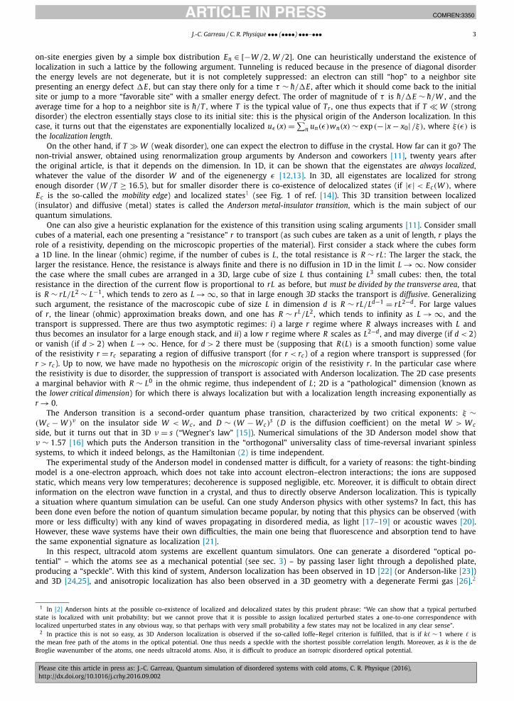
Fig. 1. Left: Tight-binding model of a perfect crystal. Energy levels associated with individual sites have identical energies. Right: Disordered “crystal”, the site energies have a random distribution.

best known of these signatures is level repulsion, implying that the energy level-spacing distribution tends to zero when spacing tends to zero [1].

Quantum disorder has been intensively investigated for almost 60 years since P.W. Anderson introduced his paradigmatic model [2], describing (in a somewhat crude, but mathematically tractable, way) the quantum physics of disordered media. The model’s main prediction is the existence of exponentially-localized eigenstates in space, in sharp contrast with the delocalized Bloch eigenstates of a prefect crystal. In three dimensions (3D), the model predicts the existence of a second-order quantum phase transition between delocalized (“metal”) and localized (“insulator”) phases, known as the Anderson metal–insulator transition, which is the main subject of the present work.

The kicked rotor is a paradigm of Hamiltonian classical and quantum chaos. The classical version of this simple system displays a wealth of dynamic behaviors, which make it well adapted for studies of quantum chaos. Surprisingly, in its quantum version, the classical chaotic diffusion in momentum space can be totally suppressed, leading to an exponential localization in momentum space, called dynamical localization [3], which strongly evokes Anderson localization. Indeed, it has been proved [4] that there exists a mathematical mapping of the kicked rotor Hamiltonian onto a 1D Anderson Hamiltonian. The kicked rotor can thus be used to quantum-simulate Anderson physics.

The original idea of quantum simulation seems to be due to Feynman [5]. Basically, the idea of a quantum simulator (in today’s sense, which is somewhat different from Feynman’s) is to realize a physical model originally introduced in a certain domain using a “simulator” from another domain, which presents practical or theoretical advantages compared to the original model. The present work describes a quantum simulator obtained by the encounter of two paradigms: the Anderson model, originally proposed in a condensed-matter context, is simulated using the atomic kicked rotor formed by laser-cooled atoms interacting with laser light. Another beautiful example of quantum simulation is the realization of Bose–(or Fermi–)Hubbard physics with ultracold atoms, e.g., the observation of the Mott transition [6]; other examples can be found in refs. [7,8].

2. The Anderson model in a nutshell

One can have a taste of the Anderson model by considering a 1D crystal in a tight-binding description [9]. Fig. 1 (left) shows schematically the tight-binding description of a crystal: the electron wave function is written in a basis of states localized in individual potential wells, usually the so-called Wannier states wn(x) ≡ 〈x |n〉 [10,9] where |n〉 is the basis ket corresponding to site n. Supposing that temperature is low enough that only the ground state of each well is in play here, the translation symmetry implies i) that the levels corresponding to each well all have the same energy E0 and ii) that wn(x) = w0(x −n). Tunneling between wells a distance r apart (in units of the lattice constant) in a Hamiltonian of the form H = p2/2m + V (x) (with V (x + n) = V (x), n ∈ Z) is thus allowed, with an amplitude T (n, n + r) = ∫

w∗n(x)H wn+r(x) dx =∫

w∗0(x)H wr(x) dx ≡ Tr , so that the Hamiltonian can be written

HTB =∑n∈Z

(E0 |n〉 〈n| +

∑r∈Z∗

Tr |n〉 〈n + r|)

(1)

The first (“diagonal”) term describes the on-site energy, and the second (“hopping”) one describes tunneling between sites a distance r apart. The equation for an eigenstate uε(x) = ∑

n un wn(x) in position representation is thus

Enun +∑r �=0

Trun+r = εun (2)

with, in the present case, En = E0.Anderson postulated [2] that the main effect of disorder in such systems is to randomize the on-site energy [Fig. 1 (right)],

the effect on the coupling coefficients Tr being “second-order”; this hypothesis is called “diagonal disorder”. Anderson used

JID:COMREN AID:3350 /SSU [m3G; v1.190; Prn:13/10/2016; 8:37] P.3 (1-16)

J.-C. Garreau / C. R. Physique ••• (••••) •••–••• 3

on-site energies given by a simple box distribution En ∈ [−W /2, W /2]. One can heuristically understand the existence of localization in such a lattice by the following argument. Tunneling is reduced because in the presence of diagonal disorder the energy levels are not degenerate, but it is not completely suppressed: an electron can still “hop” to a neighbor site presenting an energy defect �E , but can stay there only for a time τ ∼ h̄/�E , after which it should come back to the initial site or jump to a more “favorable site” with a smaller energy defect. The order of magnitude of τ is h̄/�E ∼ h̄/W , and the average time for a hop to a neighbor site is h̄/T , where T is the typical value of Tr , one thus expects that if T W (strong disorder) the electron essentially stays close to its initial site: this is the physical origin of the Anderson localization. In this case, it turns out that the eigenstates are exponentially localized uε (x) = ∑

n un(ε)wn(x) ∼ exp (−|x − x0|/ξ), where ξ(ε) is the localization length.

On the other hand, if T W (weak disorder), one can expect the electron to diffuse in the crystal. How far can it go? The non-trivial answer, obtained using renormalization group arguments by Anderson and coworkers [11], twenty years after the original article, is that it depends on the dimension. In 1D, it can be shown that the eigenstates are always localized, whatever the value of the disorder W and of the eigenenergy ε [12,13]. In 3D, all eigenstates are localized for strong enough disorder (W /T ≥ 16.5), but for smaller disorder there is co-existence of delocalized states (if |ε| < Ec(W ), where Ec is the so-called the mobility edge) and localized states1 (see Fig. 1 of ref. [14]). This 3D transition between localized (insulator) and diffusive (metal) states is called the Anderson metal-insulator transition, which is the main subject of our quantum simulations.

One can also give a heuristic explanation for the existence of this transition using scaling arguments [11]. Consider small cubes of a material, each one presenting a “resistance” r to transport (as such cubes are taken as a unit of length, r plays the role of a resistivity, depending on the microscopic properties of the material). First consider a stack where the cubes form a 1D line. In the linear (ohmic) regime, if the number of cubes is L, the total resistance is R ∼ rL: The larger the stack, the larger the resistance. Hence, the resistance is always finite and there is no diffusion in 1D in the limit L → ∞. Now consider the case where the small cubes are arranged in a 3D, large cube of size L thus containing L3 small cubes: then, the total resistance in the direction of the current flow is proportional to rL as before, but must be divided by the transverse area, that is R ∼ rL/L2 ∼ L−1, which tends to zero as L → ∞, so that in large enough 3D stacks the transport is diffusive. Generalizing such argument, the resistance of the macroscopic cube of size L in dimension d is R ∼ rL/Ld−1 = rL2−d . For large values of r, the linear (ohmic) approximation breaks down, and one has R ∼ rL/L2, which tends to infinity as L → ∞, and the transport is suppressed. There are thus two asymptotic regimes: i) a large r regime where R always increases with L and thus becomes an insulator for a large enough stack, and ii) a low r regime where R scales as L2−d , and may diverge (if d < 2) or vanish (if d > 2) when L → ∞. Hence, for d > 2 there must be (supposing that R(L) is a smooth function) some value of the resistivity r = rc separating a region of diffusive transport (for r < rc) of a region where transport is suppressed (for r > rc). Up to now, we have made no hypothesis on the microscopic origin of the resistivity r. In the particular case where the resistivity is due to disorder, the suppression of transport is associated with Anderson localization. The 2D case presents a marginal behavior with R ∼ L0 in the ohmic regime, thus independent of L; 2D is a “pathological” dimension (known as the lower critical dimension) for which there is always localization but with a localization length increasing exponentially as r → 0.

The Anderson transition is a second-order quantum phase transition, characterized by two critical exponents: ξ ∼(Wc − W )ν on the insulator side W < Wc , and D ∼ (W − Wc)

s (D is the diffusion coefficient) on the metal W > Wc

side, but it turns out that in 3D ν = s (“Wegner’s law” [15]). Numerical simulations of the 3D Anderson model show that ν ∼ 1.57 [16] which puts the Anderson transition in the “orthogonal” universality class of time-reversal invariant spinless systems, to which it indeed belongs, as the Hamiltonian (2) is time independent.

The experimental study of the Anderson model in condensed matter is difficult, for a variety of reasons: the tight-binding model is a one-electron approach, which does not take into account electron–electron interactions; the ions are supposed static, which means very low temperatures; decoherence is supposed negligible, etc. Moreover, it is difficult to obtain direct information on the electron wave function in a crystal, and thus to directly observe Anderson localization. This is typically a situation where quantum simulation can be useful. Can one study Anderson physics with other systems? In fact, this has been done even before the notion of quantum simulation became popular, by noting that this physics can be observed (with more or less difficulty) with any kind of waves propagating in disordered media, as light [17–19] or acoustic waves [20]. However, these wave systems have their own difficulties, the main one being that fluorescence and absorption tend to have the same exponential signature as localization [21].

In this respect, ultracold atom systems are excellent quantum simulators. One can generate a disordered “optical po-tential” – which the atoms see as a mechanical potential (see sec. 3) – by passing laser light through a depolished plate, producing a “speckle”. With this kind of system, Anderson localization has been observed in 1D [22] (or Anderson-like [23]) and 3D [24,25], and anisotropic localization has also been observed in a 3D geometry with a degenerate Fermi gas [26].2

1 In [2] Anderson hints at the possible co-existence of localized and delocalized states by this prudent phrase: “We can show that a typical perturbed state is localized with unit probability; but we cannot prove that it is possible to assign localized perturbed states a one-to-one correspondence with localized unperturbed states in any obvious way, so that perhaps with very small probability a few states may not be localized in any clear sense”.

2 In practice this is not so easy, as 3D Anderson localization is observed if the so-called Ioffe–Regel criterion is fulfilled, that is if k� ∼ 1 where � is the mean free path of the atoms in the optical potential. One thus needs a speckle with the shortest possible correlation length. Moreover, as k is the de Broglie wavenumber of the atoms, one needs ultracold atoms. Also, it is difficult to produce an isotropic disordered optical potential.

JID:COMREN AID:3350 /SSU [m3G; v1.190; Prn:13/10/2016; 8:37] P.4 (1-16)

4 J.-C. Garreau / C. R. Physique ••• (••••) •••–•••

These are beautiful experiments, but the determination of the mobility edge is challenging, because of the dependence of the localization length on the energy (which is hard to control inside the speckle). The critical exponent of the transition could not yet been measured with such systems.

The quantum simulator described above, obtained by placing ultracold atoms in a speckle potential, is a “direct trans-lation” of the Anderson model in cold-atom language. Are there other models that are mathematically equivalent to the Anderson model without being a direct translation? Indeed yes, the atomic kicked rotor meets these conditions, and presents considerable interest for the simulation of the Anderson transition, as we shall see in the next sections.

3. The kicked rotor and the Anderson model

3.1. The kicked rotor and the dynamical localization

In its simplest version, the kicked rotor (KR) is formed by a particle constrained to move on a circular orbit to which periodic (period T1) delta-pulses (kicks) of a constant force are applied. As only the component of the force along the orbit influences the particle’s motion, one has the Hamiltonian

Hkr = L2

2+ K cos θ

∑n∈Z

δ(t − n) (3)

where (L, θ) are conjugate variables corresponding to the angular momentum and the angular position of the particle, and we use units in which the momentum of inertia is 1, time units of the period T1 , and K cos θ is the torque applied at each kick. The corresponding Hamilton equations can be easily integrated over one period, giving a stroboscopic map for each t = n+ , known as the Standard Map:

θn+1 = θn + Ln, Ln+1 = Ln + K sin θn+1 (4)

This very simple map – easy to implement numerically – displays a wealth of dynamical behaviors going from regular (K 1), to mixed (chaos and regular orbits, 1 � K � 5) and to developed (ergodic) chaos (K > 5). In the last case, the motion is simply a diffusion in momentum space: L2 = 2Dt (the overbar denotes a classical average in phase space). This sequence of behaviors for increasing K very closely follows the Kolmogorov–Arnol’d–Moser (KAM) scenario [27]. This has made the Standard Map a paradigm for studies of classical Hamiltonian chaos.

It is straightforward to write the Schrödinger equation for the KR Hamiltonian (3). However, for periodic systems, the one-period evolution operator is often more useful:

U (1) = exp

(−i

L2

2h̄

)exp

(−i

K cos θ

h̄

)= exp

(−i

m2h̄

2

)exp

(−i

K cos θ

h̄

)(5)

where, in the second expression, we used the quantization of the angular momentum L = mh̄. Although θ and L do not commute, the presence of the delta function allows one to neglect L2/2h̄ compared to K cos θδ(0)/h̄ in the argument of the second exponential, so that U effectively factorizes into a “free evolution” and a “kick” part. One can efficiently simulate such evolution. As the kick part is diagonal in the position space and the free propagation part in the momentum space, the evolution over a period “costs” only two Fourier transforms and two multiplications. This makes the kicked rotor a privileged ground for studies of quantum chaos. The typical action integrated over one period is, in units of h̄, L2T1/h̄ ∼ m2T1, so that by adjusting T1 one controls the “quantum character” of the dynamics. More precisely, by increasing T1 one reduces the time scale for quantum effects to become dominant (the so-called Heisenberg time); one can thus think of an “effective Planck constant” h̄eff ∝ T1. In the momentum representation, the kick operator is proportional to ∑

j J j(K/h̄eff) exp (i jθ) |m + j〉 〈m| ( J j(x) is the Bessel function of first type and order j), its application thus generates “side bands” in the momentum distribution within a range K/h̄eff. After a few kicks, the amplitude for a given angular momentum mh̄ is the sum of such contributions, generating an interference that leads to purely quantum effects.

The first numerical study of the quantum kicked rotor (QKR) [3] produced a surprising result: in the ergodic regime K > 5, a classical diffusion in momentum space was observed for short times, but for later times the kinetic energy

⟨L2

⟩/2

was observed to saturate at a constant value.3 At the same time, the momentum distribution was observed to change from a Gaussian to an exponential exp (−|m|/ξ), which hints to a relation to the Anderson localization. This phenomenon was called “dynamical localization”, i.e. localization in the momentum space.

3.2. The atomic kicked rotor

Graham et al. [28] first suggested using cold atoms for observing dynamical localization, and the first experimental observation was made by Raizen and coworkers in 1994 [29], with a somewhat different system. In later experiments [30], this same group used an atomic realization of the QKR, obtained by placing laser-cooled atoms in a far-detuned standing

3 In [3] the authors write “We do not yet understand this quantum anomaly”.

JID:COMREN AID:3350 /SSU [m3G; v1.190; Prn:13/10/2016; 8:37] P.5 (1-16)

J.-C. Garreau / C. R. Physique ••• (••••) •••–••• 5

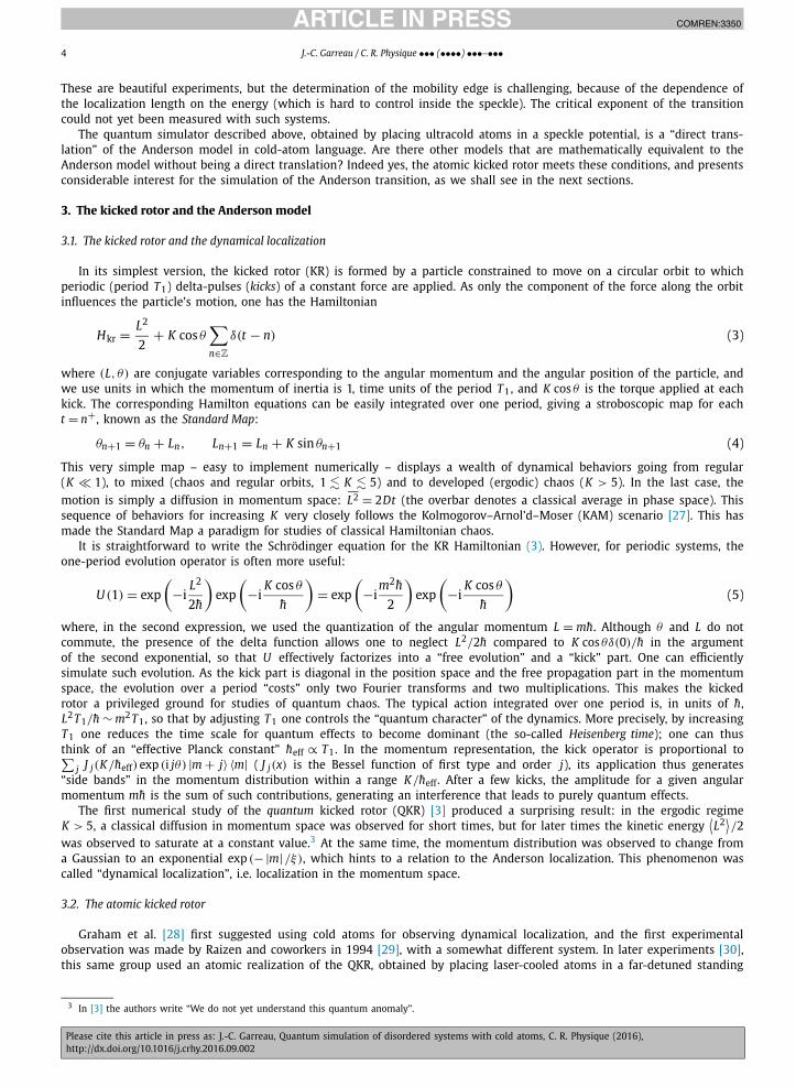
Fig. 2. Experimental setup. Top: Schematic view. An acousto-optical modulator (AOM) is driven by a pulsed radio-frequency (RF) signal. If the RF is on (pulses), the AOM deflects the laser beam, which is reflected backwards by a mirror and generates a standing wave that interacts with the atomic cloud. If the RF driving is off, the undeflected beam does not interact with the atoms. Bottom: “Less schematic” view of the experiment.

wave. In such conditions, the atoms see the radiation as a sinusoidal mechanical potential – called an optical or dipole potential – affecting their center of mass motion. If the radiation is periodically pulsed (T1 ∼ 30 μs4) with very short pulses,5 then the corresponding Hamiltonian is

Hakr = p2

2μ+ K cos x

∑n

δ(t − n) (6)

which has the same form as (3). Distances are measured in units of λL/4π , where λL = 2π/kL is the laser wavelength, time in units of the pulse period T1, and K ∝ T1 I/�, where I ∼ 10 W/cm2 is the radiation intensity and � ∼ ±20 GHz ≈3 × 103� (� is the natural width of the transition) its detuning with respect to the atomic transition. The reduced Planck constant is in this case heff ≡ k- = 4h̄k2

L T1/M ∼ 2.9, where M is the mass of the atom. By convention, we shall use sans serif characters to indicate dimensioned quantities, e.g., x = 2kLx, t = t/T1, etc. It is useful to chose units such that μ = k-−2

in (6), so that p = p/2h̄kL . The lattice constant is λL/2, comparable to the de Broglie wavelength of laser-cooled atoms ∼ λL/3, ensuring the quantum character of the dynamics. The laser-atom detuning must be large enough that the typical spontaneous emission time ∼ (

� I/�2)−1

is larger than the duration of the experiment, otherwise the random character of the phase changes induced by the spontaneous emission process produces lethal decoherence effects [31,32]. Because the momentum exchanges between the standing wave and the atom are directed along kL , the dynamics is effectively 1D, the transverse directions, not being affected by the radiation, evolve independently of the longitudinal direction.

Our basic experimental setup is shown schematically in Fig. 2 (top): cesium atoms are laser-cooled in a magneto-optical trap to temperatures ∼ 2 μK. The (dissipative) trap is then turned off, and pulses of a far-detuned standing wave applied to the atoms (in such conditions, the resulting dynamics is quantum). The final momentum distribution of the atoms can be measured by a variety of techniques. In a first version of the experiment, the standing wave was horizontal, to avoid gravi-tation acceleration, but this limited the interaction time of the freely-falling atoms with the standing wave. In more recent times, we used a vertical standing wave formed by two frequency-chirped laser beams to compensate gravity: by shifting the frequency of one beam with respect to the other, we obtain a standing wave whose nodes are accelerated in the vertical direction. By adjusting this acceleration so that it equals the gravity acceleration, a kicked rotor is obtained in the free-fallingreference frame [33]. For measuring the momentum distribution of the atoms, our group used for many years stimulated Raman transitions between hyperfine sublevels [34,35], as we changed to the vertical standing wave configuration, we could use a standard time-of-flight technique.

4 We indicate typical values used in our setup for the parameters.5 The typical time scale of the atom dynamics should be much larger than the pulse duration, in practice this means pulses of a few hundred ns.

JID:COMREN AID:3350 /SSU [m3G; v1.190; Prn:13/10/2016; 8:37] P.6 (1-16)

6 J.-C. Garreau / C. R. Physique ••• (••••) •••–•••

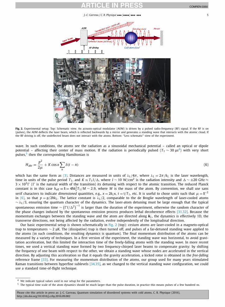
Fig. 3. Experimental observation of dynamical localization: Exponentially-localized momentum distribution (p) recorded at t = 30 kicks. The left plot in linear scale shows a fit by an exponential shape (blue curve). The right plot in semilog scale confirms the exponential localization. Parameters are K = 7.2, k- = 2.89.

Because of the spatial periodicity of the optical potential, quasimomentum is a constant of motion. Hence kicks couple only momentum components separated by 2h̄kL , so that starting with a well-defined momentum p0 leads to a discrete momentum distribution at values (m +β)2h̄kL with m ∈ Z and β the fractional part of p0. The main difference between this “unfolded” kicked rotor and the “standard” version described by the Hamiltonian (3) is the existence of quasimomentum families. One can show (see sec. 3.3) that each quasimomentum family maps to a particular Anderson eigenvector with a given disorder.6 This is quite useful in many situations, as averaging over quasimomentum (that is, starting with an initial state that has a width comparable to the Brillouin zone width 2h̄kL ) is equivalent to average over disorder in the corre-sponding Anderson model. In other situations, however, this averaging can hide interesting effects. Typically, the momentum distribution of cold atoms (that is, of atoms cooled in a magneto-optical trap) populate a few Brillouin zones, but that of ultracold atoms (e.g., a Bose–Einstein condensate) can be only a small fraction of the Brillouin zone. In general, interatomic interactions are negligible, if not from the start, after a few kicks, as the spatial density dilutes very quickly due to the diffusion in the momentum space. An experimentally observed momentum distribution is shown in Fig. 3.

3.3. Equivalence between dynamical localization and the 1D Anderson localization

The observation that the momentum distribution takes an exponential shape in dynamical localization strongly evokes Anderson localization. A few years after the discovery of dynamical localization, Fishman, Grempel and Prange established a mathematical equivalence between the two [36,4]. This equivalence is basically a matter of algebra, but as it is the ground for our using of the KR as a quantum simulator of Anderson physics, it is useful to see how it arises.

As the KR is periodic in time, the Floquet operator technique can be used, which consists in diagonalizing the one-period evolution operator (5):

exp

(−i

p2

2k-

)exp

(−i

K cos x

k-

)|ω〉 = e−iω |ω〉 (7)

where |ω〉 is the Floquet “quasi-eigenstate”, and ω ∈ [0, 2π) is the corresponding “quasi-energy”. The “stroboscopic” evolu-tion of any initial state |ψ0〉 at integer times t = n is then simply:

|ψn〉 =∑ω

e−iωn 〈ω |ψ0〉 |ω〉 (8)

Using this expansion, one can write⟨p2

⟩=

∑ω

|〈ω |ψ0〉|2 〈ω| p2 |ω〉 +∑ω �=ω′

〈ψ0∣∣ω′⟩ 〈ω |ψ0〉ei

(ω′−ω

)n ⟨

ω′∣∣ p2 |ω〉 (9)

If the Floquet spectrum is dense (which happens if the system is in the quantum-chaotic regime) and n = t/T1 is large enough that

(ω′ − ω

)n ≥ π/2, the contributions in the second term tend to interfere destructively, and only the first sum

ω′ = ω survives:⟨p2

⟩→ p2∞ =

∑ω

|〈ω |ψ0〉|2 〈ω| p2 |ω〉 (t > tloc) (10)

after some localization time tloc. The kinetic energy thus tends to saturate for t > tloc, as observed numerically by Casati et al. [3].

6 Taking quasimomentum into account, Eq. (14) becomes En = tan(ω/2 − (m + β)2k-/4

).

JID:COMREN AID:3350 /SSU [m3G; v1.190; Prn:13/10/2016; 8:37] P.7 (1-16)

J.-C. Garreau / C. R. Physique ••• (••••) •••–••• 7

As dynamical localization manifests itself in momentum space, it is natural to express the Floquet states in the momen-tum basis. However, the kick operator is not diagonal in this representation, so Fishman, Grempel, and Prange used the trigonometric identity

eix = 1 + i tan(x/2)

1 − i tan(x/2)(11)

to transform equation (7) into

1 + i tan v̂

1 − i tan v̂

(1 − i tan t̂

) 1

1 + i tan t̂|ω〉 = |ω〉 (12)

with v̂ = ω/2 − p̂2/4h̄ and t̂ = κ cos x̂/2 (κ := K/k-). Decomposing (1 + i tan t̂

)−1 |ω〉 = ∑s us |s〉 on the basis momentum

eigenstates |s〉 gives |ω〉 = (1 + i tan t̂

)∑s us |s〉. Projecting (12) on a momentum eigenstate 〈m| and using the previous

identity leads, after some (cumbersome) algebra, to

tan (vm) um +∑r �=0

trum+r = −t0um (13)

where vm = ω/2 − m2k-/4 and tr = − 〈m| tan t̂ |m + r〉, which has the form of the 1D tight-binding equation (2) with the equivalences

En ↔ tan vm = tan

(ω

2− m2k-

4

)(14)

Tr ↔ tr = 1

2π

2π∫0

dxeirx tan (κ cos x/2) (15)

Note that the kick term in the evolution operator basically maps on the hopping coefficient tr ∼ K/k- that controls the transport, while the free propagation term maps on the equivalent of the diagonal disorder, tan vm , which is essentially controlled by k-. Hence the Anderson control parameter T /W translates into K/k- to within a numerical factor.

There are however differences with respect to the Anderson model:1) in (13), all eigenstates um correspond to the same Anderson eigenvalue ε = −t0 (according to (15), by symmetry,

t0 = 0). This in particular means that all localized states for the KR have the same localization length ξ , in contrast to the 1D Anderson eigenstates, whose localization length scales as (T /W )2 and depend on the energy [12,13]. This fact has an important consequence: if, in (10), the width of the initial state ψ0(p) (supposed centered at p = 0) is much smaller than ξ , this state will be projected only over Floquet eigenstates spreading over a range ∼ ξ ; one thus concludes that p2∞ ≈ p2

loc ∼ ξ2 = cte, i.e. the asymptotic value of the kinetic energy does not depend on the initial state.7

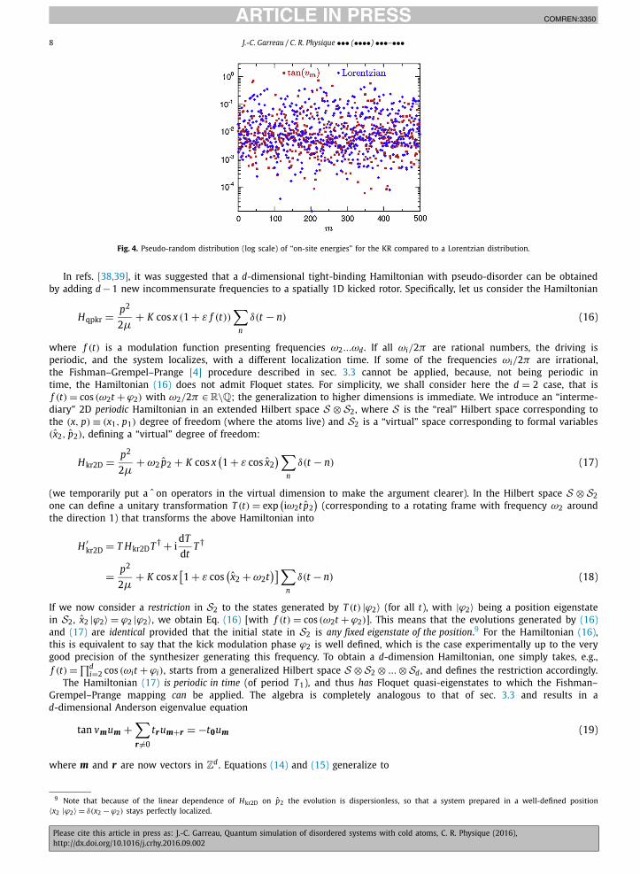
2) The Anderson model random on-site energies map into the deterministic function tan vm . However, for large enough values of k- ∝ T1, this functions varies strongly (Fig. 4), at the condition that k- is an irrational number; otherwise the function is periodic in m.8

3) The localized states |u〉 = ∑m um |m〉 = (

1 + i tan t̂)−1 |ω〉 are not the Floquet states, indeed |ω〉 = 2eit

(eit̂ + e−it̂

)|u〉.

As t̂ is “half” the kick operator, the Floquet state is, to within a phase factor, a superposition of the localized state advanced and retard of half a kick; it has thus essentially the same localization properties.

The 1D Anderson localization length for fixed energy is proportional to (T /W )2 [12,13] and the fact that the dynamics is diffusive for t < tloc with an early-time (classical) diffusion constant D ≈ K 2/4, so that p2

loc ∼ 2Dtloc, imply that both tloc

and ploc are proportional to (K/k-)2.

3.4. The quasiperiodic kicked rotor and its equivalence to a 3D Anderson model

In order to study the Anderson transition, one needs an analog of the 3D Anderson model. A simple idea would be to use a 3D kicked rotor, by kicking a 3D optical lattice [37]. This is experimentally complicated for several reasons, the main ones being the fact that gravity breaks the symmetry among directions and the delicate control of the phase relations of the various beams forming a separable 3D optical lattice.

7 Moreover, the QKR does not map onto a nearest-neighbor Anderson model. The nearest-neighbor approximation is usual in the Anderson model context, but it is not necessary: it suffices that the hopping coefficients tr decreases fast enough (at least as r−3) to ensure the convergence of the perturbation series used by Anderson (see [2]).

8 If k- is rational, a totally different – but also interesting – behavior arises, called “quantum resonance”, namely a ballistic increase in the kinetic energy ⟨p2

⟩ ∝ t2 (for rational values of the quasimomentum β).

JID:COMREN AID:3350 /SSU [m3G; v1.190; Prn:13/10/2016; 8:37] P.8 (1-16)

8 J.-C. Garreau / C. R. Physique ••• (••••) •••–•••

Fig. 4. Pseudo-random distribution (log scale) of “on-site energies” for the KR compared to a Lorentzian distribution.

In refs. [38,39], it was suggested that a d-dimensional tight-binding Hamiltonian with pseudo-disorder can be obtained by adding d − 1 new incommensurate frequencies to a spatially 1D kicked rotor. Specifically, let us consider the Hamiltonian

Hqpkr = p2

2μ+ K cos x (1 + ε f (t))

∑n

δ(t − n) (16)

where f (t) is a modulation function presenting frequencies ω2...ωd . If all ωi/2π are rational numbers, the driving is periodic, and the system localizes, with a different localization time. If some of the frequencies ωi/2π are irrational, the Fishman–Grempel–Prange [4] procedure described in sec. 3.3 cannot be applied, because, not being periodic in time, the Hamiltonian (16) does not admit Floquet states. For simplicity, we shall consider here the d = 2 case, that is f (t) = cos (ω2t + ϕ2) with ω2/2π ∈ R\Q; the generalization to higher dimensions is immediate. We introduce an “interme-diary” 2D periodic Hamiltonian in an extended Hilbert space S ⊗ S2, where S is the “real” Hilbert space corresponding to the (x, p) ≡ (x1, p1) degree of freedom (where the atoms live) and S2 is a “virtual” space corresponding to formal variables (x̂2, p̂2), defining a “virtual” degree of freedom:

Hkr2D = p2

2μ+ ω2 p̂2 + K cos x

(1 + ε cos x̂2

)∑n

δ(t − n) (17)

(we temporarily put a ̂ on operators in the virtual dimension to make the argument clearer). In the Hilbert space S ⊗ S2one can define a unitary transformation T (t) = exp

(iω2t p̂2

)(corresponding to a rotating frame with frequency ω2 around

the direction 1) that transforms the above Hamiltonian into

H ′kr2D = T Hkr2DT † + i

dT

dtT †

= p2

2μ+ K cos x

[1 + ε cos

(x̂2 + ω2t

)]∑n

δ(t − n) (18)

If we now consider a restriction in S2 to the states generated by T (t) |ϕ2〉 (for all t), with |ϕ2〉 being a position eigenstate in S2, x̂2 |ϕ2〉 = ϕ2 |ϕ2〉, we obtain Eq. (16) [with f (t) = cos (ω2t + ϕ2)]. This means that the evolutions generated by (16)and (17) are identical provided that the initial state in S2 is any fixed eigenstate of the position.9 For the Hamiltonian (16), this is equivalent to say that the kick modulation phase ϕ2 is well defined, which is the case experimentally up to the very good precision of the synthesizer generating this frequency. To obtain a d-dimension Hamiltonian, one simply takes, e.g., f (t) = ∏d

i=2 cos (ωit + ϕi), starts from a generalized Hilbert space S ⊗ S2 ⊗ ... ⊗ Sd , and defines the restriction accordingly.The Hamiltonian (17) is periodic in time (of period T1), and thus has Floquet quasi-eigenstates to which the Fishman–

Grempel–Prange mapping can be applied. The algebra is completely analogous to that of sec. 3.3 and results in a d-dimensional Anderson eigenvalue equation

tan vmum +∑r �=0

trum+r = −t0um (19)

where m and r are now vectors in Zd . Equations (14) and (15) generalize to

9 Note that because of the linear dependence of Hkr2D on p̂2 the evolution is dispersionless, so that a system prepared in a well-defined position 〈x2 |ϕ2〉 = δ(x2 − ϕ2) stays perfectly localized.

JID:COMREN AID:3350 /SSU [m3G; v1.190; Prn:13/10/2016; 8:37] P.9 (1-16)

J.-C. Garreau / C. R. Physique ••• (••••) •••–••• 9

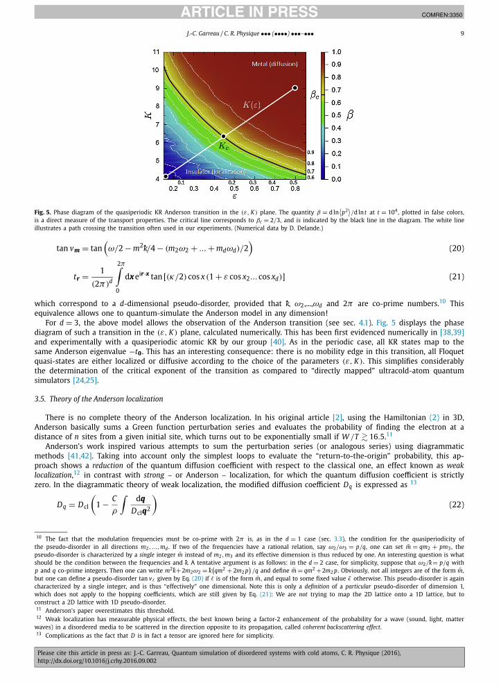
Fig. 5. Phase diagram of the quasiperiodic KR Anderson transition in the (ε, K ) plane. The quantity β = d ln ⟨p2

⟩/d ln t at t = 104, plotted in false colors,

is a direct measure of the transport properties. The critical line corresponds to βc = 2/3, and is indicated by the black line in the diagram. The white line illustrates a path crossing the transition often used in our experiments. (Numerical data by D. Delande.)

tan vm = tan(ω/2 − m2k-/4 − (m2ω2 + ... + mdωd)/2

)(20)

tr = 1

(2π)d

2π∫0

dx eir·x tan [(κ/2) cos x (1 + ε cos x2... cos xd)] (21)

which correspond to a d-dimensional pseudo-disorder, provided that k-, ω2,...,ωd and 2π are co-prime numbers.10 This equivalence allows one to quantum-simulate the Anderson model in any dimension!

For d = 3, the above model allows the observation of the Anderson transition (see sec. 4.1). Fig. 5 displays the phase diagram of such a transition in the (ε, K ) plane, calculated numerically. This has been first evidenced numerically in [38,39]and experimentally with a quasiperiodic atomic KR by our group [40]. As in the periodic case, all KR states map to the same Anderson eigenvalue −t0 . This has an interesting consequence: there is no mobility edge in this transition, all Floquet quasi-states are either localized or diffusive according to the choice of the parameters (ε, K ). This simplifies considerably the determination of the critical exponent of the transition as compared to “directly mapped” ultracold-atom quantum simulators [24,25].

3.5. Theory of the Anderson localization

There is no complete theory of the Anderson localization. In his original article [2], using the Hamiltonian (2) in 3D, Anderson basically sums a Green function perturbation series and evaluates the probability of finding the electron at a distance of n sites from a given initial site, which turns out to be exponentially small if W /T � 16.5.11

Anderson’s work inspired various attempts to sum the perturbation series (or analogous series) using diagrammatic methods [41,42]. Taking into account only the simplest loops to evaluate the “return-to-the-origin” probability, this ap-proach shows a reduction of the quantum diffusion coefficient with respect to the classical one, an effect known as weak localization,12 in contrast with strong – or Anderson – localization, for which the quantum diffusion coefficient is strictly zero. In the diagrammatic theory of weak localization, the modified diffusion coefficient Dq is expressed as 13

Dq = Dcl

(1 − C

ρ

∫dq

Dclq2

)(22)

10 The fact that the modulation frequencies must be co-prime with 2π is, as in the d = 1 case (sec. 3.3), the condition for the quasiperiodicity of the pseudo-disorder in all directions m2, ..., md . If two of the frequencies have a rational relation, say ω2/ω3 = p/q, one can set m̄ = qm2 + pm3, the pseudo-disorder is characterized by a single integer m̄ instead of m2, m3 and its effective dimension is thus reduced by one. An interesting question is what should be the condition between the frequencies and k-. A tentative argument is as follows: in the d = 2 case, for simplicity, suppose that ω2/k- = p/q with p and q co-prime integers. Then one can write m2k-+2m2ω2 = k-

(qm2 + 2m2 p

)/q and define m̄ = qm2 +2m2 p. Obviously, not all integers are of the form m̄,

but one can define a pseudo-disorder tan v� given by Eq. (20) if � is of the form m̄, and equal to some fixed value ε̄ otherwise. This pseudo-disorder is again characterized by a single integer, and is thus “effectively” one dimensional. Note this is only a definition of a particular pseudo-disorder of dimension 1, which does not apply to the hopping coefficients, which are still given by Eq. (21): We are not trying to map the 2D lattice onto a 1D lattice, but to construct a 2D lattice with 1D pseudo-disorder.11 Anderson’s paper overestimates this threshold.12 Weak localization has measurable physical effects, the best known being a factor-2 enhancement of the probability for a wave (sound, light, matter

waves) in a disordered media to be scattered in the direction opposite to its propagation, called coherent backscattering effect.13 Complications as the fact that D is in fact a tensor are ignored here for simplicity.

JID:COMREN AID:3350 /SSU [m3G; v1.190; Prn:13/10/2016; 8:37] P.10 (1-16)

10 J.-C. Garreau / C. R. Physique ••• (••••) •••–•••

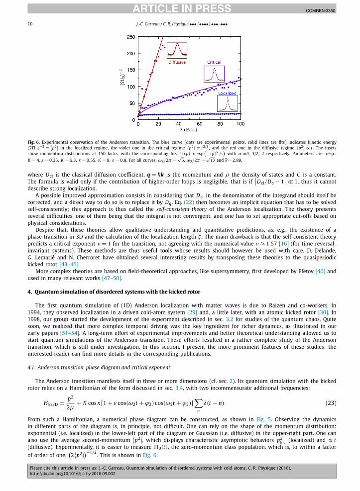
Fig. 6. Experimental observation of the Anderson transition. The blue curve (dots are experimental points, solid lines are fits) indicates kinetic energy (2 0)−2 ∝ ⟨

p2⟩

in the localized regime, the violet one in the critical regime 〈p2〉 ∝ t2/3, and the red one in the diffusive regime 〈p2〉 ∝ t . The insets show momentum distributions at 150 kicks, with the corresponding fits, (p) ∝ exp

(−|p|α /s)

with α =1, 3/2, 2 respectively. Parameters are, resp.: K = 4, ε = 0.35, K = 6.3, ε = 0.55, K = 9, ε = 0.8. For all curves, ω2/2π = √

5, ω3/2π = √13 and k- = 2.89.

where Dcl is the classical diffusion coefficient, q = h̄k is the momentum and ρ the density of states and C is a constant. The formula is valid only if the contribution of higher-order loops is negligible, that is if

∣∣Dcl/Dq − 1∣∣ 1, thus it cannot

describe strong localization.A possible improved approximation consists in considering that Dcl in the denominator of the integrand should itself be

corrected, and a direct way to do so is to replace it by Dq . Eq. (22) then becomes an implicit equation that has to be solved self-consistently; this approach is thus called the self-consistent theory of the Anderson localization. The theory presents several difficulties, one of them being that the integral is not convergent, and one has to set appropriate cut-offs based on physical considerations.

Despite that, these theories allow qualitative understanding and quantitative predictions, as, e.g., the existence of a phase transition in 3D and the calculation of the localization length ξ . The main drawback is that the self-consistent theory predicts a critical exponent ν = 1 for the transition, not agreeing with the numerical value ν ≈ 1.57 [16] (for time-reversal-invariant systems). These methods are thus useful tools whose results should however be used with care. D. Delande, G. Lemarié and N. Cherroret have obtained several interesting results by transposing these theories to the quasiperiodic kicked rotor [43–45].

More complex theories are based on field-theoretical approaches, like supersymmetry, first developed by Efetov [46] and used in many relevant works [47–50].

4. Quantum simulation of disordered systems with the kicked rotor

The first quantum simulation of (1D) Anderson localization with matter waves is due to Raizen and co-workers. In 1994, they observed localization in a driven cold-atom system [29] and, a little later, with an atomic kicked rotor [30]. In 1998, our group started the development of the experiment described in sec. 3.2 for studies of the quantum chaos. Quite soon, we realized that more complex temporal driving was the key ingredient for richer dynamics, as illustrated in our early papers [51–54]. A long-term effort of experimental improvements and better theoretical understanding allowed us to start quantum simulations of the Anderson transition. These efforts resulted in a rather complete study of the Anderson transition, which is still under investigation. In this section, I present the more prominent features of these studies; the interested reader can find more details in the corresponding publications.

4.1. Anderson transition, phase diagram and critical exponent

The Anderson transition manifests itself in three or more dimensions (cf. sec. 2). Its quantum simulation with the kicked rotor relies on a Hamiltonian of the form discussed in sec. 3.4, with two incommensurate additional frequencies:

Hkr3D = p2

2μ+ K cos x [1 + ε cos(ω2t + ϕ2) cos(ω3t + ϕ3)]

∑n

δ(t − n) (23)

From such a Hamiltonian, a numerical phase diagram can be constructed, as shown in Fig. 5. Observing the dynamics in different parts of the diagram is, in principle, not difficult. One can rely on the shape of the momentum distribution: exponential (i.e. localized) in the lower-left part of the diagram or Gaussian (i.e. diffusive) in the upper-right part. One can also use the average second-momentum

⟨p2

⟩, which displays characteristic asymptotic behaviors p2

loc (localized) and ∝ t(diffusive). Experimentally, it is easier to measure 0(t), the zero-momentum class population, which is, to within a factor of order of one,

(2⟨p2

⟩)−1/2. This is shown in Fig. 6.

JID:COMREN AID:3350 /SSU [m3G; v1.190; Prn:13/10/2016; 8:37] P.11 (1-16)

J.-C. Garreau / C. R. Physique ••• (••••) •••–••• 11

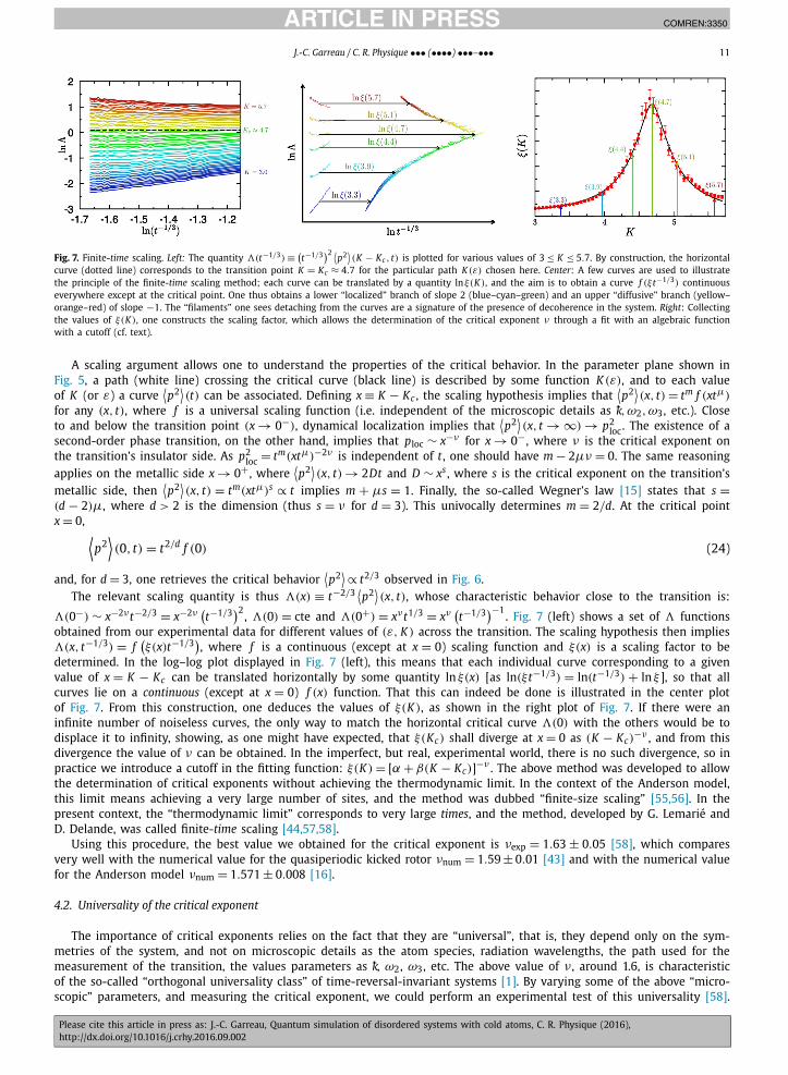
Fig. 7. Finite-time scaling. Left: The quantity �(t−1/3) ≡ (t−1/3

)2 ⟨p2

⟩(K − Kc , t) is plotted for various values of 3 ≤ K ≤ 5.7. By construction, the horizontal

curve (dotted line) corresponds to the transition point K = Kc ≈ 4.7 for the particular path K (ε) chosen here. Center: A few curves are used to illustrate the principle of the finite-time scaling method; each curve can be translated by a quantity lnξ(K ), and the aim is to obtain a curve f (ξt−1/3) continuous everywhere except at the critical point. One thus obtains a lower “localized” branch of slope 2 (blue–cyan–green) and an upper “diffusive” branch (yellow–orange–red) of slope −1. The “filaments” one sees detaching from the curves are a signature of the presence of decoherence in the system. Right: Collecting the values of ξ(K ), one constructs the scaling factor, which allows the determination of the critical exponent ν through a fit with an algebraic function with a cutoff (cf. text).

A scaling argument allows one to understand the properties of the critical behavior. In the parameter plane shown in Fig. 5, a path (white line) crossing the critical curve (black line) is described by some function K (ε), and to each value of K (or ε) a curve

⟨p2

⟩(t) can be associated. Defining x ≡ K − Kc , the scaling hypothesis implies that

⟨p2

⟩(x, t) = tm f (xtμ)

for any (x, t), where f is a universal scaling function (i.e. independent of the microscopic details as k-, ω2, ω3, etc.). Close to and below the transition point (x → 0−), dynamical localization implies that

⟨p2

⟩(x, t → ∞) → p2

loc. The existence of a second-order phase transition, on the other hand, implies that ploc ∼ x−ν for x → 0− , where ν is the critical exponent on the transition’s insulator side. As p2

loc = tm(xtμ)−2ν is independent of t , one should have m − 2μν = 0. The same reasoning applies on the metallic side x → 0+ , where

⟨p2

⟩(x, t) → 2Dt and D ∼ xs , where s is the critical exponent on the transition’s

metallic side, then ⟨p2

⟩(x, t) = tm(xtμ)s ∝ t implies m + μs = 1. Finally, the so-called Wegner’s law [15] states that s =

(d − 2)μ, where d > 2 is the dimension (thus s = ν for d = 3). This univocally determines m = 2/d. At the critical point x = 0, ⟨

p2⟩(0, t) = t2/d f (0) (24)

and, for d = 3, one retrieves the critical behavior ⟨p2

⟩ ∝ t2/3 observed in Fig. 6.The relevant scaling quantity is thus �(x) ≡ t−2/3

⟨p2

⟩(x, t), whose characteristic behavior close to the transition is:

�(0−) ∼ x−2νt−2/3 = x−2ν(t−1/3

)2, �(0) = cte and �(0+) = xνt1/3 = xν

(t−1/3

)−1. Fig. 7 (left) shows a set of � functions

obtained from our experimental data for different values of (ε, K ) across the transition. The scaling hypothesis then implies �(x, t−1/3) = f

(ξ(x)t−1/3

), where f is a continuous (except at x = 0) scaling function and ξ(x) is a scaling factor to be

determined. In the log–log plot displayed in Fig. 7 (left), this means that each individual curve corresponding to a given value of x = K − Kc can be translated horizontally by some quantity ln ξ(x) [as ln(ξt−1/3) = ln(t−1/3) + ln ξ ], so that all curves lie on a continuous (except at x = 0) f (x) function. That this can indeed be done is illustrated in the center plot of Fig. 7. From this construction, one deduces the values of ξ(K ), as shown in the right plot of Fig. 7. If there were an infinite number of noiseless curves, the only way to match the horizontal critical curve �(0) with the others would be to displace it to infinity, showing, as one might have expected, that ξ(Kc) shall diverge at x = 0 as (K − Kc)

−ν , and from this divergence the value of ν can be obtained. In the imperfect, but real, experimental world, there is no such divergence, so in practice we introduce a cutoff in the fitting function: ξ(K ) = [α + β(K − Kc)]−ν . The above method was developed to allow the determination of critical exponents without achieving the thermodynamic limit. In the context of the Anderson model, this limit means achieving a very large number of sites, and the method was dubbed “finite-size scaling” [55,56]. In the present context, the “thermodynamic limit” corresponds to very large times, and the method, developed by G. Lemarié and D. Delande, was called finite-time scaling [44,57,58].

Using this procedure, the best value we obtained for the critical exponent is νexp = 1.63 ± 0.05 [58], which compares very well with the numerical value for the quasiperiodic kicked rotor νnum = 1.59 ± 0.01 [43] and with the numerical value for the Anderson model νnum = 1.571 ± 0.008 [16].

4.2. Universality of the critical exponent

The importance of critical exponents relies on the fact that they are “universal”, that is, they depend only on the sym-metries of the system, and not on microscopic details as the atom species, radiation wavelengths, the path used for the measurement of the transition, the values parameters as k-, ω2, ω3, etc. The above value of ν , around 1.6, is characteristic of the so-called “orthogonal universality class” of time-reversal-invariant systems [1]. By varying some of the above “micro-scopic” parameters, and measuring the critical exponent, we could perform an experimental test of this universality [58].

JID:COMREN AID:3350 /SSU [m3G; v1.190; Prn:13/10/2016; 8:37] P.12 (1-16)

12 J.-C. Garreau / C. R. Physique ••• (••••) •••–•••

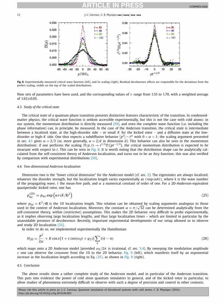
Fig. 8. Experimentally measured critical wave function (left), and its scaling (right). Residual decoherence effects are responsible for the deviations from the perfect scaling, visible on the top of the scaled distributions.

Nine sets of parameters have been used, and the corresponding values of ν range from 1.55 to 1.70, with a weighted average of 1.63±0.05.

4.3. Study of the critical state

The critical state of a quantum phase transition presents distinctive features characteristic of the transition. In condensed-matter physics, the critical wave function is seldom accessible experimentally, but this is not the case with cold atoms: in our system, the momentum distribution is directly measured [59], and even the complete wave function (i.e. including the phase information) can, in principle, be measured. In the case of the Anderson transition, the critical state is intermediate between a localized state, at the high-disorder side – or small K for the kicked rotor – and a diffusive state at the low-disorder or high-K side. One thus expects a subdiffusive behavior

⟨p2

⟩ ∼ tα with 0 < α < 1; the scaling argument presented in sec. 4.1 gives α = 2/3 (or, more generally, α = 2/d in dimension d). This behavior can also be seen in the momentum distributions: if one performs the scaling (p, t) → t1/3

(pt−1/3

), the critical momentum distribution is expected to be

invariant with respect to t . This can be seen in Fig. 8. It is worth noting that the distribution shape can be analytically cal-culated from the self-consistent theory of Anderson localization, and turns out to be an Airy function; this was also verified by comparison with experimental distributions [59].

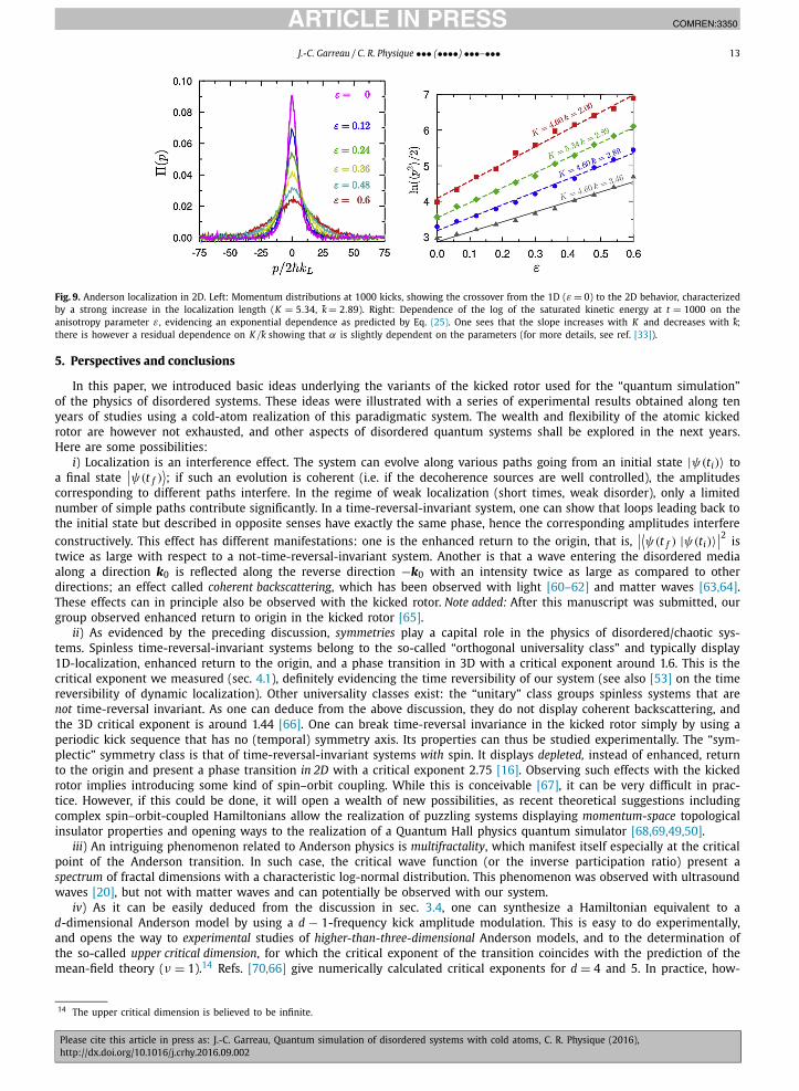
4.4. Two-dimensional Anderson localization

Dimension two is the “lower critical dimension” for the Anderson model (cf. sec. 2). The eigenstates are always localized, whatever the disorder strength, but the localization length varies exponentially as � exp (αk�), where k is the wave number of the propagating wave, � the mean-free path, and α a numerical constant of order of one. For a 2D-Anderson-equivalent quasiperiodic kicked rotor, one has

p(2D)

loc = ploc exp(αε(K/k-)2

)(25)

where ploc = K 2/4k- is the 1D localization length. This relation can be obtained by scaling arguments analogous to those used in the context of Anderson localization. Moreover, the constant α = π/

√32 can be determined analytically from the

self-consistent theory, within (restrictive) assumptions. This makes the 2D behavior very difficult to probe experimentally, as it implies observing large localization lengths, and thus large localization times – which are limited in particular by the unavoidable presence of decoherence. Recently, important experimental developments of our setup allowed us to observe and study 2D localization [33].

In order to do so, we implemented experimentally the Hamiltonian

H2D = p2

2μ+ K cos x [1 + ε cos(ω2t + ϕ2)]

∑n

δ(t − n) (26)

which maps onto a 2D Anderson model (provided ω2/2π is irrational, cf. sec. 3.4). By sweeping the modulation amplitude ε one can observe the crossover from the 1D to the 2D behavior, Fig. 9 (left), which manifests itself by an exponential increase in the localization length according to Eq. (25), as shown in Fig. 9 (right).

4.5. Conclusion

The above results show a rather complete study of the Anderson model, and in particular of the Anderson transition. This puts into evidence the power of cold atom quantum simulators in general, and of the kicked rotor in particular, to allow studies of phenomena extremely difficult to observe with such a degree of precision and control in other contexts.

JID:COMREN AID:3350 /SSU [m3G; v1.190; Prn:13/10/2016; 8:37] P.13 (1-16)

J.-C. Garreau / C. R. Physique ••• (••••) •••–••• 13

Fig. 9. Anderson localization in 2D. Left: Momentum distributions at 1000 kicks, showing the crossover from the 1D (ε = 0) to the 2D behavior, characterized by a strong increase in the localization length (K = 5.34, k- = 2.89). Right: Dependence of the log of the saturated kinetic energy at t = 1000 on the anisotropy parameter ε, evidencing an exponential dependence as predicted by Eq. (25). One sees that the slope increases with K and decreases with k-; there is however a residual dependence on K/k- showing that α is slightly dependent on the parameters (for more details, see ref. [33]).

5. Perspectives and conclusions

In this paper, we introduced basic ideas underlying the variants of the kicked rotor used for the “quantum simulation” of the physics of disordered systems. These ideas were illustrated with a series of experimental results obtained along ten years of studies using a cold-atom realization of this paradigmatic system. The wealth and flexibility of the atomic kicked rotor are however not exhausted, and other aspects of disordered quantum systems shall be explored in the next years. Here are some possibilities:

i) Localization is an interference effect. The system can evolve along various paths going from an initial state |ψ(ti)〉 to a final state

∣∣ψ(t f )⟩; if such an evolution is coherent (i.e. if the decoherence sources are well controlled), the amplitudes

corresponding to different paths interfere. In the regime of weak localization (short times, weak disorder), only a limited number of simple paths contribute significantly. In a time-reversal-invariant system, one can show that loops leading back to the initial state but described in opposite senses have exactly the same phase, hence the corresponding amplitudes interfere constructively. This effect has different manifestations: one is the enhanced return to the origin, that is,

∣∣⟨ψ(t f ) |ψ(ti)〉∣∣2 is

twice as large with respect to a not-time-reversal-invariant system. Another is that a wave entering the disordered media along a direction k0 is reflected along the reverse direction −k0 with an intensity twice as large as compared to other directions; an effect called coherent backscattering, which has been observed with light [60–62] and matter waves [63,64]. These effects can in principle also be observed with the kicked rotor. Note added: After this manuscript was submitted, our group observed enhanced return to origin in the kicked rotor [65].

ii) As evidenced by the preceding discussion, symmetries play a capital role in the physics of disordered/chaotic sys-tems. Spinless time-reversal-invariant systems belong to the so-called “orthogonal universality class” and typically display 1D-localization, enhanced return to the origin, and a phase transition in 3D with a critical exponent around 1.6. This is the critical exponent we measured (sec. 4.1), definitely evidencing the time reversibility of our system (see also [53] on the time reversibility of dynamic localization). Other universality classes exist: the “unitary” class groups spinless systems that are not time-reversal invariant. As one can deduce from the above discussion, they do not display coherent backscattering, and the 3D critical exponent is around 1.44 [66]. One can break time-reversal invariance in the kicked rotor simply by using a periodic kick sequence that has no (temporal) symmetry axis. Its properties can thus be studied experimentally. The “sym-plectic” symmetry class is that of time-reversal-invariant systems with spin. It displays depleted, instead of enhanced, return to the origin and present a phase transition in 2D with a critical exponent 2.75 [16]. Observing such effects with the kicked rotor implies introducing some kind of spin–orbit coupling. While this is conceivable [67], it can be very difficult in prac-tice. However, if this could be done, it will open a wealth of new possibilities, as recent theoretical suggestions including complex spin–orbit-coupled Hamiltonians allow the realization of puzzling systems displaying momentum-space topological insulator properties and opening ways to the realization of a Quantum Hall physics quantum simulator [68,69,49,50].

iii) An intriguing phenomenon related to Anderson physics is multifractality, which manifest itself especially at the critical point of the Anderson transition. In such case, the critical wave function (or the inverse participation ratio) present a spectrum of fractal dimensions with a characteristic log-normal distribution. This phenomenon was observed with ultrasound waves [20], but not with matter waves and can potentially be observed with our system.

iv) As it can be easily deduced from the discussion in sec. 3.4, one can synthesize a Hamiltonian equivalent to a d-dimensional Anderson model by using a d − 1-frequency kick amplitude modulation. This is easy to do experimentally, and opens the way to experimental studies of higher-than-three-dimensional Anderson models, and to the determination of the so-called upper critical dimension, for which the critical exponent of the transition coincides with the prediction of the mean-field theory (ν = 1).14 Refs. [70,66] give numerically calculated critical exponents for d = 4 and 5. In practice, how-

14 The upper critical dimension is believed to be infinite.

JID:COMREN AID:3350 /SSU [m3G; v1.190; Prn:13/10/2016; 8:37] P.14 (1-16)

14 J.-C. Garreau / C. R. Physique ••• (••••) •••–•••

ever, the measurement of the critical exponent for d > 3 is not easy, because the characteristic times become very long. This can be seen from Eq. (24): yet for d = 4, the typical evolution at criticality is

⟨p2

⟩ ∼ t1/2. We plan to measure the d = 4critical exponent in the near future using a Bose–Einstein condensate, instead of simply laser-cooled atoms.

v) The use of a Bose–Einstein condensate of potassium, which is currently under development in our group, shall also al-low us to explore the effect of atom–atom interactions in a controlled way, thanks to the so-called Feshbach resonances [71]. The physics of disordered systems in presence of interactions – the so-called many-body localization – is still largely to be investigated [72]. Numerical predictions for both the 1D kicked rotor [73,74] and for the Anderson model itself [75,76] indi-cate the existence of a sub-diffusive regime at very long times, which has been observed in an experiment [77]. A difficulty is that in the quasiperiodic kicked rotor, localization takes place in the momentum space, whereas contact interaction in a real space translates into non-local interactions in momentum space. On the one hand, this makes the physics exciting; on the other hand, this implies that the quasiperiodic kicked rotor with interactions does not translate easily into a generalized “Anderson” model with (local) interactions. Most numerical studies of the problem use the approximation consisting in simply neglecting non-local effects and keeping only the “diagonal” (local in momentum space) contribution [73,74], under the assumption that for weak enough interactions, non-locality has negligible effects. To the best of my knowledge, there is no formal justification, or even a careful numerical study of the validity of this approximation. A numerically verified theo-retical prediction (using this approximation) for the quasiperiodic kicked rotor indicates that the metal–insulator transition survives, but the localized regime is replaced by a sub-diffusive one [45].

The study of Anderson physics is far from exhausting the possibilities of the kicked rotor as a quantum simulator. The kicked rotor and related dynamical systems can also be mapped onto other condensed-matter systems, e.g., the Harper model and its famous “Hofstadter butterfly” [78].

In conclusion, the best is still to come!

Acknowledgements

The work described in this article is a team work. If I had the honor of receiving the “Leconte prize” of the Académie des Sciences, it is the work of the team who deserved it. I am very happy to have this opportunity to acknowledge it. I most warmly thank the people with whom I had the pleasure of collaborating in the last 20 years, both at the PhLAM laboratory in Lille and at the Kastler–Brossel laboratory in Paris. I am particularly grateful to the numerous PhD students – who are the true motor of the research – with whom I could work. Various funding agencies also contributed to make it possible, in particular the Centre National de la Recherche Scientifique, Agence Nationale de la Recherche (Grants MICPAF No. ANR-07-BLAN-0137, LAKRIDI No. ANR-11-BS04-0003 and K-BEC No. ANR-13-BS04-0001-01), the Labex CEMPI (Grant No. ANR-11-LABX-0007-01), and “Fonds européen de développement économique régional” through the “Programme in-vestissements d’avenir”.

References

[1] F. Haake, Quantum Signatures of Chaos, 2nd edition, Springer-Verlag, Berlin, Germany, 2001.[2] P.W. Anderson, Absence of diffusion in certain random lattices, Phys. Rev. 109 (5) (1958) 1492–1505, http://dx.doi.org/10.1103/PhysRev.109.1492.[3] G. Casati, B.V. Chirikov, J. Ford, F.M. Izrailev, Stochastic behavior of a quantum pendulum under periodic perturbation, Lect. Notes Phys., vol. 93,

Springer-Verlag, Berlin, Germany, 1979, pp. 334–352.[4] D.R. Grempel, R.E. Prange, S. Fishman, Quantum dynamics of a nonintegrable system, Phys. Rev. A 29 (4) (1984) 1639–1647, http://dx.doi.org/

10.1103/PhysRevA.29.1639.[5] R.P. Feynman, Simulating physics with computers, Int. J. Theor. Phys. 21 (1982) 467–488.[6] M. Greiner, O. Mandel, T. Esslinger, T.W. Hänsch, I. Bloch, Quantum phase transition from a superfluid to a Mott insulator in a gas of ultracold atoms,

Nature (London) 415 (6867) (2002) 39–44, http://dx.doi.org/10.1038/415039a.[7] I. Bloch, J. Dalibard, W. Zwerger, Many-body physics with ultracold gases, Rev. Mod. Phys. 80 (3) (2008) 885–964, http://dx.doi.org/10.1103/RevModPhys.

80.885.[8] I.M. Georgescu, S. Ashhab, F. Nori, Quantum simulation, Rev. Mod. Phys. 86 (1) (2014) 153–185, http://dx.doi.org/10.1103/RevModPhys.86.153.[9] J. Dalibard, Réseaux optiques dans le régime des liaisons fortes, Lecture, Collège de France, 2013, http://www.phys.ens.fr/~dalibard/CdF/2013/cours3.pdf.

[10] G.H. Wannier, The structure of electronic excitation levels in insulating crystals, Phys. Rev. 52 (3) (1937) 191–197, http://dx.doi.org/10.1103/PhysRev.52.191.

[11] E. Abrahams, P.W. Anderson, D.C. Licciardello, T.V. Ramakrishnan, Scaling theory of localization: absence of quantum diffusion in two dimensions, Phys. Rev. Lett. 42 (10) (1979) 673–676, http://dx.doi.org/10.1103/PhysRevLett.42.673, link.aps.org/abstract/PRL/v42/p673.

[12] J.M. Luck, Systèmes désordonnés unidimensionnels, Aléa Sacaly, Gif sur Yvette, France, 1992.[13] C.A. Mueller, D. Delande, C.A. Müller, D. Delande, Disorder and interference: localization phenomena, arXiv:1005.0915 [cond-mat.dis-nn], 2010.[14] J. Kroha, T. Kopp, P. Wölfle, Self-consistent theory of Anderson localization for the tight-binding model with site-diagonal disorder, Phys. Rev. B 41 (1)

(1990) 888–891, http://dx.doi.org/10.1103/PhysRevB.41.888.[15] F.J. Wegner, Electrons in disordered systems. Scaling near the mobility edge, Z. Phys. B 25 (4) (1976) 327–337, http://dx.doi.org/10.1007/BF01315248.[16] K. Slevin, T. Ohtsuki, Critical exponent for the Anderson transition in the three-dimensional orthogonal universality class, New J. Phys. 16 (1) (2014)

015012, URL stacks.iop.org/1367-2630/16/i=1/a=015012.[17] M. Störzer, P. Gross, C.M. Aegerter, G. Maret, Observation of the critical regime near Anderson localization of light, Phys. Rev. Lett. 96 (6) (2006) 063904,

http://dx.doi.org/10.1103/PhysRevLett.96.063904.[18] D.S. Wiersma, P. Bartolini, A. Lagendijk, R. Righini, Localization of light in a disordered medium, Nature (London) 390 (1997) 671–673, http://dx.doi.org/

10.1038/37757.[19] T. Schwartz, G. Bartal, S. Fishman, M. Segev, Transport and Anderson localization in disordered two-dimensional photonic lattices, Nature (London)

446 (7131) (2015) 52–55, http://dx.doi.org/10.1038/nature05623.

JID:COMREN AID:3350 /SSU [m3G; v1.190; Prn:13/10/2016; 8:37] P.15 (1-16)

J.-C. Garreau / C. R. Physique ••• (••••) •••–••• 15

[20] S. Faez, A. Strybulevych, J.H. Page, A. Lagendijk, B.A. van Tiggelen, Observation of multifractality in Anderson localization of ultrasound, Phys. Rev. Lett. 103 (15) (2009) 155703, http://dx.doi.org/10.1103/PhysRevLett.103.155703.

[21] T. Sperling, L. Schertel, M. Ackermann, G.J. Aubry, C.M. Aegerter, G. Maret, Can 3D light localization be reached in “white paint”?, New J. Phys. 18 (1) (2016) 013039, URL stacks.iop.org/1367-2630/18/i=1/a=013039.

[22] J. Billy, V. Josse, Z. Zuo, A. Bernard, B. Hambrecht, P. Lugan, D. Clément, L. Sanchez-Palencia, P. Bouyer, A. Aspect, Direct observation of Anderson localization of matter-waves in a controlled disorder, Nature (London) 453 (2008) 891–894, http://dx.doi.org/10.1038/nature07000.

[23] G. Roati, C. d’Errico, L. Fallani, M. Fattori, C. Fort, M. Zaccanti, G. Modugno, M. Modugno, M. Inguscio, Anderson localization of a non-interacting Bose-Einstein condensate, Nature (London) 453 (2008) 895–898, http://dx.doi.org/10.1038/nature07071.

[24] F. Jendrzejewski, A. Bernard, K. Müller, P. Cheinet, V. Josse, M. Piraud, L. Pezzè, L. Sanchez-Palencia, A. Aspect, P. Bouyer, Three-dimensional localization of ultracold atoms in an optical disordered potential, Nat. Phys. 8 (5) (2012) 398–403, http://dx.doi.org/10.1038/nphys2256.

[25] G. Semeghini, M. Landini, P. Castilho, S. Roy, G. Spagnolli, A. Trenkwalder, M. Fattori, M. Inguscio, G. Modugno, Measurement of the mobility edge for 3D Anderson localization, Nat. Phys. 11 (7) (2015) 554–559, http://dx.doi.org/10.1038/nphys3339.

[26] S.S. Kondov, W.R. McGehee, J.J. Zirbel, B. DeMarco, Three-dimensional Anderson localization of ultracold matter, Science 334 (6052) (2011) 66–68, http://dx.doi.org/10.1126/science.1209019, http://www.sciencemag.org/content/334/6052/66.abstract.

[27] B.V. Chirikov, A universal instability of many-dimensional oscillator systems, Phys. Rep. 52 (5) (1979) 263–379, http://dx.doi.org/10.1016/0370-1573(79)90023-1.

[28] R. Graham, M. Schlautmann, P. Zoller, Dynamical localization of atomic-beam deflection by a modulated standing light wave, Phys. Rev. A 45 (1) (1992) R19–R22, http://dx.doi.org/10.1103/PhysRevA.45.R19.

[29] F.L. Moore, J.C. Robinson, C. Bharucha, P.E. Williams, M.G. Raizen, Observation of dynamical localization in atomic momentum transfer: a new testing ground for quantum chaos, Phys. Rev. Lett. 73 (22) (1994) 2974–2977, http://dx.doi.org/10.1103/PhysRevLett.73.2974.

[30] F.L. Moore, J.C. Robinson, C.F. Bharucha, B. Sundaram, M.G. Raizen, Atom optics realization of the quantum δ-kicked rotor, Phys. Rev. Lett. 75 (25) (1995) 4598–4601, http://dx.doi.org/10.1103/PhysRevLett.75.4598.

[31] B. Nowak, J.J. Kinnunen, M.J. Holland, P. Schlagheck, Delocalization of ultracold atoms in a disordered potential due to light scattering, Phys. Rev. A 86 (4) (2012) 043610, http://dx.doi.org/10.1103/PhysRevA.86.043610.

[32] D. Cohen, Quantum chaos, dynamical correlations, and the effect of noise on localization, Phys. Rev. A 44 (1991) 2292–2313, URL link.aps.org/abstract/PRA/v44/p2292.

[33] I. Manai, J.-F. Clément, R. Chicireanu, C. Hainaut, J.-C. Garreau, P. Szriftgiser, D. Delande, Experimental observation of two-dimensional Anderson local-ization with the atomic kicked rotor, Phys. Rev. Lett. 115 (24) (2015) 240603, http://dx.doi.org/10.1103/PhysRevLett.115.240603.

[34] J. Ringot, P. Szriftgiser, J.-C. Garreau, Subrecoil Raman spectroscopy of cold cesium atoms, Phys. Rev. A 65 (1) (2001) 013403, http://dx.doi.org/10.1103/PhysRevA.65.013403.

[35] J. Chabé, H. Lignier, P. Szriftgiser, J.-C. Garreau, Improving Raman velocimetry of laser-cooled cesium atoms by spin-polarization, Opt. Commun. 274 (2007) 254–259, http://dx.doi.org/10.1016/j.optcom.2007.02.008.

[36] S. Fishman, D.R. Grempel, R.E. Prange, Chaos, quantum recurrences, and Anderson localization, Phys. Rev. Lett. 49 (8) (1982) 509–512, http://dx.doi.org/10.1103/PhysRevLett.49.509.

[37] J. Wang, A.M. García-García, Anderson transition in a three-dimensional kicked rotor, Phys. Rev. E 79 (3) (2009) 036206, http://dx.doi.org/10.1103/PhysRevE.79.036206.

[38] D.L. Shepelyansky, Localization of diffusive excitation in multi-level systems, Physica D 28 (1–2) (1987) 103–114, http://dx.doi.org/10.1016/0167-2789(87)90123-0.

[39] G. Casati, I. Guarneri, D.L. Shepelyansky, Anderson transition in a one-dimensional system with three incommensurate frequencies, Phys. Rev. Lett. 62 (4) (1989) 345–348, http://dx.doi.org/10.1103/PhysRevLett.62.345.

[40] J. Chabé, G. Lemarié, B. Grémaud, D. Delande, P. Szriftgiser, J.-C. Garreau, Experimental observation of the Anderson metal–insulator transition with atomic matter waves, Phys. Rev. Lett. 101 (25) (2008) 255702, http://dx.doi.org/10.1103/PhysRevLett.101.255702.

[41] E. Akkermans, G. Montambaux, Mesoscopic Physics of Electrons and Photons, Cambridge University Press, Cambridge, UK, 2011.[42] J. Rammer, Quantum Transport Theory, Westview Press, Boulder, USA, 2004.[43] G. Lemarié, B. Grémaud, D. Delande, Universality of the Anderson transition with the quasiperiodic kicked rotor, Europhys. Lett. 87 (2009) 37007,

http://dx.doi.org/10.1209/0295-5075/87/37007.[44] G. Lemarié, Transition d’Anderson avec des ondes de matière atomiques, Ph.D. thesis, Université Pierre-et-Marie-Curie, Paris, 2009, URL tel.archives-

ouvertes.fr/tel-00424399/fr/.[45] N. Cherroret, B. Vermersch, J.-C. Garreau, D. Delande, How nonlinear interactions challenge the three-dimensional Anderson transition, Phys. Rev. Lett.

112 (17) (2014) 170603, http://dx.doi.org/10.1103/PhysRevLett.112.170603.[46] K. Efetov, Supersymmetry in Disorder and Chaos, Cambridge University Press, Cambridge, UK, 1997.[47] A. Altland, M.R. Zirnbauer, Field theory of the quantum kicked rotor, Phys. Rev. Lett. 77 (22) (1996) 4536–4539, http://dx.doi.org/10.1103/PhysRevLett.

77.4536.[48] C. Tian, A. Altland, M. Garst, Theory of the Anderson transition in the quasiperiodic kicked rotor, Phys. Rev. Lett. 107 (7) (2011) 074101, http://

dx.doi.org/10.1103/PhysRevLett.107.074101.[49] Y. Chen, C. Tian, Planck’s quantum-driven integer quantum hall effect in chaos, Phys. Rev. Lett. 113 (21) (2014) 216802, http://dx.doi.org/10.1103/

PhysRevLett.113.216802.[50] C. Tian, Y. Chen, J. Wang, Emergence of integer quantum Hall effect from chaos, Phys. Rev. B 93 (7) (2016) 075403, http://dx.doi.org/10.1103/

PhysRevB.93.075403.[51] J. Ringot, P. Szriftgiser, J.-C. Garreau, D. Delande, Experimental evidence of dynamical localization and delocalization in a quasiperiodic driven system,

Phys. Rev. Lett. 85 (13) (2000) 2741–2744, http://dx.doi.org/10.1103/PhysRevLett.85.2741.[52] P. Szriftgiser, J. Ringot, D. Delande, J.-C. Garreau, Observation of sub-Fourier resonances in a quantum-chaotic system, Phys. Rev. Lett. 89 (22) (2002)

224101, http://dx.doi.org/10.1103/PhysRevLett.89.224101.[53] H. Lignier, J. Chabé, D. Delande, J.-C. Garreau, P. Szriftgiser, Reversible destruction of dynamical localization, Phys. Rev. Lett. 95 (23) (2005) 234101,

http://dx.doi.org/10.1103/PhysRevLett.95.234101.[54] J. Chabé, H. Lignier, H. Cavalcante, D. Delande, P. Szriftgiser, J.-C. Garreau, Quantum scaling laws in the onset of dynamical delocalization, Phys. Rev.

Lett. 97 (26) (2006) 264101, http://dx.doi.org/10.1103/PhysRevLett.97.264101.[55] A. MacKinnon, B. Kramer, One-parameter scaling of localization length and conductance in disordered systems, Phys. Rev. Lett. 47 (21) (1981)

1546–1549, http://dx.doi.org/10.1103/PhysRevLett.47.1546.[56] J.L. Pichard, G. Sarma, Finite size scaling approach to Anderson localisation, J. Phys. C, Solid State Phys. 14 (6) (1981) L127–L132, http://dx.doi.org/

10.1088/0022-3719/14/6/003.[57] G. Lemarié, J. Chabé, P. Szriftgiser, J.-C. Garreau, B. Grémaud, D. Delande, Observation of the Anderson metal–insulator transition with atomic matter

waves: theory and experiment, Phys. Rev. A 80 (4) (2009) 043626, http://dx.doi.org/10.1103/PhysRevA.80.043626.[58] M. Lopez, J.-F. Clément, P. Szriftgiser, J.-C. Garreau, D. Delande, Experimental test of universality of the Anderson transition, Phys. Rev. Lett. 108 (9)

(2012) 095701, http://dx.doi.org/10.1103/PhysRevLett.108.095701.

JID:COMREN AID:3350 /SSU [m3G; v1.190; Prn:13/10/2016; 8:37] P.16 (1-16)

16 J.-C. Garreau / C. R. Physique ••• (••••) •••–•••

[59] G. Lemarié, H. Lignier, D. Delande, P. Szriftgiser, J.-C. Garreau, Critical State of the Anderson transition: between a metal and an insulator, Phys. Rev. Lett. 105 (9) (2010) 090601, http://dx.doi.org/10.1103/PhysRevLett.105.090601.

[60] P.-E. Wolf, G. Maret, Weak localization and coherent backscattering of photons in disordered media, Phys. Rev. Lett. 55 (24) (1985) 2696–2699, http://dx.doi.org/10.1103/PhysRevLett.55.2696.

[61] M.P.V. Albada, A. Lagendijk, Observation of weak localization of light in a random medium, Phys. Rev. Lett. 55 (24) (1985) 2692–2695, http://dx.doi.org/10.1103/PhysRevLett.55.2692.

[62] G. Labeyrie, F. Tomasi, J.C. Bernard, C.A. Müller, C. Miniatura, R. Kaiser, Coherent backscattering of light by cold atoms, Phys. Rev. Lett. 83 (1999) 5266–5269, URL link.aps.org/abstract/PRL/v83/p5266.

[63] F. Jendrzejewski, K. Müller, J. Richard, A. Date, T. Plisson, P. Bouyer, A. Aspect, V. Josse, Coherent backscattering of ultracold atoms, Phys. Rev. Lett. 109 (19) (2012) 195302, http://dx.doi.org/10.1103/PhysRevLett.109.195302.

[64] N. Cherroret, T. Karpiuk, C.A. Müller, B. Grémaud, C. Miniatura, Coherent backscattering of ultracold matter waves: momentum space signatures, Phys. Rev. A 85 (1) (2012) 011604, http://dx.doi.org/10.1103/PhysRevA.85.011604.

[65] C. Hainaut, I. Manai, R. Chicireanu, J.-F. Clément, S. Zemmouri, J.-C. Garreau, P. Szriftgiser, G. Lemarié, N. Cherroret, D. Delande, Return to the origin as a probe of atomic phase coherence, arXiv:1606.07237 [cond-mat.dis-nn], 2016.

[66] K. Slevin, T. Ohtsuki, Estimate of the critical exponent of the Anderson transition in the three and four dimensional unitary universality classes, arXiv:1608.00317 [cond-mat.dis-nn], 2016.

[67] R. Scharf, Kicked rotator for a spin-1/2 particle, J. Phys. A, Math. Theor. 22 (19) (1989) 4223–4242, URL stacks.iop.org/0305-4470/22/i=19/a=016.[68] J.P. Dahlhaus, J.M. Edge, J. Tworzydło, C.W.J. Beenakker, Quantum Hall effect in a one-dimensional dynamical system, Phys. Rev. B 84 (11) (2011)

115133, http://dx.doi.org/10.1103/PhysRevB.84.115133.[69] E.P.L. van Nieuwenburg, J.M. Edge, J.P. Dahlhaus, J. Tworzydło, C.W.J. Beenakker, Metal–topological insulator transition in the quantum kicked rotator

with Z2 symmetry, Phys. Rev. B 85 (16) (2012) 165131, http://dx.doi.org/10.1103/PhysRevB.85.165131.[70] Y. Ueoka, K. Slevin, Dimensional dependence of critical exponent of the Anderson transition in the orthogonal universality class, J. Phys. Soc. Jpn. 83 (8)

(2014) 084711, http://dx.doi.org/10.7566/JPSJ.83.084711.[71] C. Chin, R. Grimm, P. Julienne, E. Tiesinga, Feshbach resonances in ultracold gases, Rev. Mod. Phys. 82 (2) (2010) 1225–1286, http://dx.doi.org/10.1103/

RevModPhys.82.1225.[72] M. Schreiber, S.S. Hodgman, P. Bordia, H.P. Lüschen, M.H. Fischer, R. Vosk, E. Altman, U. Schneider, I. Bloch, Observation of many-body localization of

interacting fermions in a quasirandom optical lattice, Science 349 (6250) (2015) 842–845, http://dx.doi.org/10.1126/science.aaa7432.[73] D.L. Shepelyansky, Delocalization of quantum chaos by weak nonlinearity, Phys. Rev. Lett. 70 (12) (1993) 1787–1790, http://dx.doi.org/10.1103/

PhysRevLett.70.1787.[74] G. Gligoric, J.D. Bodyfelt, S. Flach, Interactions destroy dynamical localization with strong and weak chaos, Europhys. Lett. 96 (3) (2011) 30004, URL

stacks.iop.org/0295-5075/96/i=3/a=30004.[75] A.S. Pikovsky, D.L. Shepelyansky, Destruction of Anderson localization by a weak nonlinearity, Phys. Rev. Lett. 100 (9) (2008) 094101, http://dx.doi.org/

10.1103/PhysRevLett.100.094101.[76] S. Flach, D.O. Krimer, C. Skokos, Universal spreading of wave packets in disordered nonlinear systems, Phys. Rev. Lett. 102 (2) (2009) 024101, http://

dx.doi.org/10.1103/PhysRevLett.102.024101.[77] E. Lucioni, B. Deissler, L. Tanzi, G. Roati, M. Zaccanti, M. Modugno, M. Larcher, F. Dalfovo, M. Inguscio, G. Modugno, Observation of subdiffusion in a

disordered interacting system, Phys. Rev. Lett. 106 (23) (2011) 230403, http://dx.doi.org/10.1103/PhysRevLett.106.230403.[78] J. Wang, J. Gong, Proposal of a cold-atom realization of quantum maps with Hofstadter’s butterfly spectrum, Phys. Rev. A 77 (3) (2008) 031405(R),

http://dx.doi.org/10.1103/PhysRevA.77.031405.