Comparison and analysis of some numerical schemes … · APPROXIMATION OF STIFF COMPLEX CHEMISTRY...

RAIROMODÉLISATION MATHÉMATIQUE

ET ANALYSE NUMÉRIQUE

YVES D’ANGELO

BERNARD LARROUTUROUComparison and analysis of some numerical schemesfor stiff complex chemistry problemsRAIRO – Modélisation mathématique et analyse numérique,tome 29, no 3 (1995), p. 259-301.<http://www.numdam.org/item?id=M2AN_1995__29_3_259_0>

© AFCET, 1995, tous droits réservés.

L’accès aux archives de la revue « RAIRO – Modélisation mathématique etanalyse numérique » implique l’accord avec les conditions générales d’uti-lisation (http://www.numdam.org/legal.php). Toute utilisation commerciale ouimpression systématique est constitutive d’une infraction pénale. Toute copieou impression de ce fichier doit contenir la présente mention de copyright.

Article numérisé dans le cadre du programmeNumérisation de documents anciens mathématiques

http://www.numdam.org/

http://www.numdam.org/item?id=M2AN_1995__29_3_259_0

http://www.numdam.org/legal.php



MATHEMATICA!. MO DE LU N G AND NUMERICAL ANALYSISMODÉUSATION MATHÉMATIQUE ET ANALYSE NUMÉRIQUE

(Vol. 29, n° 3, 1995, p. 259 à 301)

COMPARISON AND ANALYSIS OF SOME NUMERICAL SCHEMES FOR STIFFCOMPLEX CHEMISTRY PROBLEMS (*)

Yves D'ANGELO (lt 2) and Bernard LARROUTUROU (*)

Communicated by R. TEMAM

Abstract. — Considering the finite-volume solution of multi-dimensional multi-species reactiveflows wit h complex chemistry, we concentrate on the numerical treatment of the chemical sourceterms in a fractional step approach. For two air-hydrogen chemistry models, we compare thenumerical efficiency oflinearized or totally implicit schemes, in both température-mas s-fractionscoupled and uncoupled formulations ; we also use two popular specialized solvers, LSODE andDASSL. The implicit schemes suffer from very drastic stability criteria ; they may even becomeunconditionaly unstable for some particular initial conditions. Analysing several simplifiedmodels, we explain these instabilities. In particular, we show why the linearized implicit methods,which are perfectly adequate for globally endothermic complex chemistries, are limited in anexothermic situation by a stability condition which may even be worse than the stability criterionof an explicit scheme.

Résumé. — On s'intéresse à la résolution par des méthodes de volumes finis décentrées deséquations d'Euler multi-dimensionnelles et multi-espèces, comportant en outre des termessources chimiques. Nous concentrant sur le traitement des termes de réaction, nous comparonspour deux chimies air-hydrogène l'efficacité numérique de schémas implicites, linéarisés ou non,avec plusieurs formulations qui couplent ou découplent partiellement la température et lesfractions massiques ; nous utilisons également deux solveurs spécialisés, LSODE et DASSL. Lesschémas implicites s'avèrent très instables, voire inconditionnellement instables pour certainesconditions initiales. En analysant ensuite quelques modèles simplifiés, nous expliquons cesinstabilités. En particulier, nous montrons pourquoi les méthodes implicites linéarisées, quis'avèrent efficaces pour des chimies complexes globalement endothermiques, souffrent dans lecas de chimies exothermiques de conditions de stabilité qui peuvent même être plus sévères quecelle d'un schéma explicite.

I. INTRODUCTION

Numerical solution of inviscid flows is now quite achievable : a good dealof efficient algorithms have appeared which make possible to solve the Euleréquations of motion for most practical cases. For chemically reactive flows

(*) Manuscript received october 26, 1993 ; revised July 19, 1994.C1) CERMICS, INRIA, B.P. 93, 06902 Sophia-Antipolis Cedex, France.(2) Present Address : Yale University Department of Mechanical Engineering, P.O. Box

208284, New Haven CT 06520-8284.Y. D'Angelo was supported by DRET under contract 92-1575A.

M2 AN Modélisation mathématique et Analyse numérique 0764-583X/95/03/$ 4.00Mathematical Modelling and Numerical Analysis (g) AFCET Gauthier-Villars

260 Y. D'ANGELO, B. LARROUTUROU

however, severe numerical difficulties may arise from the introduction of thehighly non-linear chemical source terms — in particular when the number ofspecies and of reactions is large — which generally lead to very stiff Systemsof differential équations.

In the case of hypersonic flows, the décomposition of the molécules of air( N2 and O2 ) only occur at very high température and the chemical phenom-enon is globally endothermic. For this kind of chemical kinetics, a linearizedimplicit treatment of the chemical terms seems to be sufficiently efficient tosolve the fîow and does not affect the CEL. condition by more than a factorof two, even in the case of a complex chemistry model with 5 species and18 reactions [2, 3, 8]. The extension of this method to a globally exothermickinetic model, such as the models arising in combustion, seems to lead to avery different — and highly unstable ! — behavior for this kind of linearizedimplicit methods. Moreover, numerical instability may sometimes appear evenwhen non-linearized implicit methods are applied.

It is precisely the aim of our work to investigate how implicit schemesbehave and perform when applied to kinetic models arising from complexchemical mechanisms. Indeed, although our ultimate objective is the solutionof multi-dimensional reactive flows, we will concentrate hère on the treatmentof the reaction terms in a fractional step approach. After having brieflypresented the flow équations, we will focus on the intégration of the chemicalsource terms, which we will describe in detail in the next section. Then, wewill describe various numerical methods, whose behaviours will be discussedand compared by examining three numerical experiments, for two models ofthe hydrogen-air combustion. These methods include the explicit Euler forward scheme, an explicit second-order Runge-Kutta scheme, linearized ornonlinear implicit schemes, with two formulations coupling or uncoupling thetempérature and mass fractions, and two specialized O.D.E. solvers (LSODEand DASSL). The last section is then devoted to the numerical analysis of thelinearized impîicit schemes, for several simpler kinetic mechanisms, includinga one-step réversible équation and two global réversible one-reaction modelsfor the hydrogen-air combustion. In particular, these analyses will show whythe linearized implicit schemes are adequate for endothermic regimes (typi-cally for the air chemistry, in hypersonic re-entry flows), while they encounterextremely severe stability restrictions in exothermic situations, such as thosearising in combustion.

2. GOVERNING EQUATIONS

2.1. The two-dimensional reactive Euler équations

We are interested in the numerical simulation of multi-dimensional high-speed reactive flows, such as those occuring in hypersonics, supersonic

M2 AN Modélisation mathématique et Analyse numériqueMathematical Modelling and Numerical Analysis

APPROXIMATION OF STIFF COMPLEX CHEMISTRY PROBLEMS 261

combustion or détonations. Neglecting therefore the viscous and diffusiveeffect s, we start from the folio win g conservative form of the K- component Stwo-dimensional « reactive Euler » équations, given by :

(ƒ>«),+ (pu2 + P)x+ (puv)y = 0 ,

x+ (pv2 + P)y = 0 ,

[et+ (u(e + P))x+ (v(e + P)) = 0 ,

(1)

with pk = pYk, Yk being the mass fraction of species %k a nd Y the vector of

the 1^'s ; Qk is the chemical source term for the fc-th species. The othernotations are usual.

To close the system, we write two additional équations. The first one is theperfect gas law :

RT (2)

and the second one is the équation of state giving the energy :

(3)

We will be more spécifie later about the précise form of the spécifie enthalpyh( T, pk ) for the K-component real-gas mixture.

We can also write the system in its classical vector form :

with

W pupv

I

vol. 29, n° 3,

G(

1995

W) = puv

1 f*> +\v(e +

+H(W) =

F(W) = pu2 + P

puv\u{e + P)l

H(W) =00

(4)

(5)


We consider the solution of System (4) using semi-implicit upwind finite-volume methods. Semi-implicit means hère that the convective (Le., nonréactive) part of the System is solved using a cheap explicit solver, whereas thereactive terms are integrated point-wise with a (preferably) implicit method.We write the global scheme as :

AreaCC, . ) - 1 -^ '-

^ H(W,(O)*=0. (6)Area(C

Hère, the super scripts n and n + 1 refer to the number of time steps, At isthe time step, Area ( C.) is the value of the area of the cell C.» A- is the set ofneighbor nodes of vertex i, Lastly, <j>~ is the numerical flux between cellsCt and Cj ; it dépends on the two states Wn

( and W" and on the integrated

normal on the cell interface rj.. = v t da. We evaluate these numerical

fluxes for the real-gas mixture using an explicit second-order accurate multi-component Riemann solver, which has the property of preserving the maxi-mum principle for the mass fractions. We refer to e.g. [1, 7] for a completedescription of such numerical methods.

To bc more spécifie, wc have to consider the different possible ways of|V+1

evaluating the intégral HiW^t)) dt. For instance, if we wimply set

H(Wi(t))dt = AtHiW"), we obtain a fully explicit scheme. But theƒ;timestep limitation for such an explicit scheme is usually very drastic in theprésence of complex chemistry, This is why we have to consider semi-implicit

schemes. On the other hand, writing H( W^t)) dt= AtHiW"* ) leads

to a nonlinear system in which all variables (at all nodes) are fully coupled.In order to avoid the cost of such an approach, we will consider instead afractional step method, where the fiuid-mechanics and the reactive part of thesystem are solved separately. We write the two steps as :

4tn

(7)



This fractional step approach does not match the physical coupling betweenchemistry and fluid mechanics into the same time step, but seems to be a quitecheap method to compute steady and unsteady chemically reacting flows.

In the sequel, concentrating on the second chemical step, we examine andcompare various possible schemes for the intégration of the chemical sourceterms.

2.2. One-cell model

The new System to be solved now is a System of algebraic-differentialéquations consisting of the K ordinary differential équations of chemicalkinetics for the mass fractions and of the conservation of energy. The un-knowns are the température T and the vector of mass fractions Y. The Systemcan be written as :

(dYk

p(8)

e( 7\ Y) = 2 Yk h( T) = Constant.

k=i

Notice that p is constant in the first équation of (8). Note also that we usethe équation of conservation of energy in its intégral form and not in its

JT K • K

differential form Cv% = -"2 cokek(T), with Cv = 2 YkCvk.«* k~ 1 k= 1

We now have to write in details the reactions terms appearing in (8). Weconsider that the composition of the mixture of K gazeous species is influencedby I réversible chemical reactions, which we write as :

dYkfor 1 ^ / ^ ƒ. The source terms cok = ~j~ are given by

where v̂ . = (v^. - v^), Wk being the molecular weight of species %&where 311 dénotes the global advancement rate of the reaction /.

vol. 29, n° 3, 1995


The reaction rate of the i-th reaction is then given by :

^^KfjUNf-K^UNf, (11)

pYkwhere Nk = TTT- is the molecular density of species Xk- For third-body

reactions (see Appendix), the expression for 3t{ is modified as :

. = B(K . f[ <» -Krif[ N$) , (12)

where B. = 2 aki^k '•> t n e ajt/ ' s a r e t n e third-body-efficiency coefficients ofspecies %k ̂ or t n e re^ction /.

The forward and reverse reaction rates Kf . and ^ . are given by :

KrJ = ̂ , (13)

where ^ is the activation energy of the forward reaction, and where Kc . is theequilibrium constant for reaction /. These « constants » are given by thefollowing expressions :

\Av, /AS0 ÀM°\

) H ^ ^where

i ^ ±° ^ ±° (15)i ± ±Jt = 1 k = l k = l

and where Patm is the value in Pascals of the atmospheric pressure :P a t m = 101325.

In (15), S°k(T) and H°k(T) respectively dénote the standard-state molecularentropies and enthalpies for species k ; they are approximated using therelations :

(16)

^T2 + l^T> + J^t + -f, (17)



where the alk coefficients are two sets of constants given for two intervais oftempératures, the « upper » and the « lower » intervals, corresponding respec-tively to T^ TMlD(k) and T^ TmD(k). We use the CHEMKIN Fortranlibrary [6] to compute all these thermodynamic data. The CHEMKIN packagealso allows us to easily change the chemistry kinetic model (see Appendix).

K

Lastly, the spécifie energy e(T, Y) = 2 Ykek(T) is evaluated from therelations :

H°J T) - RT

where the molecular enthalpy Hk(T) of species %k is given by (17).

3. NUMERICAL EXPERIMENTS

We will now consider several numerical methods for the solution of System(8), and compare them on three typical numerical experiments.

We will see that the crucial point in all experiments, and for all methods,is the choice of the local time step. In the numerical investigation presentedhere, we made this choice a priori in a semi-empirical manner ; indeed, for thecomplete System (6), one ideally wishes to take for the chemistry the time stepcoming from the stability criterion of the explicit fini te- volume method for thefluid, so as to avoid evaluating the own characteristic time for the complexchemical mechanism. But we will see that many difficulties remain, and in factthat several of the methods under considération behave very poorly for thehydrogen-air combustion test case investigated below. Nevertheless, we foundit necessary to present these numerical results bef ore we perform a detailedanalysis of the numerical stability of some of the schemes for some modelsituations in the next section.

For some stability reasons (see [1] for the details), we slightly modify theSystem (8) in our experiments below : we impose the conservation of enthalpyinstead of imposing the conservation of energy. In fact, this modification doesnot qualitatively affect the results which will be presented and discussedbelow.

3.1. The numerical methods

We begin by describing the methods in some details.

vol. 29, n° 3, 1995


We will mainly consider implicit methods. The différences between thevarious methods considered here lie in the size of the vector of unknowns. Thefirst method is simply Newton's method on the whole system (8), i.e. with Tand Y as simultaneous unknowns. In orther words, we write (8) as :

- At(ok(Tn +\

with

(19)Yn

k = 0,

Y"+l

\K + 1

(20)

and ho= 2 Yj^hk(i). The Newton itérations may then be written as :

where

= ( -Ty J and AA = X — X

with

a=0 =Xn and

The dimension of the unknown vector is K+ 1, and the linear system isinverted at each itération by a direct GAUSS method. The Jacobian matrix Gis exactly computed at each itération from its analytical expression. Inpractice, we limit the number of Newton itérations to ten, in order to obtaina not too expensive method : we will call this method « coupled Newton »method (CN). If we choose amax = 1, we obtain the «coupled linearized »implicit method (CL).

We can also slightly change this approach and uncouple the mass fractionssystem from the energy équation in the resolution. We then only make Newton



itérations on the mass fractions and solve separately for the température byanother scalar Newton method on the energy équation. More precisely, wethen write the mass fractions équations as :

<%k(Zn +1 ) = Yn

k+ l - At cok(r, Yn+1 ) + Yn

k = 0 , (22)

with

Zn+l=\ i I. (23)

We now write the vector Newton itérations as :

I, (24)

with

J -\~dz) • A Z ~ z " z »

Za = 0 = Zn and Zn+l = Za = o w ,

and the aew température Tn+l ïs then computed by substitating the aewfractions Yn

k +1 into the energy équation :

k=l

and solving it by a scalar Newton method. Limiting a to amax = 10, we callthis method the « uncoupled Newton » method (UN). Again, if we takeamax = 1, we simply obtain a linearized implicit method, called the «un-coupled linearized » method (UL).

This uncoupled formulation allows us to also consider explicit methods. Wewill consider both the forward Euler method and an explicit two-stageRunge-Kutta (RK2) method, namely Gill's method (see [12] for more details).But these methods will be a priori the « worst » methods in terms of time steplimitation.

Lastly, we can also use for the solution of (8) an O.D.E. solver as a (quasi)black box — and the most popular one seems to be LSODE [5] — for the massfractions équations, with a one-variable Newton method for the températureéquation, as in the above « uncoupled » approaches. Or, in a very similarmanner, we can solve the whole System with an Algebraic-Differential-Equations solver — iike DASSL [9], for example.

vol. 29, n° 3, 1995


Let us simply recall some features of the method used in LSÖDE. For theSystem of ordinary differential équations y = f(tt y), LSÖDE uses a backward

q

differentiation formula yn = 2 «i3;w_i + AtnfiQf(tn

tyn)9 g is the order of

accuraey of the method (1 *S q ^ 5). The solution of the resultingnon-linear system is computed by modified Newton itérations, where theJacobian matrix (either exact and supplied by the user or approximated byinternai différence quotients) is held constant during the itérations. The wholeefficiency of the package mainly relies on the optimization of the local timestep, which involves quite numerous failure tests and feedbacks. In particular,the initial time step is essentially determined by the constraint (see [5]) :

(26)

/ N / \2

with the norm j|v]|WRMS = -v/l/iV 2 \vi/Bi) * m e numerical tolérancesei 's being supplied by the user.

Let us finally emphasize that, for all numerical experiments describedbelow, we always use the values from the previous time step as initial guessfor the Newton method.

3*2* The test-case : hydrogen-air combustion

In all numerical experiments below, we consider the combustion of ahomogeneous mixture of hydrogen and air, The initial molar fractions areassumed to be :

(27)

and zero molar fractions for all other species. The initial values of températureand pressure are T. = 1 615 K , P. = 0,4 atm. These values may be seen astypical initial values behind the shock when studying shock-inducedhydrogen-air combustion, for instance in scramjets configurations. The nu-merical tests use two kinetic models, given in the Appendix ; the first meeha-nism involves 9 species and 19 reactions, the second one involves 10 speciesand 16 reactions. The final equilibrium température is equal to 2 637 K forboth models. We assume that the mixture combustion has reached its equi-librium bef ore time fmax = 10"" 4 s, which has been taken as the final time ofour calculations.

We should keep in mind in the sequel that we have chosen hère a quitesevere test-case» It will indeed appear that most numerical methods behavemuch better for globally endothermic chemical mechanisms (such as the

M2 AN Modélisation mathématique et Analyse numériqueMathematical Modelling and Numerieal Anaîysis


kinetic model describing the air chemistry) than for exothermic chemistries ;moreover, among the exothermic mechanisms, the combustion of hydrogen ismore explosive and exothermic than the combustion of heavier hydrocarbons.

3.3. First numerical experiment

As a first numerical experiment, we solve the above test-case with ailmethods presented in Section 3.1, using the following simple strategy forchoosing the variable time step.

As already said, the time step cannot be chosen in an arbitrary way, sincesome of the methods suffer from severe stability condition (see Section 4).Hère, we choose to reduce the time step during the calculation, Le. while thetempérature increases, in the following simple and crude way. For all methods(except for LSODE and DASSL which evaluate their own time steps), we takethe initial time step to be Atö =10" s. Then, for several values 0t of thetempérature, we simply multiply the initiai time step At0 by some factor e;

when the température T is exceeding the value 6V The values of 6l and el arechosen to be a priori the same for all methods (after having tried quite anumber of values...) and are equal to :

0.

1 650

0.2

02

1 700

«2

0.1

e,1 800

£ 3

0.05

1 900

£ 4

0.02

1 950

£ 5

0.01

06

2 000

£ 6

0.005

07

2 100

e7

0.001

08

2 200

£ 8

0.0005

Moreover, these empirical values can be changed during the numericalcalculation : whenever the code crashes, the current value of et is then dividedby two and the calculation proceeds.

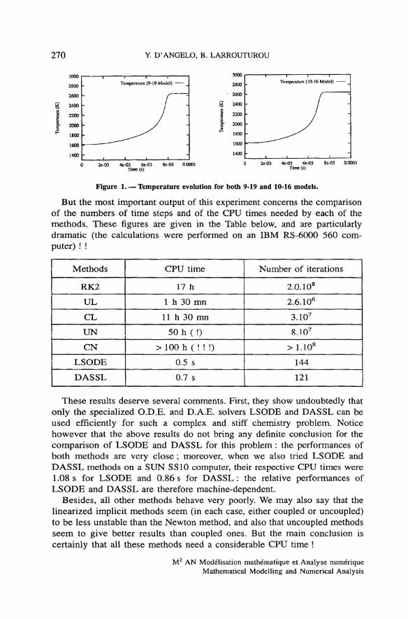
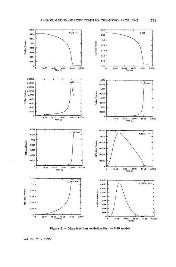
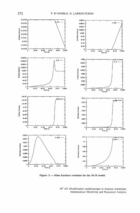
The numerical results obtained in this way are very similar for all methods(the plotted profiles are undistinguishable) and accurate. The time évolution ofthe température for both 9-19 and 10-16 chemistry models, presented onfigure 1, shows that the equilibrium température is reached slightly earlier withthe 10-16 mechanism than with the 9-19 model. The mass fractions profiles areshown on figure 2 for the 9-19 model, and on figure 3 for the 10-16 mecha-nism (for the latter, we have omitted the H2 and O2 profiles, which look verymuch like those on figure 2, but for the shorter equilibrium time). Notice that,for the 10-16 model, the species N2 and NO have not reached equilibrium atthe final time 10" 4 s.

vol 29, n° 3, 1995


4c-05 6c-05Time (s)

Be-05 0.0001 4C-G5 6c-05TimcCs)

8e-O5 0.0001

Figure 1. — Température évolution for both 9-19 and 10-16 models.

But the most important output of this experiment concerns the comparisonof the numbers of time steps and of the CPU times needed by each of themethods. These figures are given in the Table below, and are particularlydramatic (the calculations were performed on an IBM RS-6000 560 com-puter) ! !

Methods

RK2

UL

CL

UN

CN

LSODE

DASSL

CPU time

17 h

1 h 30 mn

11 h 30 mn

50 h (!)

> 100 h ( ! ! !)

0.5 s

0.7 s

Number of itérations

2,0.108

2.6.106

3.107

8J07

> L108

144

121

These results deserve several comments. First» they show undoubtedly thatonly the specialized O.D.E. and D.A.E. solvers LSODE and DASSL can beused efficiently for such a complex and stiff chemistry problem. Noticehowever that the above results do not bring any defmite conclusion for thecomparison of LSODE and DASSL for this problem : the performances ofboth methods are very close ; moreover, when we also tried LSODE andDASSL methods on a SUN SS10 computer, their respective CPU times were1.08s for LSODE and 0.86s for DASSL: the relative performances ofLSODE and DASSL are therefore machine-dependent.

Bes ides, ail other methods behave very poorly. We may also say that thelinearized implicit methods seem (in each case, either coupled or uncoupled)to be less unstable than the Newton method, and also that uncoupled methodsseem to give better results than coupled ones. But the main conclusion iscertainly that all these methods need a considérable CPU time !



4«-O5 6e-05Time (s)

ge-05 0.0001 4c-05 6e-05Time (s)

8e-05 0.0001

4c-05 6e-O5Time (s)

8e-O5 0.00014e-05 6e-05

Time (s)8e-05 0.0001

4e-0S 6e-0STime (s)

8e-O5 0.00010 2c-05 4e-05 6e-05 8e-05 0.0001

Time (s)

4e-05 6C-O5Time (s)

8e-O5 0.00014«-O5 6e-05

Tmre(s)8c-O5 0.0001

Figure 2. — Mass fractions évolution for the 9-19 model.

vol. 29, n° 3» 1995


2e-05 4e-O5 6e-O5 8e-O5 O.00O1Time (s)

2c-05 4e-05 6c-O5 8e-05 0.0001Time (s)

2e-05 4e-O5 6c-05 8c-05 0.0001Time (s) 2c-05 4«-05 6e-05

Time<s)8e-05 0,0001

2c-05 4«-05 ôe-05 8e-05 0.0001Time (s) 2e-05 4«-O5 6e-05 8e-05 0.0001

Time (s)

Figure 3. — Mass fractions évolution for the 10-16 model.

M2 AN Modélisation mathématique et Analyse numériqueMathematical Modeiling and Numerical Analysis


Before turning to our second numerical experiment, we should emphasizeagain two facts. On one hand, the above results are very far from beingoptimal, because we used a very poor strategy for adjusting the local timestep ; much better results will indeed be obtained in our third experimentbelow. On the other hand, it is worth to keep in mind that our sole criterionfor diminishing the time step in this experiment was the crash of the code. Wecould have decided to decrease Af whenever one of the mass fraction(s) wasbecoming négative (this actually happened during the calculation, but veryslightly ( ~ 1CT 7 in absolute value for the greater ones) ; the code crashedwhen more négative values were appearing). We will see in the next experi-ments that forcing the mass fractions to remain non négative would have ledto quite different results.

3.4. Second numerical experiment

We now investigate more closely the size of the time step with which eachof the methods can adequately operate. In our second experiment, we aregoing to détermine, for each method except LSODE and DASSL (but addingthe forward Euler explicit method), and for both 9-19 and 10-16 kineticmodels, the maximal time step required so as to ensure that all mass fractionsstay in the interval [0, 1]. This will be done for an initial pressure equal to theatmospheric pressure, and for an initial température increasing from 1 300 Kto 2 300 K with a step of 20 K.

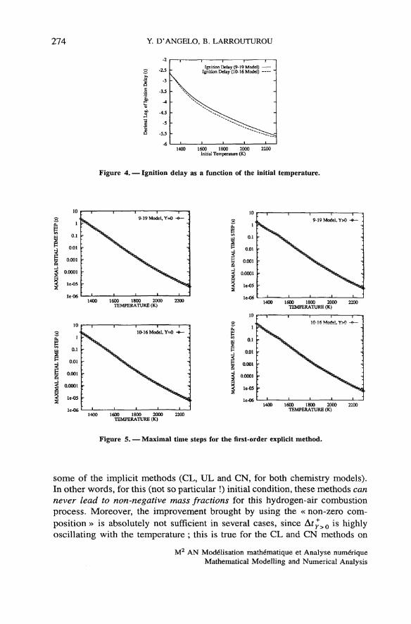
We will consider two different initial compositions. First, we take the sameinitial composition as in the above section, i.e. with zero mass fractions forspecies other than Hv O2 and N2. We wiil call this initial condition « zerocomposition» and the maximal allowed time step will be denoted Aty=0.Secondly, we leaded the same calculation by initiating the mass fractions withthe values calculated by LSODE at the time t = 10" 6 T, where T is the ignitiondelay at the considered température ; this initial condition will be called« non-zero composition », and the corresponding maximal time step is denotedAty>0. Let us make précise that we call hère « ignition delay » the time wherethe température profile changes its curvature (i.e. the inflection point), startingfrom the zéro-composition mixture ; this is a characteristic time for thecombustion of this mixture at a given température (see fig. 4).

The results are presented on figures 5 to 10.These results show for instance that using the « non-zero » initial mass

fractions does not necessarily increase the maximal usable time step, as wecould expect : we sometimes have Aty=ö> Aty>0 (and evenAty=Q> Aty>0 for the UN method).

But the most interesting resuit is that the initial time step Ar*=0 actuallyvanishes to zero (with machine accuracy) at some initial températures for

vol. 29, n° 3, 1995


Ignition Delay (9-19 Model) •Ignition Delay (10-16 Modcl) •

1400 1600 1800 2000Initial Température (K)

Figure 4. — Ignition delay as a function of the initial température.

1U

0.1

0.01

0.001

0.0001

le-05

-

-

-

1400

10

0.1

0.01

0.001

0.O001

le-O5

le-06

-

-

1400

9-19 Model, Y=© -«— ',

v •

^v -

1600 1800 2000 2200TEMPERATURE (K)

10-16 Model, Y=O -O— '.

1600 1800 2000 2200TEMPERATURE (K)

1600 1800 2000TEMPERATURE (K)

Figure 5. — Maximal time steps for the first-order explicit method.

some of the implicit methods (CL, UL and CN, for both chemistry models).In other words, for this (not so particular !) initial condition, these methods cannever lead to non-negative mass fractions for this hydrogen-air combustionprocess. Moreover, the improvement brought by using the « non-zero com-position » is absolutely not sufficient in several cases, since Af^>0 is highlyoscillating with the température ; this is true for the CL and CN methods on


APPROXIMATION OF STIFF COMPLEX CHEMISTRY PROBLEMS 2 7 5

1400 1600 1800 2000 2200TEMPERATURE (K) 1400 1600 1800 2000 2200

TEMPERATURE (K)

1400 1600 1800 2000 2200TEMPERATURE (K) 1400 1600 1800 2000 2200

TEMPERATURE (K)

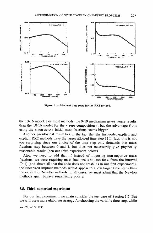
Figure 6. — Maximal time steps for the RK2 method.

the 10-16 model. For most methods, the 9-19 mechanism gives worse resultsthan the 10-16 model for the « zero composition », but the advantage fromusing the « non-zero » initial mass fractions seems bigger.

Another paradoxical resuit lies in the fact that the first-order explicit andexplicit RK2 methods have the larger allowed time step ! ! In fact, this is nottoo surprising since our choice of the time step only demands that massfractions stay between 0 and 1, but does not necessarily give physicallyreasonable results (see our third experiment below).

Also, we need to add that, if instead of imposing non-negative massfractions, we were requiring mass fractions « not too far » from the interval[0, 1] (and above all that the code does not crash, as in our flrst experiment),the linearized implicit methods would appear to allow larger time steps thanthe explicit or Newton methods. In ail cases, we must admit that the Newtonmethods again behave surprisingly poorly.

3.5, Third numerical experiment

For our last experiment, we again consider the test-case of Section 3.2. Butwe will use a more elaborate strategy for choosing the variable time step, while

vol. 29, n° 3, 1995


1400 1600 1800 2000 2200TEMPERATURE (K) 1400 1600 1800 2000 2200

TEMPERATURE (K)

1400 1600 1800 2000 2200TEMPERATURE (K) 1400 1600 1800 2000 2200

TEMPERATURE (K)

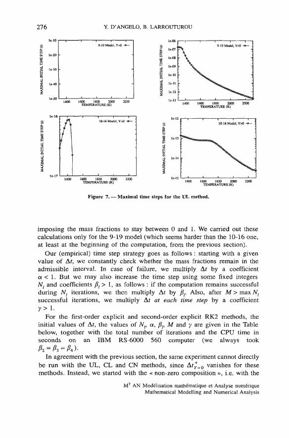
Figure 7. — Maximal time steps for the UL method.

imposing the mass fractions to stay between 0 and 1. We carried out thesecalculations only for the 9-19 model (which seems harder than the 10-16 one,at least at the beginning of the computation, from the previous section).

Our (empirical) time step strategy goes as follows : starting with a givenvalue of At, we constantly check whether the mass fractions remain in theadmissible interval. In case of failure, we multiply Af by a coefficienta < 1. But we may also increase the time step using some fixed integersNt and coefficients /?, > 1, as follows : if the computation remains successfulduring Nl itérations, we then multiply At by fir Also, after M > max Nl

successful itérations, we multiply At at each time step by a coefficienty>\.

For the first-order explicit and second-order explicit RK2 method s, theinitial values of At, the values of Nt, a, /?,, M and y are given in the Tablebelow, together with the total number of itérations and the CPU time inseconds on an IBM RS-6000 560 computer (we always took/?2 = /?3 = / ? 4 ) .

In agreement with the previous section, the same experiment cannot directlybe run with the UL, CL and CN methods, since Aty_0 vanishes for thesemethods. Instead, we started with the « non-zero composition », i.e. with the



§pi9 Naadel, f=<!

1400 1600 1800 2000 2200TEMPERATURE (K) 1600 1800 2000

TEMPERATURE (K)

Tl?

1600 1800 2000 2200TEMPERATURE (K) 1600 1800 2000 2200

TEMPERATURE (K)

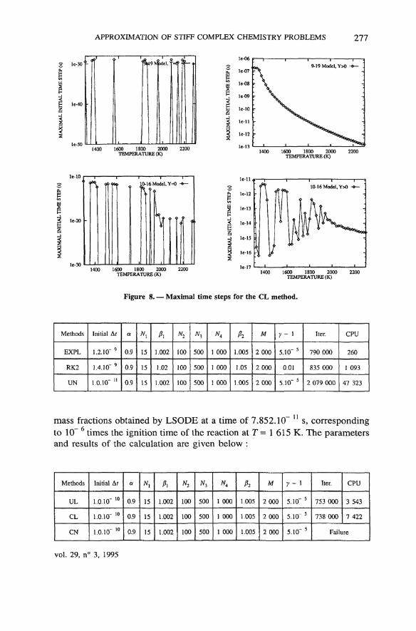
Figure 8. — Maximal time steps for the CL method.

Methods

EXPL

RK2

UN

Initial àt

1,2.10" 9

L4.10"9

L0.10- M

a

0.9

0.9

0.9

* i

15

15

15

A

1.002

1.02

1.002

100

100

100

N3

500

500

500

^ 4

1 000

î 000

1 000

h

1.005

1.05

1.005

M

2 000

2000

2000

y- i

5,10" 5

0.01

5.10" 5

ïter.

790 000

835 000

2 079 000

CPU

260

1 093

47 323

mass fractions obtained by LSODE at a time of 7.852.1Ö n s, correspondingto 10" 6 times the ignition time of the reaction at T= 1 615 K. The parametersand results of the calculation are given below :

Methods

UL

CL

CN

Initial àt

1.0.10" 10

1.0.10" 10

1.0.10" 10

a

0.9

0,9

0.9

15

15

15

A

1.002

1.002

1.002

N2

100

100

100

500

500

500

1 000

1 000

1 000

h

1.005

1.005

1.005

M

2000

2000

2000

y - 1

5.10" 5

5.10" 5

5.10" 5

ïter.

753 000

738 000

CPU

3 543

7 422

Failure

vol 29, n° 3, 1995




1400 1600 1800 2000 2200TEMPERATURE (K)

1400 1600 1800 2000 2200TEMPERATURE (K)

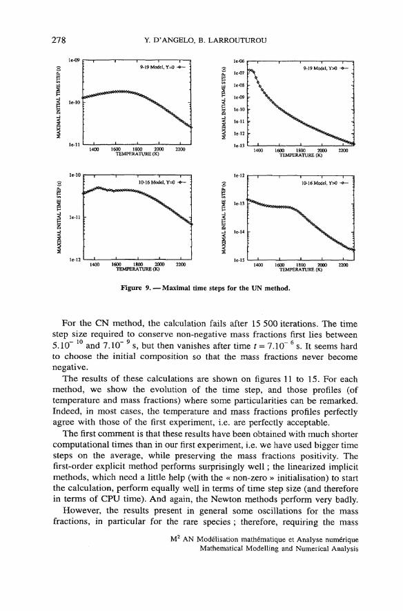
Figure 9. — Maximal time steps for the UN method.

For the CN method, the calculation fails after 15 500 itérations. The timestep size required to conserve non-negative mass fractions first lies between

r,- 10 Y- 95.10 and 7.10 s, but then vanishes after time t = 7.10 s. It seems hardto choose the initial composition so that the mass fractions never becomenégative.

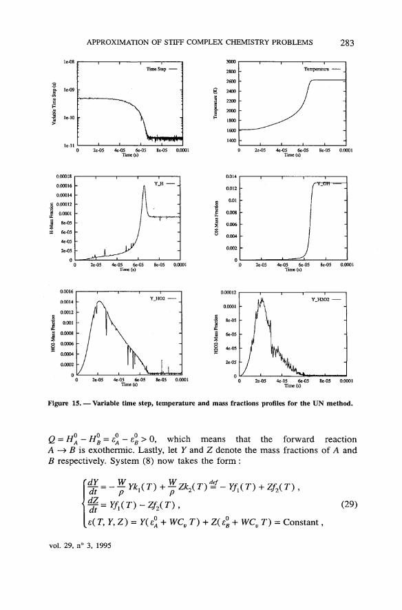
The results of these calculations are shown on figures 11 to 15. For eachmethod, we show the évolution of the time step, and those profiles (oftempérature and mass fractions) where some particularities can be remarked.Indeed, in most cases, the température and mass fractions profiles perfectlyagrée with those of the first experiment, i.e. are perfectly acceptable.

The first comment is that these results have been obtained with much shortercomputational times than in our first experiment, i.e. we have used bigger timesteps on the average, while preserving the mass fractions positivity. Thefirst-order explicit method performs surprisingly well ; the linearized implicitmethods, which need a little help (with the « non-zero » initialisation) to startthe calculation, perform equally well in terms of time step size (and thereforein terms of CPU time). And again, the Newton methods perform very badly.

However, the results present in gênerai some oscillations for the massfractions, in particular for the rare species ; therefore, requiring the mass

M2 AN Modélisation mathématique et Analyse numériqueMathematica! Modelling and Numerical Analysis


-S- le-30 9-19 Model, Y=0 -

1400 1600 1800 2000 2200TEMPERATURE (K)

1400 1600 1800 2000 2200TEMPERATURE (K)

V f > A

1400 1600 1800 2000 2200TEMPERATURE (K)

1400 1600 1800 2000 2200TEMPERATURE (K)

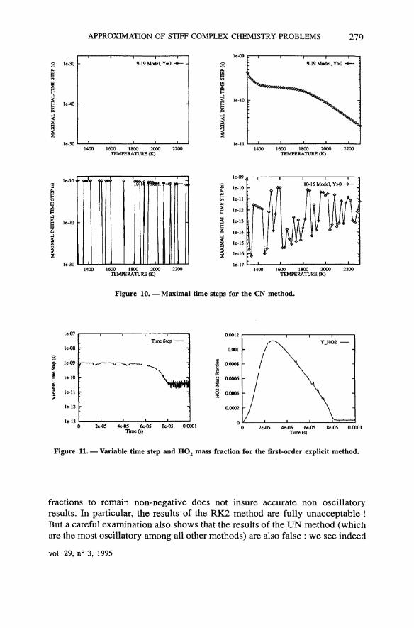
Figure 10. — Maximal time steps for the CN method.

le-07

lc-08

I Jc-09

^ le-10

le-12

le-13

Time Step -

0 2c-05 4e-05 6e-O5 8e-05 0.0001Time (s)

2e-05 4«-05 6c-05 8c-05 0.0001Time (s)

Figure 11. — Variable time step and HO2 mass fraction for the first-order explicit method.

fractions to remain non-negative does not insure accurate non oscillatoryresults. In particular, the results of the RK2 method are fully unacceptable !But a careful examination also shows that the results of the UN method (whichare the most oscillatory among ail other methods) are also false : we see indeed

vol. 29, n° 3, 1995


le-10

le-li

le-12

lc-13

lc-14

TîmeSiep -

0 2c-05 4e-05 6e-05 8e-05 0.0001Time (s)

4e-05 ôc-05Time (s)

8e-05 0.0001

4c-05 6c-05Time (s)

8e-05 0,0001 4e-05 6c-05Time (s)

8e-05 0.0001

0.005

0.0045

0.004

0.0035

0.003

0.0025

0.002

0.0015

0.001

0.0005

04c-05 6c-05

Time (s)8c-05 0.0001 4e-05 6e-05

Time (s)8c-05 0.0001

0 2e-05 4e-05 6e=05 8c-0S 0.0001Time (s)

2e-05 4e-05 6e-05 8e-O5 0.0001Time (s)

Figure 12. — Variable time step» température and mass fractions profiles for the RK2 method.

M2 AN Modélisation mathématique et Analyse numériqueMathematical Modellîng and Numerical Analysis


0 2e-05 4*-05 6c-05 8c-O5 0.0001Time (s)

4e-05 6e-05Time (s)

8e-05 0.0001

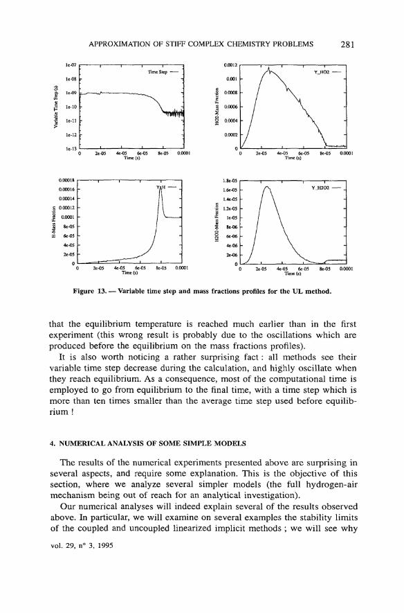
Figure 13. — Variable time step and mass fractions profiles for the UL method.

that the equilibrium température is reached much earlier than in the firstexperiment (this wrong resuit is probably due to the oscillations which areproduced before the equilibrium on the mass fractions profiles).

It is also worth noticing a rather surprising f act : all methods see theirvariable time step decrease during the calculation, and highly oscillate whenthey reach equilibrium. As a conséquence, most of the computational time isemployed to go from equilibrium to the final time, with a time step which ismore than ten times smaller than the average time step used before equilib-rium !

4. NUMERICAL ANALYSIS OF SOME SIMPLE MODELS

The results of the numerical experiments presented above are surprising inseveral aspects, and require some explanation. This is the objective of thissection, where we analyze several simpler models (the full hydrogen-airmechanism being out of reach for an analytical investigation).

Our numerical analyses will indeed explain several of the results observedabove. In particular, we will examine on several examples the stability limitsof the coupled and uncoupled linearized implicit methods ; we will see why

vol. 29, n° 3, 1995


0 2e-05 4e-05 6c-05 8e-05 0.0001Time (s)

2e-05 4e-05 6c-05 8e-O5 0.0001Time (s}

4e-05 6e-05Time (s)

8e-05 0.00014e-05 6e-05

Time (s)8e-O5 0.0001

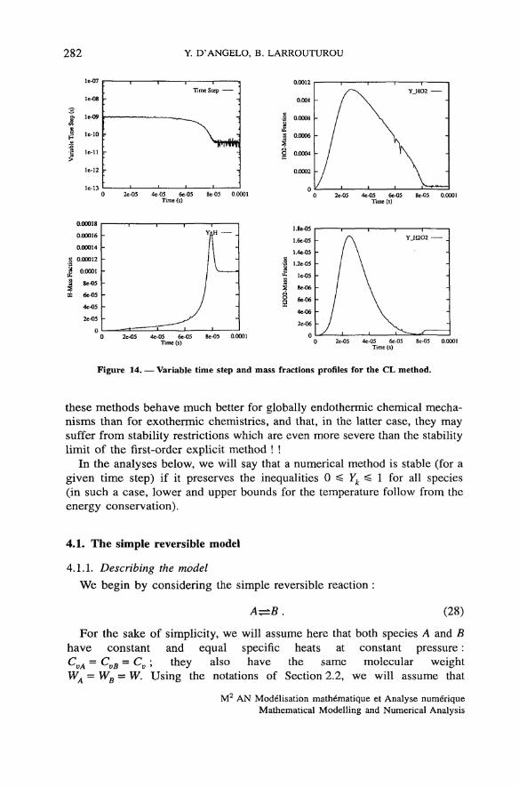
Figure 14. — Variable time step and mass fractions profiles for the CL method.

these methods behave much better for globally endothermic chenücal mecha-nisms than for exothermic chemistries, and that, in the latter case, they maysuffer from stability restrictions which are even more severe than the stabilitylimit of the first-order explicit rnethod ! !

In the analyses below, we will say that a numerical method is stable (for agiven time step) if it preserves the inequalities 0 ^ Yk ^ 1 for all species(in such a case, lower and upper bounds for the température follow from theenergy conservation).

4.1. The simple réversible model

4.1.1. Describing the modelWe begin by considering the simple réversible reaction :

A-B. (28)

For the sake of simplicity, we will assume here that both species A and Bhave constant and equal spécifie heats at constant pressure :CvA = CvB = Cv ; they also have the same molecular weightWA = WB - W. Using the notations of Section 2.2, we will assume that



0 2c-05 4c-05 6e-05 8e-05 0.0001Time (s)

4e-05 6e-05Time (s)

4e-05 6c-05Time (s)

8c-05 0.0001

0.014

0.012

0.01

0.008

0.006

0.004

0.002

04c-05 6e-05

Time (s)8e-O5 0.0001

4c-05 6c-05Tune (s)

8c-05 0.0001 0 2c-05 4e-05 6e-05 8c-05 0.0001Time (s)

Figure 15. — Variable time step, température and mass fractions profiles for the UN method.

Q = H0A - H°B = £° - e°B > 0, which means that the forward reaction

A —> B is exothermic. Lastly, let Y and Z dénote the mass fractions of A andB respectively. System (8) now takes the form :

{§=Yfl(T)-Zf2(T), (29)

e( T, Y, Z) = y( e° + WCV T) + Z( e°B+WCvT) = Constant,

vol. 29, n° 3, 1995


with

-^y, (30)

the fact that the two reaction rates f{ and f2 involve the same exponent ƒ?, aswell as the relation :

E2 = EX + Q, (31)

follow from the relations (13), (14) and (15).We recall that Cv and p are constant in System (29), and we set

QU = w r , . Obviously, any solution of this System satisfies the identifies :

y + Z = l , T + UY = Constant =f H° . (32)

Since ail numerical methods considered below also preserve these relations,we may simply rewrite the System (29) as :

UY = H° .

This System is completed with initial conditions: Y=Y°y T=T°.

Remark 4.1 : Below, we will sometimes need to consider realistic valuesfor the constants and variables of the problem. These values are obtained formthe following estimâtes and relations: we have Ke [0,1] ,T* [ 7 ^ . 7 ^ ] , with rmax = W°, ( r m a x - r m i n ) = t / ; typically, we haveT E7j^~5 to 8 and * ~4 to 10. Also, from Mayer's relation,-* min max _

( y — 1 ) WC = R, where y is the spécifie heat ratio yr-, *

Now, the differential form of the température équation, consistent with (33),writes :

g = UYf^T) -U(l- Y)f2(T) . (34)

In view of these relations, the région :

m, -{(y,ny/1(D-(i-F)/2(r)<o| (35)



of the ( Y, T) plane will be called the endothermic domain, whereas therégion :

> + = {( F, D , Yf{(T) - ( 1 - Y) f2( T) > 0} (36)

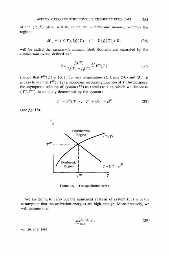
will be called the exothermic domain. Both domains are separated by theequilibrium curve, defined as :

y = def

MT)+f2(T)(37)

(notice that Y^(T) e [0, 1] for any température T). Using (30) and (31), itis easy to see that Ycq( T) is a monotone increasing function of T ; furthermore,the asymptotic solution of system (33) as t tends to + °°, which we dénote as( 7°°, r°°), is uniquely determined by the System :

(see fig. 16).

(38)

y - Y

Figure 16. — The equilibrium curve.

We are going to carry out the numerical analysis of System (33) with theassumption that the activation énergies are high enough. More precisely, wewill assume that :

(39)

vol. 29, n° 3, 1995


and also that :

P ^ 0 . (40)

4.1.2. Numerical analysisWe can now analyse how several of the numerical methods considered in

Section 3 behave when applied to the simple réversible model (28).We begin with the following simple resuit for the UN and UL methods.

PROPOSITION 4.2 : For the simple réversible reaction (28), the uncoupledNewton and uncoupled linearized methods are unconditionnally stable. •

Proof: Since System (33) is linear with respect to the mass fraction F, theUN and UL methods coincide in the present case. They take the form :

yn + 1 vnL / V^ ~^~

r + 1 , J J\7n "** 1 U^i KJ L — .fï

Then, we get :

and we easily see that Yn+X lies between 0 and 1 as soon as Yn does. •The situation is more complex for the CL method. We wilî prove the

following.

PROPOSITION 4.3 : For the simple réversible reaction (28), the coupledlinearized method is not unconditionnally stable.

However, if the assumptions (39) and (40) hold, then the coupled linearizedmethod is unconditionnally stable in the endothermic domain M_ . •

More précise statements will be made below about the actual stabilityrestrictions in the cases where unconditional stability does not hold, i.e. insome parts of the exothermic domain.

The proof of Proposition 4.3 consists of three Lemmas.

LEMMA 4.4 : Let ( 7n, Tn ) be the discrete température and mass fractioncomputed with the coupled linearized method.

There exists a <^?1 monotone increasing curve Y=Y*(T), with :

Y^iT) < y*(T)< 1 , (43)

such that 0 ^ Yn +1 ^ 1 for any At > 0 as soon aso ^ Yn < y*(r i). •



Proof : The CL scheme takes the form :

+ x - T") + ( 1 - y")f'1{Tn){Tn + l - Tn) ,

from which we get :

i U(- Ynf\{Tn) + (1 - 2

(45)

Assume now that Y" s [ 0 , 1 ] . If the term- Ynfl(T

n) + (1 - y " ) / 2 ( T " ) is non-negative, it is then clear that0 «Ï Y"+1 « 1 for any At > 0. This condition writes :

Y" ^ ^ L > «gY*{T"). (46)/î(r)+/2(r)

From the form (30) of fx and/2 , we get :

Y^p-, (47)for i = 1, 2. From (31), this shows that, for any T:

f\(T) M( 4 8 )

whence Y*(T) > 1^ (7 ) from (37) and (46). •Now, the endothermic domain ffl_ is a subset of the région {(Y,T),

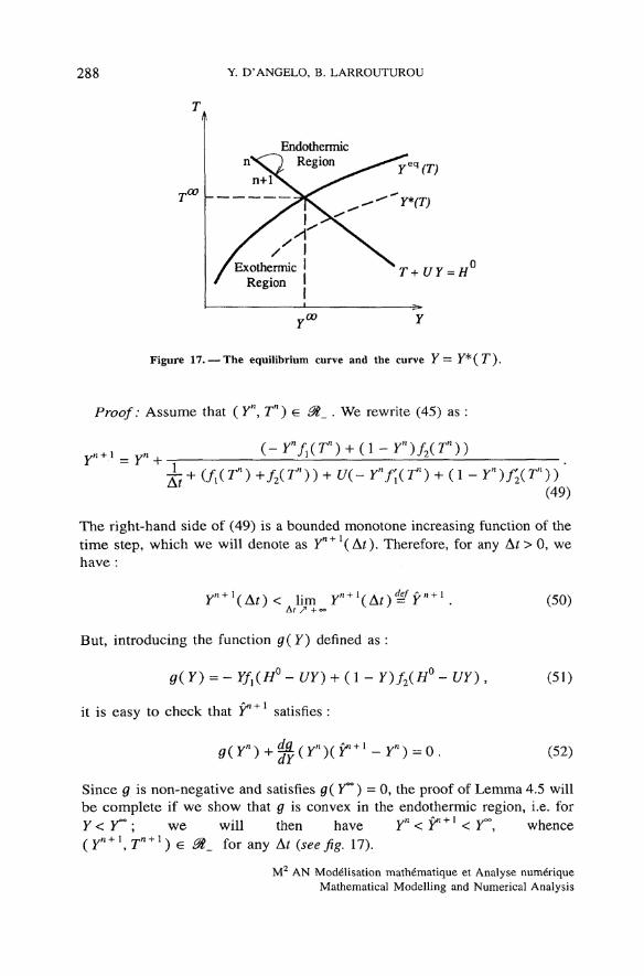
0 ^ y <: y*(7)} from (43), as shown on figure 17.Therefore, in order to show that the CL method is unconditionally stable in

the endothermic région, it remains to prove the following.

LEMMA 4.5 : Let (Yf\ Tn) be the discrete température and mass fractioncomputed with the coupled linearized method.

Assume that the technical assumptions (39) and (40) hold, and that0l_. Then, ( r + 1 , r + 1 ) e <%_. •

vol. 29, n° 3, 1995


EndothermicRégion

T+UY=H

rœ

Figure 17. — The equilibrium curve and the curve Y~ Y*(T).

Proof: Assume that ( Yn, Tn) e ^_ . We rewrite (45) as :

= Y" + •

a - r"(49)

The right-hand side of (49) is a bounded monotone increasing function of thetime step, which we will dénote as Yn* '(Aï). Therefore, for any Àt > 0, wehave :

y"+ 1(AO< lim Y"+[(At)=fY" + 1 .Ar /• + «s

But, introducing the function g(Y) defined as :

9( Y) = - Yf^H0 - UY) + ( 1 - Y)f2(H° - UY) ,

it is easy to check that Y"+ satisfies :

(50)

(51)

(52)

Since g is non-negative and satisfies g{ Y°° ) = 0, the proof of Lemma 4.5 willbe complete if we show that g is convex in the endothermic région, i.e. forY< Y~ ; we will then have Yn < Y" + 1 < F°°, whence(Yn+\ Tn+l) e m_ for any At (seefig. 17).



Let us therefore prove that g is convex in the endothermic région. For thesake of simplicity, we dénote TH( Y) - H° - UY, The first derivative ofg is given by :

ff'( Y) - - fx{ TH( Y) ) - / 2 ( TH( Y) ) - U[- Yf\{ TH( Y) ) +

H (53)

In the endothermic région, we have y < y * ( 7 H ( y ) ) from (43) and themonotonicity of y* (seefig. 17), which shows that the term between bracketsin (53) is positive. Therefore, g'(Y)<Q for Y< Y°°.

A second differentiation yields, after some algebra :

g'X Y ) = 2 u(f,(T"( y>) +f,(f{ rm

* ) <54>

Eiwith X: = B-\ s for i = 1,2. Usine (31), we can rewrite this as

1 /?rH(y)

Y) = 2 U(f\{TH( Y) ) + /2(TH( F) ) )

RTH( Y)

(55)

with

RTH(Y)J '

vol. 29, n° 3, 1995

290 Y. D'ANGELO, B. LARROUTUROÜ

In the endothermic domain, we know that - Yf^TH (Y)) +( 1 - Y)f2(T

H(Y)) > 0. Therefore, g\Y) will be proved to be positive ifwe show that :

and il - XÏ TT— ̂ O . (56)

Regarding the second expression in (56) as a second-order polynomial in thevariable Xz> w e c a n rewrite these two conditions as :

and M2RTH(Y) A2 RTH(Y)"2 "V RTH(H) 4"(57)

After some simple algebra, using the assumption (40) on 0, one easily checksthat the last condition in (57) is equivallent to : 2RTH(Y) ^ Ev Bothconditions (57) are then fulfilled from (39), which ends the proof. •

Remark 4.6 : It is easy to see from the above proof that the same conclu-sions can be reached even if 0 < 0s but with a stronger hypothesis than (39)on the activation énergies. For instance» the above results remain true if theconditions (39)-(4Ö) are replaced by :

and 2 RT ^ min I * A z , — I . • (58)

Max i A * -c / \ /

Remark 4,7: In fact, the preceding proofs show that the CL method isunconditionally stable as soon as the initial condition satisfiesY0 ̂ F*(T°). Indeed, if the initial data lie above the curve F= Y*(T) butin the exothermic domain, we know that Ö ̂ Fn + Î *S 1 for anyAt>0, and (49) shows that Fr t+1<FM. This means that the séquence( F" ) is decreasing for n small enough, Then» either this séquence alwaysdecreases» which means that ( Y'\ Tn) e M + and Yn < Y*(Tn) for ail «, andthe scheme is unconditionally stable from Lemma 4.4 ; or there exists n0 suchthat (Y#H>,7rfl0)G 0t_ and, for n > nö> the séquence (Fw) increases but( Yn

f Tn) remains in the endothermic domain from Lemma 4.5. In both cases,

we have :

Mm Y^^Y00, lim f = T . • (59)y*+oo B/+CO



To conclude our analysis, it remains to examine why the CL method is notunconditionally stable in the whole exothermic domain. This is the object ofthe next Lemma.

LEMMA 4.8 : The coupled linearized method is not always unconditionnallystable for the simple réversible reaction (28). •

Proof : In Lemma 4.4, we have written only a sufficient condition for thestability of the method. Now, returning to (45) and assuming that0 ^ Yn ^ 1, it is easy to see that the property :

0 ^ Yn+1 ^ 1 V A r > 0 (60)

is achieved if the following two necessary and sufficient conditions aresatisfied :

f f2(Tn) + UY\- Ynf[(Tn) + (1 - Yn)f2(T

n)) > 0 ,

1/(7*) + U( 1 - Y")(- Ynf[(Tn) + (1 - Yn)f2(Tn) ) ^ 0 .

Writing the first inequality as AX(Y) = (f[ + f2) Y1 - f'2Y - ^ ^ 0 , we

2 4flsee that the discriminant of Av A(Al)=f2 +-77-(ƒ!+/^), is alwayspositive, and that Ax has exactly one positive root. The first condition in (61)may therefore be written under the form :

Yn ^ <&}(Tn). (62)

With realistic values for Ev Q and T (see Remark 4.1), Ax( 1 ) is positive,which means that 0 < ^ 1 ( 7 ) < l and that (62) introduces an actualrestriction.

The second inequality in (61) leads to :

A2(Y) = (f\ +f2) Y2-(2f2+f\)Y +

fjj+f2 ̂ 0 . (63)

2 4AThe discriminant of A2 is A(A2) =f\ - -JJ- (f\ +f2). Again, withrealistic values for Ev Q and T, this expression is positive. Examining thevalues of A2( 0 ), A2{ 0 ), A2( 1 ), A2( 1 ), it is easy to see that A2 has two rootsinside the interval [0, 1], which means that the second condition in (61) isequivalent to a condition of the form :

y-« [ » 2 ( r ) , ^ 3 ( r ) ] , (64)

vol. 29, n° 3, 1995


with 0<<The two conditions (62)-(64) show that the CL scheme is not uncondition-

ally stable. •We will not try to exploit any further the conditions (62)-(64), which are

quite heavy to handle with. Instead, we will now examine the simpler case ofa non-réversible reaction.

4.2. The one-step reaction

For the sake of simplicity, let us now consider the simplest case of a singleone-step reaction A ~^> B. Keeping the same notations as above, we will simplyassume that A2 = 0 in (30). Our aim hère is to compare the stabilityrestrictions for the linearized implicit schemes and the flrst-order explicitscheme.

We easily have :

Yn + l = Yn(l~ àtfx{Tn)) (65)

for the explicit forward Euler scheme,

vn

r+1 = (66)

for the UL method, which is still unconditionally stable, and :

(67)

for the CL scheme. It is then easy to see that the explicit method (65) is stableunder the condition :

(68)

whereas the CL method is stable under the following condition (if

UYnfx(Tn)

(69)



Then, the ratio of these two limiting values of the time step is :

ArCL fATn) Tn x x: r ZTT— ~n — Î (70)

r RTn

we have used Remark 4.1 and (47). It is then clear that this ratio can besubstantially smaller than 1 : the stability restriction of the coupled linearizedimplicit method is then strictly more severe than the stability limit of theexplicit Euler forward scheme ! !

4.3. Global hydrogen-oxygen reactions

We will now analyse further the UL method, which we found to beunconditionnally stable for the simple réversible model (28), for two globalformulations of the hydrogen-oxygen combustion. In fact, we will consider thetwo following réversible models :

2 (71)

and

H2 + ±O 2 —H 2 O, (72)

and we will show that, surprisingly, the application of the uncoupled linearizedmethod to (71) and (72) leads to very different stability limits.

4.3.1. The model with integer stoechiometric coefficients

Let us begin with the first model (71).Calling X, Y and Z the mass fractions of H2, O2 and H2O respectively, and

fx(T) and f2(T) the forward and reverse reaction rates, we are led to thesystem :

X = -2WH2(X2Yfl-Z

2f2),

Y=-WO2(X2Yfx-Z

2f2), (73)

Z=-2WH2O(X2Yfx-Z2f2).

We then have the following result.

PROPOSITION 4.9 : For the global réversible reaction (71), the uncoupledlinearized method is unconditionnally stable : if Xn, Yn, Zn ^ 0and Xn + Yn + Zn = 1, then Xn+\ Yn+\ Zn+l ^ 0 andXn + 1 + rrt + 1 + Z " + 1 = l for any Af. •

vol. 29, n° 3, 1995


Proof: Writing ÔF = Fn+l ~Fn for F = X, Y or Z, we may write theUL method for the mas s fraction X as :

g = - 2 WH2[(X2 F/T - Z 2 / 2 ) + 2X7/! ̂ + X2 / ! < ^ - 2Z/2<5Z] . (74)

We have omitted the superscripts n for Xn, Yn and Zn in the right-hand side ofWo2 WU20

this relation. Moreover, we have öY^-^W—&% anc* ^~~~w—"X from(73). After a straightforward calculation, we obtain,

^ + (4 WH2XY+ WOiX2)Â + 4 ^H2O

^ + (4 WHiXY+ WO2X2)fl+4Wll2OZf2

WHiXYZ)fx + (2

(75)

Now, assume that X\ Yf\ Zn ^ 0 and that X" + Yn + Zrt = 1. It is thenobvious that Xn + \ Yn + \ Zn+l ^ 0 for any Ar > 0. Moreover, using therelation 2 WH2 + WOi = 2 WHn 0 , it is easy to check that

n +1 n +1 2n +1 : c o m p ie tes the proof. •

4.3.2. T/ie model with non-integer stoechiometric coefficients

Considering now the second model (72) and using the same notations, weobtain the system :

X=-WH2(xVYfx-Zf2),w^ ( V ? ) (76)

We then have the following resuit, which says that the UL method is notunconditionnally stable for this model.



PROPOSITION 4.10 : For the global réversible reaction (72), the uncoupledlinearized method is not unconditionally stable. The stability condition writes :

Wo X Wo Z

for Y > 0. •

Proof : After some algebra, we find that the application of the UL methodto (76) leads to :

r- WO*

ytl+l __

XVf zwo

7 / Wa XZAf \ H2 4 \^J

^H2o/2

(78)

The arguments are then the same as in the preceding proof : assuming thatX\ Y\ Zn^0 and that X B + y " + Z " = l , it is obvious that, for anyAt > 0, we have Xn + l & 0, Zfl + 1 ^ 0 and Xn + l + Fn + 1 + Z n + 1 = 1. Also,it is clear that Yn+l ^ 0 if and only if (77) holds, which complètes theproof, •

Remark 4.11 : Let us comment about the stability condition (77). It is clearthat» if X is small enough» i.e. for sufficiently lean mixtures, the UL schemeis unconditionnally stable (the right-hand side of (77) is then négative). On theother hand, for rich mixtures, i.e. for Y small enough, there is an actuallimitation on At, which takes the form (at the leading order) :

At4vf

'UL ' (79)

voL 29, n° 3, 1995


On the other hand, it is readily seen in this case that the stability limit of theexplicit forward Euler scheme reads :

(80)

Thus, for very rich mixtures» the uncoupled linearized method may operatewith time steps which are only twice greater than the time step allowed for theexplicit method. •

4.4. Â remark about the fractional-step approach

The previous sections show on the basis of the analysis of several tractablemodels that the linearized implicit methods suffer from very severe stabilityrestrictions for the intégration of the chemical model (8). One may thenwonder whether this result is not due, at least partly, to our fractional-stepapproach. In other words, may the linearized implicit schemes operate withlarger time steps if, instead of considering the sole chemical source terms, wesimultaneously integrate the convective (and possibly the diffusive) termstogether with the chemical terms ?

The answer to this question is négative : the stability limit of the linearizedimplicit methods for the coupled convective-reactive system is not any greaterthan the stability limit of these schemes for the purely chemical system (8).This fact is illustrated by the following example, where we consider the mostsimple convective-reactive system for a one-step reaction A —» B, with con-stant velocity and constant energy :

Assurrüng for the sake of clarity that uQ > 0 and setting againTH( Y) = H°- UY, we have (compare with (69)).

LEMMA 4.12: For the solution of (81), the upwind linearized implicitscheme :

At +U° Ax

1 fx(TH(Yn.)) + UY]fï(T

H(Yi))(Y]+i- Y]) (82)



is stable under the condition :

At ^ î— . • (83)t/^/Ï^Cyp)

Proof : The scheme (82) can be written in matrix form as+ 1 \ with:

(84)

ail other terms being zero. Clearly, if (83) holds, then & ^ 0, and se is anM-matrix (sfu > 0 for ail j , sfJtk^0 for j =* k and 2 ^ * > 0 for ail2j ; see [11]). As a conséquence, j / ~ l ^ 0, whence Fn + 1 ^ 0 as soon asYn 5* 0.

If (83) holds, we may also set V - $~ l se and write the scheme (82) as<gYn+l = Yn. Then, ^ is an M-matrix and, denoting 1 the vector whosecomponents are ail equal to unity, we easily see that # 1 ^ 1 . Thus,V l 5= 0 and we have #~ l 1 ^ 1. Assuming that Yn ^ 1, we see thatYn + X = <ë~l Yn ^ 1, which ends the proof: the inequalities0 ^ y j + 1 ^ 1 hold for ail j . •

5. CONCLUSIONS

We have investigated in this paper the use of the nonlinear implicit andlinearized implicit methods for the time intégration of exothermic complexchemistry models.

We have enlightened the inefficiency of these methods through threenumerical experiments, which showed (i) that a straightforward use of thesemethods leads to prohibitive computation times for the simulation of hydrogencombustion, (ii) that, for some initial conditions, several of these methods areunable to preserve the mas s fractions positivity, even with extremely smalltime steps, and, more importantly and more surprisingly, (iii) that monitoringthe time step for these calculations by only requiring the préservation of themass fractions positivity may lead to physically unacceptable results.

We explained these observations by analysing the behaviour of the linear-ized implicit methods for several (not too complex) tractable chemical mecha-nisms. These analyses show that the stability limit of the linearized implicitmethods strongly depend on the detailed form of the chemical model. Also,

vol. 29, n° 3, 1995

298 Y- D'ANGELO, B. LARROUTUROU

they explain in a convincing way that the linearized implicit methods are notsuitable for the time intégration of exothermic chemical mechanisms, whereasthey are known to be adequate for endothermic chemistries (see [2, 3, 8]).

Remark 5.1 : The nonlinear implicit methods deserve some further com-ments. Following the arguments used in [4], it can indeed be shown that, forany time step At9 as soon as the nonlinear discrete System to be solved in thesemethods has a solution (F j t)"+Î, Trt+1, then this solution satisfies the maxi-mum principle : 0 ^ Yn

k+l ^ 1 (and this remains true if convective and

diffusive terms are added ; see [4]). Therefore, the instabilities observed forthese methods in our experiments should be interpreted as the divergence ofthe Newton itérations for the solution of the nonlinear discrete problem, notas an intrinsic instability of the nonlinear formulation itself. It might in fact bethe case that this situation can be improved by using another itérativetechnique instead of Newton method (such as damped Newton, GMRES, ...)>or by coupling the convective or diffusive terms with the chemical sourceterms within the itérations (see e.g. [10]). •



APPENDIX

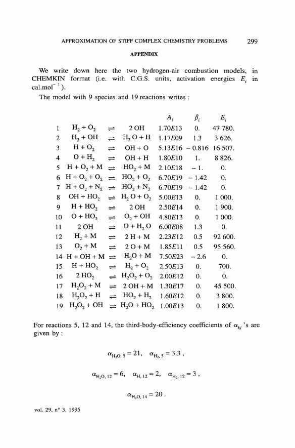
We write down here the two hydrogen-air combustion models, inCHEMKEN format (i.e. with C.G.S. units, activation énergies Ei incal.moF ! ).

The model with 9 species and 19 reactions writes :

1

2

3

4

5

6

7

8

9

10

11

12

13

14

15

16

17

18

19

H2 + O2 ^

H2 + OH —

H + O2 —

O + H2 —

H + O2 + M —

H + O 2 + O2 —

H + O2 + N2 —

OH + HO2 —

H + HO2 ^±

O + HO2 —

2 OH —H2 + M —

O2 + M ^

H + OH + M —H + HO2 —

2HO2 —

H2O2 + M —

H2O2 + H —

H2O2 + OH —

2 OHH2O + H

OH + O

OH + HHO2 + M

HO2 + O2

HO2 + N2

H2 O + O2

2 OHO2 + OH

O + H2O

2H + M

2O + MH2O + M

H2 + O2

H2°2 + °22OH + MHO2 + H2

H2O + HO2

A-1.70E13

1.17E09

5.13E16

1.80£10

2.10E18

6.70E19

6.70E19

5.00£13

2.50£14

4.80E13

6.00E08

2.23E12

1.85E11

7.50£23

2.50E13

2.00E12

1.30E17

1.60E12

1.00JS13

Pi0.

1.3

-0.816

1.

- 1.

- 1.42

- 1.42

0.

0.

0.

1.3

0.5

0.5

- 2 . 6

0.

0.

0.

0.

0.

Al 780.

3 626.

16 507.

8 826.

0.

0.

0.

1000.

1 900.

1 000.

0.

92 600.

95 560.

0.

700.

0.

45 500.

3 800.

1 800.

For reactions 5, 12 and 14, the third-body-efficiency coefficients of a.ki 's aregiven by :

H2O, 12 = "» aH, 12 = 2 ' a H 2 ( 12

«H2O, 14 = 2 0 *

vol. 29, n° 3, 1995


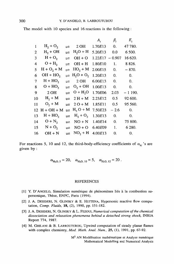
The model with 10 species and 16 reactions is the following :

1

2

3

4

5

6

7

8

9

10

11

12

13

14

15

16

H2-

H2-

H H

O H

+ O2 ^f OH ^±

hO2 -hH2 ^

H + O2 + M -OH-

H +O +

2H2

O2

hHO2 ^HO2 ^±HO2 ^±

OH —+ M ^±+ M ^

H + OH + M ^±H +O -

N -

OB

HO2 —f N2 —fO 2 ^

[ + N ^±

2 OHH2O + H

OH + OOH + H

HO2 + MH2O + O2

2 OHO2 + OHO + H2O

2 H + M2O + M

H 2 0 + MH2 + O2

NO + NNO + ONO2 + H

Ai

1.70M35.20E131.22E171.80£102.00E151.20E136.00£131.00^131.70^062.23E121.85E117.50E231.30^131.40E146.40^094.00£13

A0.

0.0

- 0.9071.

0.

0.

0.

0,

2.030.5

0.5

-2 .60.

0.

1.

0.

Ei

47 780.6 500.16 620.8 826.-870.

0.

0.

0.

- 1 19092 600.95 560.

0.

0.

75 800.6 280.

0.

For reactions 5, 10 and 12, the third-body-efficiency coefficients of a.ki 's aregiven by :

aH2O, 5 = 20» <*H2O, 10 ~ 5> «H2O, 12 = ™ •

REFERENCES

[1] Y. D'ANGELO, Simulation numérique de phénomènes liés à la combustion su-personique, Thèse, ENPC, Paris (1994).

[2] J. A. DESIDERI, N. GLINSKY & E. HETTENA, Hypersonic reactive flow compu-tation, Comp. Fluids, 18, (2), 1990, pp. 151-182.

[3] J. A. DESIDERI, N. GLINSKY & L. FEZOUI, Numerical computation ofthe chemicaldissociation and relaxation phenomena behind a detached strong shock, INRIAReport 774, 1987.

[4] M. GHILANI & B. LARROUTUROU, Upwind computation of steady planar flameswith complex chemistry, Mod. Math. Anal Num., 25, (1), 1991, pp. 67-92.



[5] A. C. HlNDMARSH, ODEPACK, a systematized collection of ODE solvers, IMACSTrans, on Se. Comp., Stepleman et al. eds., pp. 55-64, North-Holland, Amster-dam, 1983.

[6] R. J. KEE, J. A. MILLER & T. H. JEFFERSON, CHEMKIN ; a gênerai purpose,problem-independent, transportable, FORTRAN chemical kinetics code package,SANDIA Report SAND83-8209, 1983.

[7] B. LARROUTUROU, HOW to preserve mass fractions positivity when Computingcompressible multi-component flows, / . Comp. Phys., 95, (1), 1991, pp. 59-84.

[8] C. P. Ll, Implicit methods for Computing chemically reacting flows, NASA Techn.Mem. 58274, Houston, 1986.

[9] L. R. PETZOLD, A Description of DASSL : a differential/algebraic System solver,IMACS Trans, on Se. Comp., Stepleman et al. eds., North-Holland, Amsterdam,1983.

[10] M. D. SMOOKE, A. A. TURNBULL, R. E. MiTCHELL SL D. E. KEYES, Solution oftwo-dimensional axisymmetric laminar diffusion fiâmes by adaptive boundaryvalue methods, Mathematical modelling in combustion and related topics, Brau-ner & Schmidt-Lainé eds., pp. 261-300, NATO ASI Series E, Nijhoff, Doordrecht,1988.

[11] R. S. VARGA, Matrix itérative analysis, Prentice Hall, 1962.

[12] F. M. WHITE, Viscous fluid flow (second édition), McGraw-Hill, New-York, 1991.

vol. 29, n° 3, 1995

Comparison and analysis of some numerical schemes … · APPROXIMATION OF STIFF COMPLEX CHEMISTRY...

Documents

Transcript of Comparison and analysis of some numerical schemes … · APPROXIMATION OF STIFF COMPLEX CHEMISTRY...