Climate change effects on extreme precipitation in Morocco

Yves Tramblay, Luc Neppel, Eric ServatHydroSciences Montpellier, UMR 5569 (CNRS-IRD-UM1-UM2), France

Wafae Badi, Fatima DriouechDirection de la Météorologie Nationale, Centre National de Recherche Météorologique, Casablanca, Maroc

Salah El AdlouniInstitut National de Statistique Appliquée, Rabat, Maroc

Département de Mathématique et Statistique, Université de Moncton, Canada

Objectives

Morocco is often hot by intense rainfall events, causing human losses and economic damages (ex. Ourika, 1995, Rabat, Casablanca, Tanger, 2009)

Goals of the study:

1- Evaluate the past trends in the observed extreme precipitation records and the dependences with circulation indexes (NAO, MO)

2- Evaluate the possible future trends with outputs of different Regional Climate Models (RCM) from the ENSEMBLE project (www.ensembles-eu.org)

1- Datasets and methods

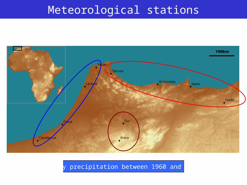
Meteorological stations

Daily precipitation between 1960 and 2007

Global and Regional Climate Models

• Higher spatial resolution = better description of orography• Responds in a physically consistent way to different forcings• Better reproduce extreme events than GCMs (Frei, 2006, Fowler, 2007)

• Dependent on the boundary conditions imposed by the parent GCM• Requires advanced computing resources

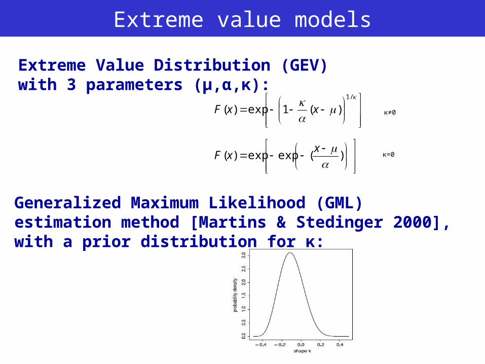
Extreme value models

/1

)(1exp)( xxF

)(expexp)(

x

xF κ=0

κ≠0

Extreme Value Distribution (GEV) with 3 parameters (µ,α,κ):

Generalized Maximum Likelihood (GML) estimation method [Martins & Stedinger 2000], with a prior distribution for κ:

2- Past trends

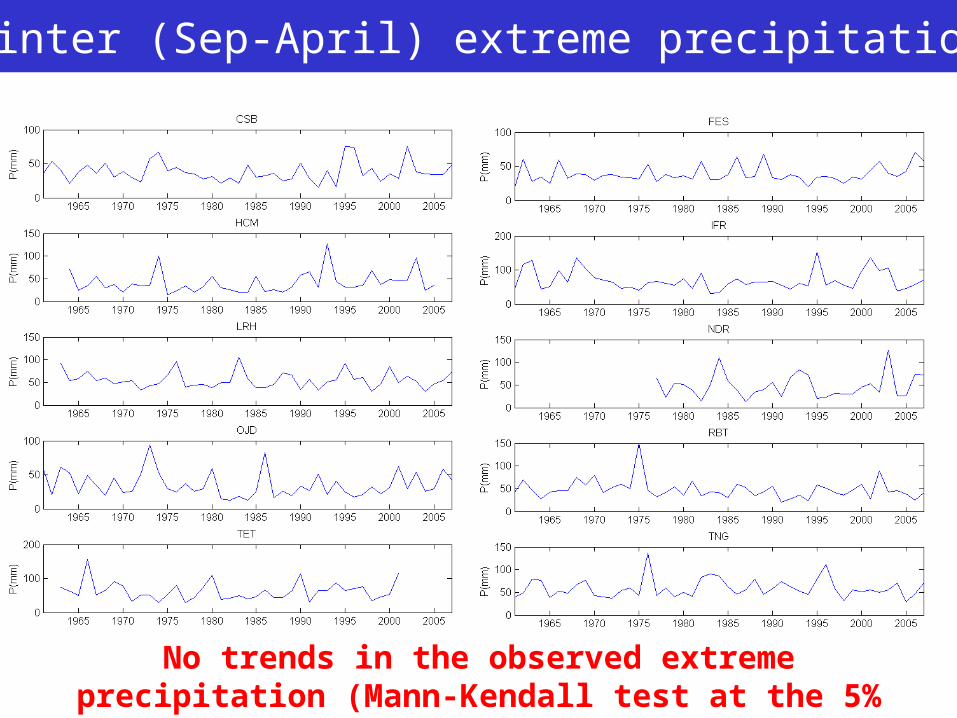
Winter (Sep-April) extreme precipitation

No trends in the observed extreme precipitation (Mann-Kendall test at the 5% level)

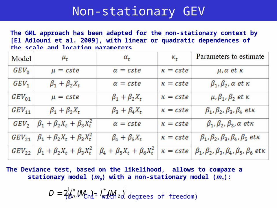
Non-stationary GEV

The GML approach has been adapted for the non-stationary context by [El Adlouni et al. 2009], with linear or quadratic dependences of the scale and location parameters

)()(2 0*

1* MlMlD nn

The Deviance test, based on the likelihood, allows to compare a stationary model (m0) with a non-stationary model (m1):

(D ~ Chi² with ʋ degrees of freedom)

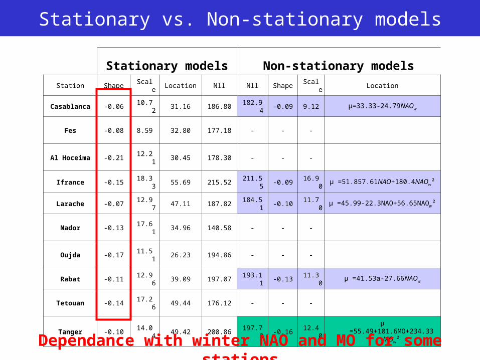
Stationary vs. Non-stationary models

Stationary models Non-stationary modelsStation Shape Scale Location Nll Nll Shape Scale Location

Casablanca -0.06 10.72 31.16 186.80 182.94 -0.09 9.12 μ=33.33-24.79NAOw

Fes -0.08 8.59 32.80 177.18 - - -

Al Hoceima -0.21 12.21 30.45 178.30 - - -

Ifrance -0.15 18.33 55.69 215.52 211.55 -0.09 16.90 μ =51.857.61NAO+180.4NAOw²

Larache -0.07 12.97 47.11 187.82 184.51 -0.10 11.70 μ =45.99-22.3NAO+56.65NAOw²

Nador -0.13 17.61 34.96 140.58 - - -

Oujda -0.17 11.51 26.23 194.86 - - -

Rabat -0.11 12.96 39.09 197.07 193.11 -0.13 11.30 μ =41.53a-27.66NAOw

Tetouan -0.14 17.26 49.44 176.12 - - -

Tanger -0.10 14.04 49.42 200.86 197.72 -0.16 12.40 μ =55.49+101.6MO+234.33MOw²

Dependance with winter NAO and MO for some stations

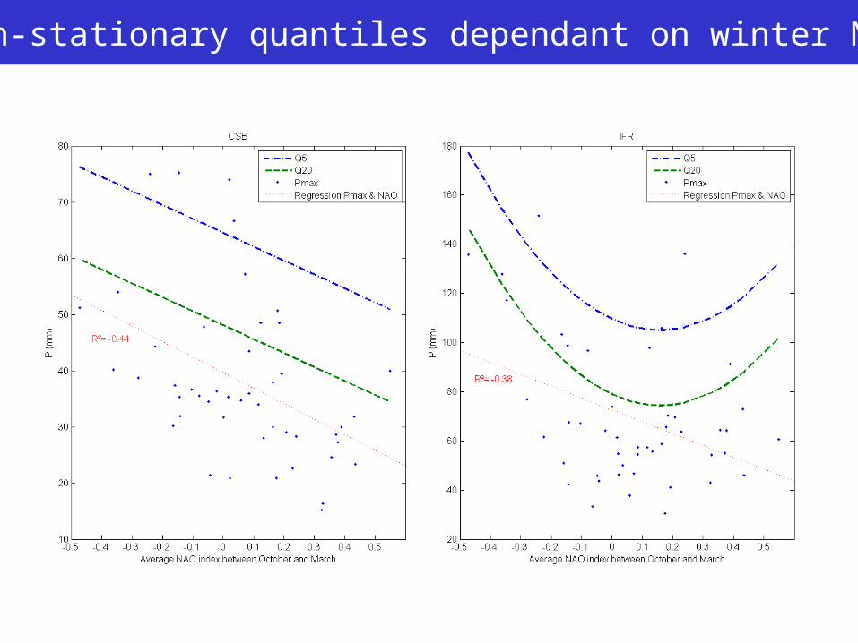
Non-stationary quantiles dependant on winter NAO

3- Evaluation of RCM outputs

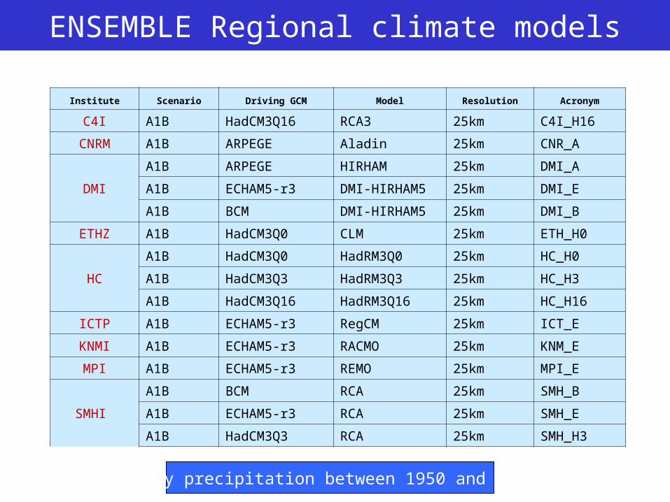
ENSEMBLE Regional climate models

Institute Scenario Driving GCM Model Resolution Acronym

C4I A1B HadCM3Q16 RCA3 25km C4I_H16

CNRM A1B ARPEGE Aladin 25km CNR_A

DMI

A1B ARPEGE HIRHAM 25km DMI_A

A1B ECHAM5-r3 DMI-HIRHAM5 25km DMI_E

A1B BCM DMI-HIRHAM5 25km DMI_B

ETHZ A1B HadCM3Q0 CLM 25km ETH_H0

HC

A1B HadCM3Q0 HadRM3Q0 25km HC_H0

A1B HadCM3Q3 HadRM3Q3 25km HC_H3

A1B HadCM3Q16 HadRM3Q16 25km HC_H16

ICTP A1B ECHAM5-r3 RegCM 25km ICT_E

KNMI A1B ECHAM5-r3 RACMO 25km KNM_E

MPI A1B ECHAM5-r3 REMO 25km MPI_E

SMHI

A1B BCM RCA 25km SMH_B

A1B ECHAM5-r3 RCA 25km SMH_E

A1B HadCM3Q3 RCA 25km SMH_H3

Daily precipitation between 1950 and 2100

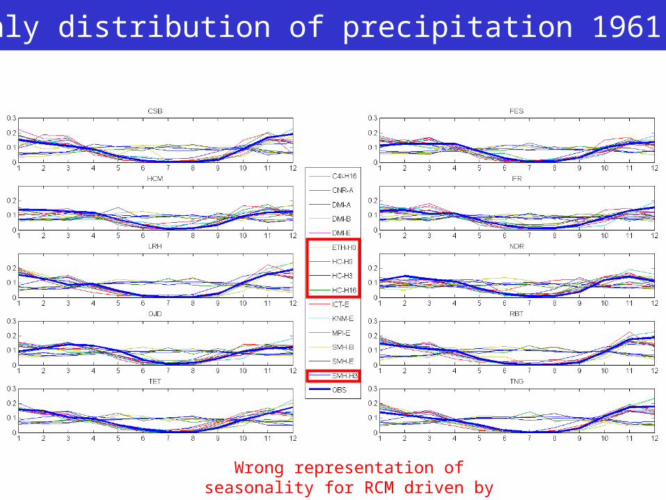
Monthly distribution of precipitation 1961-2007

Wrong representation of seasonality for RCM driven by HadCM

Extreme precipitation distributionThe distribution of observed extremes is compared with the distribution

simulated by the different RCMs

Similar distributions, but RCMs underestimate extreme precipitation

Cramér-von Mises test

)(²),()(² xdFxFxFn

)(²)()()/( xdHxGxFMNNMD mnmn

Goodness-of-fitF(x,θ) = fitted

Fn(x) = empirical

Distance between two empirical distributions

Fn(x) = empirical

Gm(x) = empirical

The statistical significance of the differences can be computed by bootstrap

= Quadratic distance between two distributions (specified or not)

Cramér-von Mises (CM) statistic

The CM statistic is computed between observed and RCM distributions

Can provide weights to combine the different model outputs

5- Future trends

Methodology

1961-2007 2020-2050 2070-2099

GEV fit GEV fit GEV fit

Scaling factor for 2020-2050 = Qp1 / Qo

Scaling factor for 2070-2099 = Qp2 / Qo

Quantile Qo Quantile Qp1 Quantile Qp2

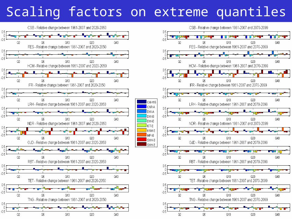
Scaling factors on extreme quantiles

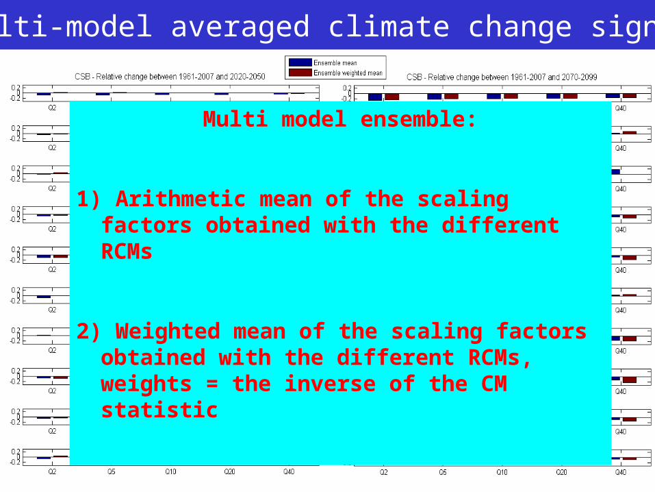
Multi-model averaged climate change signal

Multi model ensemble:

1) Arithmetic mean of the scaling factors obtained with the different RCMs

2) Weighted mean of the scaling factors obtained with the different RCMs, weights = the inverse of the CM statistic

Conclusions

1. No trend identified during the observation period. Dependences between precipitation extremes with NAO and MO indexes, in particular for the Atlantic stations

2. Great variability in the RCM performances to reproduce the annual cycles and the extreme precipitation distributions. Some models have good skills, with simulated and observed extreme distributions not statistically different

3. The climate change signal in the RCM simulations indicate a decrease in extreme precipitation in particular for the projection period 2070-2099, and a great variability and lower convergence between the models for the projection period 2020-2050

4. Good model convergence towards a decrease for the Atlantic stations. For the Mediterranean stations, the projected changes are difficult to assess due to the great variability.

5. The two weighting schemes tested for model outputs provide similar results

Thanks for your attention

Contact: ytramblay@gmail.com

Reference :

Tramblay, Y., Badi, W., Driouech, F., El Adlouni, S., Neppel, L., Servat, E., Global and Planetary Change, 2011, submitted