characterization of on-line sensors for water - Universit© Laval
151
Mathieu Beaupré CHARACTERIZATION OF ON-LINE SENSORS FOR WATER QUALITY MONITORING AND PROCESS CONTROL Caractérisation des capteurs en ligne dans le domaine de la qualité de l’eau et du contrôle de procédé Mémoire présenté à la Faculté des études supérieures de l’Université Laval dans le cadre du programme de maîtrise en génie civil pour l’obtention du grade de maître ès sciences (M.Sc.) Département de génie civil et génie des eaux FACULTÉ DES SCIENCES ET GÉNIE UNIVERSITÉ LAVAL QUÉBEC 2010 © Mathieu Beaupré, 2010
Transcript of characterization of on-line sensors for water - Universit© Laval
Mathieu Beaupré
CHARACTERIZATION OF ON-LINE SENSORS FOR WATER QUALITY MONITORING AND
PROCESS CONTROL
Caractérisation des capteurs en ligne dans le domaine
de la qualité de l’eau et du contrôle de procédé
Mémoire présenté à la Faculté des études supérieures de l’Université Laval dans le cadre du programme de maîtrise en génie civil
pour l’obtention du grade de maître ès sciences (M.Sc.)
Département de génie civil et génie des eaux FACULTÉ DES SCIENCES ET GÉNIE
UNIVERSITÉ LAVAL QUÉBEC
2010
© Mathieu Beaupré, 2010
ASTRACT
New technologies and computers combined with increasing issues related to water
quality made water quality monitoring literally explode during the last decades. Monitoring
consists in observing something and keeping a record of it. It is commonly achieved with
sensors. They can generate a lot of data with a measuring frequency that can be higher than
one measurement per second. However, the quality of those data needs to be known before
use.
What are the tools available to characterise sensors? What do they provide? And is
the information coming out sufficient? Some protocols to evaluate the performance of
sensors have been published. The ISO 15938:2003 protocol, Water quality – On-line
sensors/analysing equipment for water – Specifications and performance tests, is the more
important publication on evaluating sensor performance so far. It helps to evaluate the
performance in the laboratory. However, are the results of applying such protocol helping
end-users to select the right sensor for their application? To answer this question, the first
step was to make a review on the sensor technologies available on the market. The
following components were focused on: nitrate, nitrite, ammonium, phosphore, dissolved
oxygen and turbidity. The review showed that manufacturers do not provide or provide
really only a few numbers required by the ISO 15839:2003 protocol. Secondly, after the
sensors review, a review of the ISO 15839:2003 protocol has been made to figure out why
the ISO characteristics are not provided by manufacturers and to see whether the results of
this protocol are suitable to select the right sensors for the end-user specific application.
The information resulting from the ISO testing and the way they are presented do
not allow the end-users to select the right sensors for their application. The protocol should
be more end-user oriented rather than being manufacturer oriented. It should include a more
graphical display of the results, similar to the accuracy profile (Hubert et al., 2004) does
and should include guidelines to interpret results. Applying the ISO protocol provides
performance of sensors under laboratory conditions, but there is also a part concerning field
testing. However, the results are time and site specific, which does not allow to compare
results obtained with different sensors. The need to develop a test under standardised field
ii
conditions was identified. Two interferences met in field conditions have been reproduced
in the laboratory: turbidity and air bubbles (found in aeration tanks in wastewater treatment
plants (WWTPs)). The results show that both an increase in the noise level and an offset are
generated. By quantifying the noise and the offset, sensors can be compared and for end-
users it is then easier to select the sensor suitable for their application.
RÉSUMÉ
L’arrivée des nouvelles technologies et des ordinateurs en plus des problématiques
grandissantes reliées à la qualité de l’eau ont fait que le monitorage dans le domaine de la
qualité de l’eau a littéralement explosé au cours des dernières décennies. Le monitorage
consiste à effectuer le suivi d’un système et de faire la conservation des données récoltées.
Il est habituellement réalisé à l’aide de capteurs. Ces derniers peuvent générer une
importante quantité de données. Dans certains cas, la fréquence d’échantillonnage peut
atteindre plusieurs mesures à la seconde. Nonobstant la quantité de données recueillies, il
faut en connaître la qualité afin de les utiliser.
Quels sont les outils disponibles pour caractériser les capteurs? Quelles
informations fournissent-ils? Est-ce que ces dernières sont suffisantes? Certains protocoles
pour évaluer la performance des capteurs sont disponibles. Le protocole ISO 15839:2003,
Qualité de l'eau - Matériel d'analyse/capteurs directs pour l'eau - Spécifications et essais de
performance, est le plus complet à ce jour. Il permet d’évaluer la performance des capteurs
sous des conditions de laboratoire. Néanmoins, est-ce que de soumettre les capteurs à ce
protocole permet aux usagers de choisir le capteur le plus approprié? Afin de répondre à
cette question, la première étape de l’étude consistait à passer en revue les capteurs selon
les technologies disponibles sur le marché. L’accent fut mis sur les substances suivantes :
nitrate, nitrite, ammonium, phosphore, oxygène dissout et la turbidité. La revue a révélé
que les fabricants ne fournissent pas ou très peu de spécifications découlant du protocole
ISO 15839:2003. La deuxième étape fut de procéder à une revue critique du protocole ISO
15839:2003 afin de faire ressortir les raisons pour lesquelles les fabricants n’en fournissent
pas les spécifications et de vérifier si ces dernières sont adéquates pour choisir le bon
capteur pour une application précise.
Les spécifications résultant de l’application du protocole ISO 15839:2003 et la
façon dont elles sont présentées ne permettent pas aux usagers de choisir le capteur le plus
approprié pour leur application. Le protocole devrait davantage être orienté sur les besoins
des usagers plutôt que sur ceux des fabricants. À l’instar des profiles d’exactitudes (Hubert
et al., 2004), le protocole ISO 15839:2003 devrait chercher davantage à présenter les
iv
résultats sous forme graphique. Le protocole ISO 15839:2003 procure les spécifications des
capteurs sous des conditions de laboratoire, mais il contient aussi une section traitant des
spécifications sous des conditions de terrain (field conditions). Toutefois, les résultats sont
subordonnés au temps et à l’emplacement où les tests sont effectués, ce qui rend impossible
la comparaison des résultats provenant de différents capteurs. La revue de littérature a
démontré la nécessité de développer un protocole de tests se faisant sous des conditions de
terrain reproduites de façon standard. Deux interférences rencontrées sur le terrain furent
reproduites en laboratoire : la turbidité ainsi que les bulles d’air retrouvées dans les bassins
d’aération des usines de traitement des eaux usées. Les résultats ont démontré que ces deux
interférences amplifient le bruit de mesure et génèrent un biais. En quantifiant le bruit de
mesure et le biais les capteurs peuvent être comparés, ce qui permet aux usagers de
sélectionner le capteur le plus approprié.

AVANT-PROPOS
This project has been realised at Université Laval. Some experiment were
conducted at Endress+Hauser Conducta in Gerlingen (Germany) and at EAWAG (Swiss
Federal Institute of Aquatic Science and Technology) in Dübendorf (Switzerland).
I would like to thank my thesis director, Peter A. Vanrolleghem, first to welcome
me in his research group and finance my research. Secondly for his trust by sending me to
some conferences and in an overseas trip to perform research and, at the same time,
represent the modelEAU group.
I would also like to thank Leiv Rieger, my thesis supervisor for his precious advice
and his availability during my studies. I would like to thank him as well for the whole setup
of my trip to Europe in 2007.
I would like to thank the collaborators of Endress+Hauser Conducta for their help
during my stay in their company. I would like to thank in particular M. Bernd Marx to have
helped me when I arrived and to have arranged my stay in Gerlingen.
I would like to also thank the people of EAWAG, in particular Dr. Hansruedi
Siegrist, Mme Karin Rottermann and M. David Kaelin for their help and availability during
my stay.
I would like to thank all members of modelEAU, I had great times with them as
much at work as outside of the office. Moreover, they are very capable people and the
agglomeration of their knowledge helped me to view my work from different perspectives.
J’aimerais remercier Mme. Marie-Claude Boudreault et Mme. Karen Lévesque-
Cahill, toutes deux membres de modelEAU, pour leur aide dans la prise de données en
laboratoire et leur recherche d’information.
J’aimerais remercier plus particulièrement M. Frédéric Cloutier, aussi membre de
modelEAU, avec qui j’ai fait tout mon parcours universitaire et sans qui certaines journées
au bureau auraient été plus longues.
vi
J’aimerais aussi remercier feu la communauté du 104 St-Olivier, dorénavant connue
sous le nom de la communauté du 100 St-Olivier. Les nombreuses soirées et discussions,
les nombreux soupers et autres exutoires ont été appréciés au plus au point et, espérons-le,
continuerons à opérer dans le futur.
J’aimerais remercier en particulier M. Dave Bussières, membre de la susdite
communauté et ami depuis presque toujours. Étant lui aussi étudiant au deuxième cycle et
ayant lui aussi éprouvé certaines difficultés au cours de ses études, il a su, tantôt par
l’exemple, tantôt par le contre-exemple, mais surtout par l’émulation, m’indiquer la marche
à suivre pour mener mes études à bon port.
Finalement, j’aimerais remercier mes parents pour leur soutient, leur compréhension
et leur encouragement tout au long de mes études. Ils ont su voir mon potentiel et m’ont
poussé à l’exploiter, non seulement dans mes études, mais dans tout ce que j’ai pu
entreprendre. Je n’aurais jamais fait toutes ses études sans vous. Merci!
vii
“On fait la science avec des faits, comme on fait une maison avec des pierres: mais une
accumulation de faits n'est pas plus une science qu'un tas de pierres
n'est une maison.”
Jules Henri Poincaré
“À l’échelle cosmique, l’eau est plus rare que l’or”
(Hubert Reeves)
“Oh, people can come with statistics to prove anything. 14% of people know that”
(Homer J. Simpson)
“Bart, don't make fun of grad students. They've just made a terrible life choice.”
(Marge Simpson)
CONTENTS ASTRACT ..............................................................................................................................i
RÉSUMÉ ............................................................................................................................. iii
AVANT-PROPOS.................................................................................................................v
CONTENTS ...................................................................................................................... viii
TABLE LIST........................................................................................................................xi
FIGURE LIST.................................................................................................................... xii
CHAPTER I GENERAL INTRODUCTION....................................................................1
1.1 Problem statement ................................................................................................2
1.2 Structure of the work done ..................................................................................2
1.3 Goals of this study.................................................................................................4
1.4 Thesis Outline........................................................................................................4
CHAPTER II REVIEW OF ON-LINE WATER QUALITY SENSORS ......................5
2.1 Review of on-line water quality sensors..............................................................6
2.2 Measuring principles ............................................................................................6
2.2.1 Gas sensitive electrode....................................................................................7 2.2.2 Ion sensitive electrode ....................................................................................7 2.2.3 Colorimetry.....................................................................................................8 2.2.4 UV-absorbance ...............................................................................................8 2.2.5 Light absorbance and scaterring .....................................................................9 2.2.6 Ultrasound.....................................................................................................10 2.2.7 Dielectric probe.............................................................................................11 2.2.8 Electrochemistry ...........................................................................................11 2.2.9 Luminescence ...............................................................................................11
2.3 Classification of information..............................................................................12
2.3.1 Technical information...................................................................................13 2.3.2 Accuracy .......................................................................................................14
2.3.2.1 Prior definitions ............................................................................................14 2.3.2.2 Sensor characteristics definitions..................................................................15
2.3.3 Cost ...............................................................................................................21
2.4 Conclusion ...........................................................................................................22
CHAPTER III REVIEW OF SENSOR EVALUATION PROTOCOLS.....................23
3.1 Literature review introduction ..........................................................................24
3.2 Laboratory conditions ........................................................................................27
3.2.1 ISO 15839:2003............................................................................................27 3.2.2 Accuracy profile ...........................................................................................29
ix
3.3 Field conditions ...................................................................................................32
3.4 Conclusions..........................................................................................................34
CHAPTER IV MATERIALS AND METHODS ............................................................35
4.1 Sensors tested ......................................................................................................36
4.1.1 Spectro::lysertm from s::can ..........................................................................36 4.1.2 Sensor A........................................................................................................36 4.1.3 Nitratax from Hach .......................................................................................37 4.1.4 Sensor B-8mm and B-2mm ..........................................................................37 4.1.5 Sensor C........................................................................................................38 4.1.6 Solitax from Hach.........................................................................................38
4.2 ISO 15839:2003 – Laboratory testing ...............................................................38
4.3 Standardised field conditions protocol .............................................................38
4.3.1 Air bubbles....................................................................................................39 4.3.1.1 Experimental Setup...................................................................................39 4.3.1.2 Experimental Procedure............................................................................39
4.3.2 Turbidity .......................................................................................................41 4.3.2.1 Experimental Setup...................................................................................41 4.3.2.2 Standard ....................................................................................................42 4.3.2.3 Experimental Procedure............................................................................44
4.4 Data processing ...................................................................................................44
4.4.1 Turbidity standards .......................................................................................44 4.4.2 Air bubbles and turbidity effects ..................................................................45
4.5 Reference measurements....................................................................................45
4.5.1 Nitrate ...........................................................................................................45 4.5.2 Turbidity .......................................................................................................45
CHAPTER V RESULTS AND DISCUSSION................................................................46
5.1 ISO 15839:2003 review .......................................................................................47
5.1.1 Limit of detection and quantification, repeatability, lowest detectable change and day-to-day repeatability .........................................................................................48 5.1.2 Coefficient of variation.................................................................................51 5.1.3 Bias ...............................................................................................................52 5.1.4 Short term drift..............................................................................................54 5.1.5 Conclusion ....................................................................................................56
5.2 Standardised field conditions.............................................................................57
5.2.1 Air bubbles....................................................................................................57 5.2.2 Turbidity .......................................................................................................63
5.2.2.1 Formazine .................................................................................................63 5.2.2.2 AMCO Clear®..........................................................................................64 5.2.2.3 Effects of turbidity on nitrate measurements ............................................67
5.2.3 Conclusion ....................................................................................................68
x
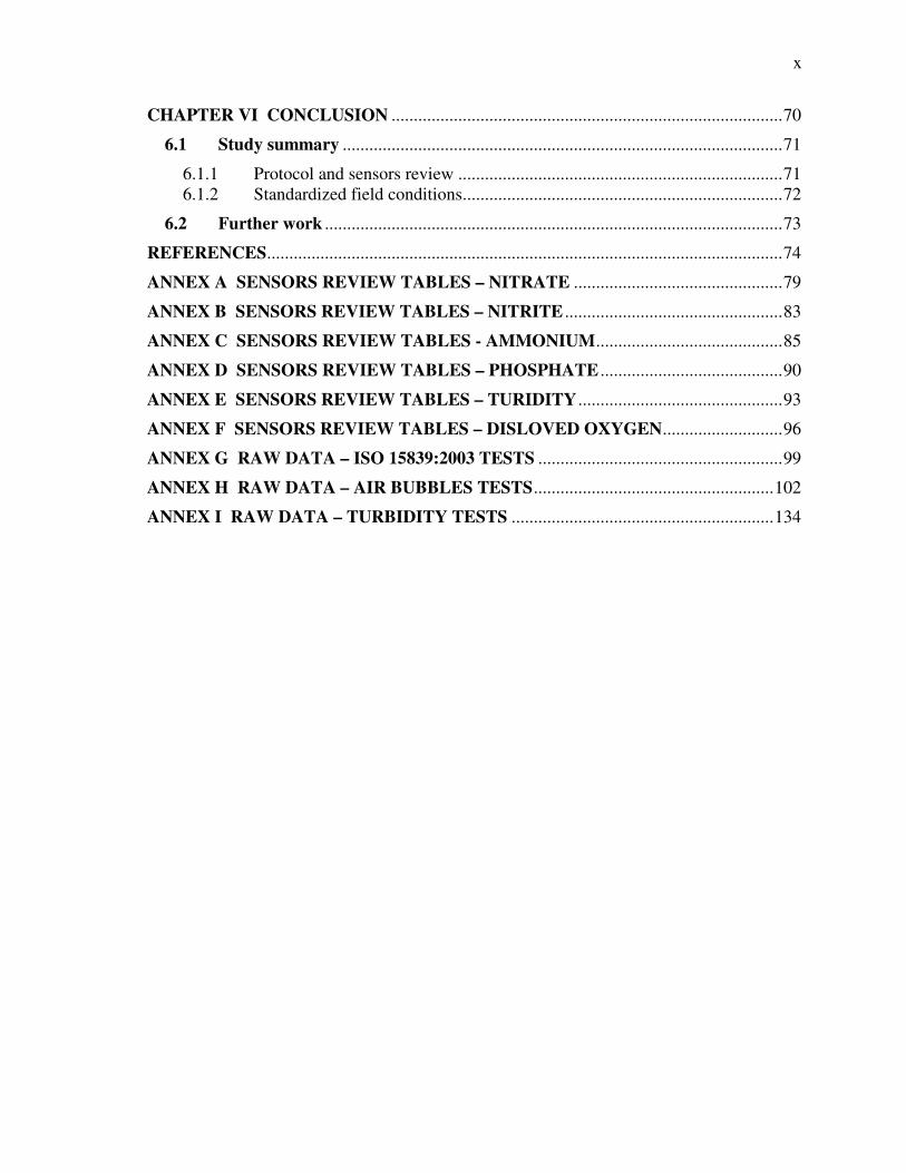
CHAPTER VI CONCLUSION ........................................................................................70
6.1 Study summary ...................................................................................................71
6.1.1 Protocol and sensors review .........................................................................71 6.1.2 Standardized field conditions........................................................................72
6.2 Further work .......................................................................................................73
REFERENCES....................................................................................................................74
ANNEX A SENSORS REVIEW TABLES – NITRATE ...............................................79
ANNEX B SENSORS REVIEW TABLES – NITRITE .................................................83
ANNEX C SENSORS REVIEW TABLES - AMMONIUM..........................................85
ANNEX D SENSORS REVIEW TABLES – PHOSPHATE .........................................90
ANNEX E SENSORS REVIEW TABLES – TURIDITY ..............................................93
ANNEX F SENSORS REVIEW TABLES – DISLOVED OXYGEN...........................96
ANNEX G RAW DATA – ISO 15839:2003 TESTS .......................................................99
ANNEX H RAW DATA – AIR BUBBLES TESTS......................................................102
ANNEX I RAW DATA – TURBIDITY TESTS ...........................................................134
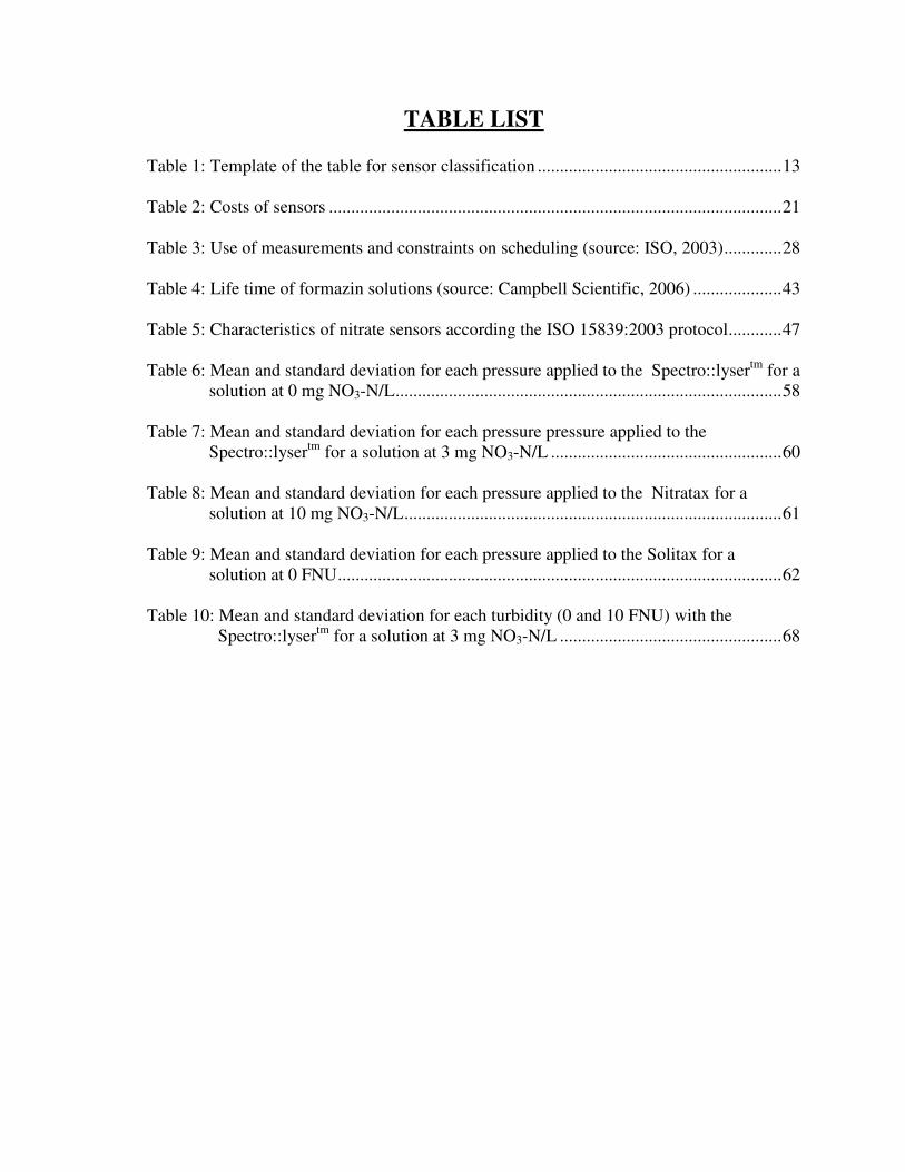
TABLE LIST Table 1: Template of the table for sensor classification .......................................................13 Table 2: Costs of sensors ......................................................................................................21 Table 3: Use of measurements and constraints on scheduling (source: ISO, 2003).............28 Table 4: Life time of formazin solutions (source: Campbell Scientific, 2006) ....................43 Table 5: Characteristics of nitrate sensors according the ISO 15839:2003 protocol............47 Table 6: Mean and standard deviation for each pressure applied to the Spectro::lysertm for a solution at 0 mg NO3-N/L.......................................................................................58 Table 7: Mean and standard deviation for each pressure pressure applied to the Spectro::lysertm for a solution at 3 mg NO3-N/L ....................................................60 Table 8: Mean and standard deviation for each pressure applied to the Nitratax for a solution at 10 mg NO3-N/L.....................................................................................61 Table 9: Mean and standard deviation for each pressure applied to the Solitax for a solution at 0 FNU....................................................................................................62 Table 10: Mean and standard deviation for each turbidity (0 and 10 FNU) with the Spectro::lysertm for a solution at 3 mg NO3-N/L ..................................................68
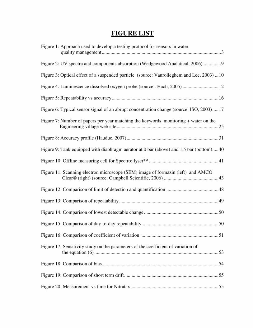
FIGURE LIST
Figure 1: Approach used to develop a testing protocol for sensors in water quality management................................................................................................3 Figure 2: UV spectra and components absorption (Wedgewood Analatical, 2006) ..............9 Figure 3: Optical effect of a suspended particle (source: Vanrolleghem and Lee, 2003) ...10 Figure 4: Luminescence dissolved oxygen probe (source : Hach, 2005) .............................12 Figure 5: Repeatability vs accuracy......................................................................................16 Figure 6: Typical sensor signal of an abrupt concentration change (source: ISO, 2003).....17 Figure 7: Number of papers per year matching the keywords monitoring + water on the Engineering village web site..................................................................................25 Figure 8: Accuracy profile (Hauduc, 2007)..........................................................................31 Figure 9: Tank equipped with diaphragm aerator at 0 bar (above) and 1.5 bar (bottom).....40 Figure 10: Offline measuring cell for Spectro::lyser™ ........................................................41 Figure 11: Scanning electron microscope (SEM) image of formazin (left) and AMCO Clear® (right) (source: Campbell Scientific, 2006) ............................................43 Figure 12: Comparison of limit of detection and quantification ..........................................48 Figure 13: Comparison of repeatability ................................................................................49 Figure 14: Comparison of lowest detectable change ............................................................50 Figure 15: Comparison of day-to-day repeatability..............................................................50 Figure 16: Comparison of coefficient of variation ...............................................................51 Figure 17: Sensitivity study on the parameters of the coefficient of variation of the equation (6) ....................................................................................................53 Figure 18: Comparison of bias..............................................................................................54 Figure 19: Comparison of short term drift............................................................................55 Figure 20: Measurement vs time for Nitratax.......................................................................55
xiii
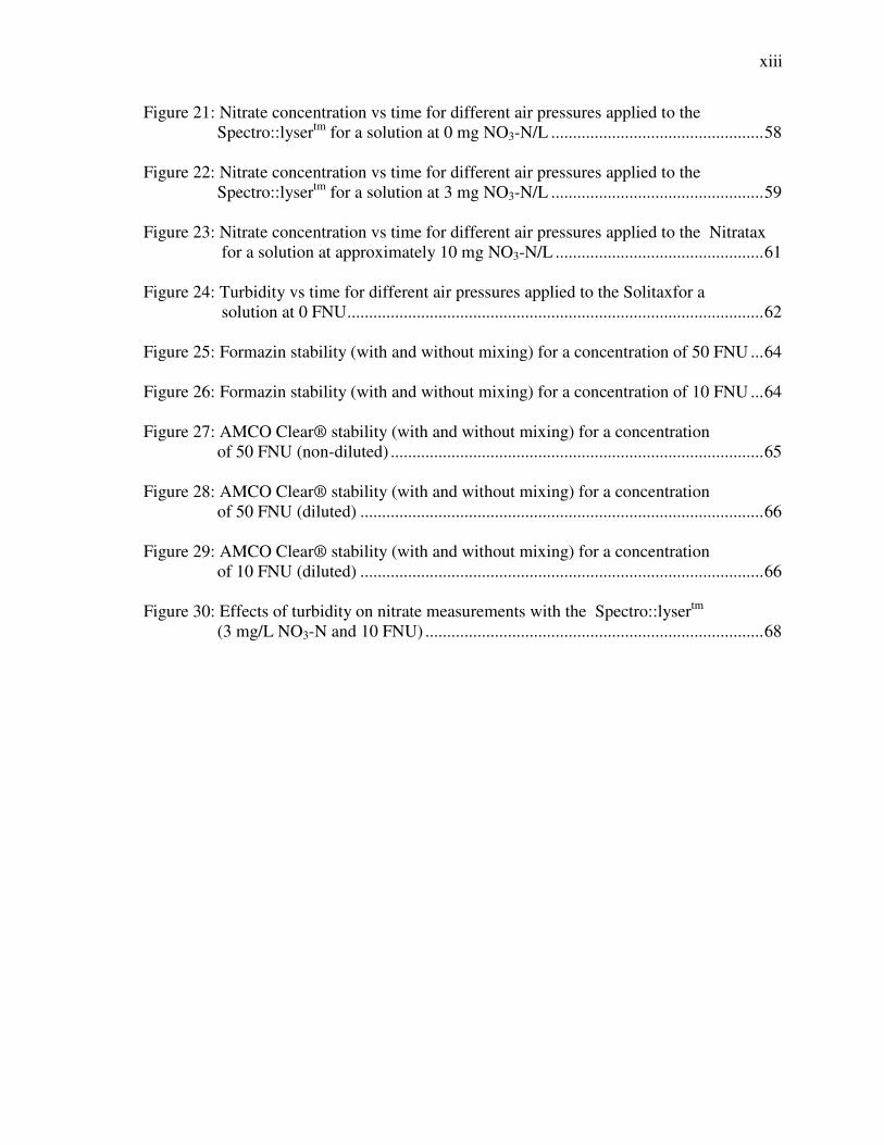
Figure 21: Nitrate concentration vs time for different air pressures applied to the Spectro::lysertm for a solution at 0 mg NO3-N/L .................................................58 Figure 22: Nitrate concentration vs time for different air pressures applied to the Spectro::lysertm for a solution at 3 mg NO3-N/L .................................................59 Figure 23: Nitrate concentration vs time for different air pressures applied to the Nitratax for a solution at approximately 10 mg NO3-N/L ................................................61 Figure 24: Turbidity vs time for different air pressures applied to the Solitaxfor a solution at 0 FNU................................................................................................62 Figure 25: Formazin stability (with and without mixing) for a concentration of 50 FNU ...64 Figure 26: Formazin stability (with and without mixing) for a concentration of 10 FNU ...64 Figure 27: AMCO Clear® stability (with and without mixing) for a concentration of 50 FNU (non-diluted) ......................................................................................65 Figure 28: AMCO Clear® stability (with and without mixing) for a concentration of 50 FNU (diluted) .............................................................................................66 Figure 29: AMCO Clear® stability (with and without mixing) for a concentration of 10 FNU (diluted) .............................................................................................66 Figure 30: Effects of turbidity on nitrate measurements with the Spectro::lysertm (3 mg/L NO3-N and 10 FNU) ..............................................................................68

CHAPTER I
GENERAL INTRODUCTION
2
1.1 Problem statement
The number of sensors on the market in water quality is large. For each component,
except for some of them, there are different measuring methods, different configurations,
and different manufacturers. All those factors are responsible for the multitude of sensors
available to end-users. However, how can end-users make an informed choice among the
available sensors? Which tools are available to characterise sensors? Are they sufficient?
How can they be improved?
1.2 Structure of the work done
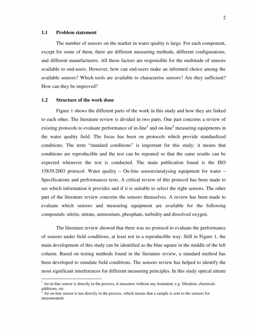
Figure 1 shows the different parts of the work in this study and how they are linked
to each other. The literature review is divided in two parts. One part concerns a review of
existing protocols to evaluate performance of in-line1 and on-line2 measuring equipments in
the water quality field. The focus has been on protocols which provide standardized
conditions. The term “standard conditions” is important for this study: it means that
conditions are reproducible and the test can be repeated so that the same results can be
expected whenever the test is conducted. The main publication found is the ISO
15839:2003 protocol: Water quality – On-line sensors/analysing equipment for water –
Specifications and performances tests. A critical review of this protocol has been made to
see which information it provides and if it is suitable to select the right sensors. The other
part of the literature review concerns the sensors themselves. A review has been made to
evaluate which sensors and measuring equipment are available for the following
compounds: nitrite, nitrate, ammonium, phosphate, turbidity and dissolved oxygen.
The literature review showed that there was no protocol to evaluate the performance
of sensors under field conditions, at least not in a reproducible way. Still in Figure 1, the
main development of this study can be identified as the blue square in the middle of the left
column. Based on testing methods found in the literature review, a standard method has
been developed to simulate field conditions. The sensors review has helped to identify the
most significant interferences for different measuring principles. In this study optical nitrate
1 An in-line sensor is directly in the process, it measures without any treatment, e.g. filtration, chemicals additions, etc. 2 An on-line sensor is not directly in the process, which means that a sample is sent to the sensors for measurement.
3
sensors were tested and the selected interferences were turbidity and air bubbles (typically
present in aerated reactors in wastewater treatment plants). The literature and sensors
review and the new protocol for standardised field conditions will be integrated into a new
protocol. This protocol will come with a piece of software, which is a Matlab script, that
will give end-users all sensor performance data. The protocol will also include a cost
calculation tool. This protocol will finally lead end-users to make the right choice for their
specific applications.
Figure 1: Approach used to develop a testing protocol for sensors in water quality management
4
1.3 Goals of this study
The first objective of this study is to characterise sensors according to available
protocols to evaluate the performance of on-line and in-line sensors in the water quality
field and to determine if the results coming out of those tests are meaningful and useful to
select the right sensor for a specific application.
The second objective is to develop a protocol in which field conditions are
reproduced to mimic those under which sensors are exposed while they are measuring and
evaluate the effects of the disturbances sensors are exposed to. It is important that those
conditions are not time nor site specific. This new protocol will be appended to existing
protocols to develop a tool that will help end-users to select the right sensors for their
application.
1.4 Thesis Outline
This master’s thesis is divided in six chapters. The first one presents a general
introduction of the topic, the context, the problem statement and the objectives of this work.
The second and third chapters present the literature review with chapter two presenting a
sensors review and chapter three presenting the protocol review. The fourth chapter
describes the materials and methods used for this study. Chapter five presents the results
obtained and their analysis and finally, chapter six provides an overview of the work done
and the conclusion.
CHAPTER II
REVIEW OF ON-LINE WATER QUALITY SENSORS
6
2.1 Review of on-line water quality sensors
Before knowing how to evaluate, test or use sensors it is essential to know the
sensors themselves, their measuring principle, the conditions for their operation, etc. Via
the Google web search engine3, companies providing measuring devices for water have
been identified and selected. There is a multitude of compounds that can be measured and
since the aim was not to cover all of them, a selection was made. The variables most used
in river water quality monitoring and in wastewater treatment plants (WWTP) have been
selected, i.e. dissolved oxygen (DO), nutrients (ammonium, nitrate, nitrite, phosphate) and
turbidity.
Recently, in 2005, the International Water Association (IWA) has published a book
covering this topic, Instrumentation, Control and Automation in Wastewater Systems. This
book covers sensors more widely, but one chapter is more important for the topic of this
work, Online Sensors/Analysers at Wastewater Treatment Plants. There is a discussion
about which kind of measuring methods are available to measure the most common
parameters, i.e. flow, level, pressure, temperature, pH, redox potential, conductivity, DO,
turbidity, sludge concentration, nutrients, total P and N, biological oxygen demand (BOD),
chemical oxygen demand (COD) and total organic carbon (TOC). There is also a review of
principal manufacturers of sensors/analysers. In this field the technological development is
quite fast and that is why this sensors review has been made.
2.2 Measuring principles
The aim was to compile information collected in a way that can be easily found and
that can be used to compare sensors among each other. So, one table has been made for
each selected compound. In the heading of the table, one section has been made for each
measuring principle. There are some descriptions of different measuring principles and a
review of measuring principles has already been made (Vanrolleghem and Lee, 2003),
while a synthesis of useful information has been added for this study.
3 Keywords used were the compound desired and sensor, e.g. nitrate sensor
7
2.2.1 Gas sensitive electrode
This method is used to measure ammonium. By increasing the pH to 11, all
ammonium ions (NH4+) are transformed in ammonia gas (NH3). The gas selective electrode
is equipped with a membrane which has the property to let pass the desired component, in
this case ammonia. This method requires an ex-situ installation; it means that pumping is
needed and in some cases a filtration unit as well. The reaction can be done in batch or in
continuous mode (Wacheux et al., 1996). Typically, the response time of the whole
measuring chain is 15 min (Thomsen and Nielsen, 1992). Measuring problems occurring
during operation could be caused by clogging and hydroxide poisoning of the electrode
(Aspegren et al., 1993), electrode drift (Patry and Takács, 1995) and gas bubble retention
under the electrode tip (Andersen and Wagner, 1990).
2.2.2 Ion sensitive electrode
The method is based on the same principle as the gas sensitive electrode, i.e. the
electrode has a membrane which lets pass the desired component. Such sensors are based
on the potentiometric measurement principle (Cammann, 1979). However, in this case it is
a direct measurement, i.e. the compound is directly measured and not a product of a
chemical reaction. The result is a low consumption of chemicals and a short response time
(Thomsen and Nielsen, 1992; Barnard and Crowther, 1993). For the time being, this
principle is used for the measurement of ammonium and nitrate (NO3-). This kind of
sensors can be used directly in the process, river, lake, etc. It is an in-situ sensor. As for the
gas sensitive electrodes, the ion sensitive electrodes (ISE) can be contaminated (Wacheux
et al., 1993; Sikow and Pursiainen, 1995). ISE can also suffer from electrode drift
(Wacheux et al., 1993). HCO3- (Sikow and Pursiainen, 1995), Cl- (APHA, 1992), bromide
(Rieger et al., 2002; Winkler et al., 2004) and iodine (Winkler et al., 2004) are interfering
ions for nitrate. The nitrate electrode drift can be fixed by automatic calibration (Sin et al.,
2003; Petersen et al., 2002). Amines, mercury and silver interfere in the ammonia
measurement (APHA, 2005) as well as potassium and sodium (Rieger et al., 2002; Winkler
et al., 2004).
8
2.2.3 Colorimetry
Usually colorimetric methods are implemented as ex-situ analyses (some models are
based on the same principle but are directly immerged in the medium). A known volume is
pumped through a filtering unit, and then the sample is brought in a small reactor.
Chemicals are added to react with the component to measure. The reaction could be done
both in batch or in a continuous flow (Wacheux et al., 1996). The reaction generates a
coloured component. With an optical cell, the absorbance or transmittance is measured and
this value is directly related to the component concentration. The principle is used for
nutrients, i.e. phosphate (PO43-), nitrate, ammonium and nitrite (NO2
-). The reagent
consumption is higher with such analysers (Thomsen and Nielsen, 1992) and the response
time with batch reactors is longer than with electrodes. Also, measurements are sensitive to
temperature variations (Wacheux et al., 1996) and are generally less reliable than ISE
(Harremoës et al., 1993).
2.2.4 UV-absorbance
A lot of components present in wastewater matrix absorb UV light. UV-absorbance,
as the other optical methods, has the advantage of being inexpensive, not requiring reagents
or sample preparation (Vanrolleghem and Lee, 2003). The principle is known and used for
more than fifty years (Dobbs et al., 1972), but in the last decade optical fibre technology
development has enabled remote and multi-point measurement (MacCraith et al., 1993).
This method is using a source of light in the UV spectral range from 190 nm to 720 nm.
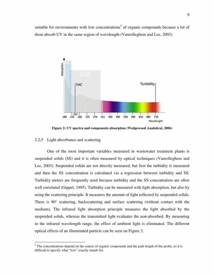
Figure 2 shows for which wavelength nitrates, chemical oxygen demand (COD)4, turbidity
and spectral absorption coefficient at 254 nm (SAC254) generate absorption. SAC254 is an
accepted standard parameter but it has limited dynamic range and usually underestimates
the organic load in wastewater (STIP, 2006). The method is advantageous for its low
maintenance need (Thomsen and Nielsen, 1992; Sikow and Pursiainen, 1995) and short
response time, approximately 10 seconds (Wacheux et al., 1993). UV-absorbance is
4 For nitrates and COD, the concentrations are estimated via the integration of the absorbance curve of the region where the compound absorbs light. A regression curve is made between lab analyses of samples and the selected absorbances.
9
suitable for environments with low concentrations5 of organic compounds because a lot of
them absorb UV in the same region of wavelength (Vanrolleghem and Lee, 2003).
Figure 2: UV spectra and components absorption (Wedgewood Analatical, 2006)
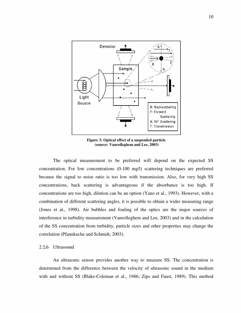
2.2.5 Light absorbance and scattering
One of the most important variables measured in wastewater treatment plants is
suspended solids (SS) and it is often measured by optical techniques (Vanrolleghem and
Lee, 2003). Suspended solids are not directly measured, but first the turbidity is measured
and then the SS concentration is calculated via a regression between turbidity and SS.
Turbidity meters are frequently used because turbidity and the SS concentration are often
well correlated (Gippel, 1995). Turbidity can be measured with light absorption, but also by
using the scattering principle. It measures the amount of light reflected by suspended solids.
There is 90° scattering, backscattering and surface scattering (without contact with the
medium). The infrared light absorption principle measures the light absorbed by the
suspended solids, whereas the transmitted light evaluates the non-absorbed. By measuring
in the infrared wavelength range, the effect of ambient light is eliminated. The different
optical effects of an illuminated particle can be seen on Figure 3.
5 The concentrations depend on the source of organic compounds and the path length of the probe, so it is difficult to specify what “low” exactly stands for.
10
Figure 3: Optical effect of a suspended particle
(source: Vanrolleghem and Lee, 2003) The optical measurement to be preferred will depend on the expected SS
concentration. For low concentrations (0-100 mg/l) scattering techniques are preferred
because the signal to noise ratio is too low with transmission. Also, for very high SS
concentrations, back scattering is advantageous if the absorbance is too high. If
concentrations are too high, dilution can be an option (Yano et al., 1993). However, with a
combination of different scattering angles, it is possible to obtain a wider measuring range
(Jones et al., 1998). Air bubbles and fouling of the optics are the major sources of
interference in turbidity measurement (Vanrolleghem and Lee, 2003) and in the calculation
of the SS concentration from turbidity, particle sizes and other properties may change the
correlation (Pfannkuche and Schmidt, 2003).
2.2.6 Ultrasound
An ultrasonic sensor provides another way to measure SS. The concentration is
determined from the difference between the velocity of ultrasonic sound in the medium
with and without SS (Blake-Coleman et al., 1986; Zips and Faust, 1989). This method
11
requires a SS-free reference, i.e. the sensor needs a calibration for each location (Olsson
and Nielsen, 1997).
2.2.7 Dielectric probe
To measure viable biomass, the dielectric properties of intact cells have been used
(Davey et al., 1993; Spierings, 1998; November and Van Impe, 2001). When an electric
field is applied to a suspension of cells in an aqueous solution, it results in a movement of
ions in the solution and within the cells. Then a charge separation or a polarization across
the cell membrane is created. The measurement of the resulting capacitance can be used to
monitor the biomass concentration (Davey et al., 1993). This method is advantageous to
measure only metabolically active biomass, but a change of the water capacitance or of the
cell membrane structure, composition and permeability can interfere (Vanrolleghem and
Lee, 2003).
2.2.8 Electrochemistry
Electrochemical measuring principles have been identified during the sensors
review for dissolved oxygen (DO). The electrochemical principle uses the oxidation by
DO. Oxygen is reduced to hydroxide ions (OH-) on the gold cathode. On the counter
electrode, DO oxidizes silver ions (Ag+) that adsorb on a silver bromide layer (AgBr). The
associated release of electrons from the gold cathode and the acceptance of electrons at the
counter electrode result in a current which, under constant conditions, is proportional to the
concentration of oxygen in the medium (Endress+Hauser, 2006a). Some sensors have an
exposed electrode while others are covered by a membrane which is DO selective.
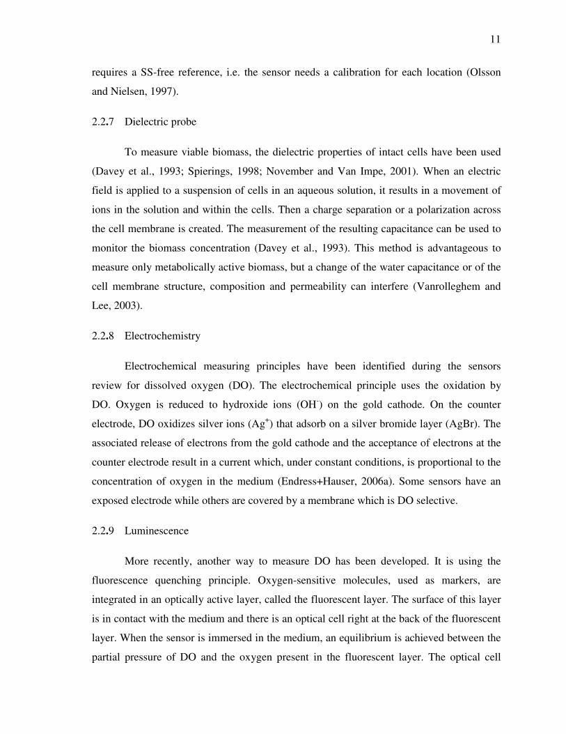
2.2.9 Luminescence
More recently, another way to measure DO has been developed. It is using the
fluorescence quenching principle. Oxygen-sensitive molecules, used as markers, are
integrated in an optically active layer, called the fluorescent layer. The surface of this layer
is in contact with the medium and there is an optical cell right at the back of the fluorescent
layer. When the sensor is immersed in the medium, an equilibrium is achieved between the
partial pressure of DO and the oxygen present in the fluorescent layer. The optical cell
12
emits green light pulses to the layer. The oxygen sensitive markers respond with a red light
fluorescence that is captured by the photo-sensitive diode. The duration and intensity of the
response signals of the markers depend directly on the oxygen content or partial pressure
(Endress+Hauser, 2006b). Different components of this kind of sensor can be identified on
Figure 4.
Figure 4: Luminescence dissolved oxygen probe6 (source : Hach, 2005)
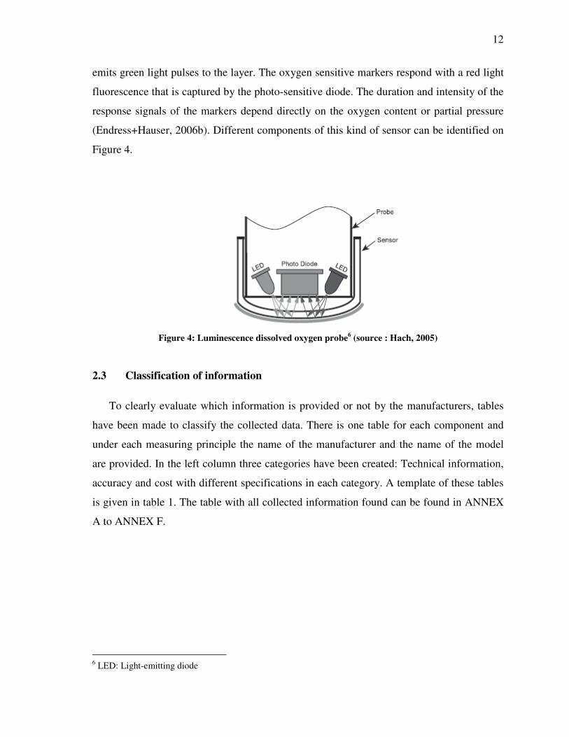
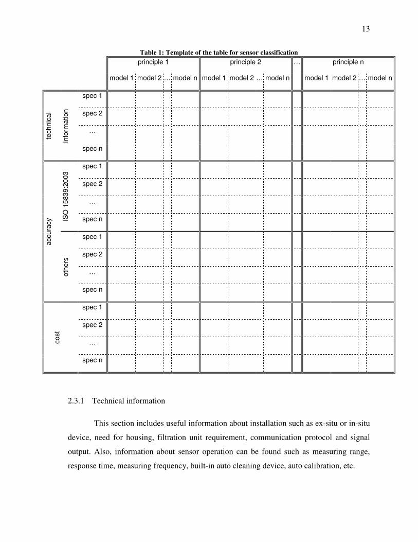
2.3 Classification of information
To clearly evaluate which information is provided or not by the manufacturers, tables
have been made to classify the collected data. There is one table for each component and
under each measuring principle the name of the manufacturer and the name of the model
are provided. In the left column three categories have been created: Technical information,
accuracy and cost with different specifications in each category. A template of these tables
is given in table 1. The table with all collected information found can be found in ANNEX
A to ANNEX F.
6 LED: Light-emitting diode
13
Table 1: Template of the table for sensor classification principle 1 principle 2 … principle n
model 1 model 2 … model n model 1 model 2 … model n model 1 model 2 … model n
spec 1
spec 2
…
technic
al
info
rmation
spec n
spec 1
spec 2
…
ISO
15
839
:20
03
spec n
spec 1
spec 2
…
accura
cy
oth
ers
spec n
spec 1
spec 2
… cost
spec n
2.3.1 Technical information
This section includes useful information about installation such as ex-situ or in-situ
device, need for housing, filtration unit requirement, communication protocol and signal
output. Also, information about sensor operation can be found such as measuring range,
response time, measuring frequency, built-in auto cleaning device, auto calibration, etc.
14
2.3.2 Accuracy
Some companies use this term as precision, but the definition in the dictionary is
“the state of being exact” (Oxford Online Dictionary, 2005). As the definition implies, this
category includes evaluation criteria to determine data quality (see Table 1) . This category
has been divided in two sub-sections, the first one including all terms defined in the (ISO
15839, 2003) the description of which will be given below. The other sub-section includes
other information provided by the manufacturers but not defined by the ISO standard. The
definitions of the terms used in the tables are taken from the ISO 15839:2003 standard:
2.3.2.1 Prior definitions
Accepted reference value
Value that serves as an agreed reference value for comparison, and which is derived as:
a) an assigned or certified value based on experimental work of some national or
international organisation;
b) a consensus or certified value based on collaborative experimental work;
c) a theoretical or established value based on scientific principles;
d) when a), b) and c) are not available, the expectation of the (measurable) quantity,
i.e. the mean of a number of measurements.
Day-to-day repeatability conditions
Conditions whereby independent test results are obtained with the same method on
identical test items in the same laboratory by the same operator using the same equipment
and reagents over several days.
15
Determinand
Property/substance that is required to be measured and to be reflected by/present in a
calibration solution.
Measurement chain
Set of instruments and actions that covers all steps involved in measuring a determinand,
including the on-line sensor/analysing equipment, sampling and pre-treatment,
transportation and storage of the sample.
Measuring range
Range between the lowest and the highest determinand value that a sensor/analysing
equipment can measure.
Repeatability conditions
Conditions where independent test results are obtained with the same method on identical
test items in the same laboratory by the same operator using the same equipment and
reagents within shot intervals of time (e.g. one day)
Working range
Range between the lowest and the highest determinand value for which tests to determine
precision and bias have been carried out.
2.3.2.2 Sensor characteristics definitions
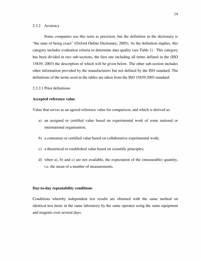
Precision
The closeness of agreement between independently measured values obtained under
stipulated conditions (see Figure 5).
16
Figure 5: Repeatability vs accuracy
Repeatability
Precision under repeatability conditions. It is equal to the standard deviation (sxo) of 6
measurements carried out at 20% and 80% of the measuring range, see and Figure 5
equation (1).
2
1
1( )
N
xo i
i
s x xN =
= −∑ (1)
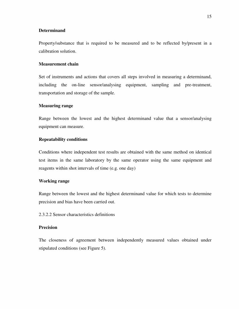
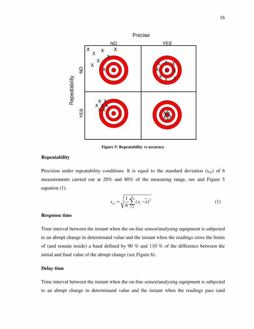
Response time
Time interval between the instant when the on-line sensor/analysing equipment is subjected
to an abrupt change in determinand value and the instant when the readings cross the limits
of (and remain inside) a band defined by 90 % and 110 % of the difference between the
initial and final value of the abrupt change (see Figure 6).
Delay time
Time interval between the instant when the on-line sensor/analysing equipment is subjected
to an abrupt change in determinand value and the instant when the readings pass (and
17
remain beyond) 10 % of the difference between the initial and final value of the abrupt
change (see Figure 6).
Rise time
Difference between the response time and the delay time when the abrupt change in
determinand value is positive (see Figure 6).
Figure 6: Typical sensor signal of an abrupt concentration change (source: ISO, 2003)
18
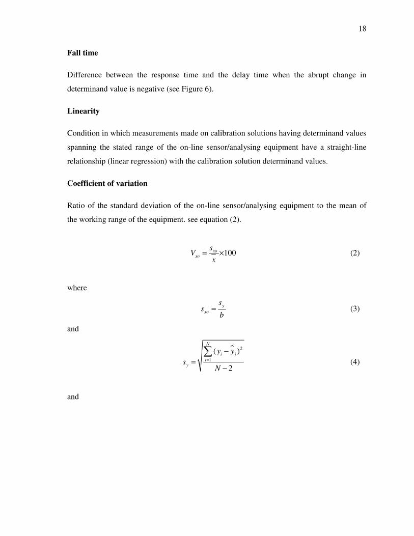
Fall time
Difference between the response time and the delay time when the abrupt change in
determinand value is negative (see Figure 6).
Linearity
Condition in which measurements made on calibration solutions having determinand values
spanning the stated range of the on-line sensor/analysing equipment have a straight-line
relationship (linear regression) with the calibration solution determinand values.
Coefficient of variation
Ratio of the standard deviation of the on-line sensor/analysing equipment to the mean of
the working range of the equipment. see equation (2).
100xoxo
sV
x= × (2)
where
y
xo
ss
b= (3)
and
� 2
1
( )
2
N
i i
iy
y y
sN
=
−
=−
∑ (4)
and
19
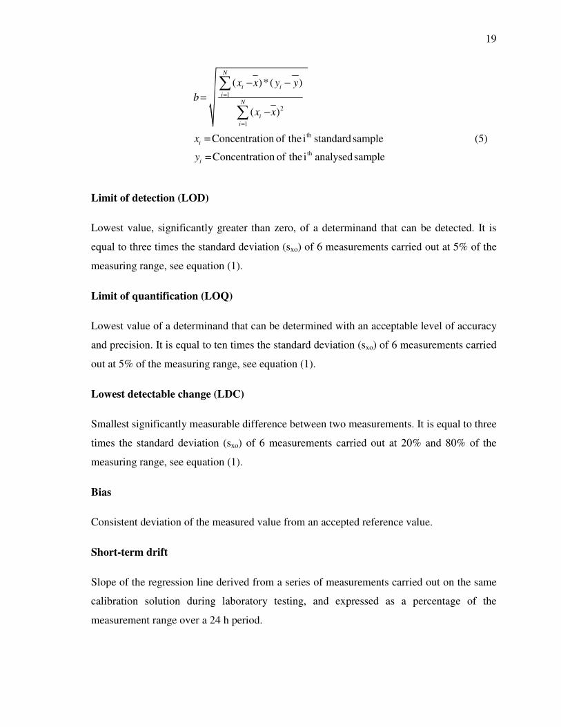
1
2
1
th
th
( )*( )
( )
Concentration of the i standardsample
Concentration of the i analysedsample
N
i i
i
N
i
i
i
i
x x y y
b
x x
x
y
=
=
− −
=
−
=
=
∑
∑
(5)
Limit of detection (LOD)
Lowest value, significantly greater than zero, of a determinand that can be detected. It is
equal to three times the standard deviation (sxo) of 6 measurements carried out at 5% of the
measuring range, see equation (1).
Limit of quantification (LOQ)
Lowest value of a determinand that can be determined with an acceptable level of accuracy
and precision. It is equal to ten times the standard deviation (sxo) of 6 measurements carried
out at 5% of the measuring range, see equation (1).
Lowest detectable change (LDC)
Smallest significantly measurable difference between two measurements. It is equal to three
times the standard deviation (sxo) of 6 measurements carried out at 20% and 80% of the
measuring range, see equation (1).
Bias
Consistent deviation of the measured value from an accepted reference value.
Short-term drift
Slope of the regression line derived from a series of measurements carried out on the same
calibration solution during laboratory testing, and expressed as a percentage of the
measurement range over a 24 h period.
20
Long term drift
Slope of the regression line derived from a series of differences between reference and
measurement values obtained during field testing, expressed as a percentage of the working
range over a 24 h period.
Day-to-day repeatability
Precision under day-to-day repeatability conditions. It is equal to ten times the standard
deviation (sxo) of 6 measurements carried out at 35% and 65% of the measuring range, see
equation (1).
Memory effect
Temporary or permanent dependence of readings on one or several previous values of the
determinand.
Interferences
Undesired output signal caused by a property(ies)/substance(s) other than the one being
measured.
Availability
Percentage of the full measurement period during which the measurement chain is available
for making measurements.
Up-time
Percentage of a full measurement period during which the measurement chain is actually
measuring during field testing.
21
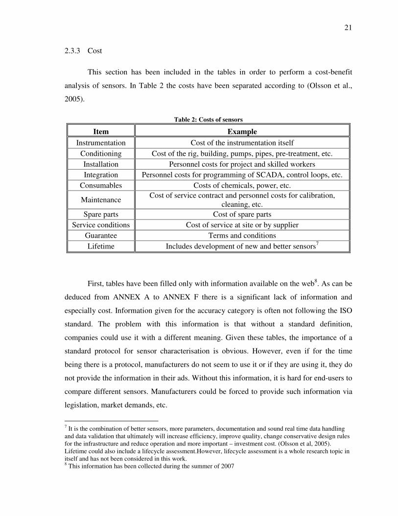
2.3.3 Cost
This section has been included in the tables in order to perform a cost-benefit
analysis of sensors. In Table 2 the costs have been separated according to (Olsson et al.,
2005).
Table 2: Costs of sensors
Item Example
Instrumentation Cost of the instrumentation itself Conditioning Cost of the rig, building, pumps, pipes, pre-treatment, etc. Installation Personnel costs for project and skilled workers Integration Personnel costs for programming of SCADA, control loops, etc.
Consumables Costs of chemicals, power, etc.
Maintenance Cost of service contract and personnel costs for calibration,
cleaning, etc. Spare parts Cost of spare parts
Service conditions Cost of service at site or by supplier Guarantee Terms and conditions Lifetime Includes development of new and better sensors7
First, tables have been filled only with information available on the web8. As can be
deduced from ANNEX A to ANNEX F there is a significant lack of information and
especially cost. Information given for the accuracy category is often not following the ISO
standard. The problem with this information is that without a standard definition,
companies could use it with a different meaning. Given these tables, the importance of a
standard protocol for sensor characterisation is obvious. However, even if for the time
being there is a protocol, manufacturers do not seem to use it or if they are using it, they do
not provide the information in their ads. Without this information, it is hard for end-users to
compare different sensors. Manufacturers could be forced to provide such information via
legislation, market demands, etc.
7 It is the combination of better sensors, more parameters, documentation and sound real time data handling and data validation that ultimately will increase efficiency, improve quality, change conservative design rules for the infrastructure and reduce operation and more important – investment cost. (Olsson et al, 2005). Lifetime could also include a lifecycle assessment.However, lifecycle assessment is a whole research topic in itself and has not been considered in this work. 8 This information has been collected during the summer of 2007
22
2.4 Conclusion
By doing the sensors review and the classification of information, it has been
observed that companies fail to provide information according the ISO 15839:2003
protocol. Moreover, definitions of the ISO protocol are not followed by companies in their
sensors specifications. Why do companies fail to provide information according the ISO
protocol and are not following definitions? It may be because the ISO 15839 standard is
relatively new, dating from 2003. Maybe they did not have the time to implement it in their
procedure. Another reason could be that it is complicated to use this protocol. To
understand the underlying reasons for the observation that manufacturers do not supply the
ISO-standard sensors characterisation it may be useful to apply standards. That is why a
review of the ISO standard has to be made, first to see what is included and what is not.
The procedure will be applied with different nitrate sensors using the optical measuring
principle.
The sensors review has shown as well that there are a lot of different measuring
principles for each compound selected. Each of these measuring principles has its pros and
cons and they will perform differently in the laboratory and in the field. There is a need to
be informed on their behaviour under field conditions in order to evaluate the quality of
data that a sensor provides.
23
CHAPTER III
REVIEW OF SENSOR EVALUATION PROTOCOLS
24
3.1 Literature review introduction
Monitoring is defined, in the dictionary, as the act of observing something and
sometimes keeping a record of it (Ultralingua Online Dictionary, 2008). In the scientific
literature more specific definitions of monitoring can be found, e.g.: To track the current
process operational state via the instrumentation (Olsson et al., 2005). In the water
discipline (wastewater, rivers, catchments, etc.) monitoring has become easier with the
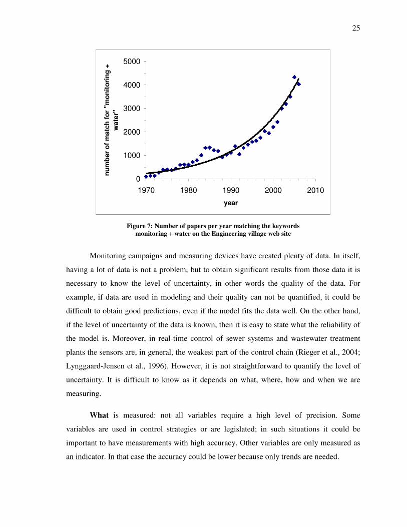
arrival of computers and new technologies. As can be seen in Figure 7, research activities
related to water monitoring have literally exploded since the seventies. It shows the number
of publications per year for the research on the Engineering Village web site for the
keywords “water” and “monitoring”. The exponential growth of papers published on this
topic each year can be observed. Moreover, with all issues in water quality and
management such as micro-pollutants, more restrictive legislation, energy efficiency, etc.,
the tendency will probably continue. New technologies have helped a lot in monitoring and
control: with sensors it is easier to monitor remote places, to measure different variables at
the same time and in control and automation it helps to meet regulatory requirements,
improve process performance and reliability, record data and create reports, save chemicals,
energy, labour and finally reduce risk and ensure a good night’s sleep (WEF, 2005).
25
0
1000
2000
3000
4000
5000
1970 1980 1990 2000 2010
year
nu
mb
er
of
matc
h f
or
''mo
nit
ori
ng
+
wate
r''
Figure 7: Number of papers per year matching the keywords
monitoring + water on the Engineering village web site
Monitoring campaigns and measuring devices have created plenty of data. In itself,
having a lot of data is not a problem, but to obtain significant results from those data it is
necessary to know the level of uncertainty, in other words the quality of the data. For
example, if data are used in modeling and their quality can not be quantified, it could be
difficult to obtain good predictions, even if the model fits the data well. On the other hand,
if the level of uncertainty of the data is known, then it is easy to state what the reliability of
the model is. Moreover, in real-time control of sewer systems and wastewater treatment
plants the sensors are, in general, the weakest part of the control chain (Rieger et al., 2004;
Lynggaard-Jensen et al., 1996). However, it is not straightforward to quantify the level of
uncertainty. It is difficult to know as it depends on what, where, how and when we are
measuring.
What is measured: not all variables require a high level of precision. Some
variables are used in control strategies or are legislated; in such situations it could be
important to have measurements with high accuracy. Other variables are only measured as
an indicator. In that case the accuracy could be lower because only trends are needed.
26
Where a variable is measured: depending on which variables are measured, there
may be plenty of other substances present in the matrix, which may interfere in the
measurement process. Moreover, the environmental conditions may also create
interferences. For example, if the phosphate concentration is measured with a photometric
analyser, the sample is pumped in a small reactor, and chemicals are added to generate a
reaction changing the solution’s color. The color intensity is subsequently measured with
an optical module, the color’s intensity being proportional to the phosphate concentration.
However, the reaction’s kinetics depend on sample temperature: if it is too cold the reaction
will be incomplete and the measurement could be wrong. Also, since it is an optical
measurement, suspended particles can interfere, and often it is therefore necessary to filter
the sample before heading it to the analyser. However, filtration creates others problems: if
the water is highly charged in total suspended solids (TSS), the filter will clog rapidly and
the maintenance interval will be short. Moreover, the filtration unit adds a time delay into
the measurement chain and this time delay is variable over time due to the clogging
phenomenon that is increasing. This is only one example, but there are a lot more aspects
to take into consideration.
How the variable is measured: for some substances there are only a few ways to
measure them, e.g. phosphate measurements: there is only the colorimetric principle, with
two different reactions depending on the concentration. For other compounds such as
ammonium there are at least five different methods (gas sensitive electrode, ion sensitive
electrode (ISE), colorimetric, titration, Fourier transform analysis of the absorption
spectrum of NH3 by adding sodium hydroxide). In such case, each method has is own
accuracy and each method reacts in a different way to other compounds present in the
matrix. It is important to know how to prepare, install and maintain such sensors to get the
maximum out of them.
When the variable is measured: this topic could have some similarities with the one
“where a variable is measured”. However, in this case the answer depends more on the
period of the day, week, year… and all changes occurring during those periods, e.g.
temperature, flow, concentration of the measured compound and the compounds of the
matrix, etc.
27
As mentioned earlier, evaluating data uncertainties is not straightforward. There is a
lot to consider to have a good idea regarding the uncertainties. Note that the same kind of
reasoning is necessary to choose the best sensors for end-users needs. However, when the
time comes to select and/or buy a measuring device, two main questions occur:
• What are the tools available to evaluate a sensor’s performance?
• On which basis should the sensors be compared to make the right choice?
To answer these questions, a sensors review was first made; and companies’
websites were consulted to know what kind of information they provide. Then a review of
available evaluation tools for sensors was conducted. Publications, books and information
provided by standard organisations (like ISO and ASTM International) were studied (1) to
know what is currently available, (2) to evaluate whether the information is sufficient,
useful and (3) to find out whether the protocols are user-friendly.
3.2 Laboratory conditions
3.2.1 ISO 15839:2003
The protocol ISO 15839:2003 “Water quality – On-line sensors/analysing
equipment for water – Specifications and performance tests” is the most complete one
found regarding sensor characterisation in water quality. It contains two main parts. The
first one concerns the determination of the performance characteristics in the laboratory: all
tests are to be conducted under standard laboratory conditions, i.e. solutions with pure
water and the measured component. The second part deals with performance characteristics
in the field (see below).
In the chapter of Automation of Wastewater Treatment Facilities (WEF, 2005) a
section is devoted to Characteristics of Online sensors. Everything in this section
corresponds to the ISO 15839:2003 standard, which is not surprising since one of the
authors of the book, Anders Lynggaard-Jensen, was member of the ISO committee. The
different definitions of the characteristics evaluated by the ISO standard are given, but
without adding new elements.
28
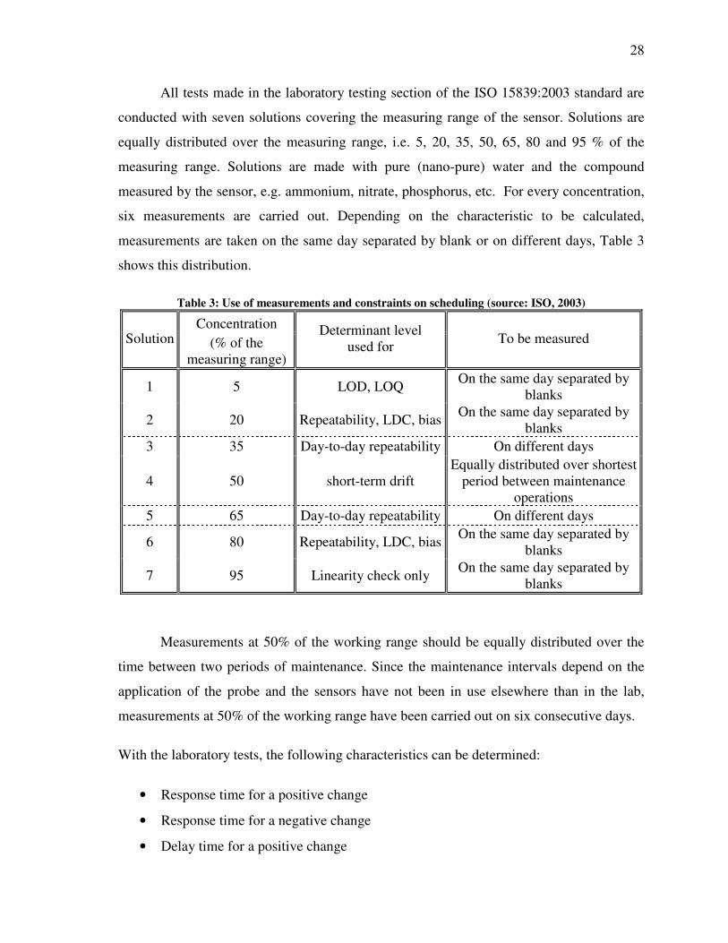
All tests made in the laboratory testing section of the ISO 15839:2003 standard are
conducted with seven solutions covering the measuring range of the sensor. Solutions are
equally distributed over the measuring range, i.e. 5, 20, 35, 50, 65, 80 and 95 % of the
measuring range. Solutions are made with pure (nano-pure) water and the compound
measured by the sensor, e.g. ammonium, nitrate, phosphorus, etc. For every concentration,
six measurements are carried out. Depending on the characteristic to be calculated,
measurements are taken on the same day separated by blank or on different days, Table 3
shows this distribution.
Table 3: Use of measurements and constraints on scheduling (source: ISO, 2003)
Concentration Solution (% of the
measuring range)
Determinant level used for
To be measured
1 5 LOD, LOQ On the same day separated by
blanks
2 20 Repeatability, LDC, bias On the same day separated by
blanks 3 35 Day-to-day repeatability On different days
4 50 short-term drift Equally distributed over shortest
period between maintenance operations
5 65 Day-to-day repeatability On different days
6 80 Repeatability, LDC, bias On the same day separated by
blanks
7 95 Linearity check only On the same day separated by
blanks
Measurements at 50% of the working range should be equally distributed over the
time between two periods of maintenance. Since the maintenance intervals depend on the
application of the probe and the sensors have not been in use elsewhere than in the lab,
measurements at 50% of the working range have been carried out on six consecutive days.
With the laboratory tests, the following characteristics can be determined:
• Response time for a positive change
• Response time for a negative change
• Delay time for a positive change
29
• Delay time for a negative change
• Rise time
• Fall time
• Linearity
• Coefficient of variation
• Limit of detection
• Limit of quantification
• Repeatability
• Lowest detectable change
• Bias
• Short-term drift
• Day-to-day repeatability
• Memory effect
• Interferences
• Environmental and operating conditions
This protocol provides a lot of information about testing under standard conditions.
There is almost nothing that can disturb the measurements; it is a good way to characterize
the maximum performance of sensors or to compare the performance of different
measuring devices. In fact, however, it is very rare to operate sensors under such
conditions. So, the sensors’ behaviour under field conditions can not be predicted with this
kind of procedure. As seen previously, manufacturers do not provide information resulting
from applying this protocol. The first part of this study will therefore be to go through the
protocol and do a critical review of it. Afterwards, it will be possible to come up with
suggestions, and bring some clarifications if needed.
3.2.2 Accuracy profile
Other techniques used to certify laboratory methods could be applied to this
particular topic as well. Accuracy profiles are used since a couple of years, mainly in the
pharmaceutical and food-processing industry (Hauduc, 2007). The principle of an accuracy
profile is based on a comparison of a limit of acceptance λ, which is representing the
30
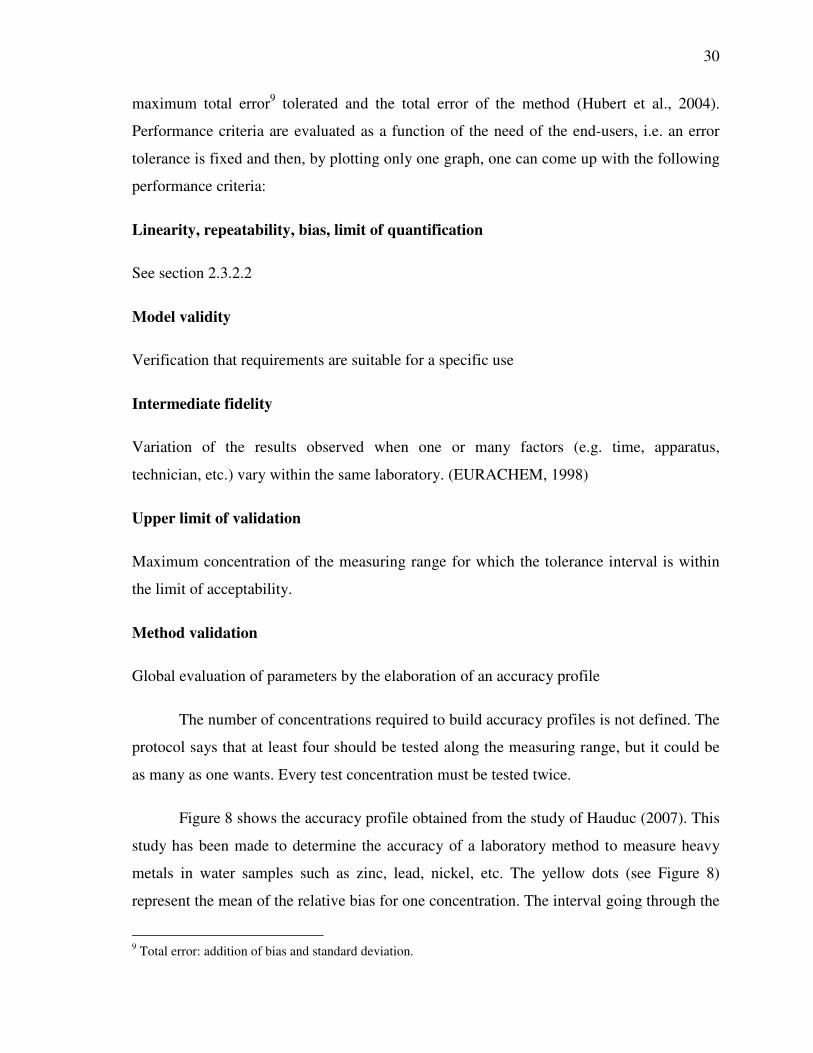
maximum total error9 tolerated and the total error of the method (Hubert et al., 2004).
Performance criteria are evaluated as a function of the need of the end-users, i.e. an error
tolerance is fixed and then, by plotting only one graph, one can come up with the following
performance criteria:
Linearity, repeatability, bias, limit of quantification
See section 2.3.2.2
Model validity
Verification that requirements are suitable for a specific use
Intermediate fidelity
Variation of the results observed when one or many factors (e.g. time, apparatus,
technician, etc.) vary within the same laboratory. (EURACHEM, 1998)
Upper limit of validation
Maximum concentration of the measuring range for which the tolerance interval is within
the limit of acceptability.
Method validation
Global evaluation of parameters by the elaboration of an accuracy profile
The number of concentrations required to build accuracy profiles is not defined. The
protocol says that at least four should be tested along the measuring range, but it could be
as many as one wants. Every test concentration must be tested twice.
Figure 8 shows the accuracy profile obtained from the study of Hauduc (2007). This
study has been made to determine the accuracy of a laboratory method to measure heavy
metals in water samples such as zinc, lead, nickel, etc. The yellow dots (see Figure 8)
represent the mean of the relative bias for one concentration. The interval going through the
9 Total error: addition of bias and standard deviation.
31
yellow dots represents the uncertainties of the reference measurements. Blue dotted lines
represent limits of tolerance (p). The tolerance p is calculated with standard the deviation of
repeatability and intermediate fidelity. For environmental analysis the tolerance must be
15% (Hubert et al., 2004). However, in the Directive Cadre sur l’Eau the tolerance on the
detection limit should be at least 50% (Hauduc, 2007). The intersection of the limit of
acceptability and of the limit of tolerance in the lower part of the measuring range
determines the limit of quantification. Between the intersection of the upper limit and the
lower limit, the higher value has to be considered as the limit of quantification.
-50%
-40%
-30%
-20%
-10%
0%
10%
20%
30%
40%
50%
0,0 10,0 20,0 30,0 40,0 50,0 60,0
Concentration (mg/l)
Bia
s
bias
low er limit of acceptability
upper limit of acceptability
low er limit of tolerance
upper limit of tolerance
LQ
Figure 8: Accuracy profile (Hauduc, 2007)
If the limit of acceptability would have crossed the limit of tolerance in the upper
part of the measuring range, there would have been an upper limit of validation. This means
in this case that the measuring method is valid from the limit of quantification until 50
mg/l, which is the highest concentration tested.
The direct value of the linearity can not be seen on the figure; however, it can be
estimated. For the best sensors all measurements are located on the line of 0% bias. A
sensor with a nearly perfect linearity but with measuring noise would have its
measurements equally distributed around the 0% bias line. If a sensor does not have a good
linearity, measurements will more often be one side of the 0% bias than the other.
32
This method demands more statistical knowledge to build the profiles, but with only
one figure, many performance criteria can be evaluated: bias, limit of quantification,
repeatability, limit of validation, linearity.
The accuracy profile methodology has not been tested in this work because the
sensors were no longer available when this methodology was found in the literature.
3.3 Field conditions
To overcome the problem of the lack of information on in field sensor performance,
there is a protocol included in the ISO 15839:2003 norm to evaluate sensor characteristics
during field operation. The main idea of this procedure is to expose sensors or analysers to
real conditions. Several ways are suggested: the measuring device could be installed
directly in the field (nearby the river, WWTP, lake, etc.). The problem with this set-up is
that there are dynamics imposed due to parameters such as flow rate, concentrations,
temperature, etc. Hence, when the moment comes to compare sensor data with real values
(laboratory analysis), because of the non-steady state conditions, one analysis has to be
made for each measurement taken by a sensor. Another approach consists of exposing
sensors to a grab sample from a real process. With a big enough sample, all tests could be
achieved with the same sample, but even in the absence of the outflow of the tank, there
still is a non-steady state for some compounds due to processes such as biodegradation,
stripping, etc. Hence, the problem could persist depending on what is measured. With this
part of the ISO protocol, the following characteristics could be evaluated:
• Response time for positive change
• Response time for negative change
• Delay time for positive change
• Delay time for negative change
• Rise time
• Fall time
• Bias based on (relative/absolute)
differences
• Long-term drift
• Availability
• Up-time
33
This procedure is useful to know how measuring devices will react under specific field
conditions. However, in the case one wants to make a comparison of sensor performances,
the only way to achieve it is to carry out the same procedure at exactly the same time and at
the same place. The part in the ISO 15839:2003 protocol concerning the determination of
the performance characteristics in the field is time and location specific. It means that, for
example, results collected on two different days from the same sensors mounted at the same
place can not be compared. Depending of what kind information is looked for, following
this procedure could be the right thing to do if the aim is to know how the sensors will react
in a specific process, river, lake, etc. However, when the goal is to compare the
performance of sensors or to state the performance of one sensor under field conditions this
procedure leads to non-significant results.
To have a procedure to test sensors that anybody could perform and always get the
same results, it has to be free of time and location influences, similar to the procedure for
determination of performance characteristics in the laboratory. This is called
reproducibility. Consequently, the ISO 15839:2003 protocol does not include an evaluation
tool for performance evaluation under reproducible field conditions. As can be seen in the
protocol, the standard and laboratory conditions are well documented but the field
condition testing is still an incompletely covered topic.
Moreover, this part of the protocol evaluates the performance of the whole
measuring chain without making a distinction between the different segments of the chain
(pump, filtering device, measuring cell, etc.). In other words, the measuring chain is
evaluated as a black box. If a bad measurement occurs, it will be difficult to point out
exactly where the problem is located.
From the above, it is clear there is a need to test sensors under standardized field
conditions. First, to easily compare sensors without the need of doing tests at the same time
and same location. Second, if it is possible to test field conditions in the lab, then it is easier
to isolate the different segments of the measuring chain, to perform spot checking and to
evaluate the effect of disturbances separately. With this knowledge, it will also be easier to
plan maintenance that is directly geared to the problematic segment.
34
3.4 Conclusions
To date the ISO 15839:2003 protocol is the most complete protocol to characterise
sensors for water quality. It provides a standard procedure to test sensors under laboratory
conditions. Nomenclature is defined and must be followed by manufacturers rather than
keep using their own nomenclature. This would help end-users to compare sensors from
different manufacturers by knowing the definitions of the terms used and by knowing as
well that manufacturers are following them.
On the other hand, information coming from laboratory testing does not give
indications of how the sensors will perform under field conditions. In the ISO 15839:2003
protocol a section about field conditions testing is given. This section is incomplete and
does not aim for reproducible results, the main reason being that tests are time and site
specific. It can help end-users to know how a sensor will perform in his specific
application, but at this step of characterisation, the sensor is already bought. In order to be
able to compare sensors’ performances under field conditions and help end-users to select
the right sensor, a standardized protocol for field conditions is needed.

CHAPTER IV
MATERIALS AND METHODS
36
The goal of this work is to characterize sensors under different conditions. As seen
before there are already some protocols available. So far the ISO 15839:2003 protocol is
the most complete and specific. For this work only the part concerning laboratory testing
will be conducted and described. Subsequently, the protocol to standardize field conditions,
i.e. the effect of air bubbles and turbidity, will be described.
4.1 Sensors tested
4.1.1 Spectro::lysertm from s::can
The Spectro::lysertm from the s::can company is a spectrometer covering the UV
spectrum from 190 to 390 nm. Different path lengths are available, depending on the
application. The one used in this work is a 35 mm path length, usually used for river water
quality monitoring. The sensor version is able to measure nitrate concentrations between 0
and 15 mg NO3-N/l. Auto-cleaning is performed with pressurized air. The probe is
provided with a global calibration, in this case the river calibration. It is possible to add, on
top of the global calibration, a local calibration or even a specific calibration (Rieger et al.,
2006). In this work, a local calibration has been performed with two points, at 20 and 80 %
of the working range, i.e. 3 and 12 mg NO3-N/l. The probe is connected to a computer via a
relay box; this box provides power to the probe and is processing the signal to a USB port
of the computer. s::can is also providing the data collection software. The one used is the
ana::pro V5.3e-2399. For continuous measurements, the measuring interval has been set to
the minimum, i.e. one minute. Tests with this probe have been conducted at Université
Laval.
4.1.2 Sensor A
Sensor A is a spectrometer using the same measuring principle as the s::can probe.
The measuring cell is not directly immersed in the water: with a small piston water is
pumped into a tube. The light source and the measuring cell are on each side of this cell.
With this kind of setup it is also possible to measure settling properties and perform water
quality measurements disturbed less by turbidity. The measuring range of sensor A is 0-20
mg/l of NO3-N. Every time the piston is moving in the tube, it is cleaning it. The calibration
37
used for the tests is the factory calibration. The only thing which has been added before
testing, is to set the zero with the water used to make the solutions. This probe was not used
in continuous measurement; only manual measurements were carried out. Tests were
conducted at the company’s laboratory.
4.1.3 Nitratax from Hach
The measuring principle of this probe is using two specific wavelengths, instead of
256 for the s::can Spectro::lysertm. The nitrate concentration is measured at 210 nm and a
turbidity correction is made with a measurement at 350 nm. The path length of the probe
used in the tests is 1mm allowing the probe to measure nitrate (as NO3-N) concentrations
from 0 to 100 mg/l. The auto-cleaning of lenses is made by a wiper. No additional
calibration has been made for the tests. The calibration used is the one made by the
technician of the company. The probe is connected to the SC100 controller that is
connected to a central server for data logging. During continuous measurements, the
measuring interval was set to the minimum value of 15 sec and during testing data filtering
was set to zero. Tests with this probe have been conducted at EAWAG in Zurich.
4.1.4 Sensor B-8mm and B-2mm
This sensor is still in development and is not yet on the market. It is also measuring
nitrate with the two wavelengths principle. Two path lengths are available for this model: 2
mm with a measuring range of 0 to 50 mg/l of NO3-N and 8 mm with a measuring range of
0 to 10 mg/l of NO3-N. Both configurations were tested in this work. The auto-cleaning of
the sensor is performed with pressurized air. The calibration used during the
experimentation was the factory calibration. The sensors were connected to the controller
provided by the company. Signal filtering and damping were set to zero. Since no
continuous measurements were carried out, the data logger was not configured. Tests were
conducted at the company’s laboratory.
38
4.1.5 Sensor C
Sensor C is also using the two wavelengths measuring principle. It can measure
concentrations from zero to 50 mg/l of nitrate as NO3-N. The auto-cleaning of lenses is
ensured by pressurized air. The calibration used during the experimentation was the factory
calibration. The probe was connected to the controller provided by the company. Data
filtering was set to zero. Since this sensor was not used for continuous measurements, the
data logger was not configured. Tests were conducted at the company’s laboratory.
4.1.6 Solitax from Hach
The Hach Solitax is a turbidity sensor. It is combining two different scattering
angles: 90° and 140°, allowing the sensor to measure turbidity from 0.001 to 4000 NTU.
The auto-cleaning of the lens is made by a wiper. The calibration used during the
experiments was the factory calibration. The sensor was connected to a Hach SC1000
controller, and the controller was connected to a computer to download the log files.
During continuous experimentation, the measurement frequency was set to the minimum,
i.e. 5 seconds. Tests were conducted at Université Laval.
4.2 ISO 15839:2003 – Laboratory testing
All sensor testing was conducted according to the ISO 15839:2003 protocol, see
section 3.2.1. Diluted solutions have been prepared from a high concentrate solution (1000
mg/l as NO3-N). Dilutions have been made with micropipettes and concentrations have
been double-checked with Hach test kits.
4.3 Standardised field conditions protocol
In this part of the work, the aim was to reproduce, in the laboratory, interferences
that can be found in the field. As mentioned previously, so far there is no methodology to
evaluate the effects of a single disturbance on the measurements. It has always been a
combination of effects. Therefore, a methodology has been developed to isolate
disturbances and quantify their effects on the measurements. The methodology has been
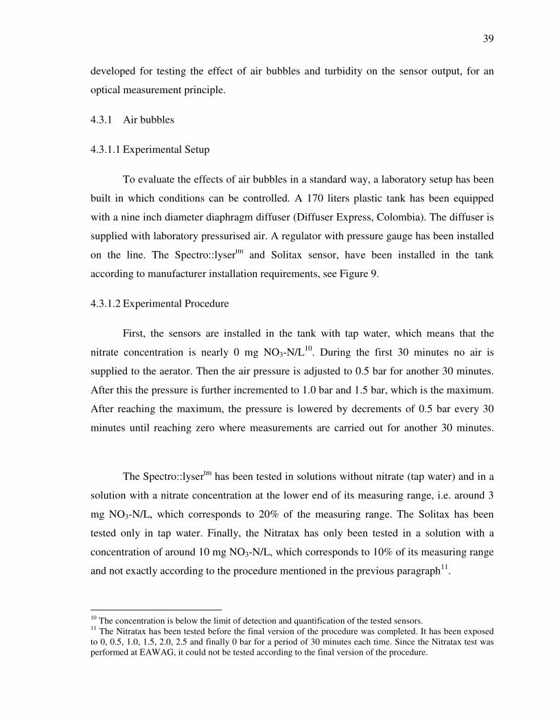
39
developed for testing the effect of air bubbles and turbidity on the sensor output, for an
optical measurement principle.
4.3.1 Air bubbles
4.3.1.1 Experimental Setup
To evaluate the effects of air bubbles in a standard way, a laboratory setup has been
built in which conditions can be controlled. A 170 liters plastic tank has been equipped
with a nine inch diameter diaphragm diffuser (Diffuser Express, Colombia). The diffuser is
supplied with laboratory pressurised air. A regulator with pressure gauge has been installed
on the line. The Spectro::lysertm and Solitax sensor, have been installed in the tank
according to manufacturer installation requirements, see Figure 9.
4.3.1.2 Experimental Procedure
First, the sensors are installed in the tank with tap water, which means that the
nitrate concentration is nearly 0 mg NO3-N/L10. During the first 30 minutes no air is
supplied to the aerator. Then the air pressure is adjusted to 0.5 bar for another 30 minutes.
After this the pressure is further incremented to 1.0 bar and 1.5 bar, which is the maximum.
After reaching the maximum, the pressure is lowered by decrements of 0.5 bar every 30
minutes until reaching zero where measurements are carried out for another 30 minutes.
The Spectro::lysertm has been tested in solutions without nitrate (tap water) and in a
solution with a nitrate concentration at the lower end of its measuring range, i.e. around 3
mg NO3-N/L, which corresponds to 20% of the measuring range. The Solitax has been
tested only in tap water. Finally, the Nitratax has only been tested in a solution with a
concentration of around 10 mg NO3-N/L, which corresponds to 10% of its measuring range
and not exactly according to the procedure mentioned in the previous paragraph11.
10 The concentration is below the limit of detection and quantification of the tested sensors. 11 The Nitratax has been tested before the final version of the procedure was completed. It has been exposed to 0, 0.5, 1.0, 1.5, 2.0, 2.5 and finally 0 bar for a period of 30 minutes each time. Since the Nitratax test was performed at EAWAG, it could not be tested according to the final version of the procedure.
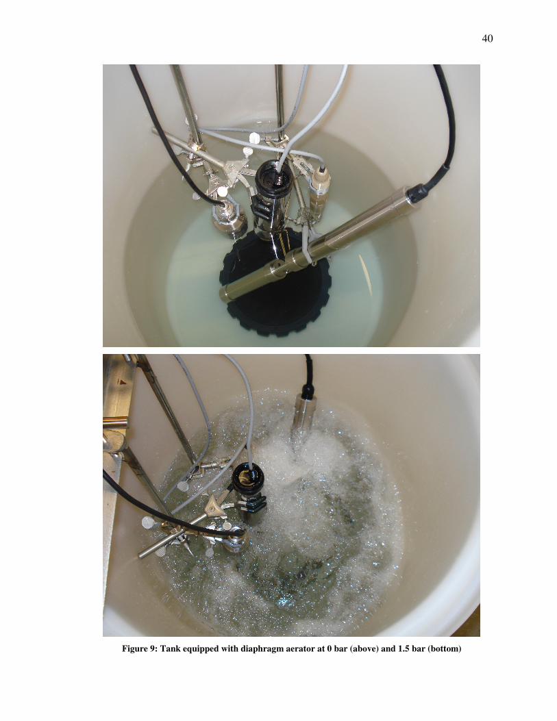
40
Figure 9: Tank equipped with diaphragm aerator at 0 bar (above) and 1.5 bar (bottom)
41
4.3.2 Turbidity
4.3.2.1 Experimental Setup
The effects of turbidity have only been tested on the Spectro::lyser™, because the
other spectrometer and nitrate sensors were not available when this part of the
experimentation was conducted. The Solitax was obviously not tested for effects of
turbidity as it is a turbidity sensor.
The Spectro::lysertm is coming with a recipient that fits around the measuring cell
(see Figure 10). It allows using less solution than when the whole probe is to be immersed
in a tank.
Figure 10: Offline measuring cell for Spectro::lyser™
42
4.3.2.2 Standard
Two different turbidity standards were used: Formazin and AMCO Clear®. The
first issue that has been checked is the stability of the suspension over time. Due to the way
the cell used to make the lab measurements with the Spectro::lyser™ is configured (Figure
10), it is impossible to maintain agitation in the cell. Hence, the importance of evaluating
the stability of the suspension. Two different measurements have been made, first 30
minutes of continuous measurements without touching the sensor or the sampling cell and
another series of 30 minutes while shaking the measuring cell by performing quarter
rotations every minute. Then, the effects of turbidity on the nitrate measurements were
made with the one with better stability.
4.3.2.2.1 Formazin
Formazin is the recognized standard for turbidity. It has even given its name to one
of the units used to quantify turbidity; Formazin Nephelometric Units (FNU). Formazin is
sold in high concentration solutions, and for this experimentation a solution of 4000 FNU
was available. Dilutions were made to get the desired turbidity, i.e. 50 and 10 FNU.
Formazin has the following advantages:
• It is available from most chemical and scientific suppliers
• The least-expensive commercially available standard
and disadvantages:
• It has a Material Safety Data Sheet (MSDS) health-hazard rating of 2:
Rating 2: Intense or continued exposure could cause temporary incapacitation or
possible residual injury unless prompt medical attention is given
(MSDS HyperGlossary, 2009).
• Turbidity can vary by ±2% from batch-to-batch
• The size, shape and aggregation of formazin particles changes with temperature,
time and concentration (see Figure 11).
• It settles during storage and it must be mixed immediately prior to use.
• Diluted formazin standards have a storage life as short as one day (see Table 4).
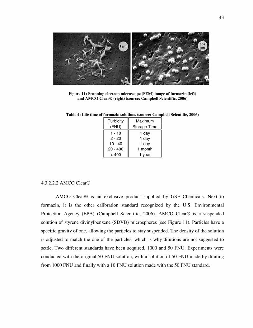
43
Figure 11: Scanning electron microscope (SEM) image of formazin (left)
and AMCO Clear® (right) (source: Campbell Scientific, 2006)
Table 4: Life time of formazin solutions (source: Campbell Scientific, 2006)
Turbidity Maximum
(FNU) Storage Time
1 - 10 1 day
2 - 20 1 day
10 - 40 1 day
20 - 400 1 month
> 400 1 year
4.3.2.2.2 AMCO Clear®
AMCO Clear® is an exclusive product supplied by GSF Chemicals. Next to
formazin, it is the other calibration standard recognized by the U.S. Environmental
Protection Agency (EPA) (Campbell Scientific, 2006). AMCO Clear® is a suspended
solution of styrene divinylbenzene (SDVB) microspheres (see Figure 11). Particles have a
specific gravity of one, allowing the particles to stay suspended. The density of the solution
is adjusted to match the one of the particles, which is why dilutions are not suggested to
settle. Two different standards have been acquired, 1000 and 50 FNU. Experiments were
conducted with the original 50 FNU solution, with a solution of 50 FNU made by diluting
from 1000 FNU and finally with a 10 FNU solution made with the 50 FNU standard.
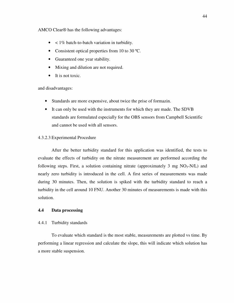
44
AMCO Clear® has the following advantages:
• < 1% batch-to-batch variation in turbidity.
• Consistent optical properties from 10 to 30 ºC.
• Guaranteed one year stability.
• Mixing and dilution are not required.
• It is not toxic.
and disadvantages:
• Standards are more expensive, about twice the prise of formazin.
• It can only be used with the instruments for which they are made. The SDVB
standards are formulated especially for the OBS sensors from Campbell Scientific
and cannot be used with all sensors.
4.3.2.3 Experimental Procedure
After the better turbidity standard for this application was identified, the tests to
evaluate the effects of turbidity on the nitrate measurement are performed according the
following steps. First, a solution containing nitrate (approximately 3 mg NO3-N/L) and
nearly zero turbidity is introduced in the cell. A first series of measurements was made
during 30 minutes. Then, the solution is spiked with the turbidity standard to reach a
turbidity in the cell around 10 FNU. Another 30 minutes of measurements is made with this
solution.
4.4 Data processing
4.4.1 Turbidity standards
To evaluate which standard is the most stable, measurements are plotted vs time. By
performing a linear regression and calculate the slope, this will indicate which solution has
a more stable suspension.
45
4.4.2 Air bubbles and turbidity effects
Three indicators will be used to characterise the effects of air bubbles and turbidity
on the measurements. The first one is the bias generated by the interference. The bias will
be calculated by the difference between the mean of all measurements carried out without
interference in the solution and the mean of the measurements for a particular level of
interference. This will give an idea of the bias generated by the interference. Secondly, the
same thing will be done by calculating the standard deviation. It will give an indication of
the noise level created by the presence of air bubbles or turbidity. Finally, when the
Spectro::lysertm was not able transmit a measurement because it was out of bounds, it gives
NaN (not a number) as result. The number of NaN values obtained will be used as a third
indicator.
4.5 Reference measurements
4.5.1 Nitrate
The nitrate reference measurement was made with the Hach TNT test kit. It is
following a colorimetric method. Test kits are available in two different measuring ranges:
0,23–13,5 (Hach # TNT835) and 5-35 mg/L NO3-N (Hach # TNT836). Measurements were
made with the Hach DR5000 colorimeter.
4.5.2 Turbidity
Turbidity reference measurements were made with a Hach model 2100N
turbidimeter.
CHAPTER V
RESULTS AND DISCUSSION
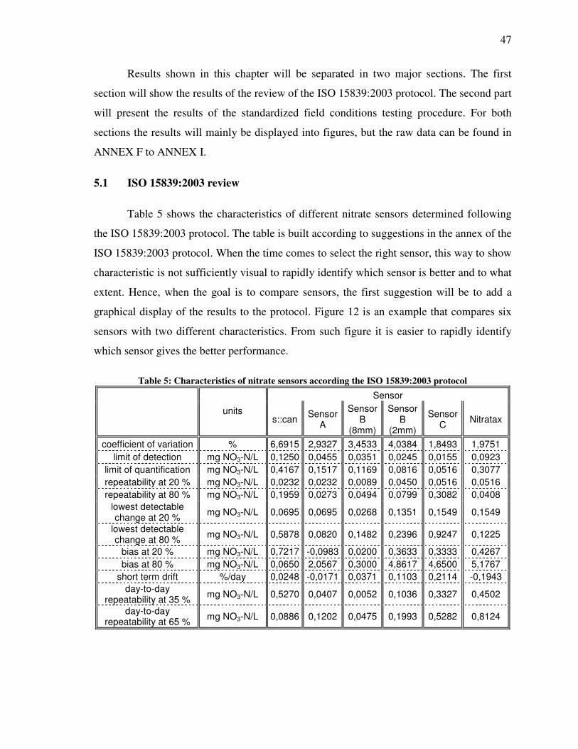
47
Results shown in this chapter will be separated in two major sections. The first
section will show the results of the review of the ISO 15839:2003 protocol. The second part
will present the results of the standardized field conditions testing procedure. For both
sections the results will mainly be displayed into figures, but the raw data can be found in
ANNEX F to ANNEX I.
5.1 ISO 15839:2003 review
Table 5 shows the characteristics of different nitrate sensors determined following
the ISO 15839:2003 protocol. The table is built according to suggestions in the annex of the
ISO 15839:2003 protocol. When the time comes to select the right sensor, this way to show
characteristic is not sufficiently visual to rapidly identify which sensor is better and to what
extent. Hence, when the goal is to compare sensors, the first suggestion will be to add a
graphical display of the results to the protocol. Figure 12 is an example that compares six
sensors with two different characteristics. From such figure it is easier to rapidly identify
which sensor gives the better performance.
Table 5: Characteristics of nitrate sensors according the ISO 15839:2003 protocol
Sensor
units s::can
Sensor A
Sensor B
(8mm)
Sensor B
(2mm)
Sensor C
Nitratax
coefficient of variation % 6,6915 2,9327 3,4533 4,0384 1,8493 1,9751
limit of detection mg NO3-N/L 0,1250 0,0455 0,0351 0,0245 0,0155 0,0923
limit of quantification mg NO3-N/L 0,4167 0,1517 0,1169 0,0816 0,0516 0,3077
repeatability at 20 % mg NO3-N/L 0,0232 0,0232 0,0089 0,0450 0,0516 0,0516
repeatability at 80 % mg NO3-N/L 0,1959 0,0273 0,0494 0,0799 0,3082 0,0408
lowest detectable change at 20 %
mg NO3-N/L 0,0695 0,0695 0,0268 0,1351 0,1549 0,1549
lowest detectable change at 80 %
mg NO3-N/L 0,5878 0,0820 0,1482 0,2396 0,9247 0,1225
bias at 20 % mg NO3-N/L 0,7217 -0,0983 0,0200 0,3633 0,3333 0,4267
bias at 80 % mg NO3-N/L 0,0650 2,0567 0,3000 4,8617 4,6500 5,1767
short term drift %/day 0,0248 -0,0171 0,0371 0,1103 0,2114 -0,1943
day-to-day repeatability at 35 %
mg NO3-N/L 0,5270 0,0407 0,0052 0,1036 0,3327 0,4502
day-to-day repeatability at 65 %
mg NO3-N/L 0,0886 0,1202 0,0475 0,1993 0,5282 0,8124
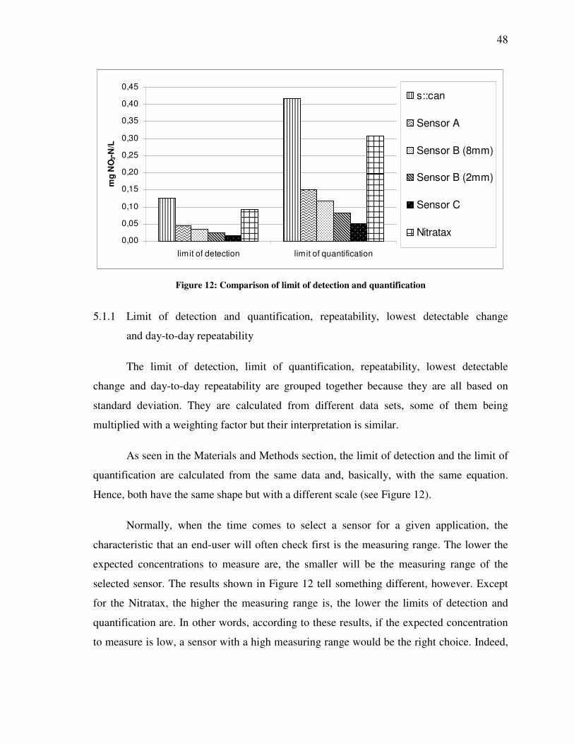
48
0,00
0,05
0,10
0,15
0,20
0,25
0,30
0,35
0,40
0,45
limit of detection limit of quantification
mg
NO
3-N
/L
s::can
Sensor A
Sensor B (8mm)
Sensor B (2mm)
Sensor C
Nitratax
Figure 12: Comparison of limit of detection and quantification
5.1.1 Limit of detection and quantification, repeatability, lowest detectable change
and day-to-day repeatability
The limit of detection, limit of quantification, repeatability, lowest detectable
change and day-to-day repeatability are grouped together because they are all based on
standard deviation. They are calculated from different data sets, some of them being
multiplied with a weighting factor but their interpretation is similar.
As seen in the Materials and Methods section, the limit of detection and the limit of
quantification are calculated from the same data and, basically, with the same equation.
Hence, both have the same shape but with a different scale (see Figure 12).
Normally, when the time comes to select a sensor for a given application, the
characteristic that an end-user will often check first is the measuring range. The lower the
expected concentrations to measure are, the smaller will be the measuring range of the
selected sensor. The results shown in Figure 12 tell something different, however. Except
for the Nitratax, the higher the measuring range is, the lower the limits of detection and
quantification are. In other words, according to these results, if the expected concentration
to measure is low, a sensor with a high measuring range would be the right choice. Indeed,
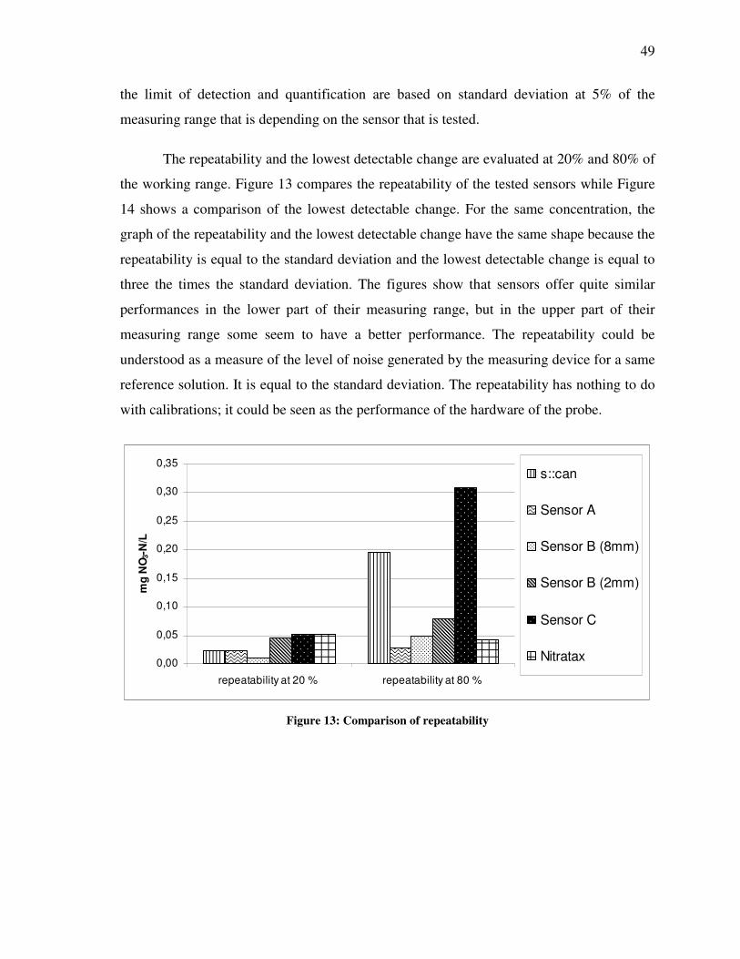
49
the limit of detection and quantification are based on standard deviation at 5% of the
measuring range that is depending on the sensor that is tested.
The repeatability and the lowest detectable change are evaluated at 20% and 80% of
the working range. Figure 13 compares the repeatability of the tested sensors while Figure
14 shows a comparison of the lowest detectable change. For the same concentration, the
graph of the repeatability and the lowest detectable change have the same shape because the
repeatability is equal to the standard deviation and the lowest detectable change is equal to
three the times the standard deviation. The figures show that sensors offer quite similar
performances in the lower part of their measuring range, but in the upper part of their
measuring range some seem to have a better performance. The repeatability could be
understood as a measure of the level of noise generated by the measuring device for a same
reference solution. It is equal to the standard deviation. The repeatability has nothing to do
with calibrations; it could be seen as the performance of the hardware of the probe.
0,00
0,05
0,10
0,15
0,20
0,25
0,30
0,35
repeatability at 20 % repeatability at 80 %
mg
NO
3-N
/L
s::can
Sensor A
Sensor B (8mm)
Sensor B (2mm)
Sensor C
Nitratax
Figure 13: Comparison of repeatability
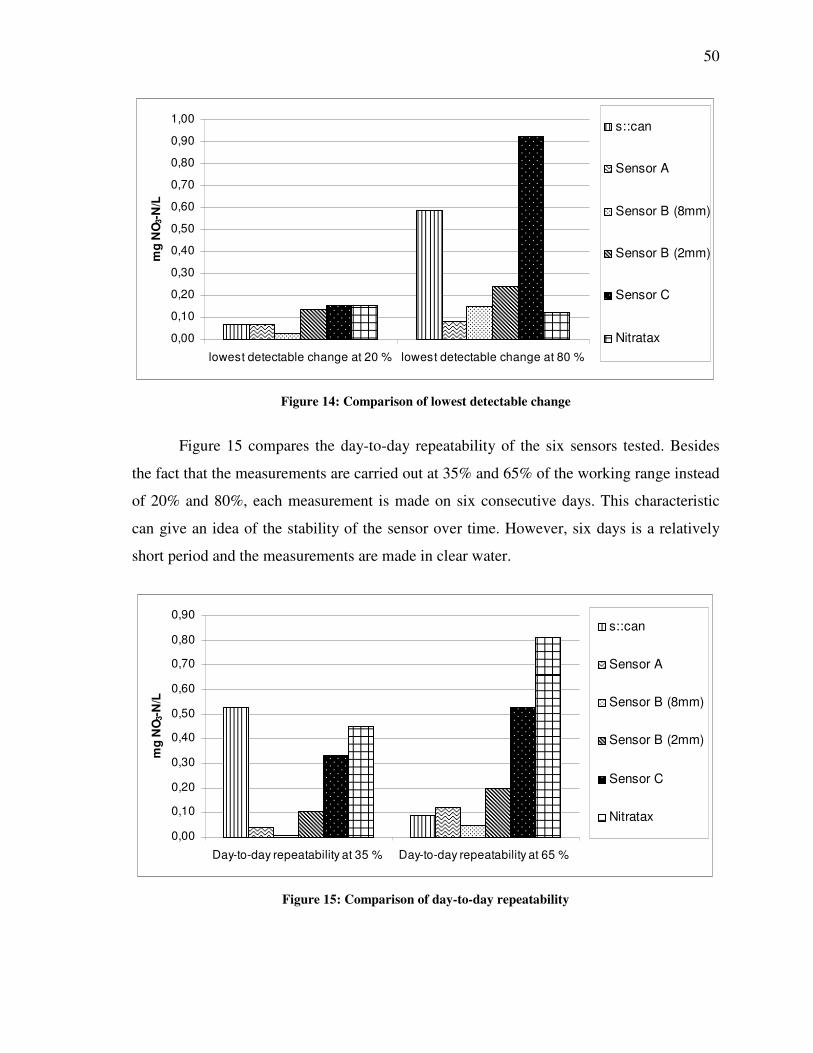
50
0,00
0,10
0,20
0,30
0,40
0,50
0,60
0,70
0,80
0,90
1,00
lowest detectable change at 20 % lowest detectable change at 80 %
mg
NO
3-N
/L
s::can
Sensor A
Sensor B (8mm)
Sensor B (2mm)
Sensor C
Nitratax
Figure 14: Comparison of lowest detectable change
Figure 15 compares the day-to-day repeatability of the six sensors tested. Besides
the fact that the measurements are carried out at 35% and 65% of the working range instead
of 20% and 80%, each measurement is made on six consecutive days. This characteristic
can give an idea of the stability of the sensor over time. However, six days is a relatively
short period and the measurements are made in clear water.
0,00
0,10
0,20
0,30
0,40
0,50
0,60
0,70
0,80
0,90
Day-to-day repeatability at 35 % Day-to-day repeatability at 65 %
mg
NO
3-N
/L
s::can
Sensor A
Sensor B (8mm)
Sensor B (2mm)
Sensor C
Nitratax
Figure 15: Comparison of day-to-day repeatability
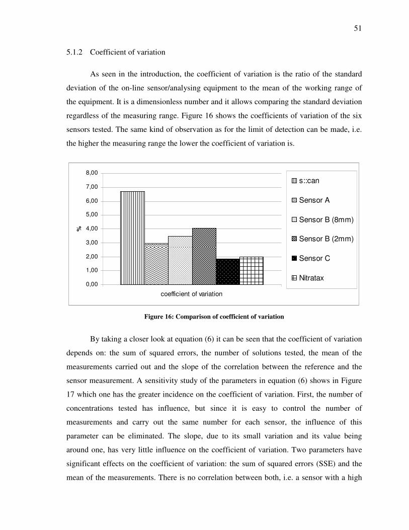
51
5.1.2 Coefficient of variation
As seen in the introduction, the coefficient of variation is the ratio of the standard
deviation of the on-line sensor/analysing equipment to the mean of the working range of
the equipment. It is a dimensionless number and it allows comparing the standard deviation
regardless of the measuring range. Figure 16 shows the coefficients of variation of the six
sensors tested. The same kind of observation as for the limit of detection can be made, i.e.
the higher the measuring range the lower the coefficient of variation is.
0,00
1,00
2,00
3,00
4,00
5,00
6,00
7,00
8,00
coefficient of variation
%
s::can
Sensor A
Sensor B (8mm)
Sensor B (2mm)
Sensor C
Nitratax
Figure 16: Comparison of coefficient of variation
By taking a closer look at equation (6) it can be seen that the coefficient of variation
depends on: the sum of squared errors, the number of solutions tested, the mean of the
measurements carried out and the slope of the correlation between the reference and the
sensor measurement. A sensitivity study of the parameters in equation (6) shows in Figure
17 which one has the greater incidence on the coefficient of variation. First, the number of
concentrations tested has influence, but since it is easy to control the number of
measurements and carry out the same number for each sensor, the influence of this
parameter can be eliminated. The slope, due to its small variation and its value being
around one, has very little influence on the coefficient of variation. Two parameters have
significant effects on the coefficient of variation: the sum of squared errors (SSE) and the
mean of the measurements. There is no correlation between both, i.e. a sensor with a high
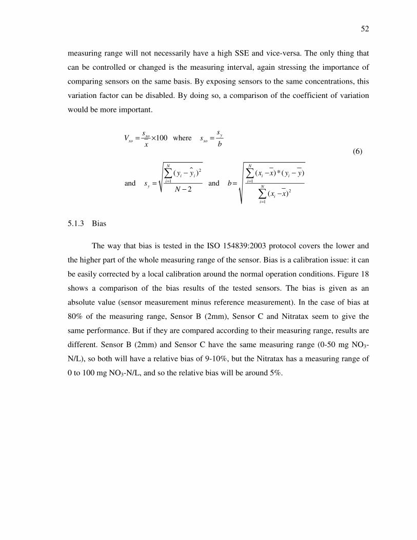
52
measuring range will not necessarily have a high SSE and vice-versa. The only thing that
can be controlled or changed is the measuring interval, again stressing the importance of
comparing sensors on the same basis. By exposing sensors to the same concentrations, this
variation factor can be disabled. By doing so, a comparison of the coefficient of variation
would be more important.
� 2
1 1
2
1
100 where
( ) ( )*( )and and
2 ( )
yxoxo xo
N N
i i ii
i iy N
i
i
ssV s
bx
y y x x y y
s bN
x x
= =
=
= × =
− − −
= =−
−
∑ ∑
∑
(6)
5.1.3 Bias
The way that bias is tested in the ISO 154839:2003 protocol covers the lower and
the higher part of the whole measuring range of the sensor. Bias is a calibration issue: it can
be easily corrected by a local calibration around the normal operation conditions. Figure 18
shows a comparison of the bias results of the tested sensors. The bias is given as an
absolute value (sensor measurement minus reference measurement). In the case of bias at
80% of the measuring range, Sensor B (2mm), Sensor C and Nitratax seem to give the
same performance. But if they are compared according to their measuring range, results are
different. Sensor B (2mm) and Sensor C have the same measuring range (0-50 mg NO3-
N/L), so both will have a relative bias of 9-10%, but the Nitratax has a measuring range of
0 to 100 mg NO3-N/L, and so the relative bias will be around 5%.
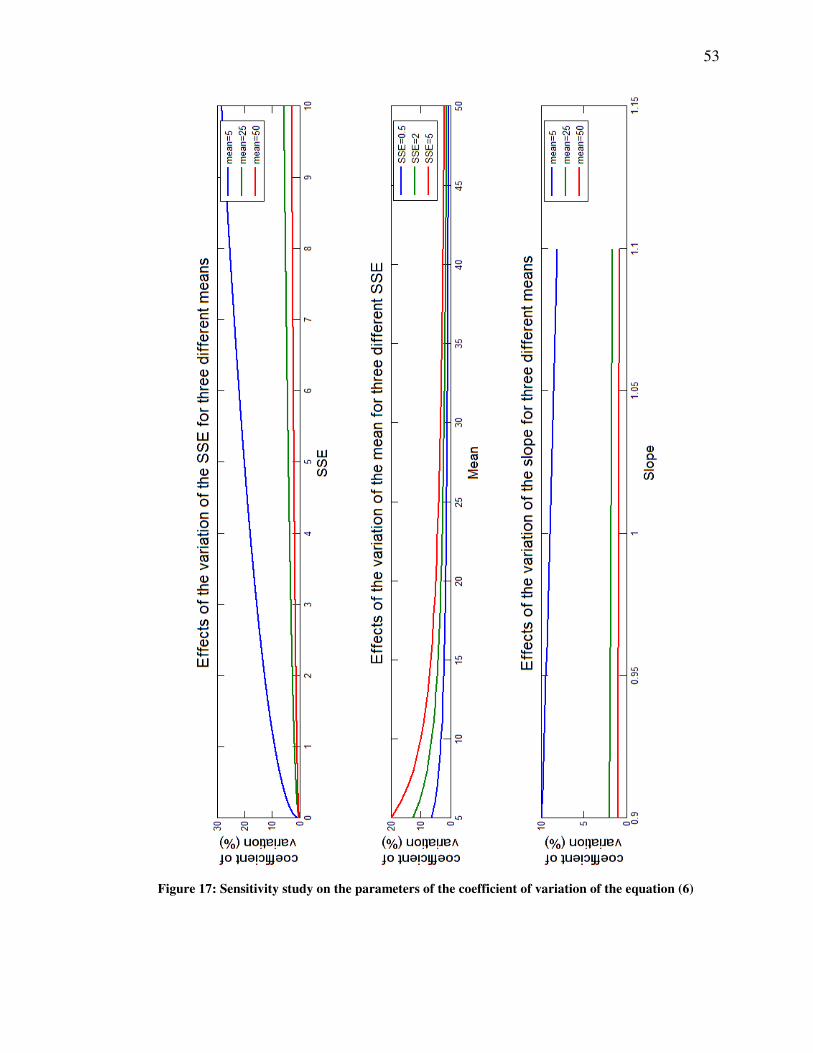
53
Figure 17: Sensitivity study on the parameters of the coefficient of variation of the equation (6)
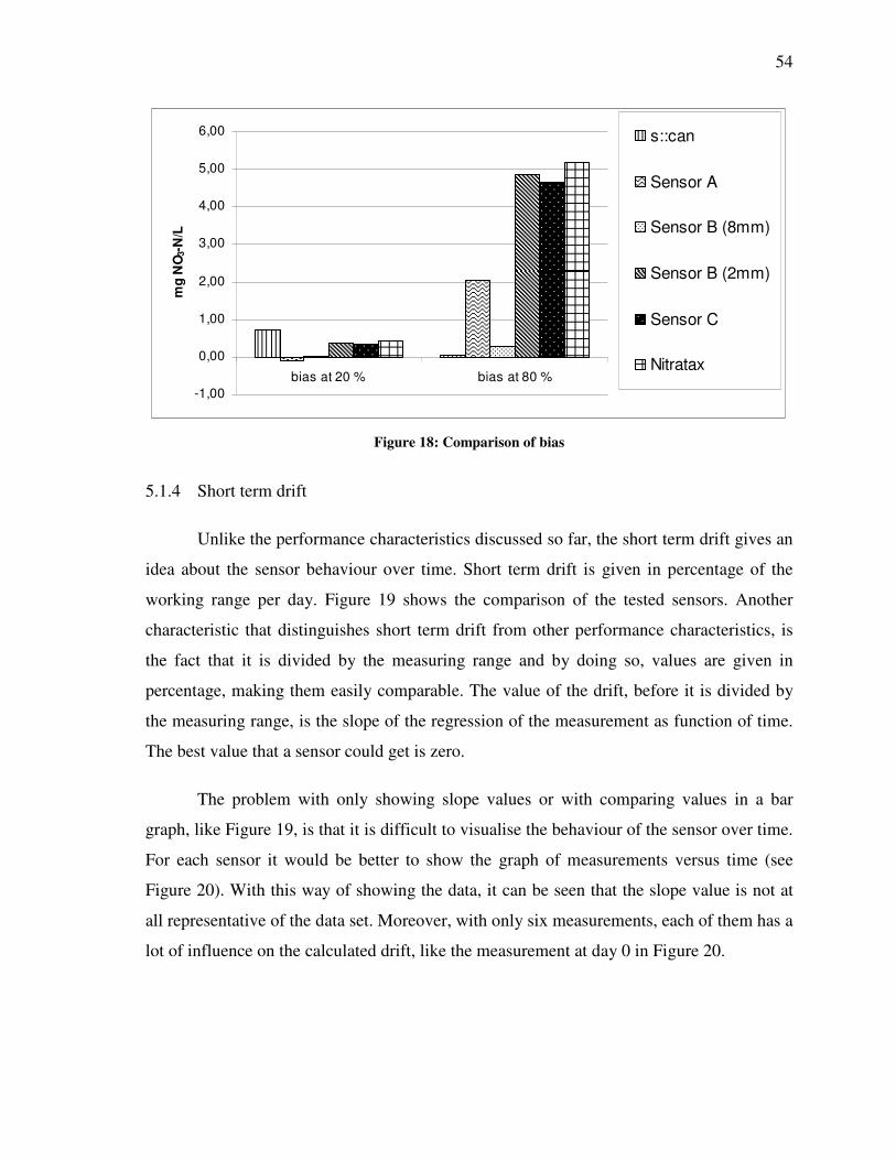
54
-1,00
0,00
1,00
2,00
3,00
4,00
5,00
6,00
bias at 20 % bias at 80 %
mg
NO
3-N
/L
s::can
Sensor A
Sensor B (8mm)
Sensor B (2mm)
Sensor C
Nitratax
Figure 18: Comparison of bias
5.1.4 Short term drift
Unlike the performance characteristics discussed so far, the short term drift gives an
idea about the sensor behaviour over time. Short term drift is given in percentage of the
working range per day. Figure 19 shows the comparison of the tested sensors. Another
characteristic that distinguishes short term drift from other performance characteristics, is
the fact that it is divided by the measuring range and by doing so, values are given in
percentage, making them easily comparable. The value of the drift, before it is divided by
the measuring range, is the slope of the regression of the measurement as function of time.
The best value that a sensor could get is zero.
The problem with only showing slope values or with comparing values in a bar
graph, like Figure 19, is that it is difficult to visualise the behaviour of the sensor over time.
For each sensor it would be better to show the graph of measurements versus time (see
Figure 20). With this way of showing the data, it can be seen that the slope value is not at
all representative of the data set. Moreover, with only six measurements, each of them has a
lot of influence on the calculated drift, like the measurement at day 0 in Figure 20.
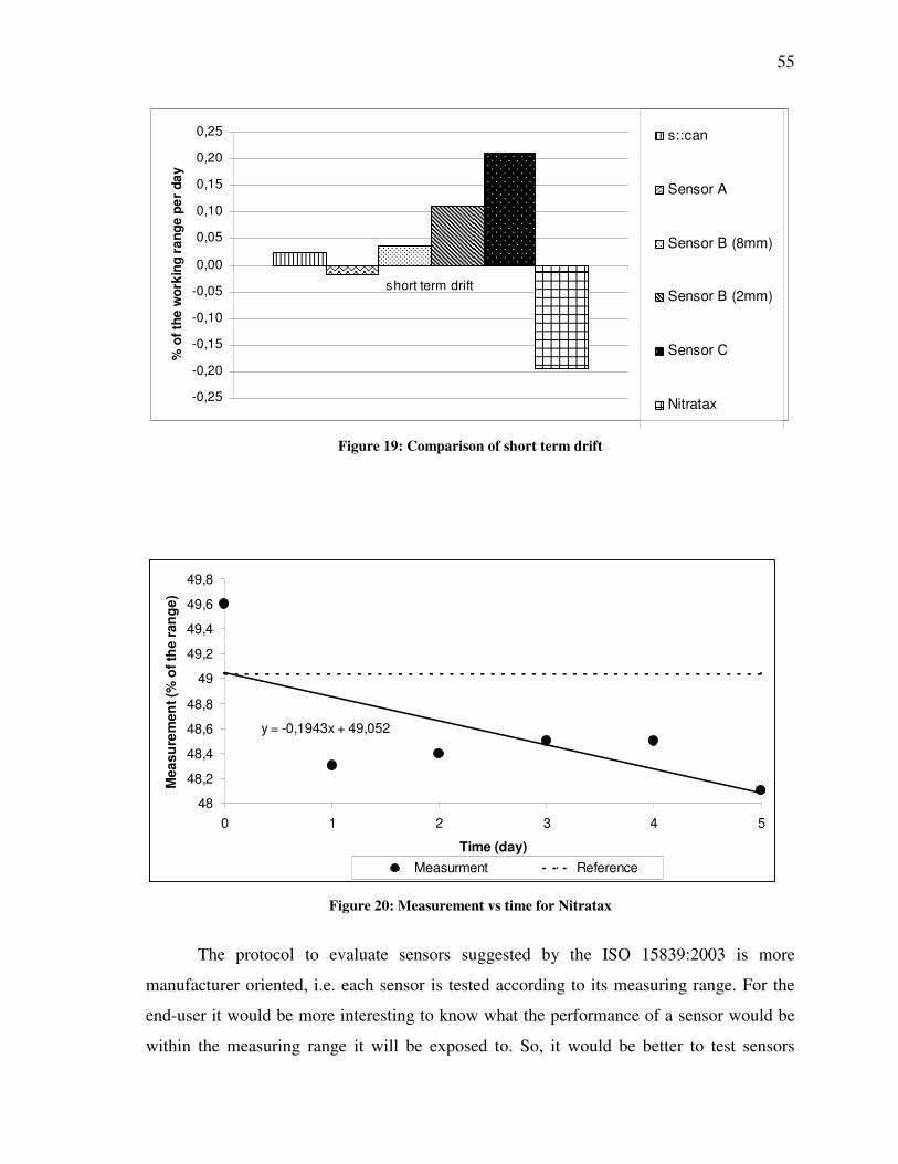
55
-0,25
-0,20
-0,15
-0,10
-0,05
0,00
0,05
0,10
0,15
0,20
0,25
short term drift
% o
f th
e w
ork
ing
ra
ng
e p
er
da
y
s::can
Sensor A
Sensor B (8mm)
Sensor B (2mm)
Sensor C
Nitratax
Figure 19: Comparison of short term drift
y = -0,1943x + 49,052
48
48,2
48,4
48,6
48,8
49
49,2
49,4
49,6
49,8
0 1 2 3 4 5
Time (day)
Mea
su
rem
en
t (%
of
the r
an
ge
)
Measurment Reference
Figure 20: Measurement vs time for Nitratax
The protocol to evaluate sensors suggested by the ISO 15839:2003 is more
manufacturer oriented, i.e. each sensor is tested according to its measuring range. For the
end-user it would be more interesting to know what the performance of a sensor would be
within the measuring range it will be exposed to. So, it would be better to test sensors
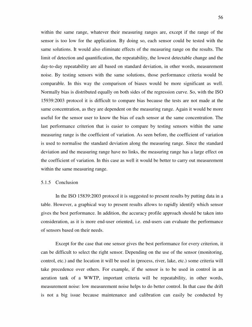
56
within the same range, whatever their measuring ranges are, except if the range of the
sensor is too low for the application. By doing so, each sensor could be tested with the
same solutions. It would also eliminate effects of the measuring range on the results. The
limit of detection and quantification, the repeatability, the lowest detectable change and the
day-to-day repeatability are all based on standard deviation, in other words, measurement
noise. By testing sensors with the same solutions, those performance criteria would be
comparable. In this way the comparison of biases would be more significant as well.
Normally bias is distributed equally on both sides of the regression curve. So, with the ISO
15939:2003 protocol it is difficult to compare bias because the tests are not made at the
same concentration, as they are dependent on the measuring range. Again it would be more
useful for the sensor user to know the bias of each sensor at the same concentration. The
last performance criterion that is easier to compare by testing sensors within the same
measuring range is the coefficient of variation. As seen before, the coefficient of variation
is used to normalise the standard deviation along the measuring range. Since the standard
deviation and the measuring range have no links, the measuring range has a large effect on
the coefficient of variation. In this case as well it would be better to carry out measurement
within the same measuring range.
5.1.5 Conclusion
In the ISO 15839:2003 protocol it is suggested to present results by putting data in a
table. However, a graphical way to present results allows to rapidly identify which sensor
gives the best performance. In addition, the accuracy profile approach should be taken into
consideration, as it is more end-user oriented, i.e. end-users can evaluate the performance
of sensors based on their needs.
Except for the case that one sensor gives the best performance for every criterion, it
can be difficult to select the right sensor. Depending on the use of the sensor (monitoring,
control, etc.) and the location it will be used in (process, river, lake, etc.) some criteria will
take precedence over others. For example, if the sensor is to be used in control in an
aeration tank of a WWTP, important criteria will be repeatability, in other words,
measurement noise: low measurement noise helps to do better control. In that case the drift
is not a big issue because maintenance and calibration can easily be conducted by
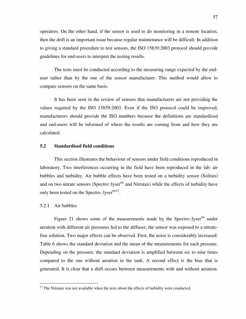
57
operators. On the other hand, if the sensor is used to do monitoring in a remote location,
then the drift is an important issue because regular maintenance will be difficult. In addition
to giving a standard procedure to test sensors, the ISO 15839:2003 protocol should provide
guidelines for end-users to interpret the testing results.
The tests must be conducted according to the measuring range expected by the end-
user rather than by the one of the sensor manufacturer. This method would allow to
compare sensors on the same basis.
It has been seen in the review of sensors that manufacturers are not providing the
values required by the ISO 15839:2003. Even if the ISO protocol could be improved,
manufacturers should provide the ISO numbers because the definitions are standardized
and end-users will be informed of where the results are coming from and how they are
calculated.
5.2 Standardised field conditions
This section illustrates the behaviour of sensors under field conditions reproduced in
laboratory. Two interferences occurring in the field have been reproduced in the lab: air
bubbles and turbidity. Air bubble effects have been tested on a turbidity sensor (Solitax)
and on two nitrate sensors (Spectro::lysertm and Nitratax) while the effects of turbidity have
only been tested on the Spectro::lysertm12.
5.2.1 Air bubbles
Figure 21 shows some of the measurements made by the Spectro::lysertm under
aeration with different air pressures fed to the diffuser; the sensor was exposed to a nitrate-
free solution. Two major effects can be observed. First, the noise is considerably increased:
Table 6 shows the standard deviation and the mean of the measurements for each pressure.
Depending on the pressure, the standard deviation is amplified between six to nine times
compared to the one without aeration in the tank. A second effect is the bias that is
generated. It is clear that a shift occurs between measurements with and without aeration.
12 The Nitratax was not available when the tests about the effects of turbidity were conducted.
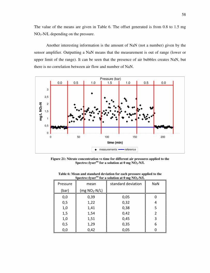
58
The value of the means are given in Table 6. The offset generated is from 0.8 to 1.5 mg
NO3-N/L depending on the pressure.
Another interesting information is the amount of NaN (not a number) given by the
sensor amplifier. Outputting a NaN means that the measurement is out of range (lower or
upper limit of the range). It can be seen that the presence of air bubbles creates NaN, but
there is no correlation between air flow and number of NaN.
0
0,5
1
1,5
2
2,5
3
0 50 100 150 200
time (min)
mg
/L N
O3-N
measurements reference
0.0 0.5 1.0 1.5 1.0 0.5 0.0Pressure (bar)
Figure 21: Nitrate concentration vs time for different air pressures applied to the
Spectro::lysertm for a solution at 0 mg NO3-N/L
Table 6: Mean and standard deviation for each pressure applied to the Spectro::lysertm for a solution at 0 mg NO3-N/L
Pressure mean standard deviation NaN
(bar) (mg NO3-N/L)
0,0 0,39 0,05 0
0,5 1,22 0,32 4
1,0 1,41 0,38 5
1,5 1,54 0,42 2
1,0 1,51 0,45 3
0,5 1,29 0,35 6
0,0 0,42 0,05 0
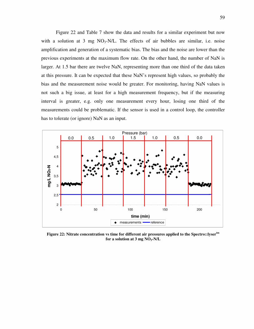
59
Figure 22 and Table 7 show the data and results for a similar experiment but now
with a solution at 3 mg NO3-N/L. The effects of air bubbles are similar, i.e. noise
amplification and generation of a systematic bias. The bias and the noise are lower than the
previous experiments at the maximum flow rate. On the other hand, the number of NaN is
larger. At 1.5 bar there are twelve NaN, representing more than one third of the data taken
at this pressure. It can be expected that these NaN’s represent high values, so probably the
bias and the measurement noise would be greater. For monitoring, having NaN values is
not such a big issue, at least for a high measurement frequency, but if the measuring
interval is greater, e.g. only one measurement every hour, losing one third of the
measurements could be problematic. If the sensor is used in a control loop, the controller
has to tolerate (or ignore) NaN as an input.
2
2,5
3
3,5
4
4,5
5
0 50 100 150 200
time (min)
mg
/L N
O3-N
measurements reference
0.0 0.5 1.0 1.5 1.0 0.5 0.0Pressure (bar)
Figure 22: Nitrate concentration vs time for different air pressures applied to the Spectro::lysertm
for a solution at 3 mg NO3-N/L
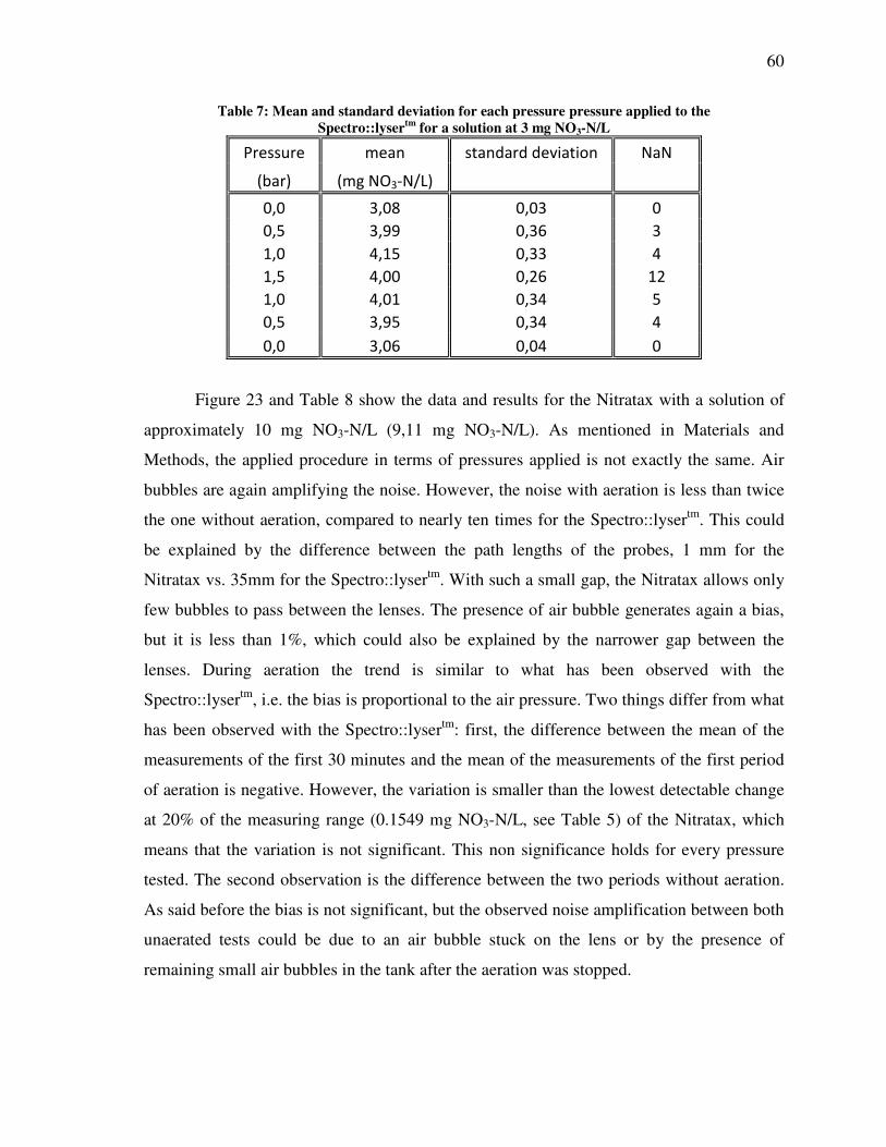
60
Table 7: Mean and standard deviation for each pressure pressure applied to the Spectro::lysertm for a solution at 3 mg NO3-N/L
Pressure mean standard deviation NaN
(bar) (mg NO3-N/L)
0,0 3,08 0,03 0
0,5 3,99 0,36 3
1,0 4,15 0,33 4
1,5 4,00 0,26 12
1,0 4,01 0,34 5
0,5 3,95 0,34 4
0,0 3,06 0,04 0
Figure 23 and Table 8 show the data and results for the Nitratax with a solution of
approximately 10 mg NO3-N/L (9,11 mg NO3-N/L). As mentioned in Materials and
Methods, the applied procedure in terms of pressures applied is not exactly the same. Air
bubbles are again amplifying the noise. However, the noise with aeration is less than twice
the one without aeration, compared to nearly ten times for the Spectro::lysertm. This could
be explained by the difference between the path lengths of the probes, 1 mm for the
Nitratax vs. 35mm for the Spectro::lysertm. With such a small gap, the Nitratax allows only
few bubbles to pass between the lenses. The presence of air bubble generates again a bias,
but it is less than 1%, which could also be explained by the narrower gap between the
lenses. During aeration the trend is similar to what has been observed with the
Spectro::lysertm, i.e. the bias is proportional to the air pressure. Two things differ from what
has been observed with the Spectro::lysertm: first, the difference between the mean of the
measurements of the first 30 minutes and the mean of the measurements of the first period
of aeration is negative. However, the variation is smaller than the lowest detectable change
at 20% of the measuring range (0.1549 mg NO3-N/L, see Table 5) of the Nitratax, which
means that the variation is not significant. This non significance holds for every pressure
tested. The second observation is the difference between the two periods without aeration.
As said before the bias is not significant, but the observed noise amplification between both
unaerated tests could be due to an air bubble stuck on the lens or by the presence of
remaining small air bubbles in the tank after the aeration was stopped.
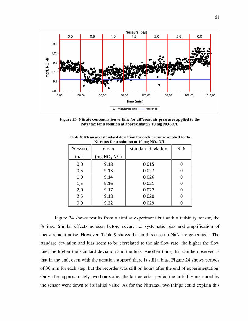
61
9,05
9,1
9,15
9,2
9,25
9,3
0,00 30,00 60,00 90,00 120,00 150,00 180,00 210,00
time (min)
mg
/L N
O3-N
measurements reference
0.0 0.5 1.0 1.5 2.0 2.5 0.0
Pressure (bar)
Figure 23: Nitrate concentration vs time for different air pressures applied to the
Nitratax for a solution at approximately 10 mg NO3-N/L
Table 8: Mean and standard deviation for each pressure applied to the Nitratax for a solution at 10 mg NO3-N/L
Pressure mean standard deviation NaN
(bar) (mg NO3-N/L)
0,0 9,18 0,015 0
0,5 9,13 0,027 0
1,0 9,14 0,026 0
1,5 9,16 0,021 0
2,0 9,17 0,022 0
2,5 9,18 0,020 0
0,0 9,22 0,029 0
Figure 24 shows results from a similar experiment but with a turbidity sensor, the
Solitax. Similar effects as seen before occur, i.e. systematic bias and amplification of
measurement noise. However, Table 9 shows that in this case no NaN are generated. The
standard deviation and bias seem to be correlated to the air flow rate; the higher the flow
rate, the higher the standard deviation and the bias. Another thing that can be observed is
that in the end, even with the aeration stopped there is still a bias. Figure 24 shows periods
of 30 min for each step, but the recorder was still on hours after the end of experimentation.
Only after approximately two hours after the last aeration period the turbidity measured by
the sensor went down to its initial value. As for the Nitratax, two things could explain this
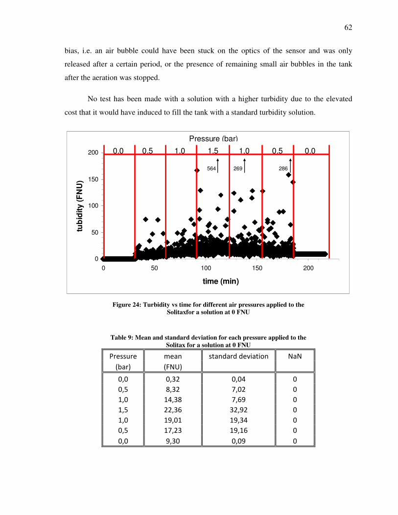
62
bias, i.e. an air bubble could have been stuck on the optics of the sensor and was only
released after a certain period, or the presence of remaining small air bubbles in the tank
after the aeration was stopped.
No test has been made with a solution with a higher turbidity due to the elevated
cost that it would have induced to fill the tank with a standard turbidity solution.
0
50
100
150
200
0 50 100 150 200
time (min)
tub
idit
y (
FN
U)
0.0 0.5 1.0 1.5 1.0 0.5 0.0
Pressure (bar)
564 269 286
Figure 24: Turbidity vs time for different air pressures applied to the
Solitaxfor a solution at 0 FNU
Table 9: Mean and standard deviation for each pressure applied to the Solitax for a solution at 0 FNU
Pressure mean standard deviation NaN
(bar) (FNU)
0,0 0,32 0,04 0
0,5 8,32 7,02 0
1,0 14,38 7,69 0
1,5 22,36 32,92 0
1,0 19,01 19,34 0
0,5 17,23 19,16 0
0,0 9,30 0,09 0
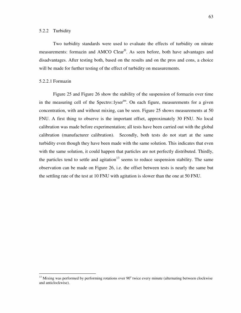
63
5.2.2 Turbidity
Two turbidity standards were used to evaluate the effects of turbidity on nitrate
measurements: formazin and AMCO Clear®. As seen before, both have advantages and
disadvantages. After testing both, based on the results and on the pros and cons, a choice
will be made for further testing of the effect of turbidity on measurements.
5.2.2.1 Formazin
Figure 25 and Figure 26 show the stability of the suspension of formazin over time
in the measuring cell of the Spectro::lysertm. On each figure, measurements for a given
concentration, with and without mixing, can be seen. Figure 25 shows measurements at 50
FNU. A first thing to observe is the important offset, approximately 30 FNU. No local
calibration was made before experimentation; all tests have been carried out with the global
calibration (manufacturer calibration). Secondly, both tests do not start at the same
turbidity even though they have been made with the same solution. This indicates that even
with the same solution, it could happen that particles are not perfectly distributed. Thirdly,
the particles tend to settle and agitation13 seems to reduce suspension stability. The same
observation can be made on Figure 26, i.e. the offset between tests is nearly the same but
the settling rate of the test at 10 FNU with agitation is slower than the one at 50 FNU.
13 Mixing was performed by performing rotations over 90o twice every minute (alternating between clockwise and anticlockwise).
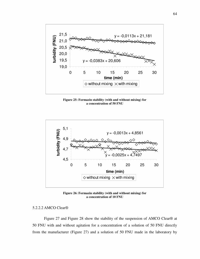
64
y = -0,0113x + 21,181
y = -0,0383x + 20,606
19,0
19,5
20,0
20,5
21,0
21,5
0 5 10 15 20 25 30
time (min)
turb
idit
y (
FN
U)
without mixing with mixing
Figure 25: Formazin stability (with and without mixing) for
a concentration of 50 FNU
y = -0,0013x + 4,8561
y = -0,0025x + 4,74974,5
4,7
4,9
5,1
0 5 10 15 20 25 30
time (min)
turb
idit
y (
FN
U)
without mixing with mixing
Figure 26: Formazin stability (with and without mixing) for
a concentration of 10 FNU
5.2.2.2 AMCO Clear®
Figure 27 and Figure 28 show the stability of the suspension of AMCO Clear® at
50 FNU with and without agitation for a concentration of a solution of 50 FNU directly
from the manufacturer (Figure 27) and a solution of 50 FNU made in the laboratory by
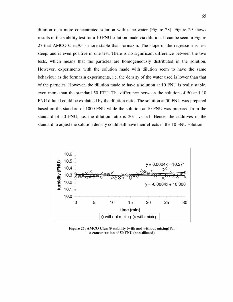
65
dilution of a more concentrated solution with nano-water (Figure 28). Figure 29 shows
results of the stability test for a 10 FNU solution made via dilution. It can be seen in Figure
27 that AMCO Clear® is more stable than formazin. The slope of the regression is less
steep, and is even positive in one test. There is no significant difference between the two
tests, which means that the particles are homogeneously distributed in the solution.
However, experiments with the solution made with dilution seem to have the same
behaviour as the formazin experiments, i.e. the density of the water used is lower than that
of the particles. However, the dilution made to have a solution at 10 FNU is really stable,
even more than the standard 50 FTU. The difference between the solution of 50 and 10
FNU diluted could be explained by the dilution ratio. The solution at 50 FNU was prepared
based on the standard of 1000 FNU while the solution at 10 FNU was prepared from the
standard of 50 FNU, i.e. the dilution ratio is 20:1 vs 5:1. Hence, the additives in the
standard to adjust the solution density could still have their effects in the 10 FNU solution.
y = -0,0004x + 10,308
y = 0,0024x + 10,271
10,0
10,1
10,2
10,3
10,4
10,5
10,6
0 5 10 15 20 25 30
time (min)
turb
idit
y (
FN
U)
without mixing with mixing
Figure 27: AMCO Clear® stability (with and without mixing) for
a concentration of 50 FNU (non-diluted)
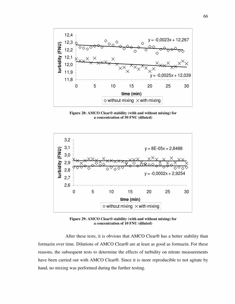
66
y = -0,0023x + 12,267
y = -0,0025x + 12,03911,8
11,9
12,0
12,1
12,2
12,3
12,4
0 5 10 15 20 25 30
time (min)
turb
idit
y (
FN
U)
without mixing with mixing
Figure 28: AMCO Clear® stability (with and without mixing) for
a concentration of 50 FNU (diluted)
y = 8E-05x + 2,8488
y = -0,0002x + 2,9254
2,6
2,7
2,8
2,9
3,0
3,1
3,2
0 5 10 15 20 25 30
time (min)
turb
idit
y (
FN
U)
without mixing with mixing
Figure 29: AMCO Clear® stability (with and without mixing) for
a concentration of 10 FNU (diluted)
After these tests, it is obvious that AMCO Clear® has a better stability than
formazin over time. Dilutions of AMCO Clear® are at least as good as formazin. For these
reasons, the subsequent tests to determine the effects of turbidity on nitrate measurements
have been carried out with AMCO Clear®. Since it is more reproducible to not agitate by
hand, no mixing was performed during the further testing.
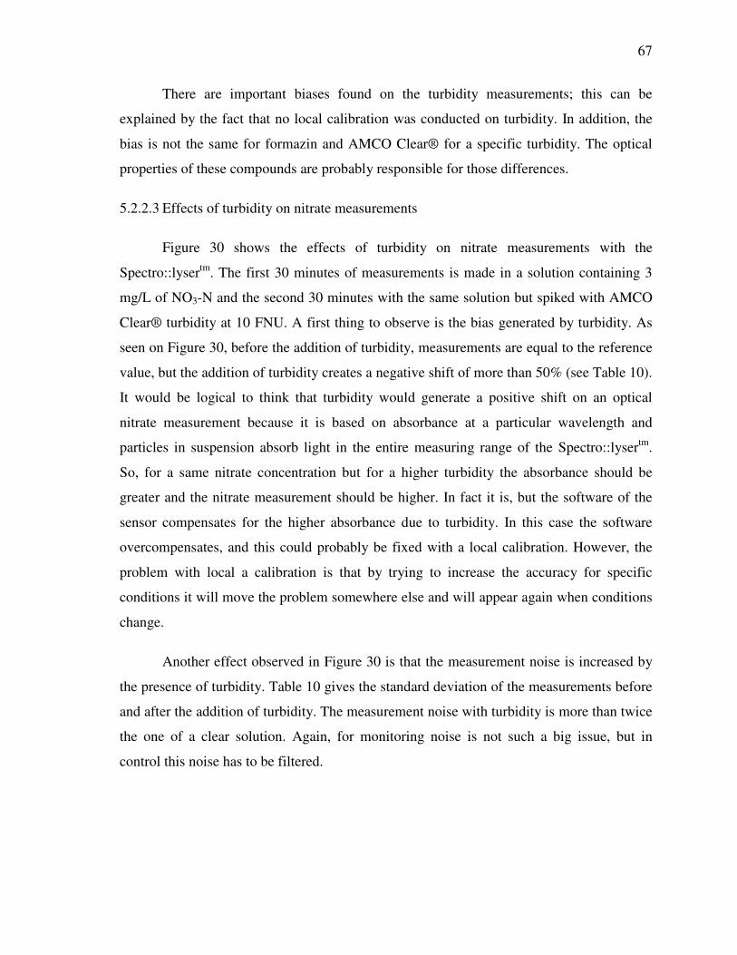
67
There are important biases found on the turbidity measurements; this can be
explained by the fact that no local calibration was conducted on turbidity. In addition, the
bias is not the same for formazin and AMCO Clear® for a specific turbidity. The optical
properties of these compounds are probably responsible for those differences.
5.2.2.3 Effects of turbidity on nitrate measurements
Figure 30 shows the effects of turbidity on nitrate measurements with the
Spectro::lysertm. The first 30 minutes of measurements is made in a solution containing 3
mg/L of NO3-N and the second 30 minutes with the same solution but spiked with AMCO
Clear® turbidity at 10 FNU. A first thing to observe is the bias generated by turbidity. As
seen on Figure 30, before the addition of turbidity, measurements are equal to the reference
value, but the addition of turbidity creates a negative shift of more than 50% (see Table 10).
It would be logical to think that turbidity would generate a positive shift on an optical
nitrate measurement because it is based on absorbance at a particular wavelength and
particles in suspension absorb light in the entire measuring range of the Spectro::lysertm.
So, for a same nitrate concentration but for a higher turbidity the absorbance should be
greater and the nitrate measurement should be higher. In fact it is, but the software of the
sensor compensates for the higher absorbance due to turbidity. In this case the software
overcompensates, and this could probably be fixed with a local calibration. However, the
problem with local a calibration is that by trying to increase the accuracy for specific
conditions it will move the problem somewhere else and will appear again when conditions
change.
Another effect observed in Figure 30 is that the measurement noise is increased by
the presence of turbidity. Table 10 gives the standard deviation of the measurements before
and after the addition of turbidity. The measurement noise with turbidity is more than twice
the one of a clear solution. Again, for monitoring noise is not such a big issue, but in
control this noise has to be filtered.
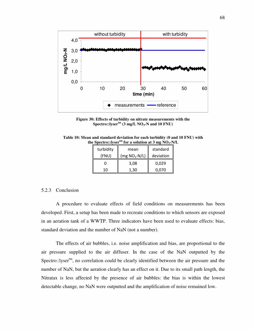
68
0,0
1,0
2,0
3,0
4,0
0 10 20 30 40 50 60
time (min)
mg
/L N
O3-N
measurements reference
without turbidity with turbidity
Figure 30: Effects of turbidity on nitrate measurements with the
Spectro::lysertm (3 mg/L NO3-N and 10 FNU)
Table 10: Mean and standard deviation for each turbidity (0 and 10 FNU) with the Spectro::lysertm for a solution at 3 mg NO3-N/L
turbidity mean standard
(FNU) (mg NO3-N/L) deviation
0 3,08 0,029
10 1,30 0,070
5.2.3 Conclusion
A procedure to evaluate effects of field conditions on measurements has been
developed. First, a setup has been made to recreate conditions to which sensors are exposed
in an aeration tank of a WWTP. Three indicators have been used to evaluate effects: bias,
standard deviation and the number of NaN (not a number).
The effects of air bubbles, i.e. noise amplification and bias, are proportional to the
air pressure supplied to the air diffuser. In the case of the NaN outputted by the
Spectro::lysertm, no correlation could be clearly identified between the air pressure and the
number of NaN, but the aeration clearly has an effect on it. Due to its small path length, the
Nitratax is less affected by the presence of air bubbles: the bias is within the lowest
detectable change, no NaN were outputted and the amplification of noise remained low.
69
The second interference simulated was turbidity. Tests to see which turbidity
standard, formazin or AMCO Clear®, is the most stable shows that AMCO Clear® settles
less than formazin, even when dilutions are made. In addition, AMCO Clear® has the
advantages of being non toxic, having a more uniform particle size and having a longer
shelf life. The same indicators of interference as for the air bubbles have been used. In this
case no NaN occurred. In the case of the Spectro::lyser™, the presence of turbidity
generated a negative bias and the standard deviation was increased.
The two simulated field conditions demonstrate that there is a gap between
laboratory measurements and field measurements. End-users without a lot of knowledge
about sensors, cannot predict, based on the laboratory performance of sensors, how sensors
will behave during field operation. This is why there is a need for a standardized protocol
for testing sensors under field conditions.

CHAPTER VI
CONCLUSION
71
6.1 Study summary
6.1.1 Protocol and sensors review
This study had two main objectives. The first one was to characterise sensors
according to available protocols in order to evaluate the performance of on-line and in-line
sensors in the water quality field and to determine whether the results of those tests are
meaningful and useful to select the right sensor for a specific application.
The principle protocol available for this is the ISO 15839:2003 protocol, Water
quality – On-line sensors/analysing equipment for water - Specifications and performances
tests. First a sensors review was made to see whether manufacturers are providing ISO data
about their sensors. The review has been made for sensors measuring the following
compounds: nitrate, nitrite, ammonia, phosphate, dissolved oxygen and turbidity. The
review showed that companies are providing really little information defined in the ISO
15839:2003 protocol. To figure out why companies are not providing information of the
ISO 15839:2003 protocol, it has been critically reviewed.
The ISO 15839:2003 protocol has two main parts. The first one is for laboratory
testing which gives the performance of sensors in reproducible conditions. Advantages of
this part of the protocol are that the sensors can be compared on the same basis and results
do not depend on the place and the time the tests are made. On the other hand, this part of
the protocol does not help to predict what the sensor behaviour will be under field
conditions. Six nitrate sensors using an optical measuring principle were subject to the
laboratory tests for the review of this part of the protocol.
The results showed that when sensors have different measuring ranges, it would be
better to test the sensors for a given, common measuring range so as to compare the
performance characteristics obtained. Emphasis should be put on a graphical presentation
of the data rather than just providing numbers, e.g. the short term drift (see Figure 19) or
the accuracy profile where many characteristics can be calculated. The ISO 15839:2003
protocol is manufacturer oriented, and it should be more oriented to end-users to help them
select the right sensors for their specific application. Guidelines should be added to the ISO
72
protocol to help end-users understand the performance criteria and to help them to know on
which criteria they should put the emphasis for their application.
The second part of the ISO 15839:2003 protocol is about field testing. This part of
the protocol is to evaluate the performance of sensors under specific field conditions. It has
the disadvantage of being time and site specific, which does not give the opportunity to
compare different sensors if they are not tested at the same time in the same place. The
sensor review showed that there are different measuring principles for each compound and
each of them reacts in different way to interferences. Since one of the goals is compare
sensors, a need for standardized field conditions has occurred.
6.1.2 Standardized field conditions
The second goal of this study was to develop a protocol reproducing conditions to
which sensors are exposed while they are measuring and to evaluate effects of those
perturbations.
Two different potential interferences have been selected: presence of air bubbles
and turbidity. The effects of air bubbles have been tested on a spectrometer and on a
turbidity sensor while the effects of turbidity have only been tested on a spectrometer. Air
bubbles have different effects. They increase the measurement noise and they also generate
an offset. Finally in the case of the spectrometer, when the measurements exceed the upper
limit of the measuring range, the probe is giving NaN (not a number).
The nitrate measurement with the Spectro::lysertm is influenced by the presence of
turbidity in the solution. It increases the noise level and it generates a negative offset. This
offset comes from the fact that the software tries to compensate for the presence of
turbidity.
It also has been concluded that AMCO Clear® is a better product than formazin to
carry out turbidity tests due to its greater stability, more homogeneous particle size and it is
non toxic.
73
The standardised field conditions testing procedure is helpful to compare sensors
and predict which one would give better performance under field operation. It would help
end-users to select sensors according to their application in a far better way than if they
only can be using laboratory performance information.
6.2 Further work
This study has helped to go deeper into sensors characterisation. Regarding sensor
characterisation of performances in the laboratory it would be interesting to test sensors
according to the accuracy profiles (Hubert et al., 2004) to see how it could be integrated
into standard protocols already in place. It would be important to extend the review of
protocols on others measuring principles and on others compounds.
Concerning the standardized field conditions, it would be important to extend the
proposed tests to other interferences (such as pH, ionic strength, temperature, etc.). So far,
only two interferences have been tested for one measuring principle. For instance, an
important issue for sensor operation is fouling, often caused by the formation of biofilms at
the surface of the sensors. By simulating the occurrence of biofilms, effects on
measurements could be tested and the efficiency of auto-cleaning systems as well.
Due to a lack of information provided by the manufacturers, cost could not been
taken into account. It should have been included into the selection procedure, not only
including the investment costs but all the costs presented in Table 2, i.e. maintenance,
installation, consumables, etc. Lifecycle assessment could also be studied and included in
selection criteria for sensors.

REFERENCES
75
APHA (1992). Standard Methods for the Examination of Water and Wastewater, 18th ed. Washington DC. Andersen, K.L. and Wagner, P. (1990). Testing on-line monitors for ammonia, orthophosphate and suspended solids in activated sludge treatment plants. In: Instrumentation, Control and Automation of Water and Wastewater Treatment and
Transport Systems (Advances in Water Pollution Control 10). Ed. Briggs R., Pergamon Press, London, 667–675. Aspegren, H., Nyberg, U. and Andersson, B. (1993). Integration of on-line instruments in the practical operation of the Klagshamn wastewater treatment plant. Med. Fac.
Landbouww. Univ. Gent, 58, 2019–2028. Automation of Wastewater Treatment Facilities (2005). Water Environment Federation/McGraw-Hill, Alexandria, USA. Barnard, J.L. and Crowther, R. (1993). Instrumentation in biological nutrient removal plants. In: Preprints of 6th IAWQ Workshop on ICA of Water and Wastewater
Treatment and Transport Systems. June 17–19, Banff, Canada. Blake-Coleman, B.C., Clarke, D.J., Calder, M.R. and Moody, S.C. (1986). Determination of reactor biomass by acoustic-resonance densitometry. Biotech. Bioeng., 28, 1241 1249. Cammann, K. and Schroeder, A. (1979). Working with Ion-Selective Electrodes. ISBN 0387-09320-6. Springer Verlag, New York, USA. Campbell Scientific (2006). Turbidity Standards: http://www.d-a-instruments.com /turbidity_standards.html (accessed 20 July 2009) Davey, C.L., Davey, H.M., Kell, D.B. and Todd, R.W. (1993). Introduction to the dielectric estimation of cellular biomass in real-time, with special emphasis on measurements at high-volume fractions. Anal. Chim. Acta., 279, 155–161. Dobbs, R.A., Wise, R.H. and Dean, R.B. (1972). The use of ultra-violet absorbance for monitoring the total organic carbon of water and wastewater. Wat. Res., 6, 1173 1180. Endress+Hauser (2006a). Measuring Dissolved Oxygen – OxyMax W COS 31. Endress+Hauser (2006b). OxyMax W COS 61- Dissolved oxygen measurement. EURACHEM (1998). The Fitness for Purpose of Analytical Methods. Edition 1.0, LGC (Teddington) Gippel, C.J. (1995). Potential of turbidity monitoring for mmeasuring the transport of suspended-solids in streams. Hydrol. Proc., 9(1), 83-87.
76
Hach (2005). Hach LDO® Dissolved Oxygen Probe. Lit. No. 2455. Printed in USA. Harremoës, P., Capodaglio, A.G., Hellström, B.G., Henze, M., Jensen, K.N., Lynggaard Jensen, A., Otterpohl, R. and Soeberg, H. (1993). Wastewater treatment plants under transient loading – performance, modelling and control. Wat. Sci. Tech., 27(12), 71–115. Hauduc, H. (2007). L’Application de la Méthode des Profils d’Exactitudes à Différentes
Techniques d’Analyses Environnementales. M.Sc thesis, AgroParisTech/brgm, Paris, France. Hubert, P., Nguyen-Huu, J.-J., Boulanger, B., Chapuzet, E., Chiap, P., Cohen, N., Compagnon, P.-A., Dew’e, W., Feinberg, M., Lallier, M., Laurentie, M., Mercier, N., Muzard, G., Nivet, C. and Valat, L. (2004). Harmonisation of strategies for the validation of quantitative analytical procedures. A SFSTP propsal – part I. J.
Pharm. Biomedi. Anal., 36(2004), 579-586. ISO (2008). Water quality – On-line sensors/analysing equipment for water –
Specifications and performances tests, ISO Standard 15839, Geneva, Switzerland. Jones, A., Young, D., Taylor, J., Kell, D.B. and Rowland, J.J. (1998). Quantification of Microbial productivity via multi-angle light scattering and supervised learning. Biotech. Bioeng., 59, 131–143. Lynggaard-Jensen, A., Eisum, N.H., Rasmussen, I., Svankjær Jocobsen, H. and Stenstrøm, T. (1996). Description and test of a new generation of nutrient sensors. Wat. Sci.
Tech., 33(1), 25–35. MacCraith, B., Grattan, K.T.V., Connolly, D., Briggs, R., Boyle, W.J.O. and Avis, M. (1993). Cross comparison of techniques for the monitoring of total organic carbon (TOC) in water resources and supplies. Wat. Sci. Tech., 28(11–12), 457–463. MSDS HyperGlossary (2009). ILPI: http://www.ilpi.com/MSDS/ref/nfpa.html (accessed 01 August 2009) November, E.J. and Van Impe, J.F. (2001). On-line viable biomass measurement and estimation of the specific growth rate of activated sludge from municipal wastewater treatment. Wat. Sci. Tech., 43(7), 97–102. Olsson, L. and Nielsen, J. (1997). On-line and in situ monitoring of biomass in submerged cultivations. TIBTECH, 15, 517–522. Olsson, G., Nielsen, M.K., Yuan, Z., Lynggaard-Jensen, A. and Steyer, J.P. (2005). Instrumentation, Control and Automation in Wastewater Systems. IWA, London, USA.
77
Oxford Online Dictionary (2005). University Press: http://www.oup.com/oald bin/web_getald7index1a.pl?search_word=Accuracy (accessed 07 July 2009) Patry, G.G. and Takács, I. (1995). Modelling, simulation and control of large-scale wastewater treatment plants: an integrated approach. Med. Fac. Landbouww. Univ.
Gent, 60, 2335–2343. Petersen, B., Gernaey, K. and Vanrolleghem, P.A. (2002). Anoxic activated sludge monitoring with combined nitrate and titrimetric measurements. Wat. Sci. Tech., 45(4–5), 181–190. Pfannkuche, J. and Schimdt, A. (2003). Determination of suspended particulate matter concentration from turbidity measurements: particle size effects and calibration procedures. Hydrol. Proc. 17(10), 1951-1963. Rieger, L., Langergraber, G. and Siegrist, H. (2006). Uncertainties of spectral in situ measurements in wastewater using different calibration approaches. Wat. Sci. Tech., 53(12), 187-197. Rieger, L., Siegrist, H., Winkler, S., Saracevic, E., Votava, R. and Nadler, J. (2002). In-situ measurement of ammonium and nitrate in the activated sludge process. Wat. Sci.
Tech., 45(4–5), 93–100. Rieger, L., Thomann, M., Joss, A., Gujer, W. and Siegrist, H. (2004). Computer-aided monitoring and operation of continuous measuring devices. Wat. Sci. Tech., 50(11), 31-39. Sikow, M. and Pursiainen, J. (1995). Use and maintenance of on-line measurements at Suomenoja wastewater plant. In: Preprints of IAWQ Specialized Conference on
Sensors in Wastewater Technology, October 25–27, Copenhagen, Denmark. Sin, G., Malisse, K., Kotte, K. and Vanrolleghem, P.A. (2003). An integrated sensor for the monitoring of aerobic and anoxic activated sludge activities in biological nitrogen removal plants. Wat. Sci. Tech. 47(2), 141-148. Spierings, L. (1998). On-line measurement of viable biomass. Advanced Instrumentation,
Data Interpretation and Control of Biotechnological Processes. Eds. J. Van Impe, P. Vanrolleghem, and D.M. Iserentant. Kluwer Academic Publishers, Dordrecht, The Netherlands, 41–66. Standard Methods for the Examination of Water and Wastewater (2005). 21st edn, American Public Health Association/American Water Works Association/Water Environment Federation, Washington DC, USA. STIP (2006). STIP-scan one sensor for multiple parameters.
78
Thomsen, H.A. and Nielsen, M.K. (1992). Practical experience with on-line measurements of NH4
+, NO3–,PO4
3–, redox, MLSS and SS in advanced activated sludge plants. In: Proceedings HYDROTOP92, The City and The Water. Vol. 2, Marseille, France, 378–388. Ultralingua Online Dictionary (2008): http://www.ultralingua.com/onlinedictionary/index.html?nv=0&action=define&sub =1&searchtype=stemming&text=moniotoring&service=english2english (accessed 07 July 2009) Vanrolleghem, P.A. and Lee, D.S. (2003) On-line monitoring equipment for wastewater treatment processes: state of the art. Wat. Sci. Tech., 47(2), 1-34. Wacheux, H., Da Silva, S. and Lesavre, J. (1993). Inventory and assessment of automatic nitrate analyzers for urban sewage works. Wat. Sci. Tech., 28(11–12), 489–498. Wacheux, H., Million, J.-L., Guillo, C. and Alves, E. (1996). NH4
+ automatic analysers for wastewater treatment plant: evaluation test at laboratory and field level. Wat.
Sci. Tech., 33(1), 193–201. Wedgewood Analatical (2006): http://www.wedgewoodanalytical.com/eh/wedgewood/en/home.nsf/ contentview/4FB (accessed 13 September 2006) Winkler, S., Rieger, L., Saracevic, E., Pressl, A., Gruber, G. (2004). Application of ion sensitive sensors in water quality monitoring. Wat. Sci. Tech., 50(11), 105-114. Yano, T., Okano, K., Masduki, A. and Nishizawa, Y. (1993). Measurement of cell density in cultures of aggregrate organisms by continuous-dilution-photometric-assay. J.
Ferm. Bioeng., 76, 123–127. Zips, A. and Faust, U. (1989). Determination of biomass by ultrasonic measurements. Appl.
Environ. Microbiol., 55, 1801–1807.
ANNEX A
SENSORS REVIEW TABLES – NITRATE
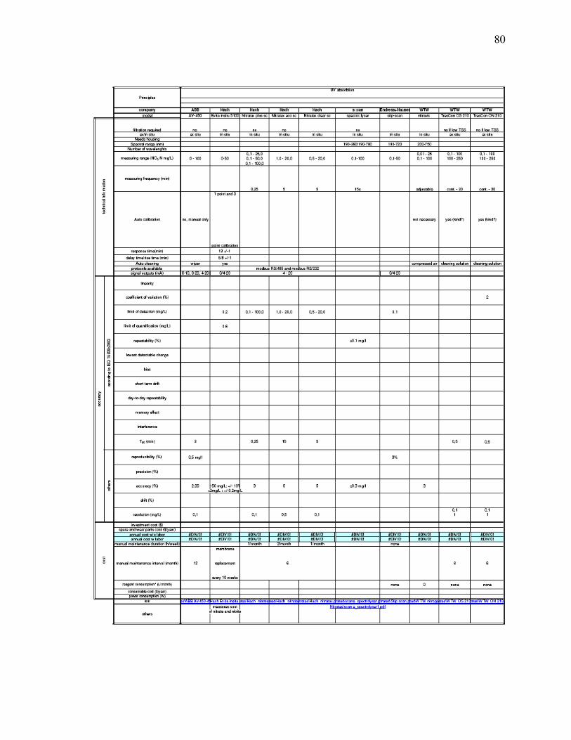
80
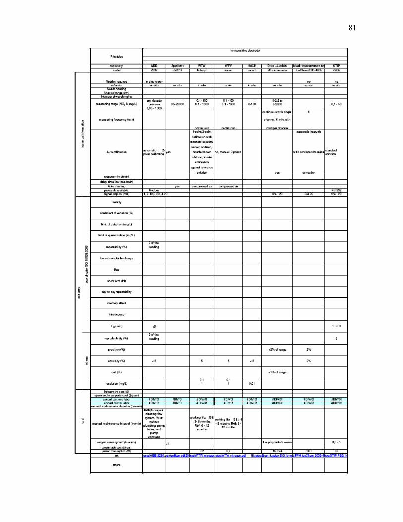
81
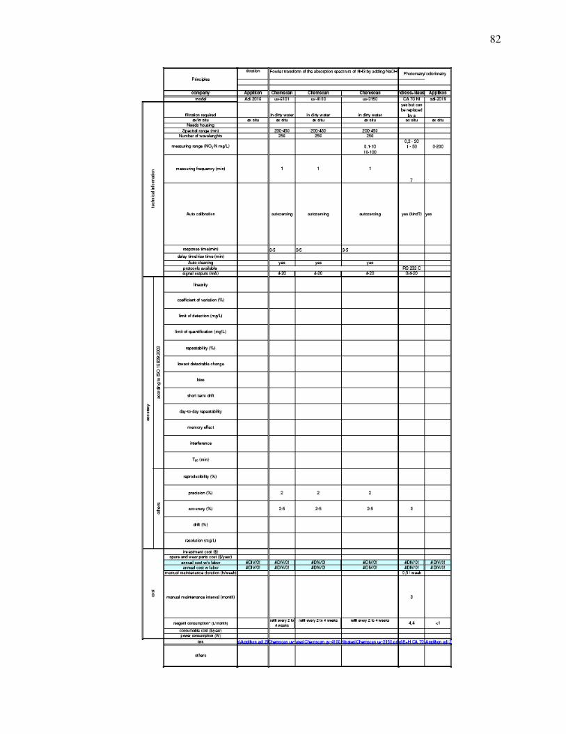
82

ANNEX B
SENSORS REVIEW TABLES – NITRITE
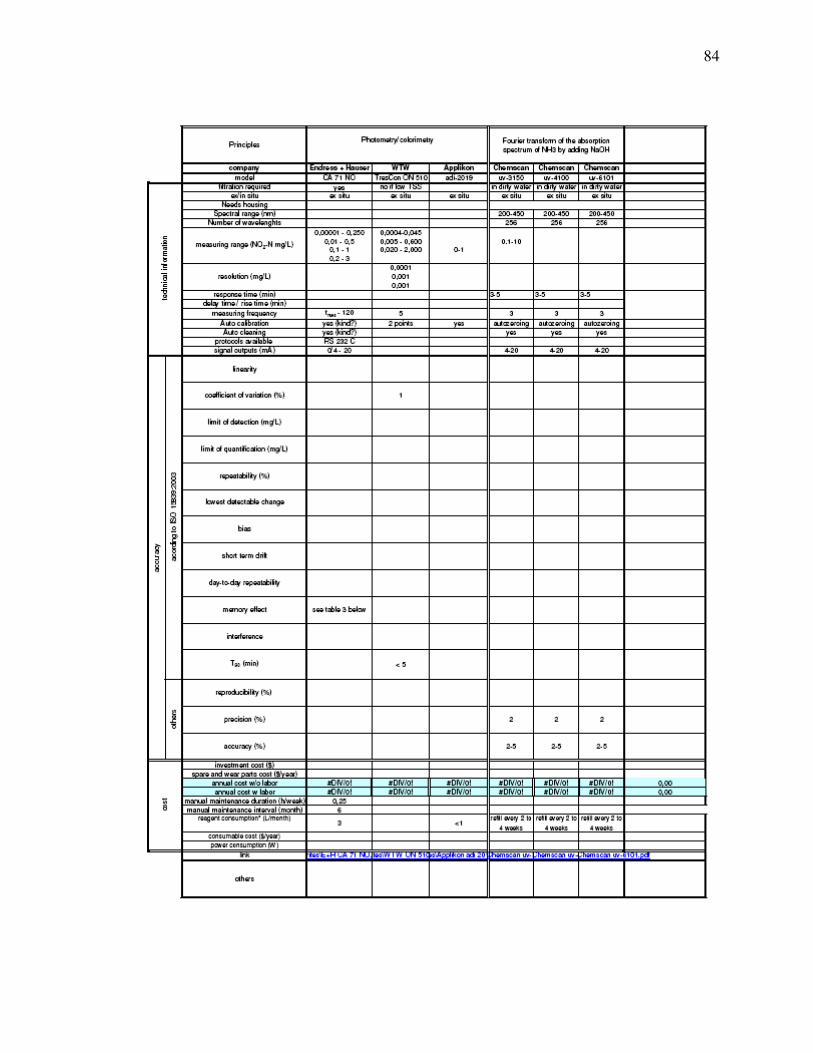
84
ANNEX C
SENSORS REVIEW TABLES - AMMONIUM
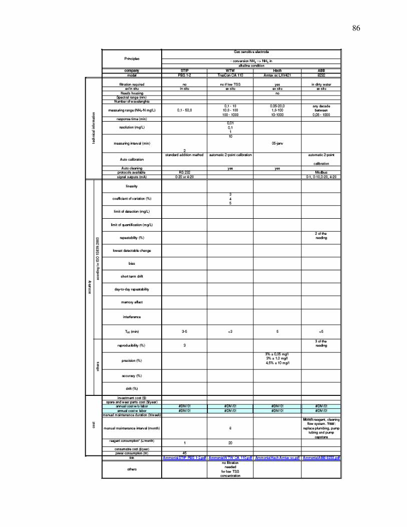
86
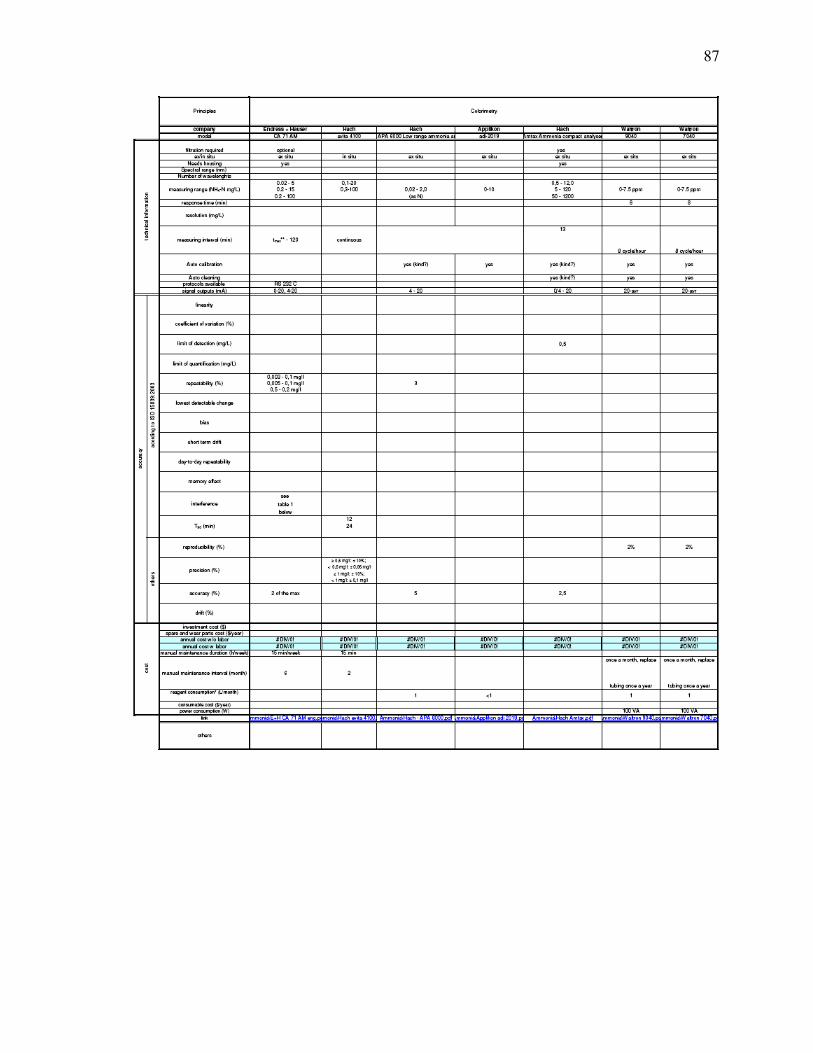
87
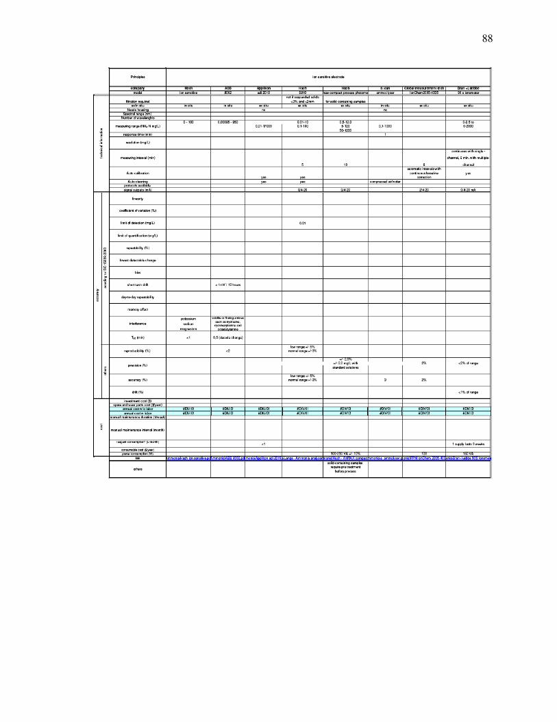
88
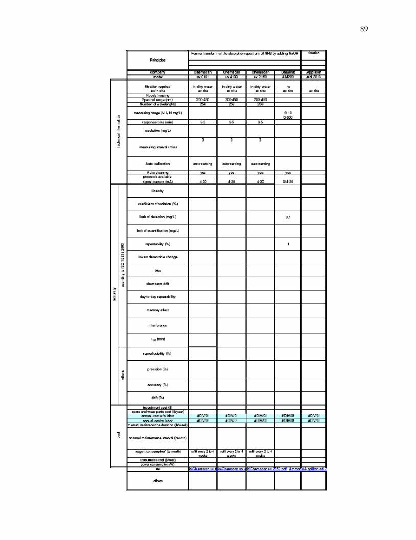
89

ANNEX D
SENSORS REVIEW TABLES – PHOSPHATE
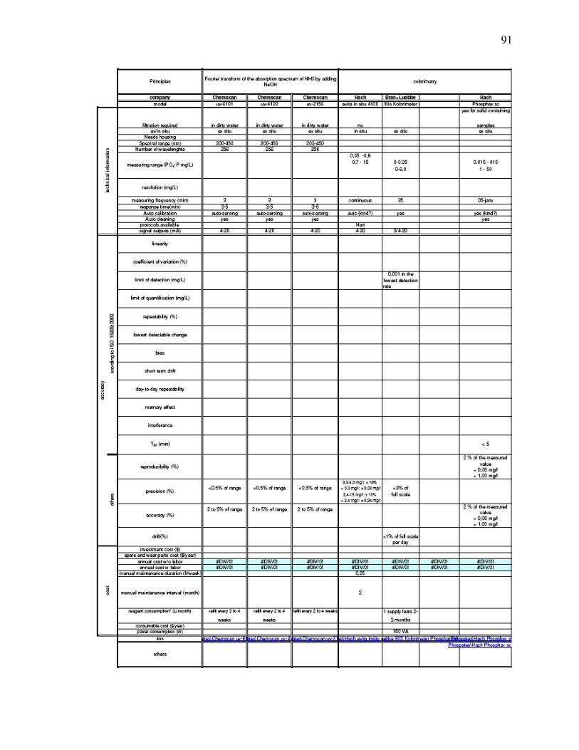
91
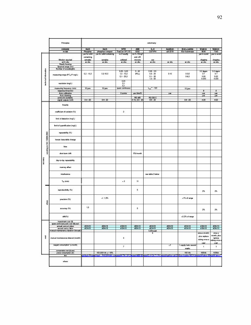
92
ANNEX E
SENSORS REVIEW TABLES – TURIDITY
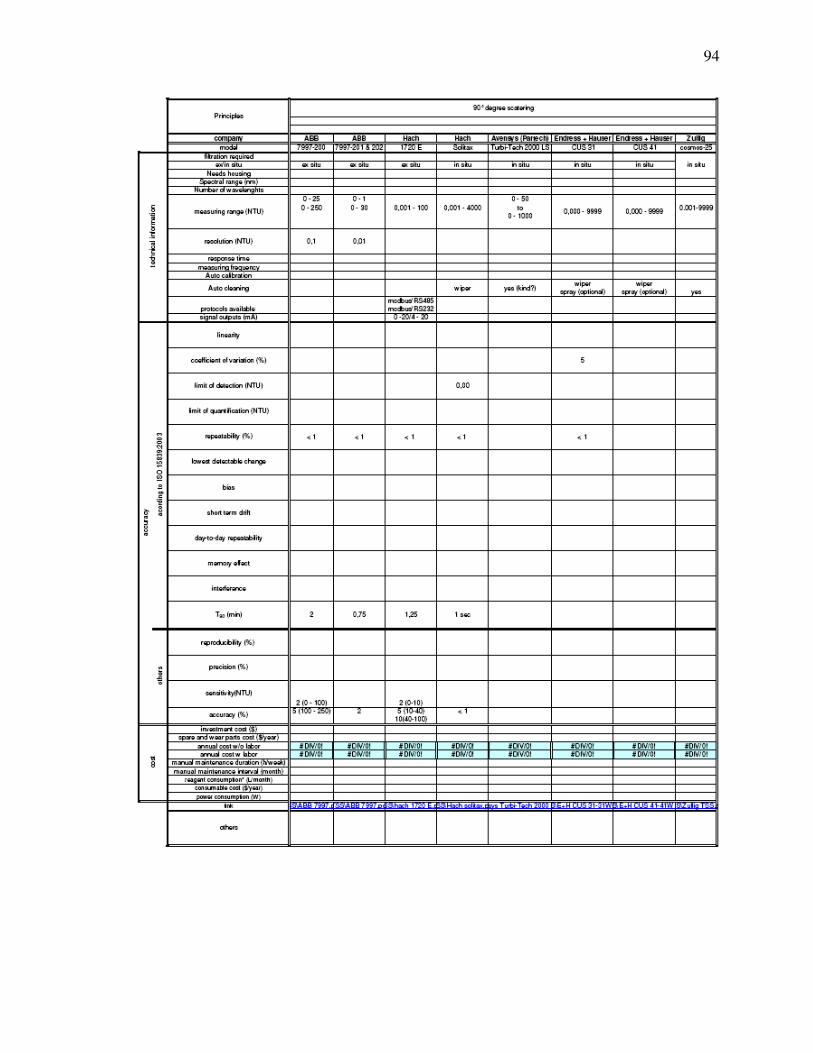
94
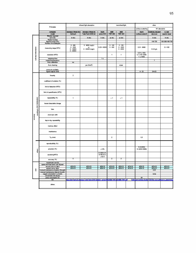
95
ANNEX F
SENSORS REVIEW TABLES – DISLOVED OXYGEN
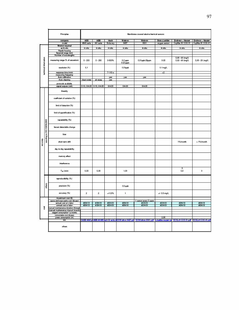
97
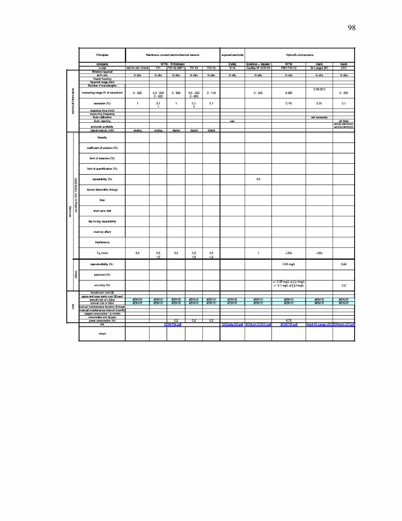
98
ANNEX G
RAW DATA – ISO 15839:2003 TESTS
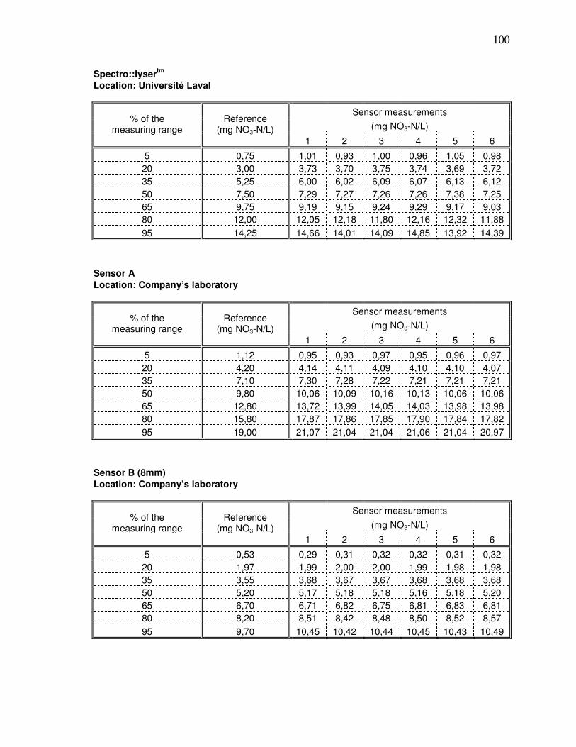
100
Spectro::lysertm
Location: Université Laval
Sensor measurements
(mg NO3-N/L) % of the
measuring range Reference
(mg NO3-N/L)
1 2 3 4 5 6
5 0,75 1,01 0,93 1,00 0,96 1,05 0,98
20 3,00 3,73 3,70 3,75 3,74 3,69 3,72
35 5,25 6,00 6,02 6,09 6,07 6,13 6,12
50 7,50 7,29 7,27 7,26 7,26 7,38 7,25
65 9,75 9,19 9,15 9,24 9,29 9,17 9,03
80 12,00 12,05 12,18 11,80 12,16 12,32 11,88
95 14,25 14,66 14,01 14,09 14,85 13,92 14,39
Sensor A
Location: Company’s laboratory
Sensor measurements
(mg NO3-N/L) % of the
measuring range Reference
(mg NO3-N/L)
1 2 3 4 5 6
5 1,12 0,95 0,93 0,97 0,95 0,96 0,97
20 4,20 4,14 4,11 4,09 4,10 4,10 4,07
35 7,10 7,30 7,28 7,22 7,21 7,21 7,21
50 9,80 10,06 10,09 10,16 10,13 10,06 10,06
65 12,80 13,72 13,99 14,05 14,03 13,98 13,98
80 15,80 17,87 17,86 17,85 17,90 17,84 17,82
95 19,00 21,07 21,04 21,04 21,06 21,04 20,97
Sensor B (8mm)
Location: Company’s laboratory
Sensor measurements
(mg NO3-N/L) % of the
measuring range Reference
(mg NO3-N/L)
1 2 3 4 5 6
5 0,53 0,29 0,31 0,32 0,32 0,31 0,32
20 1,97 1,99 2,00 2,00 1,99 1,98 1,98
35 3,55 3,68 3,67 3,67 3,68 3,68 3,68
50 5,20 5,17 5,18 5,18 5,16 5,18 5,20
65 6,70 6,71 6,82 6,75 6,81 6,83 6,81
80 8,20 8,51 8,42 8,48 8,50 8,52 8,57
95 9,70 10,45 10,42 10,44 10,45 10,43 10,49
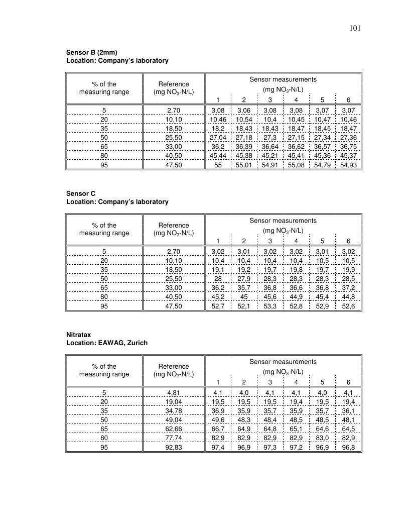
101
Sensor B (2mm)
Location: Company’s laboratory
Sensor measurements
(mg NO3-N/L) % of the
measuring range Reference
(mg NO3-N/L)
1 2 3 4 5 6
5 2,70 3,08 3,06 3,08 3,08 3,07 3,07
20 10,10 10,46 10,54 10,4 10,45 10,47 10,46
35 18,50 18,2 18,43 18,43 18,47 18,45 18,47
50 25,50 27,04 27,18 27,3 27,15 27,34 27,36
65 33,00 36,2 36,39 36,64 36,62 36,57 36,75
80 40,50 45,44 45,38 45,21 45,41 45,36 45,37
95 47,50 55 55,01 54,91 55,08 54,79 54,93
Sensor C
Location: Company’s laboratory
Sensor measurements
(mg NO3-N/L) % of the
measuring range Reference
(mg NO3-N/L)
1 2 3 4 5 6
5 2,70 3,02 3,01 3,02 3,02 3,01 3,02
20 10,10 10,4 10,4 10,4 10,4 10,5 10,5
35 18,50 19,1 19,2 19,7 19,8 19,7 19,9
50 25,50 28 27,9 28,3 28,3 28,3 28,5
65 33,00 36,2 35,7 36,8 36,6 36,8 37,2
80 40,50 45,2 45 45,6 44,9 45,4 44,8
95 47,50 52,7 52,1 53,3 52,8 52,9 52,6
Nitratax
Location: EAWAG, Zurich
Sensor measurements
(mg NO3-N/L) % of the
measuring range Reference
(mg NO3-N/L)
1 2 3 4 5 6
5 4,81 4,1 4,0 4,1 4,1 4,0 4,1
20 19,04 19,5 19,5 19,5 19,4 19,5 19,4
35 34,78 36,9 35,9 35,7 35,9 35,7 36,1
50 49,04 49,6 48,3 48,4 48,5 48,5 48,1
65 62,66 66,7 64,9 64,8 65,1 64,6 64,5
80 77,74 82,9 82,9 82,9 82,9 83,0 82,9
95 92,83 97,4 96,9 97,3 97,2 96,9 96,8
ANNEX H
RAW DATA – AIR BUBBLES TESTS
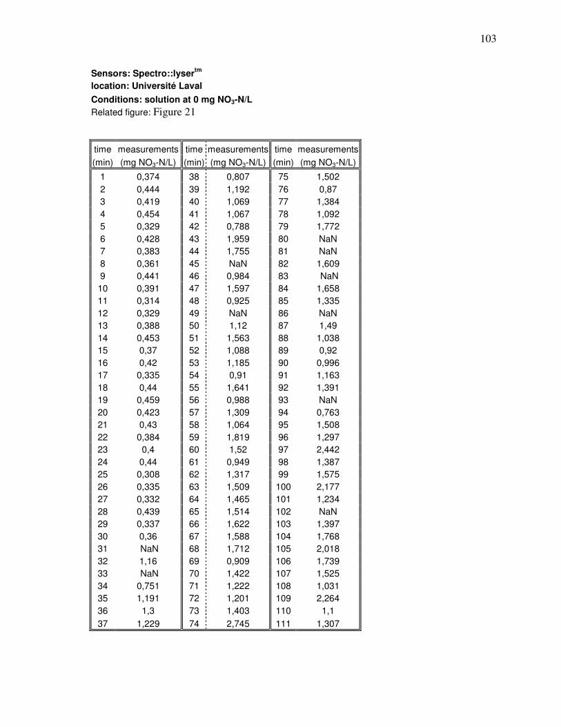
103
Sensors: Spectro::lysertm
location: Université Laval
Conditions: solution at 0 mg NO3-N/L
Related figure: Figure 21
time measurements time measurements time measurements
(min) (mg NO3-N/L) (min) (mg NO3-N/L) (min) (mg NO3-N/L)
1 0,374 38 0,807 75 1,502
2 0,444 39 1,192 76 0,87
3 0,419 40 1,069 77 1,384
4 0,454 41 1,067 78 1,092
5 0,329 42 0,788 79 1,772
6 0,428 43 1,959 80 NaN
7 0,383 44 1,755 81 NaN
8 0,361 45 NaN 82 1,609
9 0,441 46 0,984 83 NaN
10 0,391 47 1,597 84 1,658
11 0,314 48 0,925 85 1,335
12 0,329 49 NaN 86 NaN
13 0,388 50 1,12 87 1,49
14 0,453 51 1,563 88 1,038
15 0,37 52 1,088 89 0,92
16 0,42 53 1,185 90 0,996
17 0,335 54 0,91 91 1,163
18 0,44 55 1,641 92 1,391
19 0,459 56 0,988 93 NaN
20 0,423 57 1,309 94 0,763
21 0,43 58 1,064 95 1,508
22 0,384 59 1,819 96 1,297
23 0,4 60 1,52 97 2,442
24 0,44 61 0,949 98 1,387
25 0,308 62 1,317 99 1,575
26 0,335 63 1,509 100 2,177
27 0,332 64 1,465 101 1,234
28 0,439 65 1,514 102 NaN
29 0,337 66 1,622 103 1,397
30 0,36 67 1,588 104 1,768
31 NaN 68 1,712 105 2,018
32 1,16 69 0,909 106 1,739
33 NaN 70 1,422 107 1,525
34 0,751 71 1,222 108 1,031
35 1,191 72 1,201 109 2,264
36 1,3 73 1,403 110 1,1
37 1,229 74 2,745 111 1,307
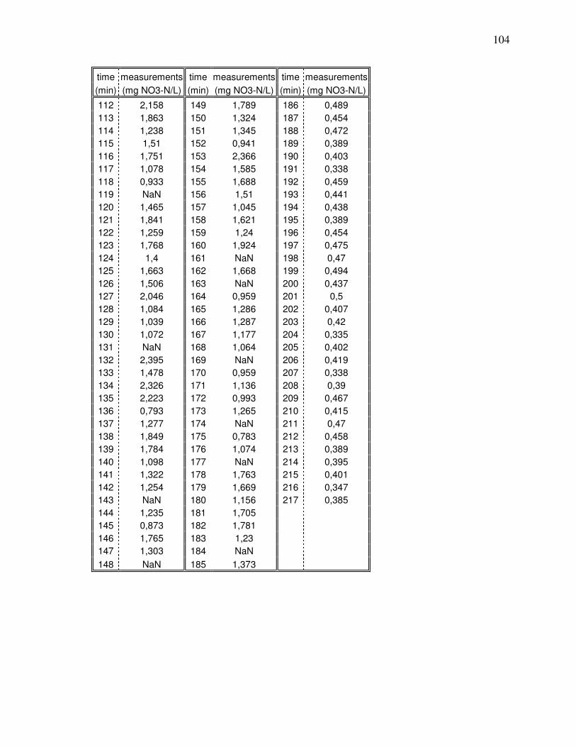
104
time measurements time measurements time measurements
(min) (mg NO3-N/L) (min) (mg NO3-N/L) (min) (mg NO3-N/L)
112 2,158 149 1,789 186 0,489
113 1,863 150 1,324 187 0,454
114 1,238 151 1,345 188 0,472
115 1,51 152 0,941 189 0,389
116 1,751 153 2,366 190 0,403
117 1,078 154 1,585 191 0,338
118 0,933 155 1,688 192 0,459
119 NaN 156 1,51 193 0,441
120 1,465 157 1,045 194 0,438
121 1,841 158 1,621 195 0,389
122 1,259 159 1,24 196 0,454
123 1,768 160 1,924 197 0,475
124 1,4 161 NaN 198 0,47
125 1,663 162 1,668 199 0,494
126 1,506 163 NaN 200 0,437
127 2,046 164 0,959 201 0,5
128 1,084 165 1,286 202 0,407
129 1,039 166 1,287 203 0,42
130 1,072 167 1,177 204 0,335
131 NaN 168 1,064 205 0,402
132 2,395 169 NaN 206 0,419
133 1,478 170 0,959 207 0,338
134 2,326 171 1,136 208 0,39
135 2,223 172 0,993 209 0,467
136 0,793 173 1,265 210 0,415
137 1,277 174 NaN 211 0,47
138 1,849 175 0,783 212 0,458
139 1,784 176 1,074 213 0,389
140 1,098 177 NaN 214 0,395
141 1,322 178 1,763 215 0,401
142 1,254 179 1,669 216 0,347
143 NaN 180 1,156 217 0,385
144 1,235 181 1,705
145 0,873 182 1,781
146 1,765 183 1,23
147 1,303 184 NaN
148 NaN 185 1,373
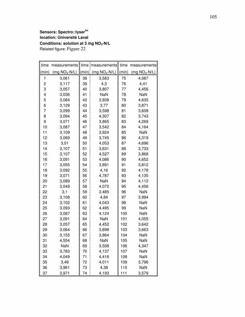
105
Sensors: Spectro::lysertm
location: Université Laval
Conditions: solution at 3 mg NO3-N/L
Related figure: Figure 22
time measurements time measurements time measurements
(min) (mg NO3-N/L) (min) (mg NO3-N/L) (min) (mg NO3-N/L)
1 3,061 38 3,583 75 4,087
2 3,117 39 4,3 76 4,41
3 3,057 40 3,807 77 4,456
4 3,036 41 NaN 78 NaN
5 3,084 42 3,938 79 4,635
6 3,129 43 3,77 80 3,871
7 3,099 44 3,598 81 3,608
8 3,094 45 4,307 82 3,743
9 3,071 46 3,865 83 4,269
10 3,087 47 3,542 84 4,164
11 3,109 48 3,924 85 NaN
12 3,069 49 3,745 86 4,319
13 3,01 50 4,053 87 4,696
14 3,107 51 3,631 88 3,733
15 3,107 52 4,527 89 3,868
16 3,091 53 4,086 90 4,652
17 3,055 54 3,891 91 3,812
18 3,092 55 4,16 92 4,178
19 3,071 56 4,787 93 4,135
20 3,089 57 NaN 94 4,112
21 3,049 58 4,072 95 4,456
22 3,1 59 3,485 96 NaN
23 3,108 60 4,84 97 3,994
24 3,102 61 4,043 98 NaN
25 3,093 62 4,495 99 NaN
26 3,087 63 4,124 100 NaN
27 3,091 64 NaN 101 4,055
28 3,057 65 4,452 102 3,642
29 3,064 66 3,898 103 3,663
30 3,155 67 3,864 104 NaN
31 4,554 68 NaN 105 NaN
32 NaN 69 3,508 106 4,347
33 3,783 70 4,137 107 NaN
34 4,049 71 4,418 108 NaN
35 3,49 72 4,011 109 3,796
36 3,961 73 4,38 110 NaN
37 3,971 74 4,193 111 3,579
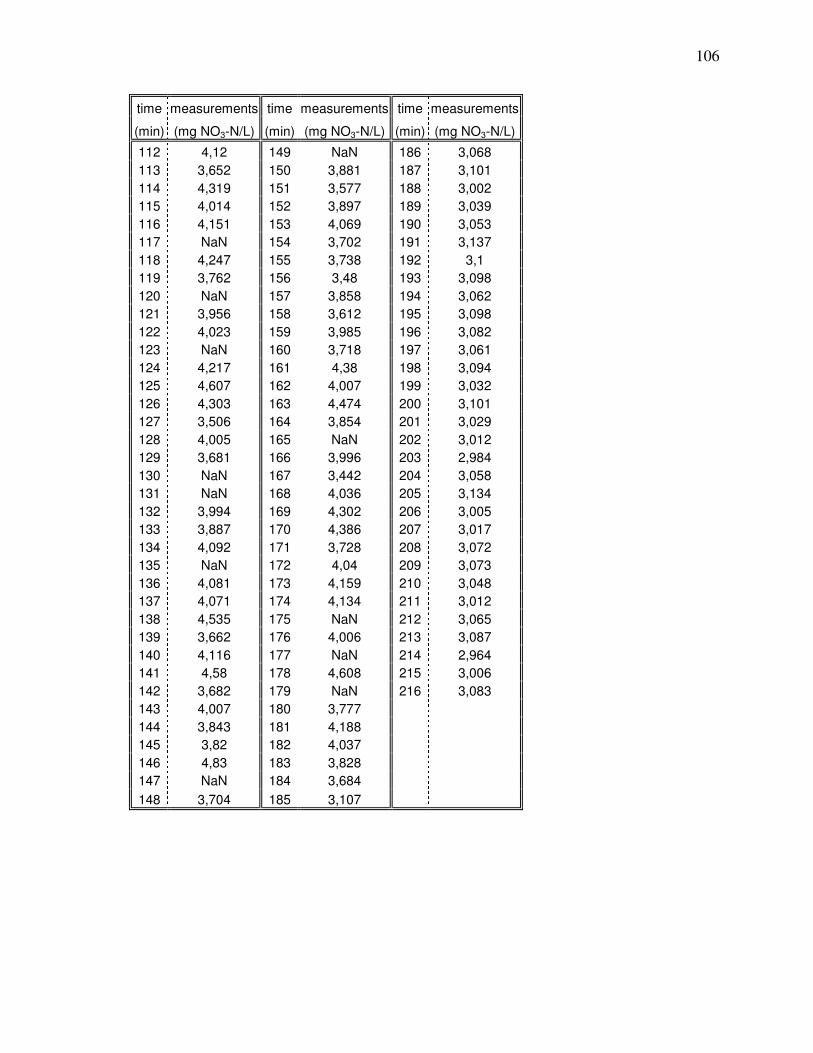
106
time measurements time measurements time measurements
(min) (mg NO3-N/L) (min) (mg NO3-N/L) (min) (mg NO3-N/L)
112 4,12 149 NaN 186 3,068
113 3,652 150 3,881 187 3,101
114 4,319 151 3,577 188 3,002
115 4,014 152 3,897 189 3,039
116 4,151 153 4,069 190 3,053
117 NaN 154 3,702 191 3,137
118 4,247 155 3,738 192 3,1
119 3,762 156 3,48 193 3,098
120 NaN 157 3,858 194 3,062
121 3,956 158 3,612 195 3,098
122 4,023 159 3,985 196 3,082
123 NaN 160 3,718 197 3,061
124 4,217 161 4,38 198 3,094
125 4,607 162 4,007 199 3,032
126 4,303 163 4,474 200 3,101
127 3,506 164 3,854 201 3,029
128 4,005 165 NaN 202 3,012
129 3,681 166 3,996 203 2,984
130 NaN 167 3,442 204 3,058
131 NaN 168 4,036 205 3,134
132 3,994 169 4,302 206 3,005
133 3,887 170 4,386 207 3,017
134 4,092 171 3,728 208 3,072
135 NaN 172 4,04 209 3,073
136 4,081 173 4,159 210 3,048
137 4,071 174 4,134 211 3,012
138 4,535 175 NaN 212 3,065
139 3,662 176 4,006 213 3,087
140 4,116 177 NaN 214 2,964
141 4,58 178 4,608 215 3,006
142 3,682 179 NaN 216 3,083
143 4,007 180 3,777
144 3,843 181 4,188
145 3,82 182 4,037
146 4,83 183 3,828
147 NaN 184 3,684
148 3,704 185 3,107
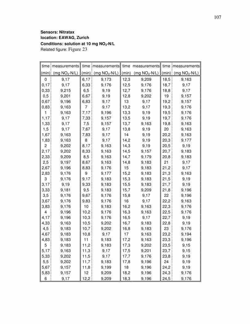
107
Sensors: Nitratax
location: EAWAG, Zurich
Conditions: solution at 10 mg NO3-N/L
Related figure: Figure 23
time measurements time measurements time measurements time measurements
(min) (mg NO3-N/L) (min) (mg NO3-N/L) (min) (mg NO3-N/L) (min) (mg NO3-N/L)
0 9,17 6,17 9,173 12,3 9,209 18,5 9,163
0,17 9,17 6,33 9,176 12,5 9,176 18,7 9,17
0,33 9,215 6,5 9,19 12,7 9,176 18,8 9,17
0,5 9,201 6,67 9,19 12,8 9,202 19 9,157
0,67 9,196 6,83 9,17 13 9,17 19,2 9,157
0,83 9,163 7 9,17 13,2 9,17 19,3 9,176
1 9,163 7,17 9,196 13,3 9,19 19,5 9,176
1,17 9,17 7,33 9,157 13,5 9,19 19,7 9,176
1,33 9,17 7,5 9,157 13,7 9,163 19,8 9,163
1,5 9,17 7,67 9,17 13,8 9,19 20 9,163
1,67 9,163 7,83 9,17 14 9,19 20,2 9,163
1,83 9,163 8 9,17 14,2 9,19 20,3 9,177
2 9,202 8,17 9,163 14,3 9,19 20,5 9,19
2,17 9,202 8,33 9,163 14,5 9,157 20,7 9,183
2,33 9,209 8,5 9,163 14,7 9,179 20,8 9,183
2,5 9,197 8,67 9,163 14,8 9,183 21 9,17
2,67 9,196 8,83 9,176 15 9,183 21,2 9,17
2,83 9,176 9 9,177 15,2 9,183 21,3 9,163
3 9,176 9,17 9,183 15,3 9,183 21,5 9,19
3,17 9,19 9,33 9,183 15,5 9,183 21,7 9,19
3,33 9,181 9,5 9,183 15,7 9,209 21,8 9,196
3,5 9,176 9,67 9,176 15,8 9,17 22 9,196
3,67 9,176 9,83 9,176 16 9,17 22,2 9,163
3,83 9,176 10 9,183 16,2 9,163 22,3 9,176
4 9,196 10,2 9,176 16,3 9,163 22,5 9,176
4,17 9,196 10,3 9,176 16,5 9,17 22,7 9,19
4,33 9,163 10,5 9,202 16,7 9,183 22,8 9,19
4,5 9,183 10,7 9,202 16,8 9,183 23 9,176
4,67 9,183 10,8 9,17 17 9,163 23,2 9,194
4,83 9,183 11 9,183 17,2 9,163 23,3 9,196
5 9,183 11,2 9,183 17,3 9,202 23,5 9,15
5,17 9,163 11,3 9,17 17,5 9,201 23,7 9,15
5,33 9,202 11,5 9,17 17,7 9,176 23,8 9,19
5,5 9,202 11,7 9,183 17,8 9,196 24 9,19
5,67 9,157 11,8 9,199 18 9,196 24,2 9,19
5,83 9,157 12 9,209 18,2 9,196 24,3 9,176
6 9,17 12,2 9,209 18,3 9,196 24,5 9,176
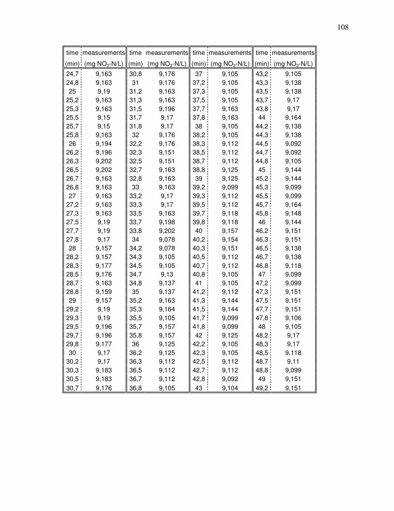
108
time measurements time measurements time measurements time measurements
(min) (mg NO3-N/L) (min) (mg NO3-N/L) (min) (mg NO3-N/L) (min) (mg NO3-N/L)
24,7 9,163 30,8 9,176 37 9,105 43,2 9,105
24,8 9,163 31 9,176 37,2 9,105 43,3 9,138
25 9,19 31,2 9,163 37,3 9,105 43,5 9,138
25,2 9,163 31,3 9,163 37,5 9,105 43,7 9,17
25,3 9,163 31,5 9,196 37,7 9,163 43,8 9,17
25,5 9,15 31,7 9,17 37,8 9,163 44 9,164
25,7 9,15 31,8 9,17 38 9,105 44,2 9,138
25,8 9,163 32 9,176 38,2 9,105 44,3 9,138
26 9,194 32,2 9,176 38,3 9,112 44,5 9,092
26,2 9,196 32,3 9,151 38,5 9,112 44,7 9,092
26,3 9,202 32,5 9,151 38,7 9,112 44,8 9,105
26,5 9,202 32,7 9,163 38,8 9,125 45 9,144
26,7 9,163 32,8 9,163 39 9,125 45,2 9,144
26,8 9,163 33 9,163 39,2 9,099 45,3 9,099
27 9,163 33,2 9,17 39,3 9,112 45,5 9,099
27,2 9,163 33,3 9,17 39,5 9,112 45,7 9,164
27,3 9,163 33,5 9,163 39,7 9,118 45,8 9,148
27,5 9,19 33,7 9,198 39,8 9,118 46 9,144
27,7 9,19 33,8 9,202 40 9,157 46,2 9,151
27,8 9,17 34 9,078 40,2 9,154 46,3 9,151
28 9,157 34,2 9,078 40,3 9,151 46,5 9,138
28,2 9,157 34,3 9,105 40,5 9,112 46,7 9,138
28,3 9,177 34,5 9,105 40,7 9,112 46,8 9,118
28,5 9,176 34,7 9,13 40,8 9,105 47 9,099
28,7 9,163 34,8 9,137 41 9,105 47,2 9,099
28,8 9,159 35 9,137 41,2 9,112 47,3 9,151
29 9,157 35,2 9,163 41,3 9,144 47,5 9,151
29,2 9,19 35,3 9,164 41,5 9,144 47,7 9,151
29,3 9,19 35,5 9,105 41,7 9,099 47,8 9,106
29,5 9,196 35,7 9,157 41,8 9,099 48 9,105
29,7 9,196 35,8 9,157 42 9,125 48,2 9,17
29,8 9,177 36 9,125 42,2 9,105 48,3 9,17
30 9,17 36,2 9,125 42,3 9,105 48,5 9,118
30,2 9,17 36,3 9,112 42,5 9,112 48,7 9,11
30,3 9,183 36,5 9,112 42,7 9,112 48,8 9,099
30,5 9,183 36,7 9,112 42,8 9,092 49 9,151
30,7 9,176 36,8 9,105 43 9,104 49,2 9,151
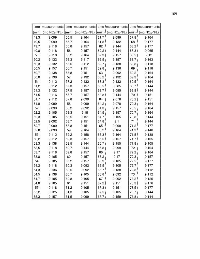
109
time measurements time measurements time measurements time measurements
(min) (mg NO3-N/L) (min) (mg NO3-N/L) (min) (mg NO3-N/L) (min) (mg NO3-N/L)
49,3 9,099 55,5 9,164 61,7 9,099 67,8 9,164
49,5 9,099 55,7 9,164 61,8 9,132 68 9,177
49,7 9,118 55,8 9,157 62 9,144 68,2 9,177
49,8 9,118 56 9,157 62,2 9,144 68,3 9,065
50 9,118 56,2 9,164 62,3 9,157 68,5 9,12
50,2 9,132 56,3 9,117 62,5 9,157 68,7 9,163
50,3 9,132 56,5 9,112 62,7 9,138 68,8 9,118
50,5 9,157 56,7 9,151 62,8 9,138 69 9,118
50,7 9,138 56,8 9,151 63 9,092 69,2 9,164
50,8 9,138 57 9,132 63,2 9,132 69,3 9,164
51 9,112 57,2 9,132 63,3 9,132 69,5 9,164
51,2 9,112 57,3 9,157 63,5 9,085 69,7 9,144
51,3 9,132 57,5 9,157 63,7 9,085 69,8 9,144
51,5 9,116 57,7 9,157 63,8 9,144 70 9,151
51,7 9,112 57,8 9,099 64 9,078 70,2 9,151
51,8 9,099 58 9,099 64,2 9,078 70,3 9,164
52 9,099 58,2 9,092 64,3 9,157 70,5 9,164
52,2 9,105 58,3 9,15 64,5 9,157 70,7 9,164
52,3 9,105 58,5 9,151 64,7 9,105 70,8 9,144
52,5 9,092 58,7 9,151 64,8 9,1 71 9,144
52,7 9,099 58,8 9,151 65 9,099 71,2 9,177
52,8 9,099 59 9,164 65,2 9,164 71,3 9,146
53 9,112 59,2 9,158 65,3 9,164 71,5 9,138
53,2 9,112 59,3 9,157 65,5 9,157 71,7 9,105
53,3 9,138 59,5 9,144 65,7 9,155 71,8 9,105
53,5 9,118 59,7 9,144 65,8 9,099 72 9,164
53,7 9,118 59,8 9,157 66 9,17 72,2 9,164
53,8 9,105 60 9,157 66,2 9,17 72,3 9,157
54 9,105 60,2 9,157 66,3 9,105 72,5 9,177
54,2 9,118 60,3 9,092 66,5 9,105 72,7 9,177
54,3 9,136 60,5 9,092 66,7 9,138 72,8 9,112
54,5 9,138 60,7 9,105 66,8 9,092 73 9,112
54,7 9,105 60,8 9,105 67 9,092 73,2 9,125
54,8 9,105 61 9,151 67,2 9,151 73,3 9,176
55 9,118 61,2 9,105 67,3 9,151 73,5 9,177
55,2 9,125 61,3 9,105 67,5 9,105 73,7 9,144
55,3 9,157 61,5 9,099 67,7 9,159 73,8 9,144
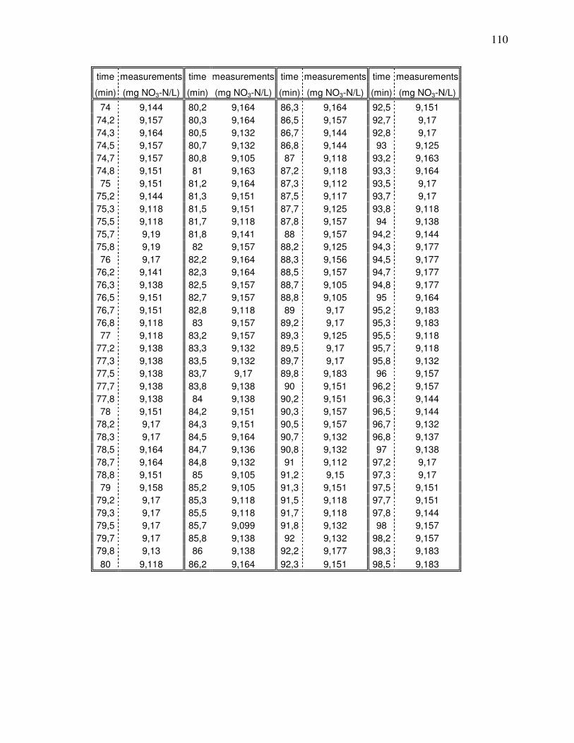
110
time measurements time measurements time measurements time measurements
(min) (mg NO3-N/L) (min) (mg NO3-N/L) (min) (mg NO3-N/L) (min) (mg NO3-N/L)
74 9,144 80,2 9,164 86,3 9,164 92,5 9,151
74,2 9,157 80,3 9,164 86,5 9,157 92,7 9,17
74,3 9,164 80,5 9,132 86,7 9,144 92,8 9,17
74,5 9,157 80,7 9,132 86,8 9,144 93 9,125
74,7 9,157 80,8 9,105 87 9,118 93,2 9,163
74,8 9,151 81 9,163 87,2 9,118 93,3 9,164
75 9,151 81,2 9,164 87,3 9,112 93,5 9,17
75,2 9,144 81,3 9,151 87,5 9,117 93,7 9,17
75,3 9,118 81,5 9,151 87,7 9,125 93,8 9,118
75,5 9,118 81,7 9,118 87,8 9,157 94 9,138
75,7 9,19 81,8 9,141 88 9,157 94,2 9,144
75,8 9,19 82 9,157 88,2 9,125 94,3 9,177
76 9,17 82,2 9,164 88,3 9,156 94,5 9,177
76,2 9,141 82,3 9,164 88,5 9,157 94,7 9,177
76,3 9,138 82,5 9,157 88,7 9,105 94,8 9,177
76,5 9,151 82,7 9,157 88,8 9,105 95 9,164
76,7 9,151 82,8 9,118 89 9,17 95,2 9,183
76,8 9,118 83 9,157 89,2 9,17 95,3 9,183
77 9,118 83,2 9,157 89,3 9,125 95,5 9,118
77,2 9,138 83,3 9,132 89,5 9,17 95,7 9,118
77,3 9,138 83,5 9,132 89,7 9,17 95,8 9,132
77,5 9,138 83,7 9,17 89,8 9,183 96 9,157
77,7 9,138 83,8 9,138 90 9,151 96,2 9,157
77,8 9,138 84 9,138 90,2 9,151 96,3 9,144
78 9,151 84,2 9,151 90,3 9,157 96,5 9,144
78,2 9,17 84,3 9,151 90,5 9,157 96,7 9,132
78,3 9,17 84,5 9,164 90,7 9,132 96,8 9,137
78,5 9,164 84,7 9,136 90,8 9,132 97 9,138
78,7 9,164 84,8 9,132 91 9,112 97,2 9,17
78,8 9,151 85 9,105 91,2 9,15 97,3 9,17
79 9,158 85,2 9,105 91,3 9,151 97,5 9,151
79,2 9,17 85,3 9,118 91,5 9,118 97,7 9,151
79,3 9,17 85,5 9,118 91,7 9,118 97,8 9,144
79,5 9,17 85,7 9,099 91,8 9,132 98 9,157
79,7 9,17 85,8 9,138 92 9,132 98,2 9,157
79,8 9,13 86 9,138 92,2 9,177 98,3 9,183
80 9,118 86,2 9,164 92,3 9,151 98,5 9,183
111
time measurements time measurements time measurements time measurements
(min) (mg NO3-N/L) (min) (mg NO3-N/L) (min) (mg NO3-N/L) (min) (mg NO3-N/L)
98,7 9,144 105 9,144 111 9,157 117 9,177
98,8 9,195 105 9,144 111 9,118 117 9,183
99 9,196 105 9,125 111 9,183 118 9,183
99,2 9,17 105 9,125 112 9,183 118 9,19
99,3 9,17 106 9,177 112 9,183 118 9,19
99,5 9,105 106 9,177 112 9,183 118 9,19
99,7 9,122 106 9,177 112 9,138 118 9,151
99,8 9,132 106 9,132 112 9,132 118 9,151
100 9,17 106 9,132 112 9,132 119 9,144
100 9,17 106 9,144 113 9,17 119 9,132
100 9,132 107 9,17 113 9,17 119 9,132
101 9,132 107 9,17 113 9,138 119 9,177
101 9,177 107 9,151 113 9,176 119 9,177
101 9,144 107 9,151 113 9,177 119 9,157
101 9,144 107 9,151 113 9,183 120 9,15
101 9,125 107 9,157 114 9,183 120 9,144
101 9,125 108 9,157 114 9,157 120 9,183
102 9,183 108 9,177 114 9,157 120 9,183
102 9,145 108 9,177 114 9,177 120 9,157
102 9,144 108 9,144 114 9,17 120 9,157
102 9,125 108 9,146 114 9,17 121 9,19
102 9,125 108 9,17 115 9,177 121 9,177
102 9,138 109 9,183 115 9,177 121 9,177
103 9,141 109 9,183 115 9,203 121 9,164
103 9,177 109 9,177 115 9,164 121 9,164
103 9,164 109 9,177 115 9,164 121 9,19
103 9,164 109 9,151 115 9,144 122 9,144
103 9,144 109 9,125 116 9,144 122 9,144
103 9,144 110 9,125 116 9,183 122 9,144
104 9,151 110 9,17 116 9,158 122 9,144
104 9,177 110 9,17 116 9,157 122 9,157
104 9,177 110 9,177 116 9,151 122 9,162
104 9,144 110 9,125 116 9,151 123 9,164
104 9,144 110 9,125 117 9,17 123 9,177
104 9,177 111 9,164 117 9,17 123 9,177
105 9,183 111 9,164 117 9,183 123 9,164
105 9,183 111 9,157 117 9,177 123 9,164
112
time measurements time measurements time measurements time measurements
(min) (mg NO3-N/L) (min) (mg NO3-N/L) (min) (mg NO3-N/L) (min) (mg NO3-N/L)
123 9,19 130 9,17 136 9,166 142 9,17
124 9,164 130 9,17 136 9,164 142 9,157
124 9,164 130 9,164 136 9,164 142 9,157
124 9,177 130 9,174 136 9,164 142 9,216
124 9,177 130 9,177 136 9,125 143 9,151
124 9,164 130 9,203 137 9,125 143 9,151
124 9,183 131 9,203 137 9,17 143 9,164
125 9,183 131 9,196 137 9,157 143 9,164
125 9,177 131 9,196 137 9,157 143 9,177
125 9,177 131 9,157 137 9,19 143 9,177
125 9,151 131 9,203 137 9,19 144 9,177
125 9,154 131 9,203 138 9,183 144 9,19
125 9,216 132 9,177 138 9,215 144 9,19
126 9,177 132 9,177 138 9,216 144 9,23
126 9,177 132 9,183 138 9,177 144 9,195
126 9,183 132 9,196 138 9,177 144 9,19
126 9,183 132 9,196 138 9,176 145 9,164
126 9,177 132 9,196 139 9,164 145 9,164
126 9,17 133 9,196 139 9,163 145 9,19
127 9,17 133 9,17 139 9,085 145 9,193
127 9,151 133 9,175 139 9,085 145 9,209
127 9,151 133 9,177 139 9,177 145 9,177
127 9,216 133 9,17 139 9,209 146 9,177
127 9,153 133 9,17 140 9,222 146 9,151
127 9,151 134 9,203 140 9,235 146 9,151
128 9,17 134 9,203 140 9,235 146 9,164
128 9,17 134 9,203 140 9,196 146 9,151
128 9,177 134 9,177 140 9,196 146 9,151
128 9,177 134 9,177 140 9,183 147 9,144
128 9,183 134 9,164 141 9,196 147 9,144
128 9,151 135 9,164 141 9,196 147 9,177
129 9,151 135 9,157 141 9,183 147 9,183
129 9,157 135 9,164 141 9,183 147 9,183
129 9,157 135 9,164 141 9,196 147 9,19
129 9,177 135 9,151 141 9,177 148 9,19
129 9,165 135 9,151 142 9,177 148 9,177
129 9,164 136 9,183 142 9,17 148 9,177
113
time measurements time measurements time measurements time measurements
(min) (mg NO3-N/L) (min) (mg NO3-N/L) (min) (mg NO3-N/L) (min) (mg NO3-N/L)
148 9,177 154 9,177 160 9,17 167 9,222
148 9,183 154 9,178 161 9,17 167 9,17
148 9,183 155 9,19 161 9,17 167 9,19
149 9,19 155 9,177 161 9,17 167 9,19
149 9,19 155 9,177 161 9,183 167 9,203
149 9,164 155 9,164 161 9,19 167 9,203
149 9,17 155 9,164 161 9,19 168 9,216
149 9,17 155 9,138 162 9,164 168 9,216
149 9,177 156 9,176 162 9,164 168 9,216
150 9,177 156 9,177 162 9,196 168 9,164
150 9,118 156 9,157 162 9,196 168 9,164
150 9,188 156 9,157 162 9,196 168 9,203
150 9,19 156 9,183 162 9,19 169 9,181
150 9,138 156 9,189 163 9,19 169 9,164
150 9,138 157 9,19 163 9,222 169 9,196
151 9,144 157 9,19 163 9,222 169 9,196
151 9,144 157 9,19 163 9,203 169 9,196
151 9,164 157 9,138 163 9,164 169 9,196
151 9,138 157 9,138 163 9,164 170 9,19
151 9,138 157 9,17 164 9,164 170 9,17
151 9,144 158 9,164 164 9,164 170 9,17
152 9,144 158 9,164 164 9,209 170 9,177
152 9,157 158 9,19 164 9,196 170 9,177
152 9,177 158 9,19 164 9,197 170 9,17
152 9,177 158 9,17 164 9,183 171 9,176
152 9,19 158 9,177 165 9,183 171 9,177
152 9,19 159 9,177 165 9,177 171 9,19
153 9,157 159 9,19 165 9,17 171 9,19
153 9,172 159 9,19 165 9,17 171 9,216
153 9,177 159 9,144 165 9,203 171 9,215
153 9,177 159 9,152 165 9,203 172 9,183
153 9,177 159 9,164 166 9,196 172 9,164
153 9,203 160 9,183 166 9,196 172 9,164
154 9,203 160 9,183 166 9,196 172 9,164
154 9,112 160 9,17 166 9,183 172 9,164
154 9,196 160 9,17 166 9,183 172 9,177
154 9,197 160 9,164 166 9,222 173 9,183
114
time measurements time measurements time measurements time measurements
(min) (mg NO3-N/L) (min) (mg NO3-N/L) (min) (mg NO3-N/L) (min) (mg NO3-N/L)
173 9,183 179 9,183 185 9,19 191 9,261
173 9,151 179 9,183 185 9,19 191 9,222
173 9,151 179 9,17 185 9,261 192 9,242
173 9,216 179 9,216 186 9,261 192 9,242
173 9,174 180 9,216 186 9,23 192 9,274
174 9,17 180 9,17 186 9,203 192 9,274
174 9,177 180 9,17 186 9,203 192 9,261
174 9,177 180 9,17 186 9,23 192 9,28
174 9,222 180 9,203 186 9,23 193 9,281
174 9,203 180 9,203 187 9,196 193 9,209
174 9,177 181 9,177 187 9,197 193 9,209
175 9,216 181 9,177 187 9,197 193 9,261
175 9,216 181 9,203 187 9,209 193 9,255
175 9,177 181 9,178 187 9,209 193 9,255
175 9,177 181 9,177 187 9,248 194 9,222
175 9,177 181 9,17 188 9,245 194 9,222
175 9,183 182 9,17 188 9,242 194 9,216
176 9,183 182 9,216 188 9,203 194 9,216
176 9,164 182 9,194 188 9,203 194 9,202
176 9,164 182 9,19 188 9,216 194 9,255
176 9,222 182 9,19 188 9,216 195 9,255
176 9,185 182 9,19 189 9,274 195 9,261
176 9,183 183 9,23 189 9,209 195 9,261
177 9,183 183 9,23 189 9,209 195 9,209
177 9,183 183 9,203 189 9,261 195 9,274
177 9,209 183 9,164 189 9,262 195 9,274
177 9,209 183 9,164 189 9,222 196 9,216
177 9,177 183 9,164 190 9,216 196 9,216
177 9,17 184 9,164 190 9,216 196 9,203
178 9,17 184 9,164 190 9,235 196 9,218
178 9,183 184 9,183 190 9,235 196 9,222
178 9,183 184 9,183 190 9,255 196 9,235
178 9,177 184 9,216 190 9,222 197 9,235
178 9,202 184 9,216 191 9,216 197 9,222
178 9,203 185 9,248 191 9,261 197 9,222
179 9,17 185 9,217 191 9,261 197 9,228
179 9,17 185 9,216 191 9,261 197 9,209
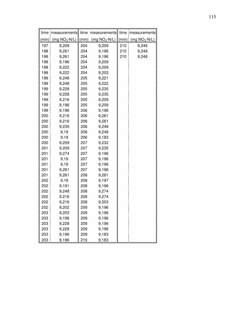
115
time measurements time measurements time measurements
(min) (mg NO3-N/L) (min) (mg NO3-N/L) (min) (mg NO3-N/L)
197 9,209 204 9,209 210 9,248
198 9,261 204 9,196 210 9,248
198 9,261 204 9,196 210 9,248
198 9,196 204 9,209
198 9,222 204 9,209
198 9,222 204 9,203
198 9,248 205 9,221
199 9,248 205 9,222
199 9,228 205 9,235
199 9,228 205 9,235
199 9,216 205 9,209
199 9,196 205 9,209
199 9,196 206 9,196
200 9,216 206 9,261
200 9,216 206 9,261
200 9,235 206 9,248
200 9,19 206 9,248
200 9,19 206 9,183
200 9,209 207 9,232
201 9,209 207 9,235
201 9,274 207 9,196
201 9,19 207 9,196
201 9,19 207 9,196
201 9,261 207 9,196
201 9,261 208 9,261
202 9,19 208 9,197
202 9,191 208 9,196
202 9,248 208 9,274
202 9,216 208 9,274
202 9,216 208 9,203
202 9,202 209 9,196
203 9,203 209 9,196
203 9,196 209 9,196
203 9,228 209 9,196
203 9,228 209 9,196
203 9,196 209 9,183
203 9,196 210 9,183
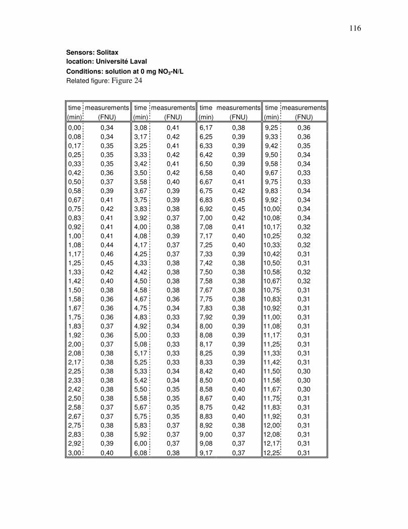
116
Sensors: Solitax
location: Université Laval
Conditions: solution at 0 mg NO3-N/L
Related figure: Figure 24
time measurements time measurements time measurements time measurements
(min) (FNU) (min) (FNU) (min) (FNU) (min) (FNU)
0,00 0,34 3,08 0,41 6,17 0,38 9,25 0,36
0,08 0,34 3,17 0,42 6,25 0,39 9,33 0,36
0,17 0,35 3,25 0,41 6,33 0,39 9,42 0,35
0,25 0,35 3,33 0,42 6,42 0,39 9,50 0,34
0,33 0,35 3,42 0,41 6,50 0,39 9,58 0,34
0,42 0,36 3,50 0,42 6,58 0,40 9,67 0,33
0,50 0,37 3,58 0,40 6,67 0,41 9,75 0,33
0,58 0,39 3,67 0,39 6,75 0,42 9,83 0,34
0,67 0,41 3,75 0,39 6,83 0,45 9,92 0,34
0,75 0,42 3,83 0,38 6,92 0,45 10,00 0,34
0,83 0,41 3,92 0,37 7,00 0,42 10,08 0,34
0,92 0,41 4,00 0,38 7,08 0,41 10,17 0,32
1,00 0,41 4,08 0,39 7,17 0,40 10,25 0,32
1,08 0,44 4,17 0,37 7,25 0,40 10,33 0,32
1,17 0,46 4,25 0,37 7,33 0,39 10,42 0,31
1,25 0,45 4,33 0,38 7,42 0,38 10,50 0,31
1,33 0,42 4,42 0,38 7,50 0,38 10,58 0,32
1,42 0,40 4,50 0,38 7,58 0,38 10,67 0,32
1,50 0,38 4,58 0,38 7,67 0,38 10,75 0,31
1,58 0,36 4,67 0,36 7,75 0,38 10,83 0,31
1,67 0,36 4,75 0,34 7,83 0,38 10,92 0,31
1,75 0,36 4,83 0,33 7,92 0,39 11,00 0,31
1,83 0,37 4,92 0,34 8,00 0,39 11,08 0,31
1,92 0,36 5,00 0,33 8,08 0,39 11,17 0,31
2,00 0,37 5,08 0,33 8,17 0,39 11,25 0,31
2,08 0,38 5,17 0,33 8,25 0,39 11,33 0,31
2,17 0,38 5,25 0,33 8,33 0,39 11,42 0,31
2,25 0,38 5,33 0,34 8,42 0,40 11,50 0,30
2,33 0,38 5,42 0,34 8,50 0,40 11,58 0,30
2,42 0,38 5,50 0,35 8,58 0,40 11,67 0,30
2,50 0,38 5,58 0,35 8,67 0,40 11,75 0,31
2,58 0,37 5,67 0,35 8,75 0,42 11,83 0,31
2,67 0,37 5,75 0,35 8,83 0,40 11,92 0,31
2,75 0,38 5,83 0,37 8,92 0,38 12,00 0,31
2,83 0,38 5,92 0,37 9,00 0,37 12,08 0,31
2,92 0,39 6,00 0,37 9,08 0,37 12,17 0,31
3,00 0,40 6,08 0,38 9,17 0,37 12,25 0,31
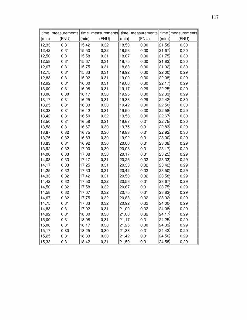
117
time measurements time measurements time measurements time measurements
(min) (FNU) (min) (FNU) (min) (FNU) (min) (FNU)
12,33 0,31 15,42 0,32 18,50 0,30 21,58 0,30
12,42 0,31 15,50 0,32 18,58 0,30 21,67 0,30
12,50 0,31 15,58 0,31 18,67 0,30 21,75 0,30
12,58 0,31 15,67 0,31 18,75 0,30 21,83 0,30
12,67 0,31 15,75 0,31 18,83 0,30 21,92 0,30
12,75 0,31 15,83 0,31 18,92 0,30 22,00 0,29
12,83 0,31 15,92 0,31 19,00 0,30 22,08 0,29
12,92 0,31 16,00 0,31 19,08 0,30 22,17 0,29
13,00 0,31 16,08 0,31 19,17 0,29 22,25 0,29
13,08 0,30 16,17 0,30 19,25 0,30 22,33 0,29
13,17 0,31 16,25 0,31 19,33 0,29 22,42 0,30
13,25 0,31 16,33 0,30 19,42 0,30 22,50 0,30
13,33 0,31 16,42 0,31 19,50 0,30 22,58 0,29
13,42 0,31 16,50 0,32 19,58 0,30 22,67 0,30
13,50 0,31 16,58 0,31 19,67 0,31 22,75 0,30
13,58 0,31 16,67 0,30 19,75 0,31 22,83 0,29
13,67 0,32 16,75 0,30 19,83 0,31 22,92 0,30
13,75 0,32 16,83 0,30 19,92 0,31 23,00 0,29
13,83 0,31 16,92 0,30 20,00 0,31 23,08 0,29
13,92 0,32 17,00 0,30 20,08 0,31 23,17 0,29
14,00 0,33 17,08 0,30 20,17 0,31 23,25 0,29
14,08 0,33 17,17 0,31 20,25 0,32 23,33 0,29
14,17 0,33 17,25 0,31 20,33 0,32 23,42 0,29
14,25 0,32 17,33 0,31 20,42 0,32 23,50 0,29
14,33 0,32 17,42 0,31 20,50 0,32 23,58 0,29
14,42 0,32 17,50 0,32 20,58 0,31 23,67 0,29
14,50 0,32 17,58 0,32 20,67 0,31 23,75 0,29
14,58 0,32 17,67 0,32 20,75 0,31 23,83 0,29
14,67 0,32 17,75 0,32 20,83 0,32 23,92 0,29
14,75 0,31 17,83 0,32 20,92 0,32 24,00 0,29
14,83 0,31 17,92 0,31 21,00 0,32 24,08 0,29
14,92 0,31 18,00 0,30 21,08 0,32 24,17 0,29
15,00 0,31 18,08 0,31 21,17 0,31 24,25 0,29
15,08 0,31 18,17 0,30 21,25 0,30 24,33 0,29
15,17 0,30 18,25 0,30 21,33 0,31 24,42 0,29
15,25 0,31 18,33 0,30 21,42 0,31 24,50 0,29
15,33 0,31 18,42 0,31 21,50 0,31 24,58 0,29
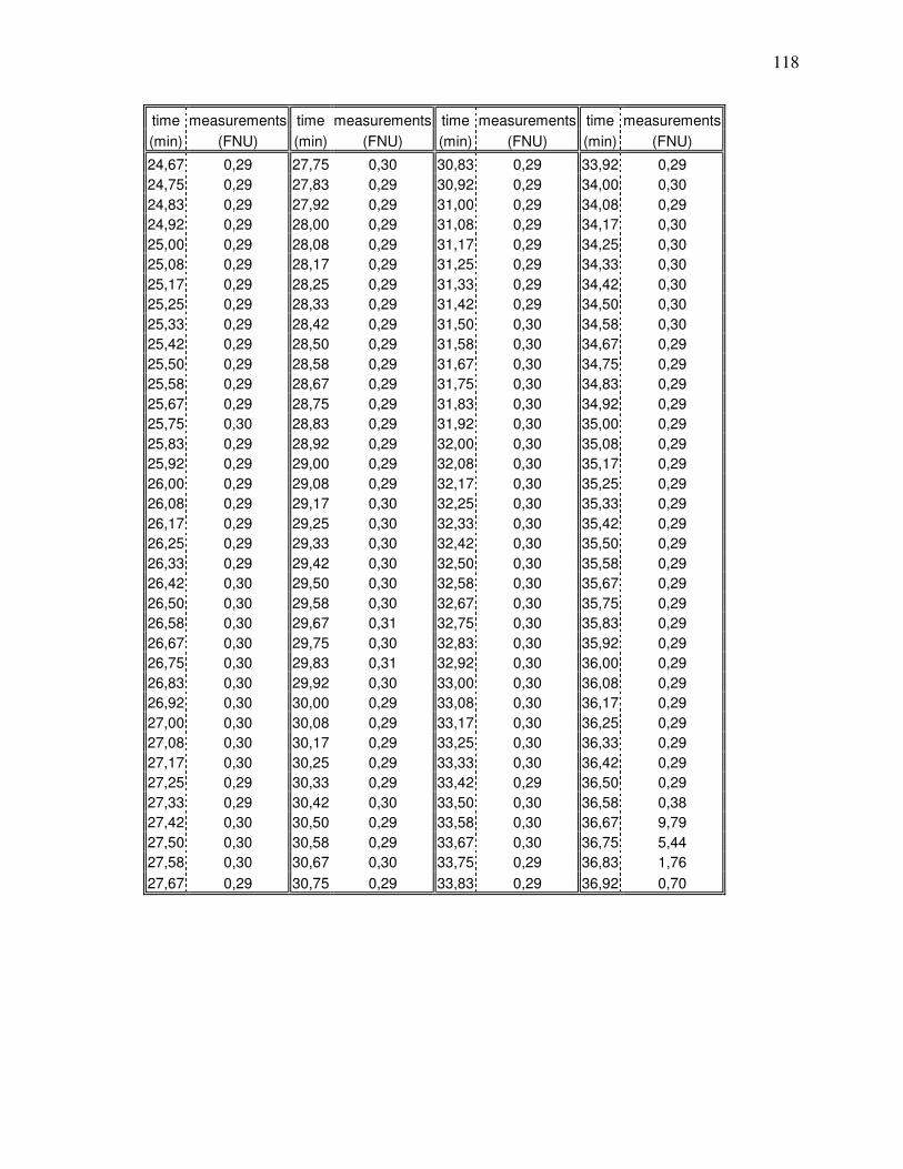
118
time measurements time measurements time measurements time measurements
(min) (FNU) (min) (FNU) (min) (FNU) (min) (FNU)
24,67 0,29 27,75 0,30 30,83 0,29 33,92 0,29
24,75 0,29 27,83 0,29 30,92 0,29 34,00 0,30
24,83 0,29 27,92 0,29 31,00 0,29 34,08 0,29
24,92 0,29 28,00 0,29 31,08 0,29 34,17 0,30
25,00 0,29 28,08 0,29 31,17 0,29 34,25 0,30
25,08 0,29 28,17 0,29 31,25 0,29 34,33 0,30
25,17 0,29 28,25 0,29 31,33 0,29 34,42 0,30
25,25 0,29 28,33 0,29 31,42 0,29 34,50 0,30
25,33 0,29 28,42 0,29 31,50 0,30 34,58 0,30
25,42 0,29 28,50 0,29 31,58 0,30 34,67 0,29
25,50 0,29 28,58 0,29 31,67 0,30 34,75 0,29
25,58 0,29 28,67 0,29 31,75 0,30 34,83 0,29
25,67 0,29 28,75 0,29 31,83 0,30 34,92 0,29
25,75 0,30 28,83 0,29 31,92 0,30 35,00 0,29
25,83 0,29 28,92 0,29 32,00 0,30 35,08 0,29
25,92 0,29 29,00 0,29 32,08 0,30 35,17 0,29
26,00 0,29 29,08 0,29 32,17 0,30 35,25 0,29
26,08 0,29 29,17 0,30 32,25 0,30 35,33 0,29
26,17 0,29 29,25 0,30 32,33 0,30 35,42 0,29
26,25 0,29 29,33 0,30 32,42 0,30 35,50 0,29
26,33 0,29 29,42 0,30 32,50 0,30 35,58 0,29
26,42 0,30 29,50 0,30 32,58 0,30 35,67 0,29
26,50 0,30 29,58 0,30 32,67 0,30 35,75 0,29
26,58 0,30 29,67 0,31 32,75 0,30 35,83 0,29
26,67 0,30 29,75 0,30 32,83 0,30 35,92 0,29
26,75 0,30 29,83 0,31 32,92 0,30 36,00 0,29
26,83 0,30 29,92 0,30 33,00 0,30 36,08 0,29
26,92 0,30 30,00 0,29 33,08 0,30 36,17 0,29
27,00 0,30 30,08 0,29 33,17 0,30 36,25 0,29
27,08 0,30 30,17 0,29 33,25 0,30 36,33 0,29
27,17 0,30 30,25 0,29 33,33 0,30 36,42 0,29
27,25 0,29 30,33 0,29 33,42 0,29 36,50 0,29
27,33 0,29 30,42 0,30 33,50 0,30 36,58 0,38
27,42 0,30 30,50 0,29 33,58 0,30 36,67 9,79
27,50 0,30 30,58 0,29 33,67 0,30 36,75 5,44
27,58 0,30 30,67 0,30 33,75 0,29 36,83 1,76
27,67 0,29 30,75 0,29 33,83 0,29 36,92 0,70
119
time measurements time measurements time measurements time measurements
(min) (FNU) (min) (FNU) (min) (FNU) (min) (FNU)
37,00 0,93 40,08 7,49 43,17 6,20 46,25 6,29
37,08 6,81 40,17 9,24 43,25 6,53 46,33 6,59
37,17 3,12 40,25 6,96 43,33 8,43 46,42 5,79
37,25 1,46 40,33 25,15 43,42 7,39 46,50 6,18
37,33 1,44 40,42 7,54 43,50 3,90 46,58 3,48
37,42 1,17 40,50 3,92 43,58 3,37 46,67 74,01
37,50 1,99 40,58 8,32 43,67 6,64 46,75 17,40
37,58 3,81 40,67 10,45 43,75 6,60 46,83 4,16
37,67 2,06 40,75 8,44 43,83 3,41 46,92 1,91
37,75 4,37 40,83 4,11 43,92 5,78 47,00 6,11
37,83 3,71 40,92 2,92 44,00 3,73 47,08 4,78
37,92 1,46 41,00 11,60 44,08 9,58 47,17 9,33
38,00 2,35 41,08 4,75 44,17 10,58 47,25 6,17
38,08 20,62 41,17 2,97 44,25 4,00 47,33 5,04
38,17 8,99 41,25 7,38 44,33 7,96 47,42 11,69
38,25 7,63 41,33 5,00 44,42 4,26 47,50 6,43
38,33 5,38 41,42 3,78 44,50 8,08 47,58 9,21
38,42 7,20 41,50 3,38 44,58 9,55 47,67 5,27
38,50 13,35 41,58 4,55 44,67 9,78 47,75 6,46
38,58 6,44 41,67 4,97 44,75 5,82 47,83 3,24
38,67 4,67 41,75 6,62 44,83 5,87 47,92 7,45
38,75 4,70 41,83 6,05 44,92 3,51 48,00 4,72
38,83 3,54 41,92 8,54 45,00 8,99 48,08 11,47
38,92 13,55 42,00 4,09 45,08 4,72 48,17 6,41
39,00 4,36 42,08 8,20 45,17 5,83 48,25 4,74
39,08 6,88 42,17 7,68 45,25 8,41 48,33 5,62
39,17 4,29 42,25 7,75 45,33 8,80 48,42 5,13
39,25 4,91 42,33 6,32 45,42 5,16 48,50 6,80
39,33 5,19 42,42 11,33 45,50 3,25 48,58 5,97
39,42 4,09 42,50 9,60 45,58 6,64 48,67 5,09
39,50 9,17 42,58 5,80 45,67 6,35 48,75 1,95
39,58 21,01 42,67 4,31 45,75 3,90 48,83 4,09
39,67 12,60 42,75 2,12 45,83 6,76 48,92 3,69
39,75 5,25 42,83 8,06 45,92 5,18 49,00 2,59
39,83 6,75 42,92 3,50 46,00 3,42 49,08 5,01
39,92 9,85 43,00 3,59 46,08 5,71 49,17 9,28
40,00 6,31 43,08 6,35 46,17 4,74 49,25 3,34
120
time measurements time measurements time measurements time measurements
(min) (FNU) (min) (FNU) (min) (FNU) (min) (FNU)
49,33 7,21 52,42 6,36 55,50 5,70 58,58 73,18
49,42 3,72 52,50 5,59 55,58 2,40 58,67 15,56
49,50 6,66 52,58 7,43 55,67 6,06 58,75 13,72
49,58 5,28 52,67 6,86 55,75 4,05 58,83 8,85
49,67 5,20 52,75 10,21 55,83 3,68 58,92 13,03
49,75 8,76 52,83 8,30 55,92 4,63 59,00 7,25
49,83 11,13 52,92 6,76 56,00 6,02 59,08 5,58
49,92 8,58 53,00 46,76 56,08 3,81 59,17 11,80
50,00 5,97 53,08 10,60 56,17 6,57 59,25 18,01
50,08 4,88 53,17 7,15 56,25 4,67 59,33 15,02
50,17 4,81 53,25 11,23 56,33 9,50 59,42 12,30
50,25 9,44 53,33 10,52 56,42 7,11 59,50 12,03
50,33 6,37 53,42 6,63 56,50 9,69 59,58 8,68
50,42 34,27 53,50 5,08 56,58 6,87 59,67 5,03
50,50 14,07 53,58 9,67 56,67 12,38 59,75 4,72
50,58 8,47 53,67 17,82 56,75 7,88 59,83 5,93
50,67 8,89 53,75 11,54 56,83 4,40 59,92 6,64
50,75 7,96 53,83 11,04 56,92 5,94 60,00 5,68
50,83 4,44 53,92 8,71 57,00 3,43 60,08 11,55
50,92 4,45 54,00 2,14 57,08 5,69 60,17 8,71
51,00 11,62 54,08 11,71 57,17 7,10 60,25 5,47
51,08 14,43 54,17 13,49 57,25 10,54 60,33 12,27
51,17 13,55 54,25 9,44 57,33 7,65 60,42 6,52
51,25 10,59 54,33 6,54 57,42 5,17 60,50 9,38
51,33 9,00 54,42 9,17 57,50 7,46 60,58 9,99
51,42 6,69 54,50 9,64 57,58 10,41 60,67 8,88
51,50 13,25 54,58 10,05 57,67 7,52 60,75 8,16
51,58 6,84 54,67 7,40 57,75 6,82 60,83 14,51
51,67 7,21 54,75 11,67 57,83 8,31 60,92 15,46
51,75 10,53 54,83 8,79 57,92 11,25 61,00 9,73
51,83 7,47 54,92 9,69 58,00 6,71 61,08 8,19
51,92 6,87 55,00 7,15 58,08 4,43 61,17 21,91
52,00 5,47 55,08 13,23 58,17 3,13 61,25 9,17
52,08 3,42 55,17 8,75 58,25 3,78 61,33 4,82
52,17 4,75 55,25 8,06 58,33 9,22 61,42 10,45
52,25 7,63 55,33 6,79 58,42 7,70 61,50 10,80
52,33 7,60 55,42 8,76 58,50 7,40 61,58 11,18
121
time measurements time measurements time measurements time measurements
(min) (FNU) (min) (FNU) (min) (FNU) (min) (FNU)
61,67 10,33 64,75 6,48 67,83 8,38 70,92 9,97
61,75 10,31 64,83 17,69 67,92 10,52 71,00 13,56
61,83 9,52 64,92 13,56 68,00 7,52 71,08 22,36
61,92 13,61 65,00 12,80 68,08 9,86 71,17 17,12
62,00 9,22 65,08 9,62 68,17 15,75 71,25 14,68
62,08 9,99 65,17 8,55 68,25 8,98 71,33 12,81
62,17 7,82 65,25 11,27 68,33 11,78 71,42 12,27
62,25 10,06 65,33 7,12 68,42 8,20 71,50 10,09
62,33 12,99 65,42 7,66 68,50 9,77 71,58 8,93
62,42 9,94 65,50 8,38 68,58 8,03 71,67 10,78
62,50 9,28 65,58 8,41 68,67 11,15 71,75 8,82
62,58 11,99 65,67 5,93 68,75 9,38 71,83 7,26
62,67 11,08 65,75 7,15 68,83 18,36 71,92 9,80
62,75 11,91 65,83 4,77 68,92 19,77 72,00 9,73
62,83 8,09 65,92 5,19 69,00 19,16 72,08 15,70
62,92 8,64 66,00 7,73 69,08 12,12 72,17 14,61
63,00 7,67 66,08 7,21 69,17 11,25 72,25 14,34
63,08 9,87 66,17 7,50 69,25 12,43 72,33 16,48
63,17 13,22 66,25 7,02 69,33 12,90 72,42 15,95
63,25 9,86 66,33 10,48 69,42 11,79 72,50 7,80
63,33 7,89 66,42 9,76 69,50 8,58 72,58 14,73
63,42 47,86 66,50 7,02 69,58 6,84 72,67 15,72
63,50 11,47 66,58 8,57 69,67 12,04 72,75 11,95
63,58 6,37 66,67 10,49 69,75 12,03 72,83 10,84
63,67 5,04 66,75 6,01 69,83 13,75 72,92 16,69
63,75 11,34 66,83 3,34 69,92 10,51 73,00 14,00
63,83 6,81 66,92 11,90 70,00 17,37 73,08 9,53
63,92 10,79 67,00 8,90 70,08 15,44 73,17 10,44
64,00 10,87 67,08 15,89 70,17 11,01 73,25 10,46
64,08 9,71 67,17 11,39 70,25 12,13 73,33 13,05
64,17 9,41 67,25 31,49 70,33 10,15 73,42 12,57
64,25 9,13 67,33 17,73 70,42 12,79 73,50 14,22
64,33 7,06 67,42 19,00 70,50 10,59 73,58 10,49
64,42 8,60 67,50 11,97 70,58 18,56 73,67 8,91
64,50 11,91 67,58 10,49 70,67 12,42 73,75 10,12
64,58 8,84 67,67 12,19 70,75 11,18 73,83 11,95
64,67 8,00 67,75 10,29 70,83 17,98 73,92 11,33
122
time measurements time measurements time measurements time measurements
(min) (FNU) (min) (FNU) (min) (FNU) (min) (FNU)
74,00 12,31 77,08 15,09 80,17 9,18 83,25 14,20
74,08 5,87 77,17 28,30 80,25 17,26 83,33 17,94
74,17 10,36 77,25 13,64 80,33 18,51 83,42 16,31
74,25 14,17 77,33 48,97 80,42 14,04 83,50 18,37
74,33 12,89 77,42 16,10 80,50 9,50 83,58 19,46
74,42 14,13 77,50 19,11 80,58 10,93 83,67 10,85
74,50 27,60 77,58 12,78 80,67 5,07 83,75 8,04
74,58 16,91 77,67 14,75 80,75 11,66 83,83 35,84
74,67 8,01 77,75 13,60 80,83 13,73 83,92 16,71
74,75 7,80 77,83 11,45 80,92 10,89 84,00 9,52
74,83 12,56 77,92 13,74 81,00 32,72 84,08 6,79
74,92 11,81 78,00 12,75 81,08 13,87 84,17 53,36
75,00 17,61 78,08 13,91 81,17 9,69 84,25 18,86
75,08 10,47 78,17 16,98 81,25 16,16 84,33 10,72
75,17 12,28 78,25 12,35 81,33 28,94 84,42 16,53
75,25 16,87 78,33 25,45 81,42 17,24 84,50 16,27
75,33 9,70 78,42 11,82 81,50 12,14 84,58 21,49
75,42 12,09 78,50 14,66 81,58 12,64 84,67 14,59
75,50 15,40 78,58 11,46 81,67 17,50 84,75 11,67
75,58 11,05 78,67 14,23 81,75 11,39 84,83 11,47
75,67 12,84 78,75 12,44 81,83 14,88 84,92 13,15
75,75 15,19 78,83 11,50 81,92 13,44 85,00 13,08
75,83 14,88 78,92 11,41 82,00 8,73 85,08 14,85
75,92 9,98 79,00 11,70 82,08 46,81 85,17 14,46
76,00 15,36 79,08 12,17 82,17 14,15 85,25 12,36
76,08 6,56 79,17 11,19 82,25 10,59 85,33 13,79
76,17 11,70 79,25 16,77 82,33 15,01 85,42 14,92
76,25 13,74 79,33 11,79 82,42 14,91 85,50 10,61
76,33 13,91 79,42 8,07 82,50 12,65 85,58 15,94
76,42 7,08 79,50 8,56 82,58 13,29 85,67 16,55
76,50 13,42 79,58 12,08 82,67 21,47 85,75 19,01
76,58 11,97 79,67 9,69 82,75 11,05 85,83 19,40
76,67 6,91 79,75 11,26 82,83 10,86 85,92 18,78
76,75 12,24 79,83 12,78 82,92 26,92 86,00 16,53
76,83 6,08 79,92 16,90 83,00 14,80 86,08 22,93
76,92 9,67 80,00 13,79 83,08 14,78 86,17 15,69
77,00 13,83 80,08 14,81 83,17 37,72 86,25 11,33
123
time measurements time measurements time measurements time measurements
(min) (FNU) (min) (FNU) (min) (FNU) (min) (FNU)
86,33 12,60 89,42 11,12 92,50 12,97 95,58 7,49
86,42 10,88 89,50 23,19 92,58 18,59 95,67 6,72
86,50 10,16 89,58 28,07 92,67 14,06 95,75 6,78
86,58 9,56 89,67 13,64 92,75 10,48 95,83 7,74
86,67 25,92 89,75 14,54 92,83 16,11 95,92 13,63
86,75 11,70 89,83 19,64 92,92 11,48 96,00 5,98
86,83 11,10 89,92 13,49 93,00 16,51 96,08 9,42
86,92 13,75 90,00 33,98 93,08 13,97 96,17 23,29
87,00 9,46 90,08 31,00 93,17 18,21 96,25 17,20
87,08 13,90 90,17 21,34 93,25 6,88 96,33 11,37
87,17 16,41 90,25 21,77 93,33 30,15 96,42 38,81
87,25 11,16 90,33 17,60 93,42 21,56 96,50 13,40
87,33 9,78 90,42 17,50 93,50 15,06 96,58 166,87
87,42 10,44 90,50 14,45 93,58 64,84 96,67 36,83
87,50 13,40 90,58 74,11 93,67 27,29 96,75 15,82
87,58 9,66 90,67 19,03 93,75 12,44 96,83 9,31
87,67 16,75 90,75 14,22 93,83 12,77 96,92 18,05
87,75 17,69 90,83 7,76 93,92 12,40 97,00 13,01
87,83 10,42 90,92 11,83 94,00 10,64 97,08 38,27
87,92 8,79 91,00 12,28 94,08 13,96 97,17 19,30
88,00 13,02 91,08 13,81 94,17 18,32 97,25 14,63
88,08 11,96 91,17 11,93 94,25 32,21 97,33 15,58
88,17 9,51 91,25 10,99 94,33 20,79 97,42 13,71
88,25 11,47 91,33 16,06 94,42 13,27 97,50 16,44
88,33 11,82 91,42 20,14 94,50 13,61 97,58 12,34
88,42 11,28 91,50 12,29 94,58 45,29 97,67 29,14
88,50 9,63 91,58 11,35 94,67 18,05 97,75 20,10
88,58 13,27 91,67 7,23 94,75 5,98 97,83 19,83
88,67 12,73 91,75 15,76 94,83 14,78 97,92 12,79
88,75 8,59 91,83 16,87 94,92 10,29 98,00 20,36
88,83 16,91 91,92 33,52 95,00 13,61 98,08 14,01
88,92 32,71 92,00 16,58 95,08 15,10 98,17 13,99
89,00 28,44 92,08 16,02 95,17 12,84 98,25 13,96
89,08 10,31 92,17 12,37 95,25 6,10 98,33 15,48
89,17 12,34 92,25 14,87 95,33 14,60 98,42 12,92
89,25 9,13 92,33 8,17 95,42 13,41 98,50 10,25
89,33 11,38 92,42 12,76 95,50 4,43 98,58 12,39
124
time measurements time measurements time measurements time measurements
(min) (FNU) (min) (FNU) (min) (FNU) (min) (FNU)
98,7 15,6 101,7 13,7 104,8 24,4 107,9 13,4
98,7 13,3 101,8 19,6 104,9 20,0 108,0 15,6
98,8 92,1 101,9 16,3 105,0 28,1 108,1 16,4
98,9 75,6 102,0 38,7 105,1 17,2 108,2 19,4
99,0 28,3 102,1 20,3 105,2 22,4 108,2 18,5
99,1 16,7 102,2 11,7 105,2 19,6 108,3 19,7
99,2 23,0 102,2 14,4 105,3 23,7 108,4 12,5
99,2 14,8 102,3 15,2 105,4 16,2 108,5 13,6
99,3 11,4 102,4 20,3 105,5 16,4 108,6 14,2
99,4 15,1 102,5 17,1 105,6 14,6 108,7 14,2
99,5 9,4 102,6 18,9 105,7 15,5 108,7 14,6
99,6 13,5 102,7 19,3 105,7 14,1 108,8 14,8
99,7 28,6 102,7 35,9 105,8 19,4 108,9 17,0
99,7 12,8 102,8 16,4 105,9 16,0 109,0 14,4
99,8 20,3 102,9 38,3 106,0 19,0 109,1 65,8
99,9 16,1 103,0 25,3 106,1 25,0 109,2 38,9
100,0 15,9 103,1 12,2 106,2 33,7 109,2 24,1
100,1 129,7 103,2 21,5 106,2 16,5 109,3 16,4
100,2 42,3 103,2 16,4 106,3 15,2 109,4 33,2
100,2 20,3 103,3 16,4 106,4 9,5 109,5 19,1
100,3 18,1 103,4 14,0 106,5 11,5 109,6 8,2
100,4 19,1 103,5 10,1 106,6 20,2 109,7 20,6
100,5 21,6 103,6 14,6 106,7 12,4 109,7 10,5
100,6 19,3 103,7 24,6 106,7 12,4 109,8 20,5
100,7 22,6 103,7 36,6 106,8 26,1 109,9 42,5
100,7 12,3 103,8 18,6 106,9 16,3 110,0 28,0
100,8 9,9 103,9 24,9 107,0 18,6 110,1 21,7
100,9 8,1 104,0 18,0 107,1 16,9 110,2 20,7
101,0 29,8 104,1 15,6 107,2 26,4 110,2 16,8
101,1 16,4 104,2 19,3 107,2 23,7 110,3 17,5
101,2 19,3 104,2 15,6 107,3 15,9 110,4 15,7
101,2 18,0 104,3 15,1 107,4 6,7 110,5 14,3
101,3 13,1 104,4 15,6 107,5 62,2 110,6 18,1
101,4 19,4 104,5 27,1 107,6 51,8 110,7 24,0
101,5 13,4 104,6 13,0 107,7 20,8 110,7 17,5
101,6 36,9 104,7 6,8 107,7 21,4 110,8 13,0
101,7 20,1 104,7 38,3 107,8 19,0 110,9 13,9
125
time measurements time measurements time measurements time measurements
(min) (FNU) (min) (FNU) (min) (FNU) (min) (FNU)
111,0 13,2 114,1 20,6 117,2 17,7 120,2 15,5
111,1 15,7 114,2 14,2 117,2 17,4 120,3 44,5
111,2 18,3 114,2 16,7 117,3 21,0 120,4 13,5
111,2 26,8 114,3 12,7 117,4 17,4 120,5 13,1
111,3 19,9 114,4 34,1 117,5 16,6 120,6 19,6
111,4 20,2 114,5 29,6 117,6 35,1 120,7 16,9
111,5 20,9 114,6 20,8 117,7 32,1 120,7 9,5
111,6 13,5 114,7 17,6 117,7 20,3 120,8 13,6
111,7 17,1 114,7 14,6 117,8 20,2 120,9 27,6
111,7 8,3 114,8 12,7 117,9 15,4 121,0 14,5
111,8 26,0 114,9 14,7 118,0 12,3 121,1 22,4
111,9 24,7 115,0 16,1 118,1 14,2 121,2 31,3
112,0 16,6 115,1 13,9 118,2 17,2 121,2 15,5
112,1 8,5 115,2 10,7 118,2 16,9 121,3 11,4
112,2 6,6 115,2 32,7 118,3 27,0 121,4 16,4
112,2 11,7 115,3 17,3 118,4 18,8 121,5 19,9
112,3 13,1 115,4 15,2 118,5 16,8 121,6 23,3
112,4 17,8 115,5 13,1 118,6 17,8 121,7 9,6
112,5 36,6 115,6 11,1 118,7 17,8 121,7 18,4
112,6 18,5 115,7 12,9 118,7 21,2 121,8 30,0
112,7 14,5 115,7 18,0 118,8 21,7 121,9 23,7
112,7 18,0 115,8 13,5 118,9 18,5 122,0 22,9
112,8 14,0 115,9 36,3 119,0 20,3 122,1 17,5
112,9 17,6 116,0 21,4 119,1 13,6 122,2 21,6
113,0 14,5 116,1 13,9 119,2 15,7 122,2 23,4
113,1 6,5 116,2 13,9 119,2 18,2 122,3 22,8
113,2 18,6 116,2 20,1 119,3 32,5 122,4 26,3
113,2 16,0 116,3 23,6 119,4 13,9 122,5 19,9
113,3 17,1 116,4 25,2 119,5 10,6 122,6 17,5
113,4 30,8 116,5 15,6 119,6 16,1 122,7 15,6
113,5 15,9 116,6 15,4 119,7 13,2 122,7 23,1
113,6 19,3 116,7 27,6 119,7 120,6 122,8 17,8
113,7 34,7 116,7 564,2 119,8 30,7 122,9 17,2
113,7 25,6 116,8 93,5 119,9 17,6 123,0 19,1
113,8 14,2 116,9 26,4 120,0 44,9 123,1 14,0
113,9 58,5 117,0 21,9 120,1 19,4 123,2 14,7
114,0 16,0 117,1 20,3 120,2 18,2 123,2 14,2
126
time measurements time measurements time measurements time measurements
(min) (FNU) (min) (FNU) (min) (FNU) (min) (FNU)
123,3 21,2 126,4 21,5 129,5 12,9 132,6 14,8
123,4 18,4 126,5 11,8 129,6 10,5 132,7 22,4
123,5 31,7 126,6 12,9 129,7 14,0 132,7 90,0
123,6 25,2 126,7 16,7 129,7 9,1 132,8 123,8
123,7 23,5 126,7 23,0 129,8 14,7 132,9 33,2
123,7 14,9 126,8 26,3 129,9 15,9 133,0 27,1
123,8 17,9 126,9 14,6 130,0 8,6 133,1 23,1
123,9 24,0 127,0 20,5 130,1 18,1 133,2 8,3
124,0 32,4 127,1 17,3 130,2 11,6 133,2 12,2
124,1 16,0 127,2 14,1 130,2 15,4 133,3 14,3
124,2 16,5 127,2 13,4 130,3 22,9 133,4 12,3
124,2 15,5 127,3 25,5 130,4 19,8 133,5 12,9
124,3 17,1 127,4 20,4 130,5 15,7 133,6 15,5
124,4 15,7 127,5 13,3 130,6 18,8 133,7 22,2
124,5 19,1 127,6 14,4 130,7 12,0 133,7 18,3
124,6 62,4 127,7 9,8 130,7 17,7 133,8 11,8
124,7 21,9 127,7 24,9 130,8 12,1 133,9 13,5
124,7 15,6 127,8 16,6 130,9 10,3 134,0 17,0
124,8 28,7 127,9 19,8 131,0 12,5 134,1 20,3
124,9 22,0 128,0 13,5 131,1 13,5 134,2 13,5
125,0 16,6 128,1 11,8 131,2 15,5 134,2 20,5
125,1 14,2 128,2 17,1 131,2 17,5 134,3 26,4
125,2 11,0 128,2 14,6 131,3 19,9 134,4 13,6
125,2 13,9 128,3 14,5 131,4 16,2 134,5 14,5
125,3 21,5 128,4 23,8 131,5 19,0 134,6 9,0
125,4 9,1 128,5 38,7 131,6 17,4 134,7 10,3
125,5 12,6 128,6 17,6 131,7 18,1 134,7 20,6
125,6 15,5 128,7 23,7 131,7 15,1 134,8 16,1
125,7 20,4 128,7 18,1 131,8 17,7 134,9 11,1
125,7 13,1 128,8 16,4 131,9 14,3 135,0 14,9
125,8 16,3 128,9 9,7 132,0 13,3 135,1 14,7
125,9 36,5 129,0 16,9 132,1 13,8 135,2 15,4
126,0 22,7 129,1 16,1 132,2 35,4 135,2 11,2
126,1 9,1 129,2 17,4 132,2 33,7 135,3 15,6
126,2 10,7 129,2 21,7 132,3 24,3 135,4 16,2
126,2 10,4 129,3 18,2 132,4 17,6 135,5 12,2
126,3 74,5 129,4 9,3 132,5 14,0 135,6 15,3
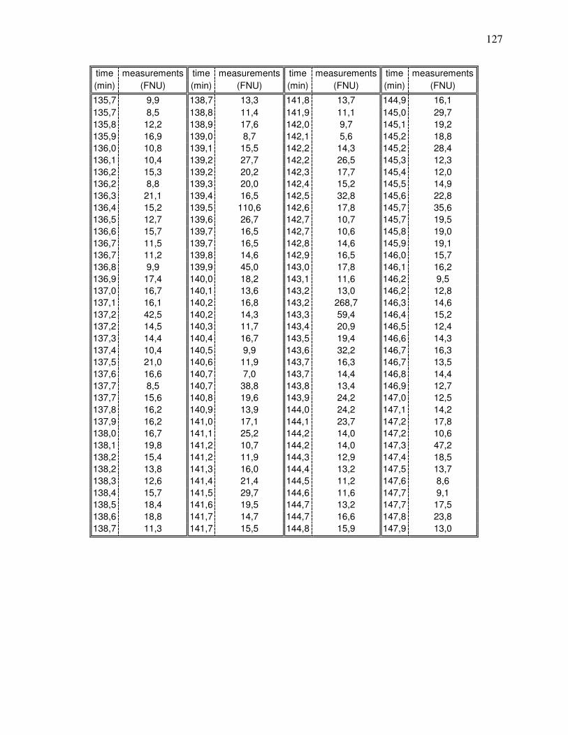
127
time measurements time measurements time measurements time measurements
(min) (FNU) (min) (FNU) (min) (FNU) (min) (FNU)
135,7 9,9 138,7 13,3 141,8 13,7 144,9 16,1
135,7 8,5 138,8 11,4 141,9 11,1 145,0 29,7
135,8 12,2 138,9 17,6 142,0 9,7 145,1 19,2
135,9 16,9 139,0 8,7 142,1 5,6 145,2 18,8
136,0 10,8 139,1 15,5 142,2 14,3 145,2 28,4
136,1 10,4 139,2 27,7 142,2 26,5 145,3 12,3
136,2 15,3 139,2 20,2 142,3 17,7 145,4 12,0
136,2 8,8 139,3 20,0 142,4 15,2 145,5 14,9
136,3 21,1 139,4 16,5 142,5 32,8 145,6 22,8
136,4 15,2 139,5 110,6 142,6 17,8 145,7 35,6
136,5 12,7 139,6 26,7 142,7 10,7 145,7 19,5
136,6 15,7 139,7 16,5 142,7 10,6 145,8 19,0
136,7 11,5 139,7 16,5 142,8 14,6 145,9 19,1
136,7 11,2 139,8 14,6 142,9 16,5 146,0 15,7
136,8 9,9 139,9 45,0 143,0 17,8 146,1 16,2
136,9 17,4 140,0 18,2 143,1 11,6 146,2 9,5
137,0 16,7 140,1 13,6 143,2 13,0 146,2 12,8
137,1 16,1 140,2 16,8 143,2 268,7 146,3 14,6
137,2 42,5 140,2 14,3 143,3 59,4 146,4 15,2
137,2 14,5 140,3 11,7 143,4 20,9 146,5 12,4
137,3 14,4 140,4 16,7 143,5 19,4 146,6 14,3
137,4 10,4 140,5 9,9 143,6 32,2 146,7 16,3
137,5 21,0 140,6 11,9 143,7 16,3 146,7 13,5
137,6 16,6 140,7 7,0 143,7 14,4 146,8 14,4
137,7 8,5 140,7 38,8 143,8 13,4 146,9 12,7
137,7 15,6 140,8 19,6 143,9 24,2 147,0 12,5
137,8 16,2 140,9 13,9 144,0 24,2 147,1 14,2
137,9 16,2 141,0 17,1 144,1 23,7 147,2 17,8
138,0 16,7 141,1 25,2 144,2 14,0 147,2 10,6
138,1 19,8 141,2 10,7 144,2 14,0 147,3 47,2
138,2 15,4 141,2 11,9 144,3 12,9 147,4 18,5
138,2 13,8 141,3 16,0 144,4 13,2 147,5 13,7
138,3 12,6 141,4 21,4 144,5 11,2 147,6 8,6
138,4 15,7 141,5 29,7 144,6 11,6 147,7 9,1
138,5 18,4 141,6 19,5 144,7 13,2 147,7 17,5
138,6 18,8 141,7 14,7 144,7 16,6 147,8 23,8
138,7 11,3 141,7 15,5 144,8 15,9 147,9 13,0
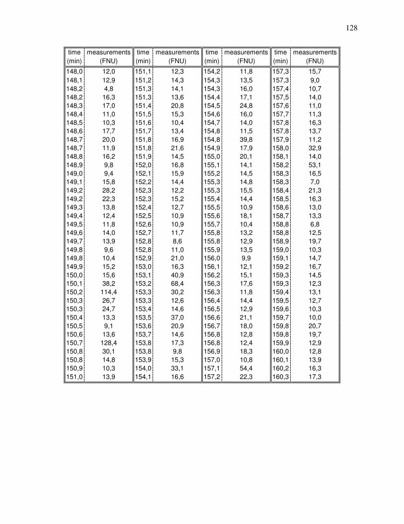
128
time measurements time measurements time measurements time measurements
(min) (FNU) (min) (FNU) (min) (FNU) (min) (FNU)
148,0 12,0 151,1 12,3 154,2 11,8 157,3 15,7
148,1 12,9 151,2 14,3 154,3 13,5 157,3 9,0
148,2 4,8 151,3 14,1 154,3 16,0 157,4 10,7
148,2 16,3 151,3 13,6 154,4 17,1 157,5 14,0
148,3 17,0 151,4 20,8 154,5 24,8 157,6 11,0
148,4 11,0 151,5 15,3 154,6 16,0 157,7 11,3
148,5 10,3 151,6 10,4 154,7 14,0 157,8 16,3
148,6 17,7 151,7 13,4 154,8 11,5 157,8 13,7
148,7 20,0 151,8 16,9 154,8 39,8 157,9 11,2
148,7 11,9 151,8 21,6 154,9 17,9 158,0 32,9
148,8 16,2 151,9 14,5 155,0 20,1 158,1 14,0
148,9 9,8 152,0 16,8 155,1 14,1 158,2 53,1
149,0 9,4 152,1 15,9 155,2 14,5 158,3 16,5
149,1 15,8 152,2 14,4 155,3 14,8 158,3 7,0
149,2 28,2 152,3 12,2 155,3 15,5 158,4 21,3
149,2 22,3 152,3 15,2 155,4 14,4 158,5 16,3
149,3 13,8 152,4 12,7 155,5 10,9 158,6 13,0
149,4 12,4 152,5 10,9 155,6 18,1 158,7 13,3
149,5 11,8 152,6 10,9 155,7 10,4 158,8 6,8
149,6 14,0 152,7 11,7 155,8 13,2 158,8 12,5
149,7 13,9 152,8 8,6 155,8 12,9 158,9 19,7
149,8 9,6 152,8 11,0 155,9 13,5 159,0 10,3
149,8 10,4 152,9 21,0 156,0 9,9 159,1 14,7
149,9 15,2 153,0 16,3 156,1 12,1 159,2 16,7
150,0 15,6 153,1 40,9 156,2 15,1 159,3 14,5
150,1 38,2 153,2 68,4 156,3 17,6 159,3 12,3
150,2 114,4 153,3 30,2 156,3 11,8 159,4 13,1
150,3 26,7 153,3 12,6 156,4 14,4 159,5 12,7
150,3 24,7 153,4 14,6 156,5 12,9 159,6 10,3
150,4 13,3 153,5 37,0 156,6 21,1 159,7 10,0
150,5 9,1 153,6 20,9 156,7 18,0 159,8 20,7
150,6 13,6 153,7 14,6 156,8 12,8 159,8 19,7
150,7 128,4 153,8 17,3 156,8 12,4 159,9 12,9
150,8 30,1 153,8 9,8 156,9 18,3 160,0 12,8
150,8 14,8 153,9 15,3 157,0 10,8 160,1 13,9
150,9 10,3 154,0 33,1 157,1 54,4 160,2 16,3
151,0 13,9 154,1 16,6 157,2 22,3 160,3 17,3
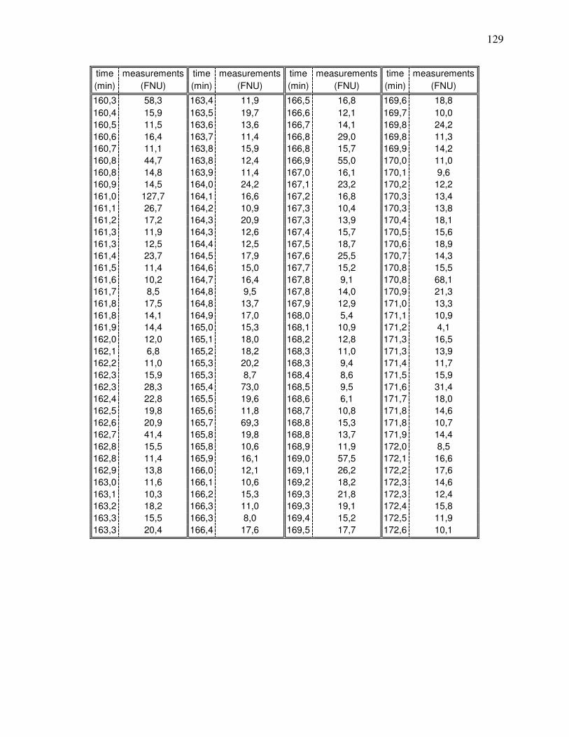
129
time measurements time measurements time measurements time measurements
(min) (FNU) (min) (FNU) (min) (FNU) (min) (FNU)
160,3 58,3 163,4 11,9 166,5 16,8 169,6 18,8
160,4 15,9 163,5 19,7 166,6 12,1 169,7 10,0
160,5 11,5 163,6 13,6 166,7 14,1 169,8 24,2
160,6 16,4 163,7 11,4 166,8 29,0 169,8 11,3
160,7 11,1 163,8 15,9 166,8 15,7 169,9 14,2
160,8 44,7 163,8 12,4 166,9 55,0 170,0 11,0
160,8 14,8 163,9 11,4 167,0 16,1 170,1 9,6
160,9 14,5 164,0 24,2 167,1 23,2 170,2 12,2
161,0 127,7 164,1 16,6 167,2 16,8 170,3 13,4
161,1 26,7 164,2 10,9 167,3 10,4 170,3 13,8
161,2 17,2 164,3 20,9 167,3 13,9 170,4 18,1
161,3 11,9 164,3 12,6 167,4 15,7 170,5 15,6
161,3 12,5 164,4 12,5 167,5 18,7 170,6 18,9
161,4 23,7 164,5 17,9 167,6 25,5 170,7 14,3
161,5 11,4 164,6 15,0 167,7 15,2 170,8 15,5
161,6 10,2 164,7 16,4 167,8 9,1 170,8 68,1
161,7 8,5 164,8 9,5 167,8 14,0 170,9 21,3
161,8 17,5 164,8 13,7 167,9 12,9 171,0 13,3
161,8 14,1 164,9 17,0 168,0 5,4 171,1 10,9
161,9 14,4 165,0 15,3 168,1 10,9 171,2 4,1
162,0 12,0 165,1 18,0 168,2 12,8 171,3 16,5
162,1 6,8 165,2 18,2 168,3 11,0 171,3 13,9
162,2 11,0 165,3 20,2 168,3 9,4 171,4 11,7
162,3 15,9 165,3 8,7 168,4 8,6 171,5 15,9
162,3 28,3 165,4 73,0 168,5 9,5 171,6 31,4
162,4 22,8 165,5 19,6 168,6 6,1 171,7 18,0
162,5 19,8 165,6 11,8 168,7 10,8 171,8 14,6
162,6 20,9 165,7 69,3 168,8 15,3 171,8 10,7
162,7 41,4 165,8 19,8 168,8 13,7 171,9 14,4
162,8 15,5 165,8 10,6 168,9 11,9 172,0 8,5
162,8 11,4 165,9 16,1 169,0 57,5 172,1 16,6
162,9 13,8 166,0 12,1 169,1 26,2 172,2 17,6
163,0 11,6 166,1 10,6 169,2 18,2 172,3 14,6
163,1 10,3 166,2 15,3 169,3 21,8 172,3 12,4
163,2 18,2 166,3 11,0 169,3 19,1 172,4 15,8
163,3 15,5 166,3 8,0 169,4 15,2 172,5 11,9
163,3 20,4 166,4 17,6 169,5 17,7 172,6 10,1
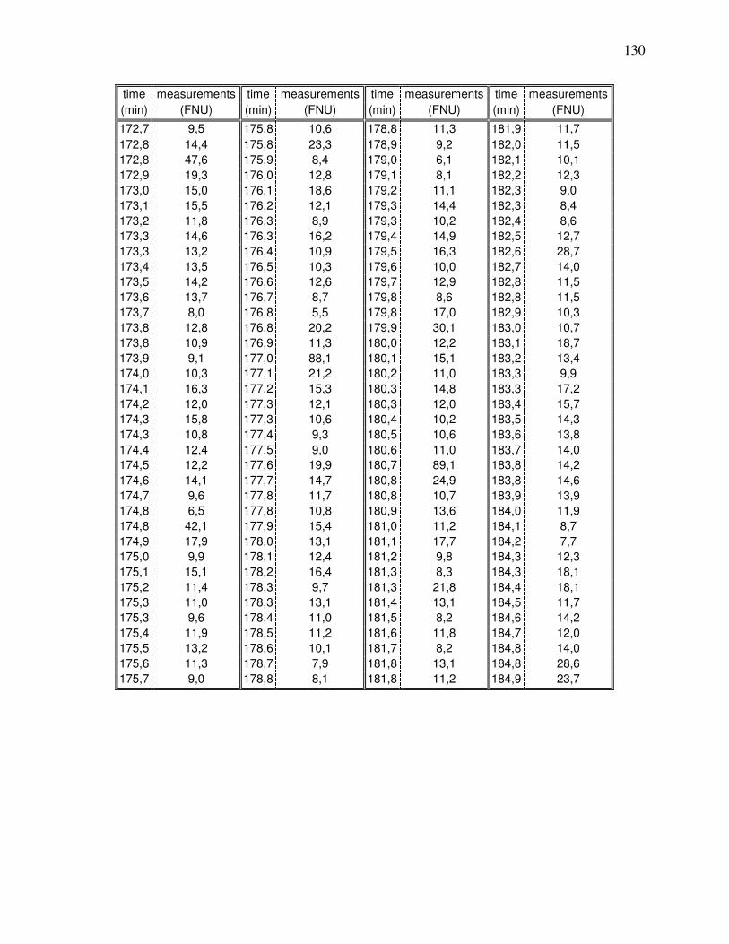
130
time measurements time measurements time measurements time measurements
(min) (FNU) (min) (FNU) (min) (FNU) (min) (FNU)
172,7 9,5 175,8 10,6 178,8 11,3 181,9 11,7
172,8 14,4 175,8 23,3 178,9 9,2 182,0 11,5
172,8 47,6 175,9 8,4 179,0 6,1 182,1 10,1
172,9 19,3 176,0 12,8 179,1 8,1 182,2 12,3
173,0 15,0 176,1 18,6 179,2 11,1 182,3 9,0
173,1 15,5 176,2 12,1 179,3 14,4 182,3 8,4
173,2 11,8 176,3 8,9 179,3 10,2 182,4 8,6
173,3 14,6 176,3 16,2 179,4 14,9 182,5 12,7
173,3 13,2 176,4 10,9 179,5 16,3 182,6 28,7
173,4 13,5 176,5 10,3 179,6 10,0 182,7 14,0
173,5 14,2 176,6 12,6 179,7 12,9 182,8 11,5
173,6 13,7 176,7 8,7 179,8 8,6 182,8 11,5
173,7 8,0 176,8 5,5 179,8 17,0 182,9 10,3
173,8 12,8 176,8 20,2 179,9 30,1 183,0 10,7
173,8 10,9 176,9 11,3 180,0 12,2 183,1 18,7
173,9 9,1 177,0 88,1 180,1 15,1 183,2 13,4
174,0 10,3 177,1 21,2 180,2 11,0 183,3 9,9
174,1 16,3 177,2 15,3 180,3 14,8 183,3 17,2
174,2 12,0 177,3 12,1 180,3 12,0 183,4 15,7
174,3 15,8 177,3 10,6 180,4 10,2 183,5 14,3
174,3 10,8 177,4 9,3 180,5 10,6 183,6 13,8
174,4 12,4 177,5 9,0 180,6 11,0 183,7 14,0
174,5 12,2 177,6 19,9 180,7 89,1 183,8 14,2
174,6 14,1 177,7 14,7 180,8 24,9 183,8 14,6
174,7 9,6 177,8 11,7 180,8 10,7 183,9 13,9
174,8 6,5 177,8 10,8 180,9 13,6 184,0 11,9
174,8 42,1 177,9 15,4 181,0 11,2 184,1 8,7
174,9 17,9 178,0 13,1 181,1 17,7 184,2 7,7
175,0 9,9 178,1 12,4 181,2 9,8 184,3 12,3
175,1 15,1 178,2 16,4 181,3 8,3 184,3 18,1
175,2 11,4 178,3 9,7 181,3 21,8 184,4 18,1
175,3 11,0 178,3 13,1 181,4 13,1 184,5 11,7
175,3 9,6 178,4 11,0 181,5 8,2 184,6 14,2
175,4 11,9 178,5 11,2 181,6 11,8 184,7 12,0
175,5 13,2 178,6 10,1 181,7 8,2 184,8 14,0
175,6 11,3 178,7 7,9 181,8 13,1 184,8 28,6
175,7 9,0 178,8 8,1 181,8 11,2 184,9 23,7
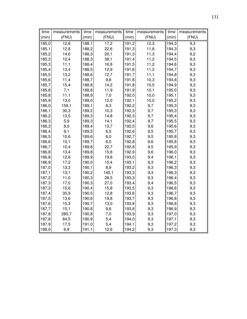
131
time measurements time measurements time measurements time measurements
(min) (FNU) (min) (FNU) (min) (FNU) (min) (FNU)
185,0 12,8 188,1 17,2 191,2 12,3 194,3 9,3
185,1 12,8 188,2 22,6 191,3 11,8 194,3 9,3
185,2 14,6 188,3 20,1 191,3 11,3 194,4 9,2
185,3 12,4 188,3 38,1 191,4 11,2 194,5 9,3
185,3 11,1 188,4 16,8 191,5 11,2 194,6 9,3
185,4 13,4 188,5 12,9 191,6 11,2 194,7 9,3
185,5 13,2 188,6 12,7 191,7 11,1 194,8 9,3
185,6 11,4 188,7 9,8 191,8 10,3 194,8 9,3
185,7 15,4 188,8 14,2 191,8 10,5 194,9 9,3
185,8 7,1 188,8 11,9 191,9 10,1 195,0 9,3
185,8 11,1 188,9 7,0 192,0 10,0 195,1 9,3
185,9 13,0 189,0 12,0 192,1 10,0 195,2 9,3
186,0 159,1 189,1 8,3 192,2 9,7 195,3 9,3
186,1 30,3 189,2 10,3 192,3 9,7 195,3 9,3
186,2 13,5 189,3 14,8 192,3 9,7 195,4 9,3
186,3 5,9 189,3 14,1 192,4 9,7 195,5 9,3
186,3 8,0 189,4 13,7 192,5 9,6 195,6 9,3
186,4 9,1 189,5 6,5 192,6 9,5 195,7 9,3
186,5 10,6 189,6 6,0 192,7 9,5 195,8 9,3
186,6 10,1 189,7 6,0 192,8 9,6 195,8 9,3
186,7 10,4 189,8 22,7 192,8 9,5 195,9 9,3
186,8 13,4 189,8 15,8 192,9 9,6 196,0 9,3
186,8 12,6 189,9 19,8 193,0 9,4 196,1 9,3
186,9 17,2 190,0 15,4 193,1 9,3 196,2 9,3
187,0 13,3 190,1 8,9 193,2 9,3 196,3 9,3
187,1 13,1 190,2 145,1 193,3 9,3 196,3 9,3
187,2 11,0 190,3 28,5 193,3 9,3 196,4 9,3
187,3 17,0 190,3 27,0 193,4 9,4 196,5 9,3
187,3 15,6 190,4 15,8 193,5 9,3 196,6 9,3
187,4 35,9 190,5 12,8 193,6 9,3 196,7 9,3
187,5 13,6 190,6 19,8 193,7 9,3 196,8 9,3
187,6 15,3 190,7 13,0 193,8 9,3 196,8 9,3
187,7 15,1 190,8 9,6 193,8 9,3 196,9 9,3
187,8 285,7 190,8 7,0 193,9 9,3 197,0 9,3
187,8 64,5 190,9 5,4 194,0 9,3 197,1 9,3
187,9 17,5 191,0 5,4 194,1 9,3 197,2 9,3
188,0 6,9 191,1 12,6 194,2 9,3 197,3 9,3
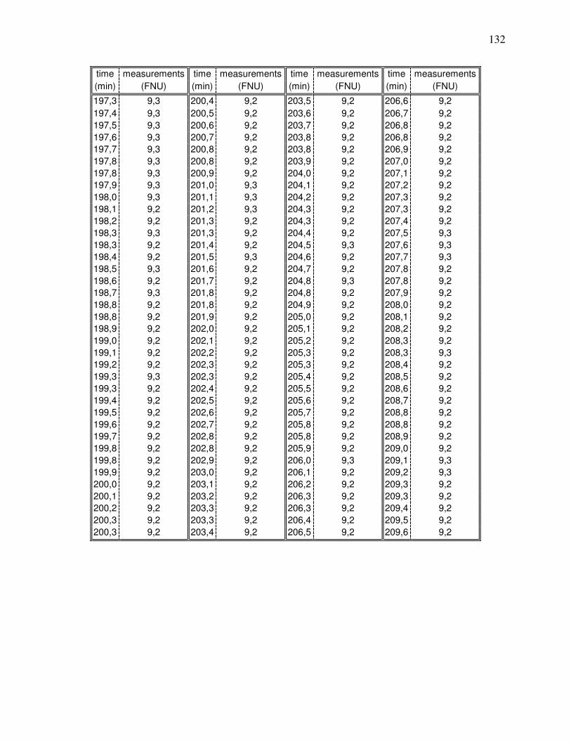
132
time measurements time measurements time measurements time measurements
(min) (FNU) (min) (FNU) (min) (FNU) (min) (FNU)
197,3 9,3 200,4 9,2 203,5 9,2 206,6 9,2
197,4 9,3 200,5 9,2 203,6 9,2 206,7 9,2
197,5 9,3 200,6 9,2 203,7 9,2 206,8 9,2
197,6 9,3 200,7 9,2 203,8 9,2 206,8 9,2
197,7 9,3 200,8 9,2 203,8 9,2 206,9 9,2
197,8 9,3 200,8 9,2 203,9 9,2 207,0 9,2
197,8 9,3 200,9 9,2 204,0 9,2 207,1 9,2
197,9 9,3 201,0 9,3 204,1 9,2 207,2 9,2
198,0 9,3 201,1 9,3 204,2 9,2 207,3 9,2
198,1 9,2 201,2 9,3 204,3 9,2 207,3 9,2
198,2 9,2 201,3 9,2 204,3 9,2 207,4 9,2
198,3 9,3 201,3 9,2 204,4 9,2 207,5 9,3
198,3 9,2 201,4 9,2 204,5 9,3 207,6 9,3
198,4 9,2 201,5 9,3 204,6 9,2 207,7 9,3
198,5 9,3 201,6 9,2 204,7 9,2 207,8 9,2
198,6 9,2 201,7 9,2 204,8 9,3 207,8 9,2
198,7 9,3 201,8 9,2 204,8 9,2 207,9 9,2
198,8 9,2 201,8 9,2 204,9 9,2 208,0 9,2
198,8 9,2 201,9 9,2 205,0 9,2 208,1 9,2
198,9 9,2 202,0 9,2 205,1 9,2 208,2 9,2
199,0 9,2 202,1 9,2 205,2 9,2 208,3 9,2
199,1 9,2 202,2 9,2 205,3 9,2 208,3 9,3
199,2 9,2 202,3 9,2 205,3 9,2 208,4 9,2
199,3 9,3 202,3 9,2 205,4 9,2 208,5 9,2
199,3 9,2 202,4 9,2 205,5 9,2 208,6 9,2
199,4 9,2 202,5 9,2 205,6 9,2 208,7 9,2
199,5 9,2 202,6 9,2 205,7 9,2 208,8 9,2
199,6 9,2 202,7 9,2 205,8 9,2 208,8 9,2
199,7 9,2 202,8 9,2 205,8 9,2 208,9 9,2
199,8 9,2 202,8 9,2 205,9 9,2 209,0 9,2
199,8 9,2 202,9 9,2 206,0 9,3 209,1 9,3
199,9 9,2 203,0 9,2 206,1 9,2 209,2 9,3
200,0 9,2 203,1 9,2 206,2 9,2 209,3 9,2
200,1 9,2 203,2 9,2 206,3 9,2 209,3 9,2
200,2 9,2 203,3 9,2 206,3 9,2 209,4 9,2
200,3 9,2 203,3 9,2 206,4 9,2 209,5 9,2
200,3 9,2 203,4 9,2 206,5 9,2 209,6 9,2
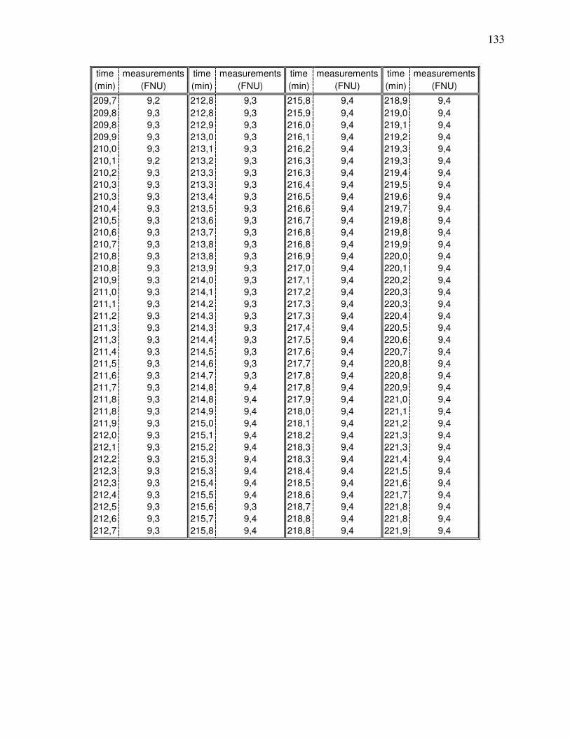
133
time measurements time measurements time measurements time measurements
(min) (FNU) (min) (FNU) (min) (FNU) (min) (FNU)
209,7 9,2 212,8 9,3 215,8 9,4 218,9 9,4
209,8 9,3 212,8 9,3 215,9 9,4 219,0 9,4
209,8 9,3 212,9 9,3 216,0 9,4 219,1 9,4
209,9 9,3 213,0 9,3 216,1 9,4 219,2 9,4
210,0 9,3 213,1 9,3 216,2 9,4 219,3 9,4
210,1 9,2 213,2 9,3 216,3 9,4 219,3 9,4
210,2 9,3 213,3 9,3 216,3 9,4 219,4 9,4
210,3 9,3 213,3 9,3 216,4 9,4 219,5 9,4
210,3 9,3 213,4 9,3 216,5 9,4 219,6 9,4
210,4 9,3 213,5 9,3 216,6 9,4 219,7 9,4
210,5 9,3 213,6 9,3 216,7 9,4 219,8 9,4
210,6 9,3 213,7 9,3 216,8 9,4 219,8 9,4
210,7 9,3 213,8 9,3 216,8 9,4 219,9 9,4
210,8 9,3 213,8 9,3 216,9 9,4 220,0 9,4
210,8 9,3 213,9 9,3 217,0 9,4 220,1 9,4
210,9 9,3 214,0 9,3 217,1 9,4 220,2 9,4
211,0 9,3 214,1 9,3 217,2 9,4 220,3 9,4
211,1 9,3 214,2 9,3 217,3 9,4 220,3 9,4
211,2 9,3 214,3 9,3 217,3 9,4 220,4 9,4
211,3 9,3 214,3 9,3 217,4 9,4 220,5 9,4
211,3 9,3 214,4 9,3 217,5 9,4 220,6 9,4
211,4 9,3 214,5 9,3 217,6 9,4 220,7 9,4
211,5 9,3 214,6 9,3 217,7 9,4 220,8 9,4
211,6 9,3 214,7 9,3 217,8 9,4 220,8 9,4
211,7 9,3 214,8 9,4 217,8 9,4 220,9 9,4
211,8 9,3 214,8 9,4 217,9 9,4 221,0 9,4
211,8 9,3 214,9 9,4 218,0 9,4 221,1 9,4
211,9 9,3 215,0 9,4 218,1 9,4 221,2 9,4
212,0 9,3 215,1 9,4 218,2 9,4 221,3 9,4
212,1 9,3 215,2 9,4 218,3 9,4 221,3 9,4
212,2 9,3 215,3 9,4 218,3 9,4 221,4 9,4
212,3 9,3 215,3 9,4 218,4 9,4 221,5 9,4
212,3 9,3 215,4 9,4 218,5 9,4 221,6 9,4
212,4 9,3 215,5 9,4 218,6 9,4 221,7 9,4
212,5 9,3 215,6 9,3 218,7 9,4 221,8 9,4
212,6 9,3 215,7 9,4 218,8 9,4 221,8 9,4
212,7 9,3 215,8 9,4 218,8 9,4 221,9 9,4
ANNEX I
RAW DATA – TURBIDITY TESTS
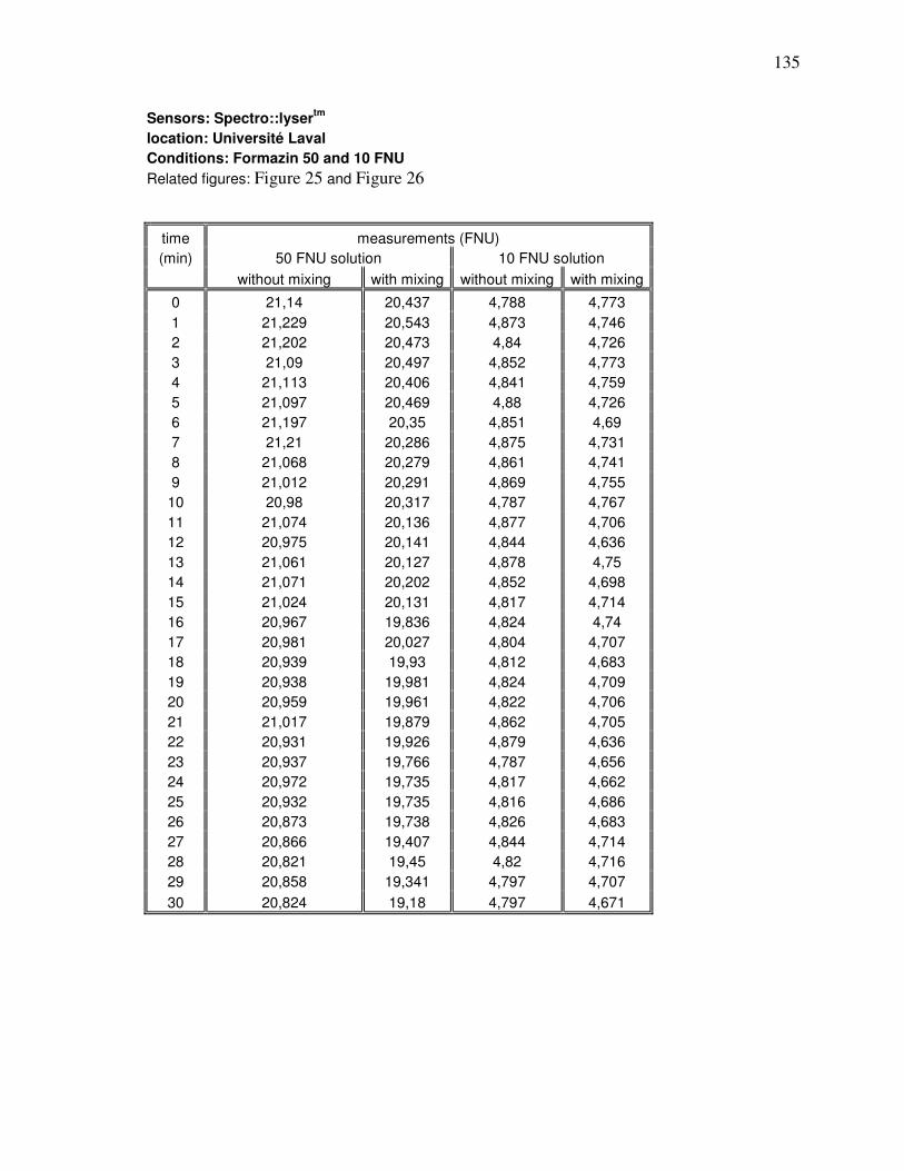
135
Sensors: Spectro::lysertm
location: Université Laval
Conditions: Formazin 50 and 10 FNU
Related figures: Figure 25 and Figure 26
time measurements (FNU)
(min) 50 FNU solution 10 FNU solution
without mixing with mixing without mixing with mixing
0 21,14 20,437 4,788 4,773
1 21,229 20,543 4,873 4,746
2 21,202 20,473 4,84 4,726
3 21,09 20,497 4,852 4,773
4 21,113 20,406 4,841 4,759
5 21,097 20,469 4,88 4,726
6 21,197 20,35 4,851 4,69
7 21,21 20,286 4,875 4,731
8 21,068 20,279 4,861 4,741
9 21,012 20,291 4,869 4,755
10 20,98 20,317 4,787 4,767
11 21,074 20,136 4,877 4,706
12 20,975 20,141 4,844 4,636
13 21,061 20,127 4,878 4,75
14 21,071 20,202 4,852 4,698
15 21,024 20,131 4,817 4,714
16 20,967 19,836 4,824 4,74
17 20,981 20,027 4,804 4,707
18 20,939 19,93 4,812 4,683
19 20,938 19,981 4,824 4,709
20 20,959 19,961 4,822 4,706
21 21,017 19,879 4,862 4,705
22 20,931 19,926 4,879 4,636
23 20,937 19,766 4,787 4,656
24 20,972 19,735 4,817 4,662
25 20,932 19,735 4,816 4,686
26 20,873 19,738 4,826 4,683
27 20,866 19,407 4,844 4,714
28 20,821 19,45 4,82 4,716
29 20,858 19,341 4,797 4,707
30 20,824 19,18 4,797 4,671
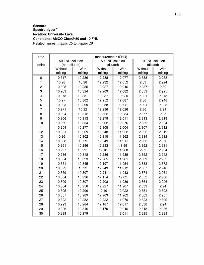
136
Sensors: Spectro::lyser
tm
location: Université Laval
Conditions: AMCO Clear® 50 and 10 FNU
Related figures: Figure 25 to Figure 29
time measurements (FNU)
(min) 50 FNU solution
(non-diluted) 50 FNU solution
(diluted) 10 FNU solution
(diluted)
Without mixing
With mixing
Without mixing
With mixing
Without mixing
With mixing
0 10,317 10,286 12,288 12,077 2,838 2,938
1 10,28 10,28 12,232 12,052 2,83 2,924
2 10,308 10,285 12,227 12,046 2,837 2,89
3 10,263 10,324 12,209 12,082 2,853 2,925
4 10,278 10,351 12,237 12,025 2,821 2,948
5 10,27 10,302 12,252 12,087 2,86 2,948
6 10,303 10,299 12,258 12,02 2,891 2,928
7 10,271 10,32 12,236 12,026 2,86 2,91
8 10,304 10,312 12,322 12,034 2,877 2,95
9 10,306 10,313 12,279 12,011 2,813 2,919
10 10,262 10,334 12,262 12,076 2,835 2,924
11 10,254 10,277 12,305 12,004 2,807 2,912
12 10,251 10,269 12,248 11,952 2,822 2,919
13 10,26 10,302 12,215 11,962 2,834 2,912
14 10,308 10,29 12,249 11,911 2,902 2,876
15 10,261 10,296 12,233 11,99 2,852 2,931
16 10,297 10,291 12,18 11,968 2,89 2,934
17 10,286 10,318 12,236 11,939 2,852 2,942
18 10,364 10,323 12,285 11,981 2,869 2,902
19 10,351 10,345 12,197 11,954 2,883 2,872
20 10,329 10,32 12,243 11,912 2,867 2,946
21 10,359 10,307 12,241 11,943 2,874 2,961
22 10,304 10,296 12,154 12,02 2,852 2,938
23 10,309 10,307 12,208 11,989 2,864 2,906
24 10,384 10,258 12,227 11,987 2,839 2,94
25 10,395 10,296 12,19 12,022 2,851 2,893
26 10,337 10,289 12,203 11,962 2,863 2,957
27 10,322 10,282 12,222 11,976 2,823 2,899
28 10,293 10,284 12,187 12,017 2,838 2,94
29 10,326 10,316 12,179 12,046 2,818 2,936
30 10,339 10,279 12,011 2,835 2,889
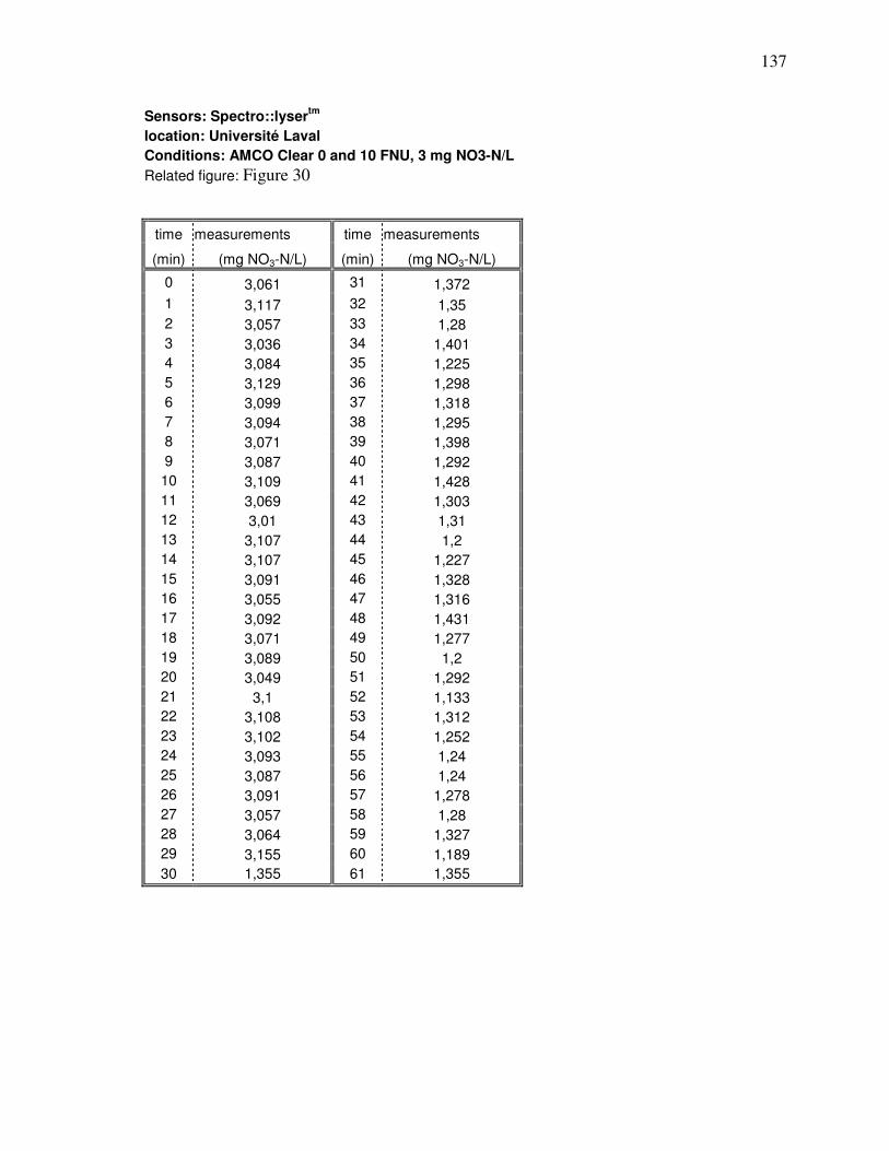
137
Sensors: Spectro::lysertm
location: Université Laval
Conditions: AMCO Clear 0 and 10 FNU, 3 mg NO3-N/L
Related figure: Figure 30
time measurements time measurements
(min) (mg NO3-N/L) (min) (mg NO3-N/L)
0 3,061 31 1,372
1 3,117 32 1,35
2 3,057 33 1,28
3 3,036 34 1,401
4 3,084 35 1,225
5 3,129 36 1,298
6 3,099 37 1,318
7 3,094 38 1,295
8 3,071 39 1,398
9 3,087 40 1,292
10 3,109 41 1,428
11 3,069 42 1,303
12 3,01 43 1,31
13 3,107 44 1,2
14 3,107 45 1,227
15 3,091 46 1,328
16 3,055 47 1,316
17 3,092 48 1,431
18 3,071 49 1,277
19 3,089 50 1,2
20 3,049 51 1,292
21 3,1 52 1,133
22 3,108 53 1,312
23 3,102 54 1,252
24 3,093 55 1,24
25 3,087 56 1,24
26 3,091 57 1,278
27 3,057 58 1,28
28 3,064 59 1,327
29 3,155 60 1,189
30 1,355 61 1,355