Centrifugal instability of pulsed...

Centrifugal instability of pulsed flow A. Aouidef Laboratoire de Physique et de Mkanique des Milieu-x H&ro@nes (PMMH)-URA CNRS N”857, Ecole Sup.&ieure de Physique et Chimie Industrielles de Paris (ESPCI), 10 rue Vauquelin, 75231 Paris Cedex 05, France

C. Normand Service de Physique Thgorique, C. E. de Saclay, 91191 Gif-sur-Yvette Cedex, France

A. Stegner and J. E. Wesfreid Laboratoire de Physique et de Mkanique des Milieux He%rog&es (PMMH)-URA CNRS N”857, Ecole Supcrieure de Physique et Chitnie Industrielles de Paris (ESPCI), 10 rue Vauquelin, 75231 Paris Cedex OS, France

(Received 8 March 1994; accepted 26 July 1994)

The stability of a pulsed flow in a Taylor-Couette geometry with both cylinders rotating at the same angular velocity fl(t)=O, cos (ot) is investigated. The first experimental evidence showing that the flow is less unstable in the limit of low and high frequency while destabilization is maximum for an intermediate frequency oO is reported. A detailed analysis of the restabilization at frequencies just above wO reveals a behavior not accounted for by previous theoretical analysis. Thus, the linear stability analysis is reconsidered by using a different implementation of the Floquet theory and a satisfactory agreement with the present experimental results is found.

I. INTRODUCTION

Hydrodynamical systems subjected to a time-dependent forcing* are encountered in several branches of fluid dynam- ics especially in relation with blood circulation and Lagrang- ian chaos. However, two problems have received special attention: the onset of convective instability in a fluid layer in the presence of a periodically varying parameter23 and the stability of a periodically modulated Taylor-Couette flow. The present study is concerned with the second of these top- ics and deals with the stability of a pulsed flow in a Taylor- Couette geometry, which is a particular case of modulated flow characterized by a zero-mean angular velocity. So we describe the pure case of a “modulation instability.”

The interest in unsteady Taylor-Couette flows was initi- ated by the experimental study of Donnelly4 where the effect of an added periodic modulation of the inner cylinder angular velocity was investigated. This early work concluded to a stabilization of the flow due to the modulation, however, the observation of “transient vortices” was reported below the onset of instability for unsteady flow. More recent experiments by Ahlers’ have shown threshold shifts above the steady onset.

The first theoretical stability analysis related to the experimental configuration of Donnelly have been formulated in the so-called narrow-gap approximation. In the limit of vanishing amplitude of the modulation and frequency, Hall6 found analytically that the threshold for onset of instability is weakly decreased from its unmodulated value. Riley and Laurence7 solved the linear equations governing the disturbance motion by a Galerkin expansion with time-dependent coefficients and then analyzed the stability of the system by the Floquet theory. Their results confirm Hall’s conclusions which suggest that modulation has a destabilizing effect.

The finite-gap range was investigated by Carmi and Tustaniwskyj* who claimed that the narrow-gap approximation is not justified in unsteady flows and possibly explain

their discrepancy with Riley and Laurence’s results about the behavior of the critical wave number as function of,the frequency when the outer cylinder is at rest and the inner cylinder rotation is modulated around a zero mean value. Carmi and Tustaniwskyj found large negative threshold shifts at low frequency of modulation which agree with Walsh and Don- nelly’s experimental findings’ who take into account the “transient vortices” for the threshold determination.

The most debated question is wether low-frequency modulation produces a large destabilization or rather a small destabilization. The latter claim was reinforced by the results of Kuhlmann et aZ.” obtained by a finite-difference numerical simulation of the full NavierStokes equations.

In their review of the literature on modulated Taylor- Couette flow, Barenghi and Jones” have also pointed out the existence of contradictory results. These authors have shown that the behavior of the flow at low frequency can be affected by very small imperfections in the apparatus that could explain the large destabilization observed in experiment. They also mentioned that a possible source of imperfections in numerical calculations arises from the choice of too large a time step in the integration of the governing equations. They suspected this is the reason why Carmi and Tustaniwskyj’ found as a result of their computations that modulation strongly destabilizes the flow.

The particular case of time-periodically driven flows in Taylor-Couette geometry with zero-mean angular velocity has only been considered in Refs. 7 and 8 with the outer cylinder at rest and in Ref. 8 for the additionnal case of both cylinders pulsating either in phase or out of phase. Recently pulsed flow was used to test Kolmogorov scaling hypothesis in the turbulent regime.‘” Closely connected to the previous configurations is the flow induced by a circular cylinder oscillating in an infinite fluid whose stability analysis was car- ried out by Seminara and Ha11.13 Unsteady Taylor-Couette flow driven by pure torsional oscillation of the entire system

Phys. Fluids 6 (ii), November 1994 1070-6631/94/6(11)/3665/12/$6.00 Q 1994 American Institute of Physics 3665

Downloaded 27 Feb 2004 to 129.199.72.5. Redistribution subject to AIP license or copyright, see http://pof.aip.org/pof/copyright.jsp

G \

I I I &--,I I I

R2 I I lb

I I I I

I I

--_ _ - - ,

FIG. 1. Sketch of the geometry.

has also been considered in the case of a two-phase system when the inner cylinder consists of a crystalline solid-liquid interface.r4

The purpose of the present paper is to investigate both experimentally and theoretically the stability of the time- periodic flow induced by two cylinders pulsating at the same frequency with equal amplitude and in the same direction. We report the first experimental observations covering a large range of frequencies. We obtain the critical values of the Taylor number and wave number as functions of the frequency. Our results reveal a new feature which was not predicted by the stability analysis of Carmi and Tustaniwskyjs likely because their stability diagram in the critical Taylor number and frequency plane was incomplete. Therefore, we perform a new stability analysis for a larger and more con- tinuous range of frequencies. The method of solving the governing differential equations for the perturbations follows the procedure formerly described in Ref. 13 and used more recently by Murray et al. I5 to study the stability of Taylor- Couette flow when the inner cylinder is rotated at a constant angular velocity and the outer cylinder is driven by a torsional oscillation about zero mean. Even though we assume the narrow-gap approximation to be valid, we obtain a stability boundary, which better agrees with our experimental results than with previous theoretical results.8

II. BASE FLOW

We consider an incompressible fluid of density p and kinematic viscosity v filling the annulus between two con- centric cylinders of radii R r and R2 = R 1 + d where d is the gap width (Fig. 1). The basic flow is driven by the motion of both cylinders rotating jointly so. that, the angular velocities of the inner and the outer cylinder, respectively a1 and a2 are equal: f12, =a2 = a. It is obvious that if the rotation is

uniform and n is constant the flow is stable. This is no longer true if the angular velocity is a time-periodic function Cl(t)=fL,+f& cos (wt) with fl, being the mean velocity, Q,a and o being respectively the amplitude and frequency of the pulsation and t the time. In the following we shall restrict attention to the special case of zero-mean angular velocity n, = 0. The case a,# 0 is analyzedI in connection with the problem of.the influence of Coriolis acceleration on centrifugal instability.‘7P’8

The governing equations are the conservation equations for momentum and mass

$+wVu=- ; VP+vAu, 0

v*u=o. (2)

In cylindrical-polar coordinates (Y, S,zj the velocity compo- nents are u=(u,u,w> in the radial, azimuthal and axial direction, respectively. Instead of the radial coordinate, we shall use the variable x defined such as r = R 1 + dx. We assume that the gap width d is small compared to the radius RI of the inner cylinder and make the small-gap approximation neglecting all terms of order d/R1 in the following. Di- mensionless variables are introduced with the scale for length,’ time and velocity being respectively d, (d’/v), R&J-

The base tlow is represented by the one-component velocity field U = (0, VB(x, t),O) where the dimensionless azimuthal velocity satisfies

av, aw, -z-=-s- 64

with the boundary conditions

v,(o,t)=V~(l,t)=cos at (3b)

where the parameter a=( od2/v) is the frequency number which is proportional to the ratio of ‘the viscous diffusive time and the period of oscillation. Associated with the base velocity is a pressure field PB(x, t) given by

JPB x-- -Vi. (4)

The solution of Eqs. (3a) and (3b) may be written as the sum of two terms

V,=V,(x)cos at+V~(x)sin at

where the functions VI and V, are given by

(5)

v,(xj=[cos (yxjcosh y(l-x)+cosh (yx)cos r(l-x)] [cash y+ cos r]

CQ:,

v 2

(x)Z[sinh (rx)sin y(l-x)+&h y(l-x)sin (yx)] [cash y+cos r]

The parameter y which is related to (T by y= m also expresses as the ratio of two lengths y=d/6 where S= J2v/w is the thickness of the Stokes layer. According to the values of u three different regimes can be observed.

3666 Phys. Fluids, Vol. 6, No. 11, November 1994 Aouidef et a/.


(a)

(bj

(cl

y= 0.8

t,=O z t1= 8 i4 t2= 4

32 t3= 8 t4= s ir

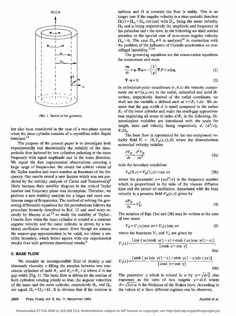
FIG. 2 Time evolution of the primary flow profile over half a period 7=27r/u for different frequencies of oscillation y. On each curve, the vertical axis is the azimuthal velocity and the horizontal one is the radial dimensionless coordinate x (x= 0 corresponds to the inner cylinder and X= 1 to the outer).

At low frequencies, when Hl, motion has entirely dif- fused over the gap during a period of oscillation. This allows for a rigid body rotation tlow as shown in Fig. 2(c). In this limit, the azimuthal velocity can be expanded in power of ?

4 v,=cos at+y’x(l-x)sin ot-Xx(1-x)

X(li-x-xzjcos &+0(/j). (7)

In the above expansion the first term which is in phase with the forcing stands for a rigid body rotation characterized by a flat azimuthal velocity profile. If taken alone this term cannot lead to any kind of instability. The second term of order g is out of phase with the forcing and its spatial dependence takes the form of a Poiseuille velocity profile which, if considered independently, is known to be unstable towards Dean centrifugal instability. Assuming that the inviscid Rayleigh stability criterion for centrifugal instabilities remains valid in-

Phys. Fluids, Vol. 6, No. 11, November 1994

stantaneously, the Rayleigh discriminant which is defined as @= V,(dV,ldx) in the small-gap approximation can be written here as

@=f y’(l-2x)sin 2at+0(y4) (84

and instability is predicted to occur when 9<0. At time t such that sin 2crt=O, we need to consider explicitly the term of order r4 in Eq. @a) leading to

@=y4x(f--x)(1-2xj when I=&, 3T 20-’ @b)

@=--i ~“(1--2x)[1+2x(1-x)] when t=O,

Application of the stability criterion shows that two regions inside the gap will be alternately unstable over a period of pulsation

(a) x>& when O<tGr/2a or rlcr<t=s3?r/2u,

(b) XC& when wl2a-Ct~rla or 3rrf2a<tG2r/(+.

Aouidef et al. 3667


This qualitative picture of the low-frequency behavior will be improved in the next section where more quantitative results will be presented.

At high frequencies, when o&l, the functions V,(x) and V,(x) reduce to

VI(x)=cos y(xje-“+cos ~(l-x)e-~(~-~), (94

Vz(x)=sin y(x)e-“+sin ~(l-x)e-~(l-~). @b)

Hence, the fluid motion remains confined in thin layers ad- jacent to the inner and the outer cylinders as illustrated on Fig. 2(a) for y=12. Using expressions (9a) and (9b) and their x-derivatives, one can check that at the lower order in y the Rayleigh discriminant

takes negative values near x= 0 and positive values near x=1. Thus, according to the Rayleigh criterion, instability will develop essentially in the layer near the inner cylinder and the stability problem becomes similar to those investigated previously in Ref. 7 when the outer cylinder is at rest or in Ref. 13 when a cylinder is oscillating in an infinite fluid.

III. LINEAR STABILITY ANALYSIS

For the linear stability analysis, we assume that the base state is disturbed so that the velocity and pressure fields in the perturbed state are written as the sum of the base flow variables and a small perturbation

(104

Wb) Here we restrict our attention to axisymmetrical perturbations. Substituting these expansions (lOa) and (lob) into Eq. (1) and then linearizing in the perturbation quantities yield

(114

Ulb)

WC>

with the boundary conditions

u=u=w=O at x=0 and x=1 We> and A=d2/dx2+ d2/dz2. The behavior of the perturbed flow is controlled by two parameters: the frequency number (T introduced in Sec. II and the Taylor number defined as Ta= (R lK+flv) &$RT. We further assume the perturbations are periodic along the axial direction:

where 4 is the axial wave number. Eliminating the pressure and the axial velocity, the linearized equations governing the behavior of the eigenfunctions i, fi become

i i M-& Mli=2q” Ta2 VBC,

(13b)

where M= ( d2/dx2) - q2. The boundary conditions (lle) now read

aii &+z=o at x=0,1.

Before solving Eqs. (13a) and (13b) in the general case, we shall first consider the limiting cases of respectively small and high frequencies.

A. Small-frequency behavior

A simplified system of equations can be obtained in the limit o<l if we take into account the lower order term in the asymptotic expansion of V, given in (7) and in the corresponding expansion for its derivative. Furthermore, we intro- duce the new time variable T= ut so that (13a) and (13b) become

MEi=2q2 Ta2 cos rr?!

If we set cr=O with Ta2 9=@= 0( 1) and provided that neither cos 7 nor sin r is equal to zero, then (15aj and (15b) reduce to an ordinary differential system

(D2-qyii=2q2 w cos ti, (16a)

(D2-q2)~=(1-2xj sin 7~ (16b) where D = (dldx) and time r appears merely as a parameter. By defining an effective control parameter C such that

C=EF cos 7 sin 7 (17) the set of Eqs. (16a) and (16b) with the boundary conditions (14) appears to be an eigenvalue problem for the characteristic value C which is the adjoint of the classical Taylor- Couette problem for uniform rotation of both cylinders in opposite directions (counter-rotating CaSej.l’ The solution of Eqs. (16a) and (16b) provides the following threshold values for the control parameter and the wave number

c,= 29331, qc=3.98. 08) The negative value of C, which is allowed by the symmetry (x+(1 -xj, c-+(-c)) corresponds to sin 27(0. The minimum value of @ is reached for sin 27=&l and then the asymptotic behavior of the Taylor number at small frequencies is expected to be

Ta,= 193.23 y’-i and qC=3.98. (19)

3668 Phys. Fluids, Vol. 6, No. 11, November 1994 Aouidef et al.


If either cos r-0 or sin 7=0 Eqs. (16a) and (16b) decouple and higher order terms have to be taken into account in the expansion of V, and DV,. For each of these cases, the limit o-+0 must be taken in association with Ta’ y”= A= 0( 1). The differential system (16a) and (16b) is now replaced by

(D2-q2)“i=2q”Ax( 1 -x)6, (204

(D2-qZ)C=(l-2x)C POb)

if cos 7=0. Equations (20a) and (20b) are precisely the perturbation equations governing Dean instabilityzO and it follows immediately that the threshold for instability corresponds to

R,=46458, q,==3.95 (21)

leading to the low-frequency behavior for the critical Taylor number

Ta,=215.54 y-‘. cm

In the same way, if sin r=O the governing equations are

(02-q2)2C=2q%, CW

(D2-q2).G=#-2x)[1+2x(l--X)-j;. (2%)

The above equations are not reminiscent of any known stability problem and they have been solved by standard method2i that yields the following results

h,=40765, q,==3.9, (24)

X+=201.9 y-2. (25)

To summarize, it has been shown that the governing equations in the low-frequency regime reduce to a differential system for one space variable in which the time appears merely as a parameter. According to the time value three distinct systems have been examined, one of them (16a) and (16b) which describes most parts of the cycle yields the behavior Ta,- y-l while the two other systems (20a) and (20b) and (23a) and (23b) give a different behavior of the type Ta,- y-a. In the three different cases the critical wave number qC remains constant. It must be noticed that the behavior given by expressions (22) or (25) can be recovered by using the approach of energy theoryZ2 (see the Appendix). In the low-frequency limit the instantaneous value of the critical Taylor number is bounded below by expression (19) and above by expression (25).

The existence of two distinct asymptotic behaviors illus- trates quite well the intricate nature of the low-frequency limit which was already explored by Barenghi and Jones.‘r These authors put forward an argument to explain the too large destabilization effect found in some numerical calculations.8 They argue that at low frequency the velocity amplitude falls to very low values during the cycle which are not computed in numerical work having too large a time step. We suspect that the same argument applies to our asymptotic analysis. If the times corresponding either to cos ~0 or sin 7=0 are eliminated the threshold for instability is given by Ta,- y -l. On the contrary if these instants are included in the analysis the threshold is enhanced to Ta,- y-2.

B. Hlgh frequencies behavior

When o-%1 the choice of d as the length scale is not appropriate because the instability is expected to occur in the inner Stokes boundary layer of size S- CT- “‘d. Therefore it is convenient to make the change of variables:

r= ut, (264 Xc ,-q, (26b) q=&2$* (26~)

A balance of the various terms in Eq. (13b) gives the rela- tionship c - ait v^ which is then reported in Eq. (13a) where the right and left hand sides have the same magnitude if

Ta=%&r3’4, Wa)

%-O(l). w-3)

In this limit the stability equations (13a) and (13b) have already been solved in Refs. 7 and 13 leading to the result

Ta,= 15.28 g’2 and q,=O.864 y. @8)

IV. NUMERICAL APPROACH

The partial differential system (13) has time-periodic coefficients suggesting that Floquet theory can be used to solve the stability equations. ‘Iwo different implementations of Floquet theory are encountered in the literature according to the way the space and time behaviors are treated. In the first procedure Galerkin’s method is applied to describe the spatial behavior of the solutions which are expanded in a trun- cated series of orthogonal polynomials. This leads to a set of ordinary differential equations for the time-dependent amplitudes of the spatial modes which is solved by Floquet theory. This method has been employed in Refs. 7 and 8.

An alternative approach was introduced by Seminara and HallI for the stability of a Stokes layer around a circular cylinder oscillating in an infinite fluid. The same approach was used more recently by Murray et a1.l5 to study ,the stability of Couette flow when the inner cylinder is rotated at a constant angular velocity and the outer cylinder is oscillating in time with zero mean rotation. Moreover in Ref. 15 the first approach was also employed and the authors discuss exten- sively the advantages and disadvantages of the two methods. When applied to the solution of Hill or Mathieu equations, Floquet theory states that a solution q(t) may be represented as

dt> =exptPLUt) (29)

where X(tj is 2rr/c+-periodic function that can be expanded in a Fourier series, p is called the characteristic exponent and exp(2rda) is the Floquet multiplier.23 A gener- alization of (29) to the present problem consists in writing

p=+m GW=expW C ~~,(Xj,up(xjjexp(i~~t)

p= -03 (30)

where time-periodic functions have been expanded into Fou- rier modes whose amplitudes are functions of the space variable. The Floquet exponent p=po+ ipiis a complex num-

Phys. Fluids, Vol. 6, No. 11, November 1994 Aouidef et al. 3669


ber whose real part /.I,~ gives the growth rate of the disturbance. The imaginary part pl is determined up to mul- tiples of (T and in the range 0~ ,~r C (+ the values corresponding to real Floquet multipliers are of particular importance: ,uu, =0 corresponding to a synchronous response and pI = o/2 corresponding to subharmonic response. Since our analysis aims at determining the conditions for marginal stability and because only synchronous responses have been observed experimentally we restrict our attention to ,uo = ,LQ = 0. To be consistent with Eq. (30) the base flow is rewritten as

Va=F(x)exp(iat)+F*(x)exp(-iat) (31)

where F(x) = gV,(x) -iv,(x)) and the starred quantity means the complex conjugate. Substituting expressions (30) and (31) into Eqs. (13a) and (13b) we get an infinite set of equations

(D2--q2-i~~)(D2--2)up=2~2 Ta’ (P(x)up-r

+F*ixjup+l), (32a)

dF* (D2-q’-iap)v,- g up-*+ -&- u pflt CQb)

where D = (dldx). The associated boundary conditions are:

u,=v,=Du,=0 at x=0,1. (32~)

In Eqs. (32a) and (32b) the quantities upMl, up and upfl are related to up-t ,up and up+ r . The number of Fourier com- ponents involved at a given order can be reduced if the system (32a) and (32b) is rewritten for p = 2n and p = 2n + 1, respectively. Then one can notice that the even modes for u are coupled with the odd modes for u and conversely, leading to two independent systems. Since the two systems are equivalent, we only consider one of them

(L?T-2incr)5%zn=2q2 Ta2 (F(x)u~~-~

(334

where Z= D2- qz and the boundary conditions are:

ZL~~=DU~~=V~~-~==O at x=0,1. (33c)

Moreover, when ,LL=O the eigenvalues z?,v^ are real-valued leading to symmetry relationships betweeen the Fourier amplitudes with positive and negative index

u-p=u;, (344

u-p=v; Wb)

thus we need only to consider positive index in Eq. (30). The total number of modes that are retained in Eqs. (33a) and (33b) where O+zGN depends on the value of the frequency ratio. A minimal set of modes with N=2 has been used in the large frequency limit but this number must be greatly increased for moderate and low frequency number. The system of Eqs. (33a) and (33b) is transformed into a set of first-order ordinary differential equations for the real quantities uo, Duo, (D2-q2)uo, (D2-q2)Duo and the complex

3670 Phys. Fluids, Vol. 6, No. 11, November 1994

quantities u2,,,Du2,,, (D2-qZ)u2n, (D2-qq2)Du2,,, v~,,-~, DvZnyI (1 =~:nsN). The boundary value problem obtained is solved by modifying a method used by many previous authors in the context of hydrodynamic stability theory.21,24 A set of 2 + 6N independent solutions satisfying the boundary conditions at x = 0 is constructed by a Runge-Kutta numerical scheme. A linear combination of these solutions satisfying the boundary conditions at the other extreme x= 1 leads to a homogeneous algebraic system for the coefficients of the combination. A necessary condition for existence of a nontrivial solution is the vanishing of the determinant which defines a characteristic equation of the type

y(a,q,Ta)=O.

For assigned values of (+ the neutral curves Ta(q) are obtained and the critical conditions Ta, and qc are determined. The results will be presented in Sec. VI.

V. EXPERIMENT

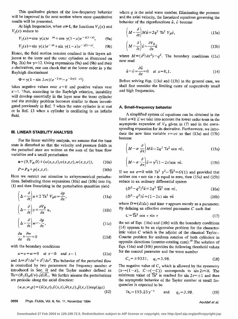
After our first experimental observation of this instability made on a small moditied Taylor-Couette cell, we de- signed a special cylindrical cell in order to obtain precise experimental results. This cell is made of an inner black anodized aluminum cylinder having a radius R 1 = 6.92 cm linked with an outer Plexiglas cylinder of radius R2= 7.70 cm, machined with a 0.01 cm tolerance, which gives a gap width d =0.775 cm and a ratio dlR t = 0.11. The radius ratio is q=(R1 lR2)=0.90 and the aspect ratio is r=hld=37.42 where the length of the cylinders is h =29 cm. A scheme of the apparatus is depicted in Fig. 3.

The experimental cell is driven by a brushless Yaskawa AC Servomotor [Fig. 3(b)] in association with a Servopack controller. With this servo drive arrangement, the angular velocity of the motor isdirectly proportional to an AC refer- ence signal given by a function generator. The two experimental parameters, frequency o and amplitude fi, are then easily regulated.

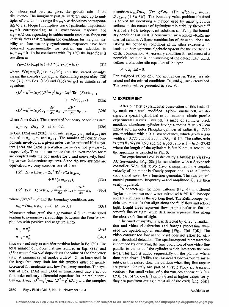
To characterize the flow patterns (Fig. 4) at different Taylor numbers we used water mixed with 2% Kalliroscope and 1% stabilizer as the working fluid. The Kalliroscope par- ticles are materials that align along the fluid flow and reflect light. Bright areas represent flow perpendicular to the observer’s line of sight, while dark areas represent flow along the observer’s line of sight.

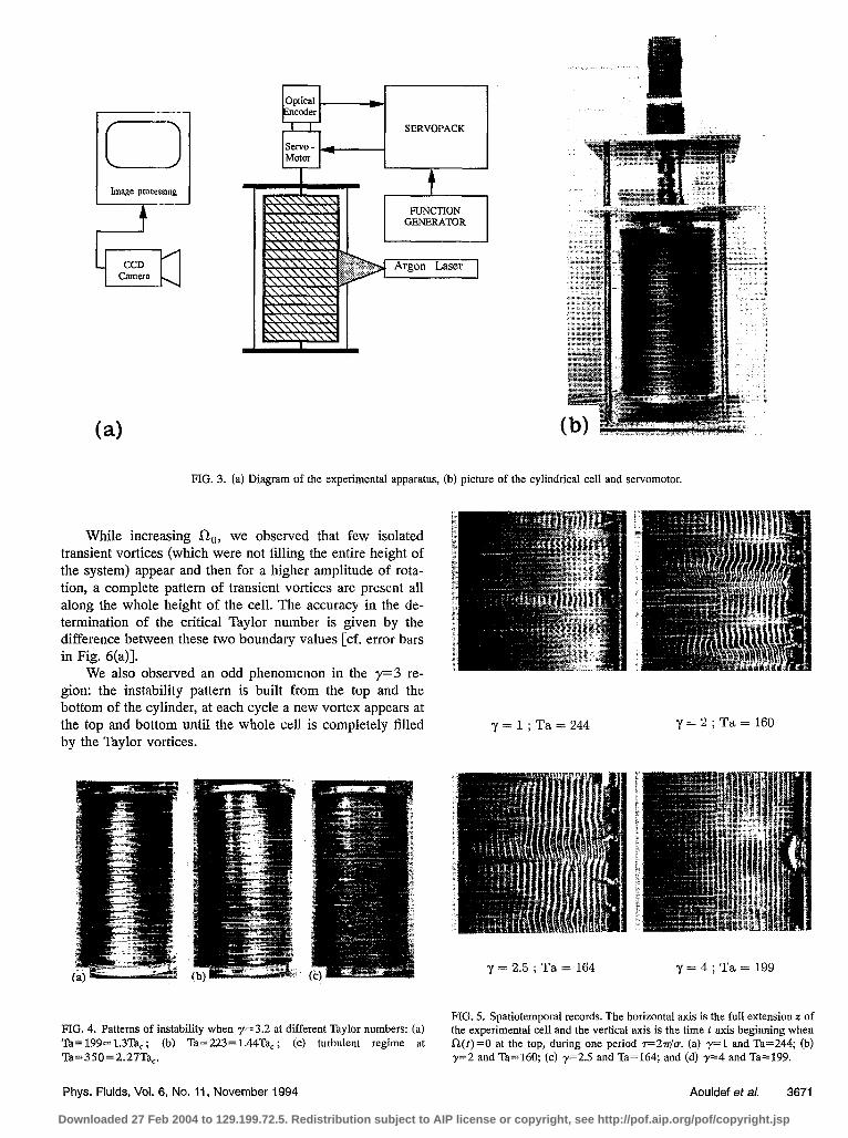
The onset of instability was detected by direct visualization and video visualization and images processing were used for spatiotemporal recording [Figs. 5(a)-5(d)]. The video contrast too low at the onset does not allow for effi- cient threshold detection. The spatiotemporal representation is obtained by observing the time evolution of one video line parallel to the axis of the cylinder which intersects the vortices. This line is added sequentially on the picture, where time runs down. Unlike the classical Taylor-Couette instability, in this pulsed flow, the vortices when they first appear are present for only one part of a cycle (they are transient vortices). For small values of y the vortices appear only in a small part of the cycle [Fig. 5(a)] and at higher values for ‘y, they are persistent during almost all of the cycle [Fig. 5(d)].

Aouidef et al.


(a)

servo - Motor

GENERATOR

FIG. 3. (a) Diagram of the experimental apparatus, (b) picture of the cylindrical cell and servomotor.

While increasing no, we observed that few isolated transient vortices (which were not filling the entire height of the system) appear and then for a higher amplitude of rotation, a complete pattern of transient vortices are present all along the whole height of the cell. The accuracy in the determination of the critical Taylor number is given by the difference between these two boundary values [cf. error bars in Fig. 6(a)].

We also observed an odd phenomenon in the y=3 region: the instability pattern is built from the top and the bottom of the cylinder, at each cycle a new vortex appears at the top and bottom until the whole cell is completely tilled by the Taylor vortices.

PIG. 4. Patterns of instability when y= 3.2 at different Taylor numbers: (a) Ta= 199= 1.3Tac ; (b) Ta=223=1.44TaC ; (cj turbulent regime at Ta=3SO=2.27Tac.


y=l;Ta=244 y=2;Ta=160

y = 2.5 ; Ta = 164 y=4;Ta=199

FIG. 5. Spatiotemporal records. The horizontal axis is the full extension I of the experimental cell and the vertical axis is the time f axis beginning when Q(t)=0 at the top, during one period r=27r/u. (a) y=l and Ta=244; (b) y=2 and Ta=160; (c) y=2.5 and Ta=164; and (d) r-4 and Ta=199.

Aouidef et a/. 3671


IflOO- p

0 (a) d a l ; ; Ib 1’2

10000-

Equation (22)

8.H

2 Equation (28)

10 1 I I T O,l 1 10 100

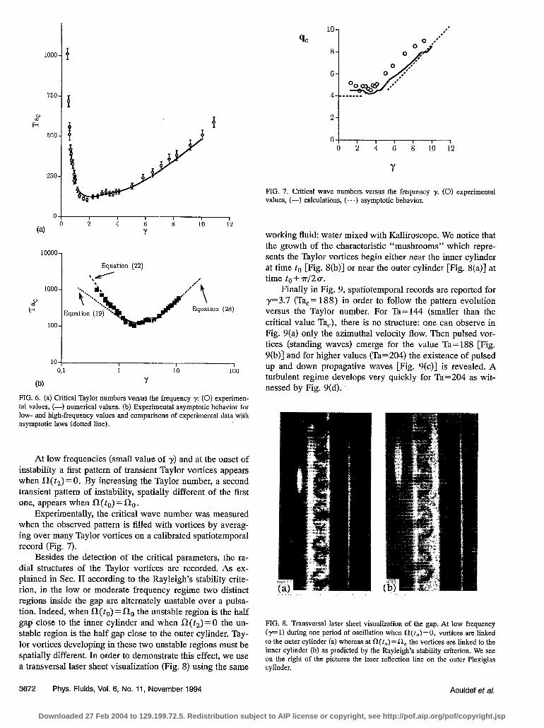
FIG. 6. (a) Critical Taylor numbers versus the frequency y (0) experimental values, (-) numerical values. (b) Experimental asymptotic behavior for low- and high-frequency values and comparisons of experimental data with asymptotic laws (dotted line).

At low frequencies (small value of r) and at the onset of instability a first pattern of transient Taylor vortices appears when n(t,) = 0. By increasing the Taylor number, a second transient pattern of instability, spatially different of the first one, appears when fi(t,) =Cn, .

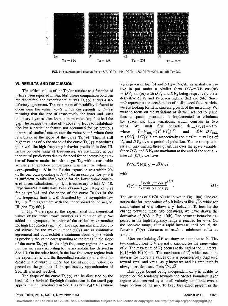
Experimentally, the critical wave number was measured when the observed pattern is filled with vortices by averag- ing over many Taylor vortices on a calibrated spatiotemporal record (Fig. 7).

Besides the detection of the critical parameters, the radial structures of the Taylor vortices are recorded. As ex- plained in Sec. II according to the Rayleigh’s stability criterion, in the low or moderate frequency regime two distinct regions inside the gap are alternately unstable over a pulsation. Indeed, when CJ(to)=fio the unstable region is the half gap close to the inner cylinder and when n(t,) = 0 the unstable region is the half gap close to the outer cylinder. Tay- lor vortices developing in these two unstable regions must be spatially different. In order to demonstrate this effect, we use a transversal laser sheet visualization (Fig. 8) using the same

0 2 4 6 8 10

Y

FIG. 7. Critical wave numbers versus the frequency 7. values, (-) calcuIations, (-. .) asymptotic behavior.

(0) experimental

working fluid: water mixed with Kalliroscope. We notice that the growth of the characteristic “mushrooms” which represents the Taylor vortices begin either near the inner cylinder at time t,, [Fig. 8(b)] or near the outer cylinder [Fig. 8(a)] at time to + rr//Za.

Finally in Fig. 9, spatiotemporal records are reported for ~3.7 (Ta,= 188) in order to follow the pattern evolution versus the Taylor number. For Ta=144 (smaller than the critical value Taa,>, there is no structure: one can observe in Fig. 9(a) only the azimuthal velocity flow. Then pulsed vortices (standing waves) emerge for the value Ta=188 [Fig. 9(b)] and for higher values (Ta=204) the existence of pulsed up and down propagative waves [Fig. 9(c)] is revealed. A turbulent regime develops very quickly for Ta=204 as wit- nessed by Fig. 9(d).

FIG. 8. Transversal laser sheet visualization of the gap. At low frequency (y 1) during one period of oscillation when n( t,,) = 0, vortices are linked to the outer cylinder (a) whereas at n(t,) =& the vortices are linked to the inner cylinder (b) as predicted by the Rayleigh’s stability criterion. We see on the right of the pictures the laser reflection line on the outer Plexiglas cylinder.



(4 (4 (d) Ta = 144 Ta = 188 Ta = 204 Ta = 282

FIG. 9. Spatiotemporal records for ~3.7. (a) Ta=144; (b) Ta= 188; (c) Ta=204; and (d) Ta=282.

VI. RESULTS AND DISCUSSION

The critical values of the Taylor number as a function of y have been reported in Fig. 6(a) where comparison between the theoretical and experimental curves Ta,( y) shows a satisfactory agreement. The maximum of instability is found to occur near the value yn= 2 which corresponds to d= 28 meaning that the size of respectively the inner and outer boundary layer reaches its maximum value (equal to half the gap). Increasing the value of y above y. leads to restabilization but a particular feature not accounted for by previous theoretical studies8 occurs near the value y1 = 3 where there is a break in the slope of the curve Ta,( y). Then at still higher values of y the shape of the curve Ta,( y) reproduces quite well the high-frequency behavior predicted in Sec. III. In the opposite range of frequencies, we are limited in our theoretical predictions due to the need for an increasing number of Fourier modes in order to get Ta, with a reasonable accuracy. In practice convergence was assumed when Ta, corresponding to N in the Fourier expansion was within 2% of the one corresponding to N+ 1. As an example, for y=3 it is sufficient to take N=3 while for the lower value considered in our calculations, y=l, it is necessary to take N=lO. Experimental results have been obtained for values of y as far as y=O.41 and the shape of the curve Ta,( y) in the low-frequency limit is well described by the asymptotic law Ta,- y-’ in agreement with the upper bound found in Sec. III [see Fig. 6(b)].

In Fig. 7 are reported the experimental and theoretical values of the critical wave number as a function of y. We added the asymptotic behavior of the critical wave number for high frequencies (qC- y). The experimental and theoretical curves for the wave number yC( y) are in qualitative agreement and both exhibit a minimum about y1=3 which is precisely the value corresponding to the break in the slope of the curve Ta,( y). In the high-frequency regime the wave number increases according to the asymptotic law derived in Sec. III. On the other hand, in the low-frequency regime both the experimental and the theoretical results show a slow increase in the wave number and the asymptotic value expected on the grounds of the quasisteady approximation of Sec. III was not reached.

The shape of the curve TaC( y) can be discussed on the basis of the inviscid Rayleigh discriminant in the small-gap approximation, introduced in Sec. II as @ = Vs(D V,) where


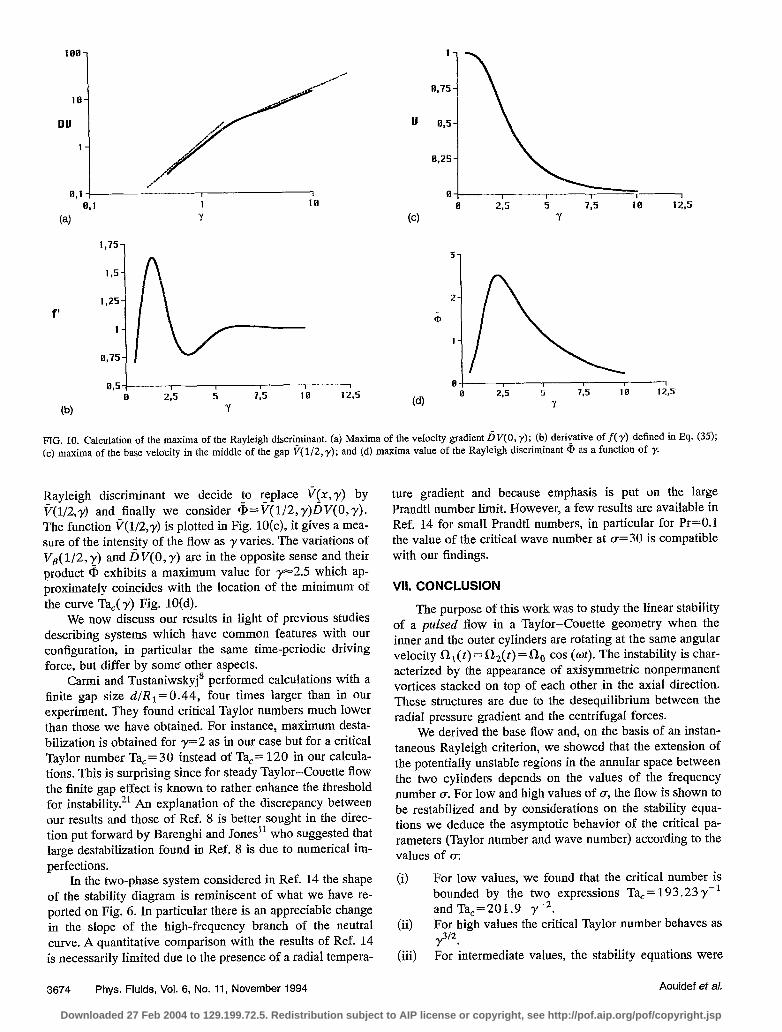
V, is given in Eq. (5) and D V, =dV,ldx its spatial derivative is put under a similar form DVB = DV1 cos (o-t) f D V, sin (at) with D VI and D V, being respectively the x derivative of VI and V, given in,Eqs. (6a) and (6b). Since --a represents the acceleration of a displaced fluid particle, we are looking for its maximum growth of the instability. We want to focus on the variations of @ with respect to y and thus a special procedure is implemented to eliminate the space and time variations, which consists in two steps. We shall first consider (Qmaxt(x, y) = l%V where v= vm,, = (VT + v$ *‘2 and = (DV;+DV;)‘i2f

bV=DV,,, are respectively the maximum values 0;

V, and DV, over a period of pulsation. The next step consists in maximizing these quantities over the space variable. Since D VI and D V2 are maximum at the end of the spatial x interval [O,l], we have

r)vaw(o, y)= Jzf( y)

with

cash y-cos y ‘I2 f(r)=r cash y+cos y * (3.5)

The variations of fiV(O, y) are shown in Fig. 10(a). One can notice that for large values of y it behaves like 3 y while for small values of y it follows a yz behavior. To localize the change between these two behaviors, we have drawn the derivative off(y) in Fig. 10(b). The constant behavior expected in the high-frequency range is reached for y=8. On the opposite range, after a rapid increase until ~1.5; the function f’(y) decreases to reach a minimum value at y3.5.

After maximizing fiV we draw an attention to ?. The two contributions to v are not maximum for the same value of X. The maximum of VT occurs at the end of the x interval [OJ] with V:(O) = 1. The maximum of Vg which occurs at midgap for moderate values of y is progressively displaced toward x= 0 and x= 1, as y increases and its amplitude is always less than one. Thus v< 6.

This upper bound being independent of y is unable to reproduce the tendency towards the Stokes boundary layer regime characterized by a small velocity amplitude over a large portion of the gap. To keep this effect present in the

Aouidef et al. 3673


(4

1,751

1,5-

1,25-

f’ l-

0,75-

a,55 a 285 5 73 10 123

(b) Y

0,75-

2-

i

l-

e’ (d) A 2:s k y 7s 16

1 12,s

FIG. 10. Calculation of the maxima of the Rayleigh discriminant. (a) Maxima of the velocity gradient L)V(O, y); (b) derivative off(y) defined in Eq. (35); (c) maxima of the base velocity in the middle of the gap v( l/2, y); and (d) maxima value of the Rayleigh discriminant @ as a function of y.

Rayleigh discriminant we decide ~0 replace v[x, 7) by v(l/2,7) and finally we consider Cp = V( l/2, y)D V( 0, y) . The function ?(1/2,y) is plotted in Fig. 10(c). it gives a mea- sure of the intensity of the flow as y varies. The variations of VB( l/2, r) and fiV(O, 7) are in the opposite sense and their product 6 exhibits a maximum value for ~2.5 which ap- proximately coincides with the location of the minimum of the curve Ta,( 7) Fig. 10(d).

ture gradient and because emphasis is put on the large Prandtl number limit. However, a few results are available in Ref. 14 for small Prandtl numbers, in particular for Pr=O.l the value of the critical wave number at a=30 is compatible with our findings.

VII. CONCLUSION

We now discuss our results in light of previous studies describing systems which have common features with our configuration, in particular the same time-periodic driving force, but differ by some-other aspects.

Carmi and Tustaniwskyj’ performed calculations with a finite gap size d/R r = 0.44, four times larger than in our experiment. They found critical Taylor numbers much lower than those we have obtained. For instance, maximum destabilization is obtained for y=2 as in our case but for a critical Taylor number Ta,= 30 instead of Ta,= 120 in our calculations. This is surprising since for steady Taylor-Couette flow

the finite gap effect is known to rather enhance the threshold for instability.“l An explanation of the discrepancy between our results and those of Ref. S is better sought in the direction put forward by Barenghi and Jones” who suggested that large destabilization found in Ref. 8 is due to numerical imperfections.

The purpose of this work was to study the linear stability of a pulsed flow in a Taylor-Couette geometry when the inner and the outer cylinders are rotating at the same angular velocity f&(t) =!&(t) = &, cos (of). The instability is characterized by the appearance of axisymmetric nonpermanent vortices stacked on top of each other in the axial direction. These structures are due to the desequilibrium between the radial pressure gradient and the centrifuga1 forces.

We derived the base flow and, on the basis of an instantaneous Rayleigh criterion, we showed that the extension of the potentially unstable regions in the annular space between the two cylinders depends on the values of the frequency number (7: For low and high values of c~, the fiow is shown to be restabilized and by considerations on the stability equations we deduce the asymptotic behavior of the critical parameters (Taylor number and wave number) according to the values of (T:

In the two-phase system considered in Ref. 14 the shape ii) For low values, we found that the critical number is of the stability diagram is reminiscent of what we have re- bounded by the two expressions Ta,=193.23y-’ ported on Fig. 6. In particular there is an appreciable change andTa,=201.9 y ‘. in the slope of the high-frequency branch of the neutral (ii) For high values the critical Taylor number behaves as curve. A quantitative comparison with the results of Ref. 14 y? is necessarily limited due to the presence of a radial tempera- {iii) For intermediate values, the stability equations were



solved on the basis of the Floquet theory leading to the marginal stability curves Ta,( r) and qc( y) presented in Sec. VI.

Furthermore, this paper describes the first experimental observation of the onset of this pulsed instability. The values of Ta, for the onset of instability were in good agreement with the theoretical results describing synchronous responses.

Work is in progress with the aim of studying and char- acterizing the “pulsed propagative vortices” showed in Fig. 9(c).

ACKNOWLEDGMENTS

During one part of this research, the first author (AA) was supported by a Doctoral Research Fellowship from the O.N.E.R.A. (Office National d’Etudes et de Recherches Aerospatiales). We acknowledge support from the G.D.R.- C.N.R.S. “Ordre et chaos dans la mat&e.” We benefited from fruitful discussions with G. M. Homsy and P. J. Mi- chard and we would like to acknowledge I. Daumont, M. Allouche, D. Vallet, and 0. Brouard for their contribution to the experimental investigation.

APPENDIX: ENERGY THEORY

We first define an inner product between two quantities f(x,z,t) and g(x,.t,t) such that

(f,g)= I,ldxl,?dqdz fg. (Al)

Then starting with the system of Eqs. (lla)-(llc) we change the scaling on u by the transformation Ta u-+u and form the inner product between the resulting equations and the velocity vector (u, u, w). After some calculations one can derive the energy identity

where

E=(u’+u”fw’), (A.34

D=(lvul”+pul”+jvwl”), (Mb)

I=2(uuVB)-(uuDVB). 63~)

Using Schwartz inequality Da t2E where c2 is a positive number we have that

1 dE I zx<-l+TaD

which implies that E--+0 as t--+m if

1 I 525.

Let

1 I G =maxr maxz

i 1 5

644)

where maxt means the maximum over the space of functions (u, u, w) which satisfy the boundary conditions (lle) and the incompressibility condition (1Od) and maxz means the maximum over a period. The stability criterion (A5) is satis- fied provided that

1 1 --a----. Ta TaE

To the variational problem

1 I

Ta,=maxl 5 ( i is associated the set of Euler-Lagrange equations

Au+2 Ta, VBu=$,

CA71

W)

@W

Au-Ta,Tu=O, Wb)

A,=$ (A9cj

which contain the time t only as a parameter. A simplifying feature arises in solving

1 1

i 1 - g=max2 Tat WO)

due to the particular form of V, given in (7). As a conse- quence the quantity I defined in (A3c) takes the form

I=11 cos t+z, sin t. (All)

Following von Kerczek and Davisz2 who got a similar expression when dealing with the stability of plane Stokes layers, we then have

z=qlf+I;)1’2, (AlZa)

I<& max [max1(Z1),maxl(12)]. (A12b)

Hence, the maximum problem (A6) reduces to two special cases:

&=fi maxi(g), &=@max,($).

One can check that the above maximum problems are equivalent respectively to the set of Eqs. (20a) and (20b) and (23a) and (23b).

‘S. H. Davis, “The stability of time-periodic flows,” Annu. Rev. Fluid Mech. 8, 57 (1976). - -

‘G. M. Homsy, “Global stability of time-dependent flows. Part 2. Modu- lated fluid layers,” J. Fluid Mech. 62, 387 (1974).

3G. Ahlers, P. C. Hohenberg, and M. Liicke, ?%ermal convection under external modulation of the driiing force J.I. Experiments,” Phys. Rev. A 32, 3493 (1985).

4R. F. Donnelly, “Experiments on the stability of viscous flow between rotating cylinders. III Enhancement of stability by modulation,” Proc. R. Sot. London Ser. A 281, 130 (1964).

‘G. Ahlers, “Effect of time-periodic modulation of the driving on the Taylor-Vortex flow,” Bull. Am. Phys. Sot. 32, 2068 (1987).

Phys. Fluids, Vol. 6, No. 11, November 1994 Aouidef et al. 3675


6P. Hall, “The stability of unsteady cylinder flows,” J. Fluid Mech. 67, 29 16A. Stegner 3 Rapport de stage de D.E.A. de Physique thiorique, Universite (1975). de Paris VI, 1993.

‘l? J. Riley and R. L. Laurence, “Linear stability of modulated circuIar Couette flow,” J. Fluid Mech. 75, 625 (1976).

*S. Carmi and J. I. Tnstaniwskyj, “Stability of modulated finite-gap cylindrical Couette flow: linear theory,” J. Fluid Mech. 108, 19 (1981).

9T. J. Walsh, W. T. Wagner, and R. J. Donnelly, “Stability of modulated Couette flow,” Phys. Rev. Lett. 58, 2543 (1988).

IoH. Kuhlmann, D. Roth, and M. Liicke, “Taylor vortex flow under har- monic modulation of the driving force,” Phys. Rev. A 39, 745 (1989).

“C E Barenghi and C. A. Jones, “Modulated Taylor-Couette flow,” J. Fluid Mech. 208, 127 (1989).

t*K. J. M&y and W. Goldburg, “Measurements on transition to turbulence in a Taylor-Couette cell with oscillatory inner cylinder,” Phys. Fluids A 5, 1438 (1993).

r3G Seminara and P. Hall, “CentrifugaI instability of a Stokes layer: linear theory,” Proc. R. Sot. London Ser. A 350, 299 (1976).

14R. J. Braun, G. B. McFadden, B. T. Murray, S. R. Coriell, M. E. Glicks- man, and M. E. Selleck, “Asymptotic behavior of modulated Taylor- Couette flow with a crystalline inner cylinder,” Phys. Fluids A 5, 1891 (1993).

*‘B. T. Murray, G. B. McFadden, and S. R. Coriell, “Stabilization of Taylor-Couette flow due to time-periodic outer cylinder rotation,” Phys. Fluids A 2, 2147 (1990).

“I. Mutabazi, C. Normand, and J. E. Wesfreid, “Gap size effects on cen- trifugally and rotationally driven instabilities,” Phys. Fluids A 4, 1199 (1992).

“I. Mutabazi and J. E. Wesfreid, “Coriolis force and centrifugal force induced flow instabilities,” in Instabilities and Nonequilibrium Structures N, edited by E. Tirapegui and W. Zeller (Kluwer Academic, Dordrecht, 1993), pp. 301-316.

t9S. Chandrasekhar, Hydrodynamic and Hydromagnetic Stability (Oxford University Press, London, 1961).

2oP. G. Drazin and W. H. Reid, Hydrodynamic Stability (Cambridge Univer- sity Press, Cambridge, 1981).

*rE. R. Krueger, A. Gross, and R. C. Di Prima, “On the relative importance of Taylor-vortex and non-axisymmetric modes in flow between rotating cylinders,” J. Fluid Mech. 24, 521 (1966).

%. von Kerczek and S. H. Davis, “The stability of oscillatory Stokes layers,” Stud. App. Math. LI, 239 (1972).

=L. Cesari, Asymptotic Behavior and Stability Problems in Ordinary Dif- ferentiar Equations (Springer-Verlag, Berlin, 1963).

aA. Aouidef, “Instabilitb hydrodynamiques dues aux effets des forces cen- trifuges et de rotation,” these de doctorat de I’Universitd Paris VI, 1994.

3676 Phys. Fluids, Vol. 6, No. 11, November 1994 Aouidef ef al.


Centrifugal instability of pulsed...

Documents

Transcript of Centrifugal instability of pulsed...