Basic tutorial to CPMD calculations - Unistra and Parinnello Molecular Dynamics Basic tutorial to...

Car and Parinnello Molecular Dynamicshttp://www.cpmd.org/

Basic tutorial to CPMD calculations

Sébastien LE ROUX [email protected]

INSTITUT DE PHYSIQUE ET DE CHIMIE DES MATÉRIAUX DE STRASBOURG,DÉPARTEMENT DES MATÉRIAUX ORGANIQUES,

23 RUE DU LOESS, BP43,F-67034 STRASBOURG CEDEX 2, FRANCE

MARCH 23, 2016

http://www.cpmd.org/

mailo:[email protected]

Contents

Contents ii

List of figures iii

List of tables v

1 CPMD basics 1

1.1 General ideas on the CPMD method . . . . . . . . . . . . . . . . . . . . . . . . . . . . 11.2 Structure of the CPMD input file . . . . . . . . . . . . . . . . . . . . . . . . . . . . . . 2

1.2.1 The INFO section . . . . . . . . . . . . . . . . . . . . . . . . . . . . . . . . . . 21.2.2 The CPMD section . . . . . . . . . . . . . . . . . . . . . . . . . . . . . . . . . . 31.2.3 The DFT section . . . . . . . . . . . . . . . . . . . . . . . . . . . . . . . . . . . 41.2.4 The VDW section . . . . . . . . . . . . . . . . . . . . . . . . . . . . . . . . . . . 41.2.5 The PROP section . . . . . . . . . . . . . . . . . . . . . . . . . . . . . . . . . . 51.2.6 The SYSTEM section . . . . . . . . . . . . . . . . . . . . . . . . . . . . . . . . . 61.2.7 The ATOMS section . . . . . . . . . . . . . . . . . . . . . . . . . . . . . . . . . 7

2 CPMD calculations 9

2.1 Wavefunction optimization . . . . . . . . . . . . . . . . . . . . . . . . . . . . . . . . . 92.2 Geometry optimization . . . . . . . . . . . . . . . . . . . . . . . . . . . . . . . . . . . 10

2.2.1 Using the OPTIMIZE GEOMETRY keywords = the automatic way . . . . . . . . . 102.2.2 Using Molecular Dynamics + Friction forces = the manual way . . . . . . . . . 11

2.3 Free CPMD dynamics . . . . . . . . . . . . . . . . . . . . . . . . . . . . . . . . . . . . 122.4 Temperature control CPMD dynamics . . . . . . . . . . . . . . . . . . . . . . . . . . . 132.5 Nosé thermostat . . . . . . . . . . . . . . . . . . . . . . . . . . . . . . . . . . . . . . . 142.6 Electronic density of states . . . . . . . . . . . . . . . . . . . . . . . . . . . . . . . . . 14

2.6.1 Kohn-Sham energies calculation . . . . . . . . . . . . . . . . . . . . . . . . . . 142.6.2 Free energy calculation . . . . . . . . . . . . . . . . . . . . . . . . . . . . . . . 15

2.7 3D visualization of orbitals, electronic densities . . . . . . . . . . . . . . . . . . . . . . 162.7.1 CPMD keywords . . . . . . . . . . . . . . . . . . . . . . . . . . . . . . . . . . 162.7.2 CPMD2CUBE . . . . . . . . . . . . . . . . . . . . . . . . . . . . . . . . . . . 16

2.8 Electron localization function ELF . . . . . . . . . . . . . . . . . . . . . . . . . . . . . 172.8.1 CPMD keywords . . . . . . . . . . . . . . . . . . . . . . . . . . . . . . . . . . 172.8.2 CPMD2CUBE . . . . . . . . . . . . . . . . . . . . . . . . . . . . . . . . . . . 17

2.9 Maximally localized Wannier functions . . . . . . . . . . . . . . . . . . . . . . . . . . 182.9.1 CPMD keywords . . . . . . . . . . . . . . . . . . . . . . . . . . . . . . . . . . 18

i

2.9.2 CPMD2CUBE . . . . . . . . . . . . . . . . . . . . . . . . . . . . . . . . . . . 182.10 Restarts . . . . . . . . . . . . . . . . . . . . . . . . . . . . . . . . . . . . . . . . . . . 19

3 Controlling adiabaticity in CPMD 21

3.1 Car-Parrinello equations of motion . . . . . . . . . . . . . . . . . . . . . . . . . . . . . 213.2 How to control adiabaticity ? . . . . . . . . . . . . . . . . . . . . . . . . . . . . . . . . 22

4 Parameters of the Nosé thermostat 25

4.1 Nosé thermostats in the CPMD method . . . . . . . . . . . . . . . . . . . . . . . . . . 254.2 Choosing the parameters . . . . . . . . . . . . . . . . . . . . . . . . . . . . . . . . . . 26

4.2.1 Ekin,e . . . . . . . . . . . . . . . . . . . . . . . . . . . . . . . . . . . . . . . . 264.2.2 QR and Qe . . . . . . . . . . . . . . . . . . . . . . . . . . . . . . . . . . . . . 26

ii

List of Figures

3.1 Schematic representation of the vibration frequencies of the ionic and the electronic sub-system in

CPMD. Electronic frequencies have to be higher than the ionic frequencies, and the two must not

overlap. . . . . . . . . . . . . . . . . . . . . . . . . . . . . . . . . . . . . . . . . . . . . . . . . 223.2 Schematic representation of the evolution of EKINC, EKS, ECLASSIC and EHAM during a

CPMD calculation. The effect of the modification of µ and/or ∆tmax is shown on the evolution

of ECLASSIC and EKINC. . . . . . . . . . . . . . . . . . . . . . . . . . . . . . . . . . . . . . . 24

4.1 Schematic representation of the thermal frequencies of the ionic and the electronic sub-system,

as well as the Nosé thermostats for both sub-systems in CPMD. Electronic frequencies (fictitious

electrons + thermostat) have to be higher than the ionic frequencies (ions + thermostat), and the

two sets of frequencies must not overlap. . . . . . . . . . . . . . . . . . . . . . . . . . . . . . . . 27

iii

List of Tables

2.1 Typical output of a geometry optimization run in the CPMD code. . . . . . . . . . . . . . . . . . 112.2 Typical output of a Car-Parrinello molecular dynamics run in the CPMD code. . . . . . . . . . . 12

v

CPMD basics

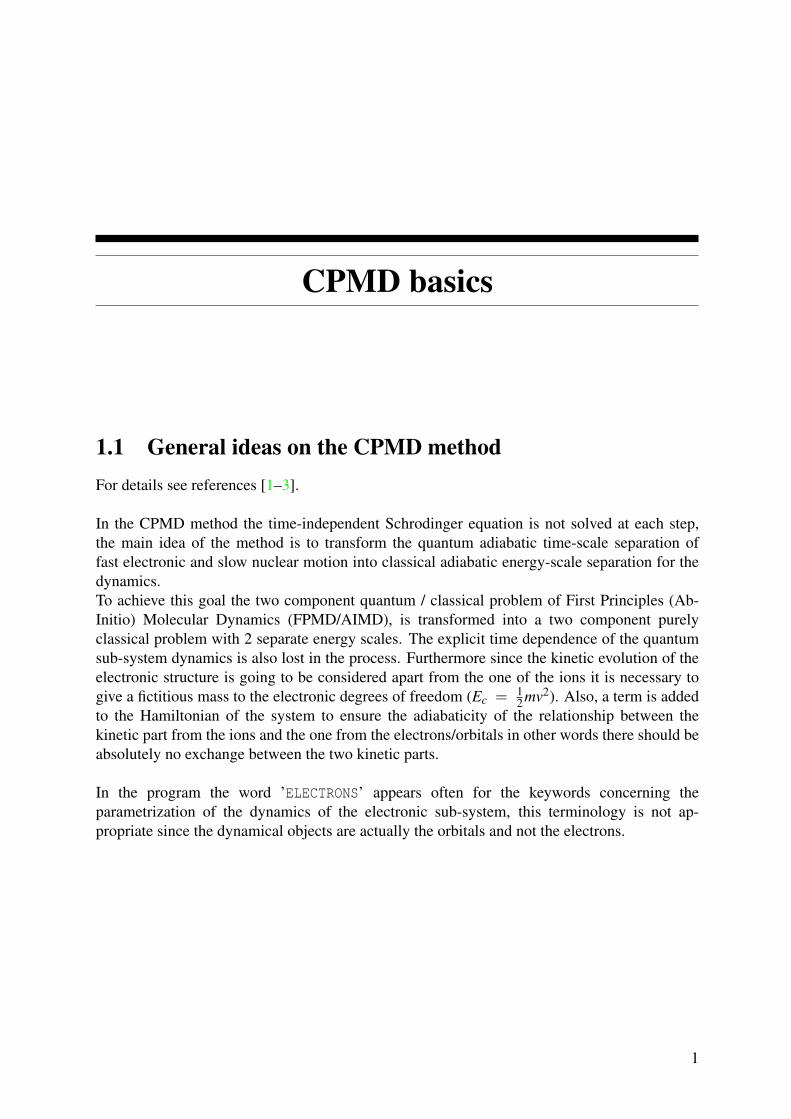
1.1 General ideas on the CPMD method

For details see references [1–3].

In the CPMD method the time-independent Schrodinger equation is not solved at each step,the main idea of the method is to transform the quantum adiabatic time-scale separation offast electronic and slow nuclear motion into classical adiabatic energy-scale separation for thedynamics.To achieve this goal the two component quantum / classical problem of First Principles (Ab-Initio) Molecular Dynamics (FPMD/AIMD), is transformed into a two component purelyclassical problem with 2 separate energy scales. The explicit time dependence of the quantumsub-system dynamics is also lost in the process. Furthermore since the kinetic evolution of theelectronic structure is going to be considered apart from the one of the ions it is necessary togive a fictitious mass to the electronic degrees of freedom (Ec = 1

2mv2). Also, a term is addedto the Hamiltonian of the system to ensure the adiabaticity of the relationship between thekinetic part from the ions and the one from the electrons/orbitals in other words there should beabsolutely no exchange between the two kinetic parts.

In the program the word ’ELECTRONS’ appears often for the keywords concerning theparametrization of the dynamics of the electronic sub-system, this terminology is not ap-propriate since the dynamical objects are actually the orbitals and not the electrons.

1

Chapter 1. CPMD basics 2

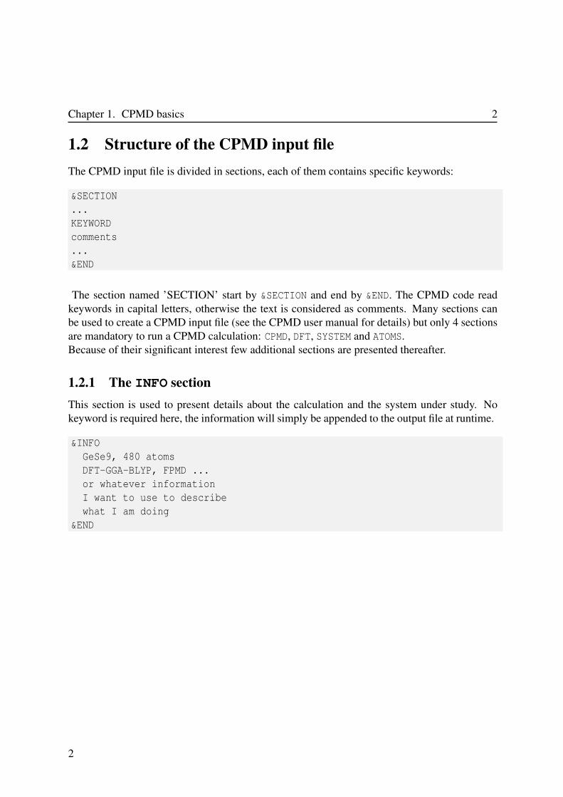
1.2 Structure of the CPMD input file

The CPMD input file is divided in sections, each of them contains specific keywords:

&SECTION

...

KEYWORD

comments

...

&END

The section named ’SECTION’ start by &SECTION and end by &END. The CPMD code readkeywords in capital letters, otherwise the text is considered as comments. Many sections canbe used to create a CPMD input file (see the CPMD user manual for details) but only 4 sectionsare mandatory to run a CPMD calculation: CPMD, DFT, SYSTEM and ATOMS.Because of their significant interest few additional sections are presented thereafter.

1.2.1 The INFO section

This section is used to present details about the calculation and the system under study. Nokeyword is required here, the information will simply be appended to the output file at runtime.

&INFO

GeSe9, 480 atoms

DFT-GGA-BLYP, FPMD ...

or whatever information

I want to use to describe

what I am doing

&END

2

3 1.2. Structure of the CPMD input file

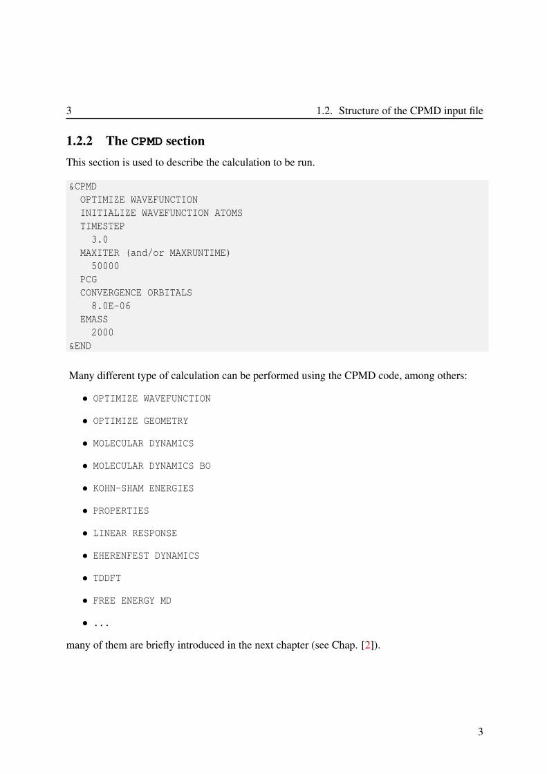
1.2.2 The CPMD section

This section is used to describe the calculation to be run.

&CPMD

OPTIMIZE WAVEFUNCTION

INITIALIZE WAVEFUNCTION ATOMS

TIMESTEP

3.0

MAXITER (and/or MAXRUNTIME)

50000

PCG

CONVERGENCE ORBITALS

8.0E-06

EMASS

2000

&END

Many different type of calculation can be performed using the CPMD code, among others:

• OPTIMIZE WAVEFUNCTION

• OPTIMIZE GEOMETRY

• MOLECULAR DYNAMICS

• MOLECULAR DYNAMICS BO

• KOHN-SHAM ENERGIES

• PROPERTIES

• LINEAR RESPONSE

• EHERENFEST DYNAMICS

• TDDFT

• FREE ENERGY MD

• ...

many of them are briefly introduced in the next chapter (see Chap. [2]).

3


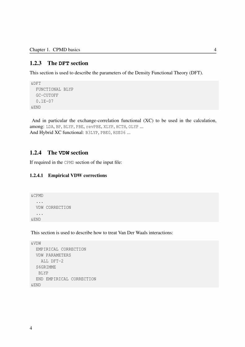
1.2.3 The DFT section

This section is used to describe the parameters of the Density Functional Theory (DFT).

&DFT

FUNCTIONAL BLYP

GC-CUTOFF

0.1E-07

&END

And in particular the exchange-correlation functional (XC) to be used in the calculation,among: LDA, BP, BLYP, PBE, revPBE, XLYP, HCTH, OLYP ...And Hybrid XC functional: B3LYP, PBE0, HSE06 ...

1.2.4 The VDW section

If required in the CPMD section of the input file:

1.2.4.1 Empirical VDW corrections

&CPMD

...

VDW CORRECTION

...

&END

This section is used to describe how to treat Van Der Waals interactions:

&VDW

EMPIRICAL CORRECTION

VDW PARAMETERS

ALL DFT-2

S6GRIMME

BLYP

END EMPIRICAL CORRECTION

&END

4


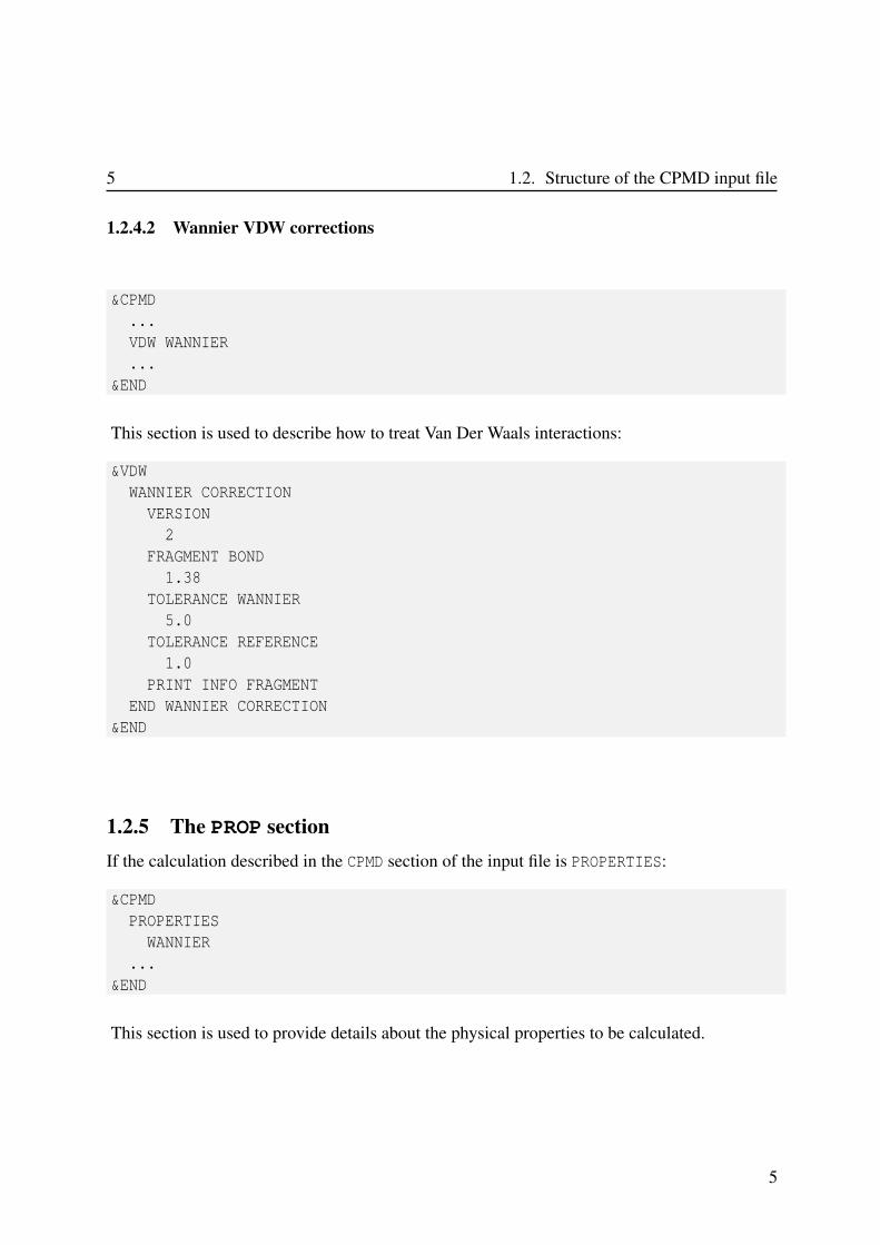
1.2.4.2 Wannier VDW corrections

&CPMD

...

VDW WANNIER

...

&END

This section is used to describe how to treat Van Der Waals interactions:

&VDW

WANNIER CORRECTION

VERSION

2

FRAGMENT BOND

1.38

TOLERANCE WANNIER

5.0

TOLERANCE REFERENCE

1.0

PRINT INFO FRAGMENT

END WANNIER CORRECTION

&END

1.2.5 The PROP section

If the calculation described in the CPMD section of the input file is PROPERTIES:

&CPMD

PROPERTIES

WANNIER

...

&END

This section is used to provide details about the physical properties to be calculated.

5


&PROP

LOCALIZE

PROJECT WAVEFUNCTION

POPULATION ANALYSIS MULLIKEN

&END

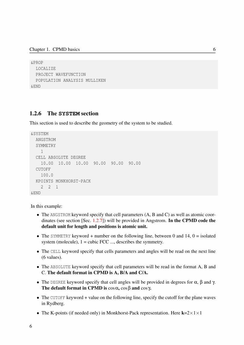
1.2.6 The SYSTEM section

This section is used to describe the geometry of the system to be studied.

&SYSTEM

ANGSTROM

SYMMETRY

1

CELL ABSOLUTE DEGREE

10.00 10.00 10.00 90.00 90.00 90.00

CUTOFF

100.0

KPOINTS MONKHORST-PACK

2 2 1

&END

In this example:

• The ANGSTROM keyword specify that cell parameters (A, B and C) as well as atomic coor-dinates (see section [Sec. 1.2.7]) will be provided in Angstrom. In the CPMD code the

default unit for length and positions is atomic unit.

• The SYMMETRY keyword + number on the following line, between 0 and 14, 0 = isolatedsystem (molecule), 1 = cubic FCC ..., describes the symmetry.

• The CELL keyword specify that cells parameters and angles will be read on the next line(6 values).

• The ABSOLUTE keyword specify that cell parameters will be read in the format A, B andC. The default format in CPMD is A, B/A and C/A.

• The DEGREE keyword specify that cell angles will be provided in degrees for α, β and γ.The default format in CPMD is cosα, cosβ and cosγ.

• The CUTOFF keyword + value on the following line, specify the cutoff for the plane wavesin Rydberg.

• The K-points (if needed only) in Monkhorst-Pack representation. Here k=2×1×1

6


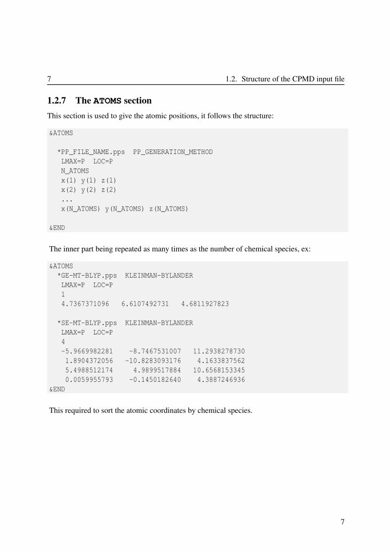
1.2.7 The ATOMS section

This section is used to give the atomic positions, it follows the structure:

&ATOMS

*PP_FILE_NAME.pps PP_GENERATION_METHOD

LMAX=P LOC=P

N_ATOMS

x(1) y(1) z(1)

x(2) y(2) z(2)

...

x(N_ATOMS) y(N_ATOMS) z(N_ATOMS)

&END

The inner part being repeated as many times as the number of chemical species, ex:

&ATOMS

*GE-MT-BLYP.pps KLEINMAN-BYLANDER

LMAX=P LOC=P

1

4.7367371096 6.6107492731 4.6811927823

*SE-MT-BLYP.pps KLEINMAN-BYLANDER

LMAX=P LOC=P

4

-5.9669982281 -8.7467531007 11.2938278730

1.8904372056 -10.8283093176 4.1633837562

5.4988512174 4.9899517884 10.6568153345

0.0059955793 -0.1450182640 4.3887246936

&END

This required to sort the atomic coordinates by chemical species.

7


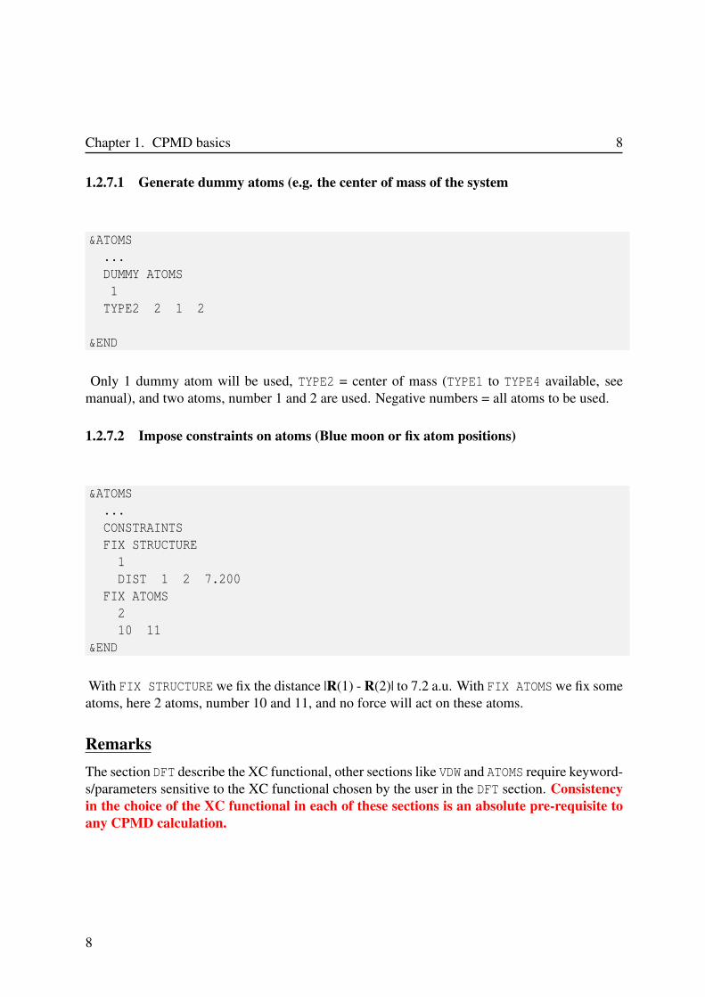
1.2.7.1 Generate dummy atoms (e.g. the center of mass of the system

&ATOMS

...

DUMMY ATOMS

1

TYPE2 2 1 2

&END

Only 1 dummy atom will be used, TYPE2 = center of mass (TYPE1 to TYPE4 available, seemanual), and two atoms, number 1 and 2 are used. Negative numbers = all atoms to be used.

1.2.7.2 Impose constraints on atoms (Blue moon or fix atom positions)

&ATOMS

...

CONSTRAINTS

FIX STRUCTURE

1

DIST 1 2 7.200

FIX ATOMS

2

10 11

&END

With FIX STRUCTURE we fix the distance |R(1) - R(2)| to 7.2 a.u. With FIX ATOMS we fix someatoms, here 2 atoms, number 10 and 11, and no force will act on these atoms.

Remarks

The section DFT describe the XC functional, other sections like VDW and ATOMS require keyword-s/parameters sensitive to the XC functional chosen by the user in the DFT section. Consistency

in the choice of the XC functional in each of these sections is an absolute pre-requisite to

any CPMD calculation.

8

CPMD calculations

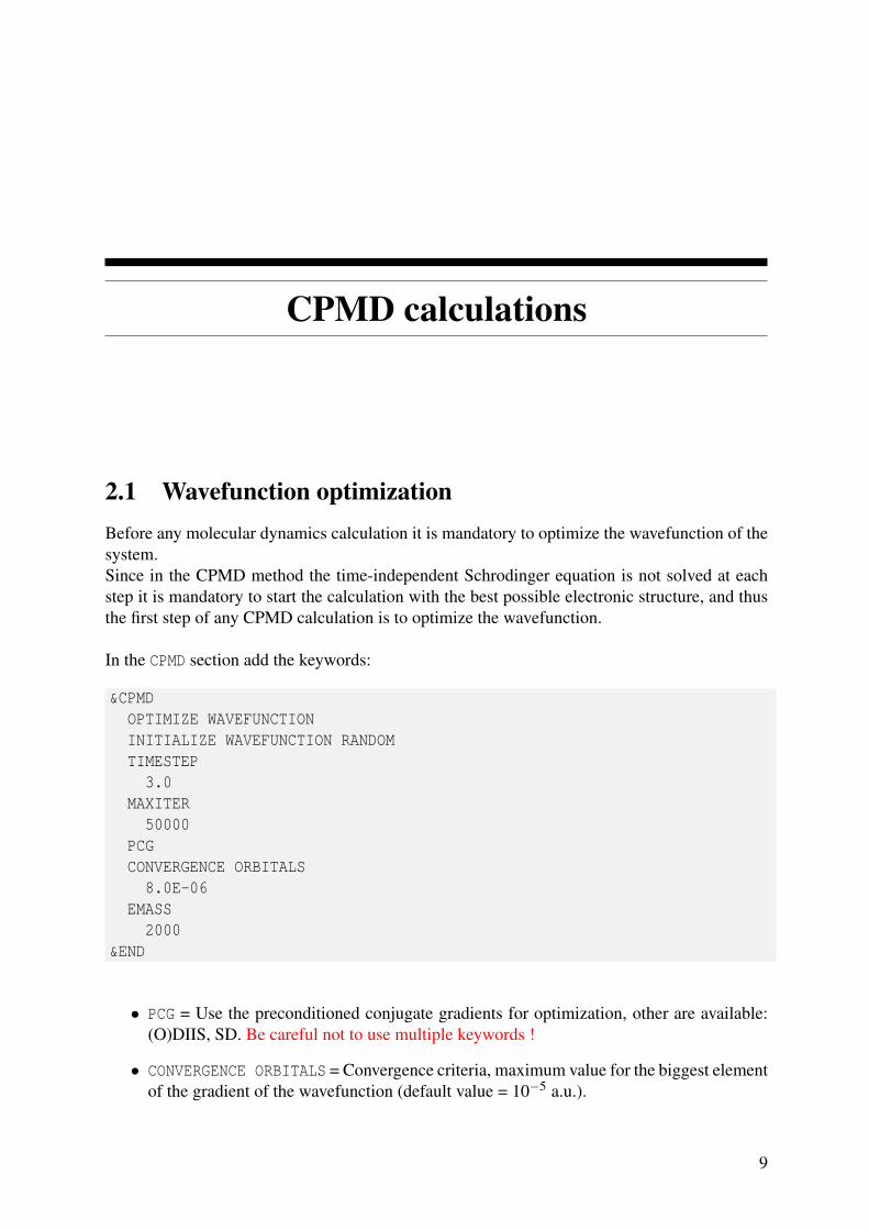
2.1 Wavefunction optimization

Before any molecular dynamics calculation it is mandatory to optimize the wavefunction of thesystem.Since in the CPMD method the time-independent Schrodinger equation is not solved at eachstep it is mandatory to start the calculation with the best possible electronic structure, and thusthe first step of any CPMD calculation is to optimize the wavefunction.

In the CPMD section add the keywords:

&CPMD

OPTIMIZE WAVEFUNCTION

INITIALIZE WAVEFUNCTION RANDOM

TIMESTEP

3.0

MAXITER

50000

PCG

CONVERGENCE ORBITALS

8.0E-06

EMASS

2000

&END

• PCG = Use the preconditioned conjugate gradients for optimization, other are available:(O)DIIS, SD. Be careful not to use multiple keywords !

• CONVERGENCE ORBITALS = Convergence criteria, maximum value for the biggest elementof the gradient of the wavefunction (default value = 10−5 a.u.).

9

Chapter 2. CPMD calculations 10

• MAXITER = Maximum number of optimization steps (Default 10000), in the case of wave-function optimization the keyword MAXSTEP, which is a parameter required for geometryoptimization or molecular dynamics, can also be used.

• WAVEFUNCTION can also be initialized from the atom positions, then instead of RANDOMuse ATOMS as keyword.

• EMASS = Fiction electron mass in a.u. (default value = 400 a.u.)

2.2 Geometry optimization

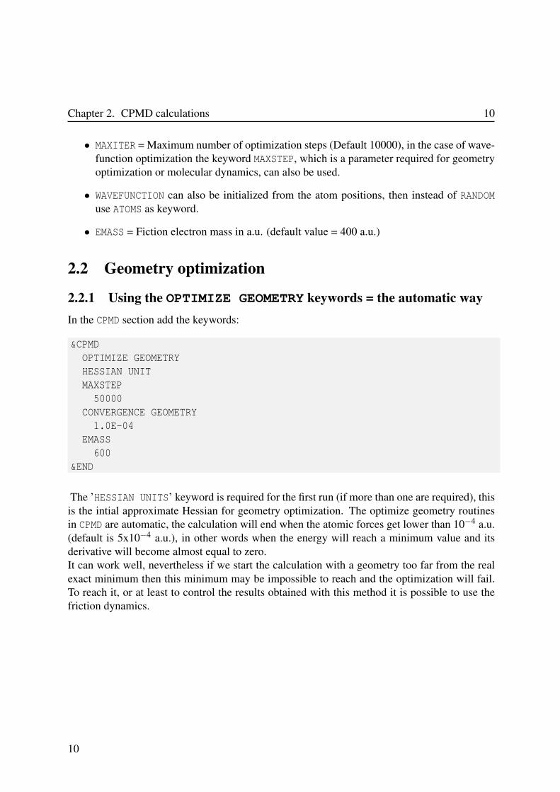
2.2.1 Using the OPTIMIZE GEOMETRY keywords = the automatic way


&CPMD

OPTIMIZE GEOMETRY

HESSIAN UNIT

MAXSTEP

50000

CONVERGENCE GEOMETRY

1.0E-04

EMASS

600

&END

The ’HESSIAN UNITS’ keyword is required for the first run (if more than one are required), thisis the intial approximate Hessian for geometry optimization. The optimize geometry routinesin CPMD are automatic, the calculation will end when the atomic forces get lower than 10−4 a.u.(default is 5x10−4 a.u.), in other words when the energy will reach a minimum value and itsderivative will become almost equal to zero.It can work well, nevertheless if we start the calculation with a geometry too far from the realexact minimum then this minimum may be impossible to reach and the optimization will fail.To reach it, or at least to control the results obtained with this method it is possible to use thefriction dynamics.

10

11 2.2. Geometry optimization

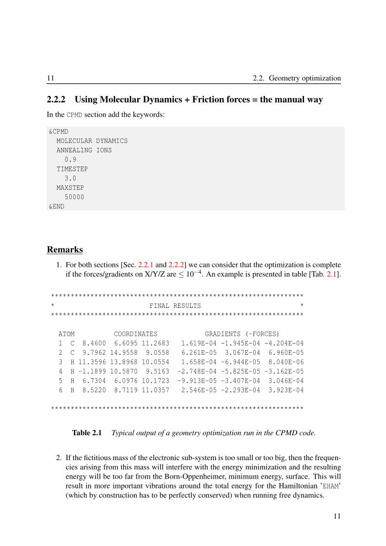
2.2.2 Using Molecular Dynamics + Friction forces = the manual way


&CPMD

MOLECULAR DYNAMICS

ANNEALING IONS

0.9

TIMESTEP

3.0

MAXSTEP

50000

&END

Remarks

1. For both sections [Sec. 2.2.1 and 2.2.2] we can consider that the optimization is completeif the forces/gradients on X/Y/Z are ≤ 10−4. An example is presented in table [Tab. 2.1].

****************************************************************

* FINAL RESULTS *

****************************************************************

ATOM COORDINATES GRADIENTS (-FORCES)

1 C 8.4600 6.6095 11.2683 1.619E-04 -1.945E-04 -4.204E-04

2 C 9.7962 14.9558 9.0558 6.261E-05 3.067E-04 6.960E-05

3 H 11.3596 13.8968 10.0554 1.658E-04 -6.944E-05 8.040E-06

4 H -1.1899 10.5870 9.5163 -2.748E-04 -5.825E-05 -3.162E-05

5 H 6.7304 6.0976 10.1723 -9.913E-05 -3.407E-04 3.046E-04

6 H 8.5220 8.7119 11.0357 2.546E-05 -2.293E-04 3.923E-04

****************************************************************

Table 2.1 Typical output of a geometry optimization run in the CPMD code.

2. If the fictitious mass of the electronic sub-system is too small or too big, then the frequen-cies arising from this mass will interfere with the energy minimization and the resultingenergy will be too far from the Born-Oppenheimer, minimum energy, surface. This willresult in more important vibrations around the total energy for the Hamiltonian ’EHAM’(which by construction has to be perfectly conserved) when running free dynamics.

11


2.3 Free CPMD dynamics


&CPMD

MOLECULAR DYNAMICS

TIMESTEP

3.0

MAXSTEP

50000

&END

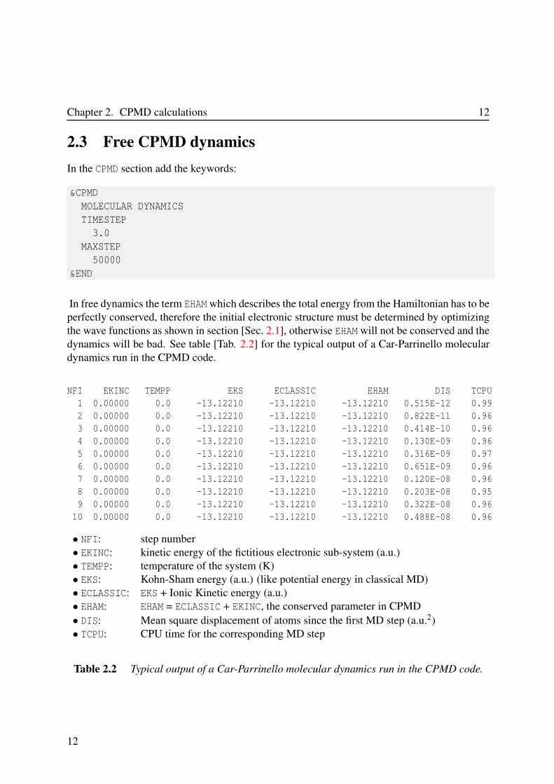
In free dynamics the term EHAM which describes the total energy from the Hamiltonian has to beperfectly conserved, therefore the initial electronic structure must be determined by optimizingthe wave functions as shown in section [Sec. 2.1], otherwise EHAM will not be conserved and thedynamics will be bad. See table [Tab. 2.2] for the typical output of a Car-Parrinello moleculardynamics run in the CPMD code.

NFI EKINC TEMPP EKS ECLASSIC EHAM DIS TCPU

1 0.00000 0.0 -13.12210 -13.12210 -13.12210 0.515E-12 0.99

2 0.00000 0.0 -13.12210 -13.12210 -13.12210 0.822E-11 0.96

3 0.00000 0.0 -13.12210 -13.12210 -13.12210 0.414E-10 0.96

4 0.00000 0.0 -13.12210 -13.12210 -13.12210 0.130E-09 0.96

5 0.00000 0.0 -13.12210 -13.12210 -13.12210 0.316E-09 0.97

6 0.00000 0.0 -13.12210 -13.12210 -13.12210 0.651E-09 0.96

7 0.00000 0.0 -13.12210 -13.12210 -13.12210 0.120E-08 0.96

8 0.00000 0.0 -13.12210 -13.12210 -13.12210 0.203E-08 0.95

9 0.00000 0.0 -13.12210 -13.12210 -13.12210 0.322E-08 0.96

10 0.00000 0.0 -13.12210 -13.12210 -13.12210 0.488E-08 0.96

• NFI: step number• EKINC: kinetic energy of the fictitious electronic sub-system (a.u.)• TEMPP: temperature of the system (K)• EKS: Kohn-Sham energy (a.u.) (like potential energy in classical MD)• ECLASSIC: EKS + Ionic Kinetic energy (a.u.)• EHAM: EHAM = ECLASSIC + EKINC, the conserved parameter in CPMD• DIS: Mean square displacement of atoms since the first MD step (a.u.2)• TCPU: CPU time for the corresponding MD step

Table 2.2 Typical output of a Car-Parrinello molecular dynamics run in the CPMD code.

12

13 2.4. Temperature control CPMD dynamics

Remarks

1. When changing the calculation from ’OPTIMIZE GEOMETRY’ to ’MOLECULAR DYNAMICS’one must not use the velocities from the restart file.

2. In the output file labelled ’ENERGIES’ the first column presents the kinetic energy of thefictitious electronic part. If the values in this column are too important and/or if they aresubject to too much variation then there is a problem in the calculation.

2.4 Temperature control CPMD dynamics


&CPMD

MOLECULAR DYNAMICS

TIMESTEP

3.0

MAXSTEP

50000

TEMPCONTROL IONS

800 100

&END

The first number is the target temperature, and the second is the tolerance around this value.Both are given in K. In this example the temperature of the system is to be oscillated around800 +/- 100 K, if the temperature goes bellow 700 K or higher than 900 K then it is readjusted.Optional keywords for the fictitious electronic sub-system are:

&CPMD

TEMPCONTROL ELECTRONS

0.04 0.01

&END

The first number is the target fictitious kinetic energy, and the second is the tolerance aroundthis value. Both are given in atomic units.

13


2.5 Nosé thermostat


&CPMD

MOLECULAR DYNAMICS

TIMESTEP

3.0

MAXSTEP

50000

NOSE IONS

1000 200

NOSE ELECTRONS

0.2 600

&END

In the first case (IONS) the first number represents the target thermodynamic temperature in K,the second the thermostat frequency in cm−1. In the second case (ELECTRONS) the first numberrepresents the target fictitious kinetic energy, the second the thermostat frequency in cm−1. Thevalue of the target fictitious kinetic energy has to be of the order of the value of the fictitiouskinetic energy observed in a free-dynamics simulation (little bit higher is good).When the Nosé thermostat is used, the frequency must be much higher for the ELECTRONS

than for the IONS. The two Nosé thermostats (IONS and ELECTRONS) must played on distinctfrequencies yet leading to a similar thermalization for the two sub-systems, see chapter [Chap.4] for details.

2.6 Electronic density of states

Note that several methods exist in order to achieve this calculation, two of these methods areintroduced hereafter.

2.6.1 Kohn-Sham energies calculation


&CPMD

...

RESTART WAVEFUNCTION COORDINATES LATEST

KOHN-SHAM ENERGIES

100

...

&END

14

15 2.6. Electronic density of states

The number that appears after the keyword KOHN-SHAM ENERGIES represents the number ofunoccupied electronic states, this number depends on the system and has to be large enoughso that the energy of the electronic states that surround the HOMO-LUMO gap are perfectlyconverged. This calculation can only be performed using a converged electronic structure, thatis why one has to use a restart file (see section [Sec. 2.10] for detail) from a wave function opti-mization (see section [Sec. 2.1] for detail). Also worth to mention is the fact that this calculationrequires significantly more memory than a standard CPMD calculation, both wavefunctions andHamiltonian required to be stored in memory, the latest being diagonalized.Van Der Walls interactions must be turned off for this calculation.

2.6.2 Free energy calculation


&CPMD

...

OPTIMIZE WAVEFUNCTIONS

FREE ENERGY FUNCTIONAL

INITIALIZE WAVEFUNCTIONS RANDOM

TROTTER FACTOR

0.001

BOGOLIUBOV CORRECTION

LANCZOS DIAGONALISATION

LANCZOS PARAMETERS n=5

1000 8 22 1.D-8

0.05 1.D-10

0.01 1.D-12

0.0025 1.D-15

0.001 1.D-17

ANDERSON MIXING=3

1. 0.1

0.01 0.1

0.005 0.1

TEMPERATURE ELECTRON

300.0

...

&END

The free functional calculation uses the Fermi-Dirac distribution in order to fill the electronicstates as a function of the temperature. The first part of the calculation is a Born-Oppenheimerwave function optimization to calculate the electronic structure of the system. The parametersprovided above likely depend on the system under study.

15


2.7 3D visualization of orbitals, electronic densities

The calculation and the extraction of the orbitals and densities is done using the CPMD code,afterwards the creation of the input files for 3D visualization is done using the CPMD2CUBEcode.

2.7.1 CPMD keywords


&CPMD

...

RHOOUT BANDS

4

-805 -806 -807 -808

...

&END

Using the RHOOUT + BANDS keywords a certain number of bands or orbitals will be plotted.The number of orbitals is given in the second line, and their index, starting from 1, is given inthe third line:

• positive index (ex: 806) = the electronic density is written, output files are stored inDENSITY.index, ex: DENSITY.806

• negative index (ex: -806) = the wavefunction is written, output files are stored inWAVEFUNCTION.index, ex: WAVEFUNCTION.806

2.7.2 CPMD2CUBE

The exact command depends on the nature of the object to be visualized:

• For a DENSITY:

./cpmd2cube.x -dens -centre DENSITY.806

• For a WAVEFUNCTION:

./cpmd2cube.x -wave -centre WAVEFUNCTION.806

It is also possible to use the -inbox keyword to force atoms to be put inside the simulation boxwhen periodic boundary conditions are used.

16

17 2.8. Electron localization function ELF

2.8 Electron localization function ELF

The formalism of the electron localization function ELF [4–7] provides a deeper insight on thebonding localization. More precisely the ELF gives information on the degree of localization ofthe electronic density. When the ELF values are close to the maximum, it is possible to identify,for a given value, centers in space, so-called attractors, which are surrounded by disjoint ELFisosurfaces, so-called basins, defining different charge localization domains. Merging of dif-ferent basins for slightly lower values of ELF may reveal the existence of localization domainshaving in common more than one attractor. This gives indications on the centers involved in thebonding and on the spatial extension of this latter. [8]The calculation of the ELF requires to add a single keyword to the CPMD section of theinput file, afterwards the creation of the input files for 3D visualization is done using theCPMD2CUBE code.

2.8.1 CPMD keywords


&CPMD

...

ELF

...

&END

At CPMD runtime this keyword will generate the creation of a file named ELF in the activedirectory.

2.8.2 CPMD2CUBE

The ELF file is a density file similar to the DENSITY files and has to be converted using theCPMD2CUBE code.

./cpmd2cube.x -dens -centre ELF

17


2.9 Maximally localized Wannier functions

2.9.1 CPMD keywords

In the CPMD section the calculation to be run must be changed to PROPERTIES followed by theWANNIER keyword, and some additional keywords to describe the details of the analysis:

&CPMD

PROPERTIES

WANNIER

...

WANNIER WFNOUT ALL

...

&END

Then create a new properties "PROP" section that contains the following:

&PROP

...

LOCALIZE

...

&END

This calculation will output in particular two files:

• WANNIER_CENTER that contains the positions of the Wannier centers

• IONS+CENTERS.xyz that contains the positions of both the Wannier centers and the atoms

2.9.2 CPMD2CUBE

The WANNIER_?.? file is a density file similar to the DENSITY files and has to be convertedusing the CPMD2CUBE code however the ’-dens’ keyword is not to be used:

./cpmd2cube.x -centre WANNIER_1.1

18

19 2.10. Restarts

2.10 Restarts


&CPMD

...

RESTART WAVEFUNCTION COORDINATES VELOCITIES ACCUMULATORS LATEST

STORE

50

RESTFILE

2

...

&END

Optional keywords if Nosé thermostats are used:

&CPMD

...

RESTART ... NOSEE NOSEP LATEST

...

&END

With these keywords the calculation will be resumed with the information contained in aCPMD restart file which names is specified in the file LATEST, using the data regarding theWAVEFUNCTION, the atomic COORDINATES, the VELOCITIES and the ACCUMULATORS (ex: timestep number, derivatives of many variables). The keyword ACCUMULATORS is interesting duringa molecular dynamics, if the details of the calculation remain identical between each run.If the temperature, the pressure, or else, changes then the keyword ACCUMULATORS must not beused.In this case the RESTART files will be written alternatively every 50 steps, in this example 2restart files will be written RESTART.1 and RESTART.2 (it can be more than 2 files) RESTART.1will be written at 50, then RESTART.2 will be written at 100, then RESTART.1 will be re-writtenat 150 and so on ...

19

Controlling adiabaticity in CPMD

For details see references [1, 2, 9].

At this point a short introduction on the Car and Parrinello method is required.

3.1 Car-Parrinello equations of motion

Car and Parrinello postulated the following class of Lagrangians:

LCP = ∑I

12

MIR2I +∑

i

12

µi

⟨ψi|ψi

⟩

︸︷︷︸

Kinetic energies

−⟨Ψ|He|Ψ

⟩

︸︷︷︸

Potential energy

+ constraints︸︷︷︸

To ensure orthonormality

(3.1)

The generic Car-Parrinello equations of motion are of the form:

MIRI(t) = −∂

∂RI

⟨Ψ|He|Ψ

⟩+

∂

∂RI

(constraints) (3.2)

µiψi(t) = −∂

∂〈ψi|

⟨Ψ|He|Ψ

⟩+

∂

∂〈ψi|(constraints) (3.3)

Equations of motion [Eq. 3.2 and 3.3] refer respectively to the ionic and the fictitious electronicsub-systems. µi (µ) are the fictitious masses assigned to the electronic (orbitals) degrees offreedom.According to the Car-Parrinello equations of motion, the nuclei evolve in time at a certain,instantaneous, temperature proportional to ∑I MIR

2I . Following the same idea the fictitious

electronic sub-system evolves in a fictitious temperature proportional to ∑i µi〈ψi|ψi〉.The ’fast fictitious electronic sub-system’ must have a low fictitious electronic temperature(“cold electrons”), where as simultaneously the ’slow ionic sub-system’ nuclei are kept at muchhigher temperature (“hot nuclei”).The fast electronic sub-system stays cold for long times but still follows the slow nuclear motionadiabatically. Adiabaticity means that the two sub-systems are decoupled, and that there is no

21

Chapter 3. Controlling adiabaticity in CPMD 22

Figure 3.1 Schematic representation of the vibration frequencies of the ionic and the elec-

tronic sub-system in CPMD. Electronic frequencies have to be higher than the

ionic frequencies, and the two must not overlap.

energy transfer between the two sub-systems in time. This is possible if the vibration spectrafrom both sub-systems do not overlap in their frequency domain so that energy transfers fromthe “hot nuclei” to the “cold electrons” become impossible on the relevant time scales, this isillustrated by a schematic in figure [Fig. 3.1].

3.2 How to control adiabaticity ?

The dynamics of Kohn-Sham orbitals can be described as a superposition of oscillations whosefrequencies are given by:

ωi j =

√

2(ε j − εi)

µ(3.4)

where εi is the KS eigenvalue of an empty (or occupied) state, µ is the fictitious mass parameterof the electronic sub-system.It is possible to estimate the lowest frequency of the electronic sub-system, ωmin

e :

ωmine ∝

√

Egap

µ(3.5)

Egap is the energy difference between the lowest unoccupied (LUMO) and the highest occupied(HOMO) orbital. ωmin

e increases like the square root of Egap and decrease similarly with µ.

Remark

The relations [Eq. 3.4 and 3.5] have the important consequence that it is not possible to

study metals within the CPMD framework, since in that case no gap exists between the

HOMO and LUMO !

22

23 3.2. How to control adiabaticity ?

To ensure the adiabaticity between the two sub-systems, the difference ωmine − ωmax

i must beimportant, ωmax

i represents the highest ionic (phonon) frequency.Since both Egap and ωmax

i are quantities whose values are dictated by the physics of the system,the only parameter to control adiabaticity is the fictitious mass µ, therefore also called “adia-baticity parameter”.Furthermore the highest frequency of the electronic sub-system, ωmax

e , also depends on µ:

ωmaxe ∝

√

Ecut

µ(3.6)

where Ecut is the largest kinetic energy of the wave-functions.Therefore decreasing µ not only shifts the fictitious electronic frequencies upwards but alsostretches the entire frequency spectrum.

Finally the molecular dynamics technique itself introduces a limitation in the decrease ofµ due to the maximum time step ∆tmax that can be used. The time step ∆tmax is indeed inverselyproportional to the highest electronic frequency in the system, which happens to be ωmax

e :

∆tmax ∝1

ωmaxe

∝

√µ

Ecut(3.7)

Equation [Eq. 3.7] thus governs the largest possible time step in a CPMD calculation.

The choice of the “adiabaticity parameter” is a compromise between equations [Eq. 3.5and 3.7].

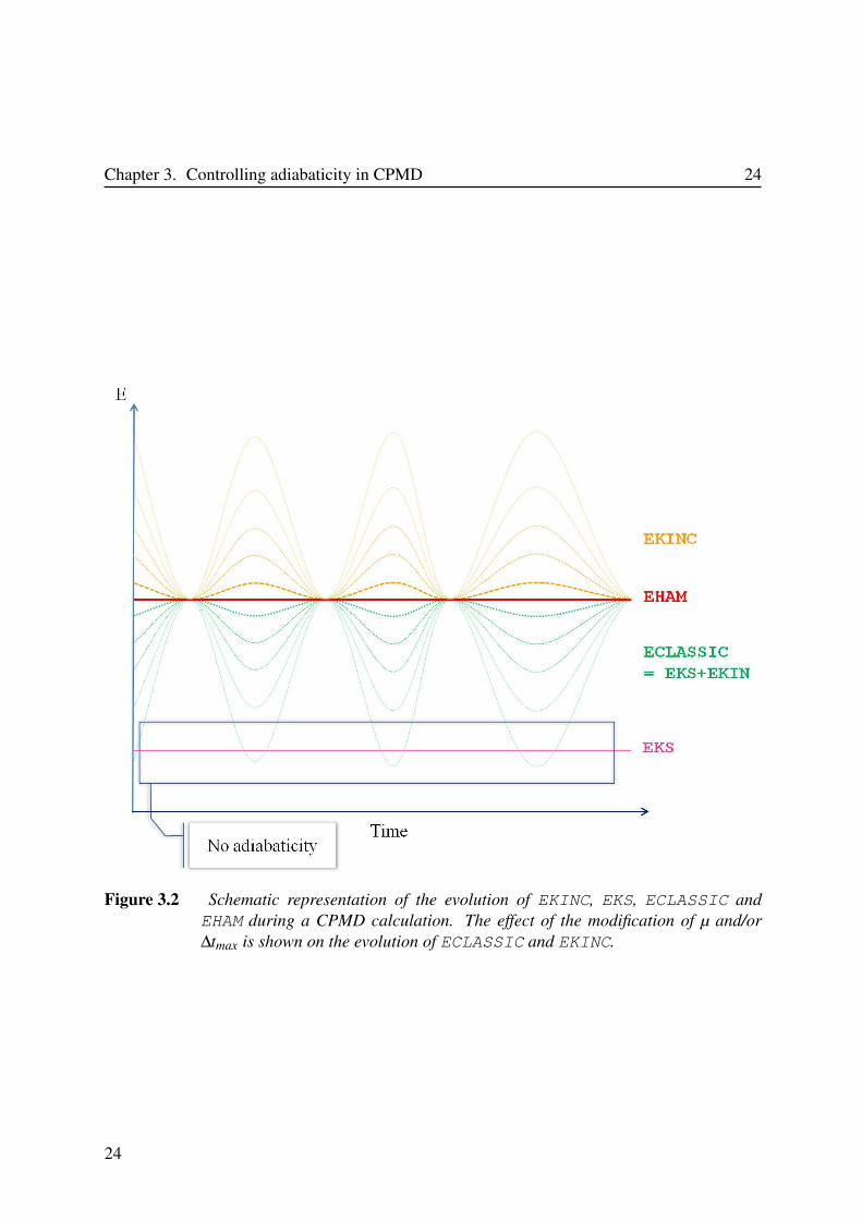
As illustrated in table [Tab. 2.2] in a CPMD calculation the quantities to follow and con-trol are the kinetic energy of the electronic sub-system EKINC, the potential energy from theKohn-Sham equations EKS, the classical first principles energy ECLASSIC, and the conservedenergetic quantity of the CPMD Hamiltonian EHAM. Figure [Fig. 3.2] illustrates the evolutionof these quantities during the dynamics and highlights the effect of the modification of µ and/or∆tmax on the evolution of ECLASSIC and EKINC. EHAM = ECLASSIC + EKINC, then if the variationon ECLASSIC are so important that EKINC interferes with EKS then there is no adiabaticityanymore.

Remark

EKINC should be smaller than 20 % of the difference EHAM - EKS.

23

Chapter 3. Controlling adiabaticity in CPMD 24

Figure 3.2 Schematic representation of the evolution of EKINC, EKS, ECLASSIC and

EHAM during a CPMD calculation. The effect of the modification of µ and/or

∆tmax is shown on the evolution of ECLASSIC and EKINC.

24

Parameters of the Nosé thermostat

For details see references [10–13].

4.1 Nosé thermostats in the CPMD method

When introducing Nosé thermostats (on ions and/or fictitious electrons) the CPMD equations ofmotion [Eq. 3.2 and 3.3] are modified and friction terms are introduced to couple atoms and/orwave-function motions to the thermostats:

MIRI(t) = −∂

∂RI

⟨Ψ|He|Ψ

⟩+

∂

∂RI(constraints) − MI RI xR (4.1)

µiψi(t) = −∂

∂〈ψi|

⟨Ψ|He|Ψ

⟩+

∂

∂〈ψi|(constraints) − µ ψi xe (4.2)

where the last term of each equation, − MIRI xR and − µψixe, are friction terms that couplerespectively atoms and wave-functions dynamics to the thermostats. These frictions terms aregoverned by the variable xR and xe which obey the following equations of motion:

QRxR = 2[

∑I

12

MIR2I −

12

g kb T]

(4.3)

Qexe = 2[

∑i

µ 〈ψi|ψi〉 − Ekin,e

]

(4.4)

where 12 gkbT is the average kinetic energy of the ionic sub-system, g = 3N is the number

of degrees of freedom for the atomic motion in a system with N atoms, kb is the Boltzmannconstant and T the physical temperature of the system. And Ekin,e is the average kinetic energyof the fictitious electronic sub-system. The masses QR and Qe determine the time scale of thethermal fluctuations of the thermostats.

25

Chapter 4. Parameters of the Nosé thermostat 26

4.2 Choosing the parameters

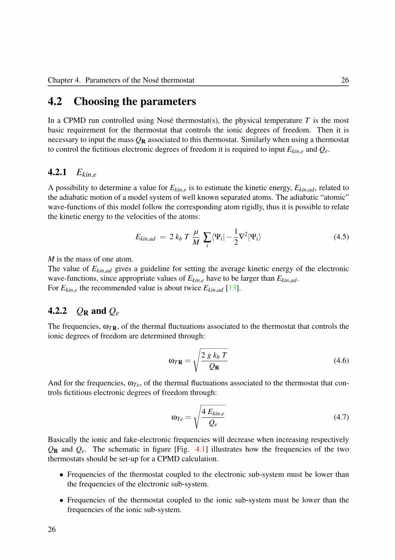
In a CPMD run controlled using Nosé thermostat(s), the physical temperature T is the mostbasic requirement for the thermostat that controls the ionic degrees of freedom. Then it isnecessary to input the mass QR associated to this thermostat. Similarly when using a thermostatto control the fictitious electronic degrees of freedom it is required to input Ekin,e and Qe.

4.2.1 Ekin,e

A possibility to determine a value for Ekin,e is to estimate the kinetic energy, Ekin,ad , related tothe adiabatic motion of a model system of well known separated atoms. The adiabatic “atomic”wave-functions of this model follow the corresponding atom rigidly, thus it is possible to relatethe kinetic energy to the velocities of the atoms:

Ekin,ad = 2 kb Tµ

M∑

i

〈Ψi|−12

∇2|Ψi〉 (4.5)

M is the mass of one atom.The value of Ekin,ad gives a guideline for setting the average kinetic energy of the electronicwave-functions, since appropriate values of Ekin,e have to be larger than Ekin,ad .For Ekin,e the recommended value is about twice Ekin,ad [13].

4.2.2 QR and Qe

The frequencies, ωT R, of the thermal fluctuations associated to the thermostat that controls theionic degrees of freedom are determined through:

ωT R =

√

2 g kb T

QR(4.6)

And for the frequencies, ωTe, of the thermal fluctuations associated to the thermostat that con-trols fictitious electronic degrees of freedom through:

ωTe =

√

4 Ekin,e

Qe

(4.7)

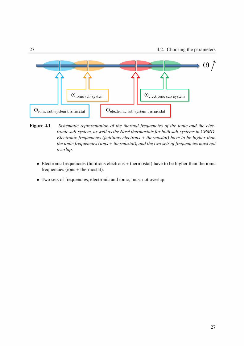
Basically the ionic and fake-electronic frequencies will decrease when increasing respectivelyQR and Qe. The schematic in figure [Fig. 4.1] illustrates how the frequencies of the twothermostats should be set-up for a CPMD calculation.

• Frequencies of the thermostat coupled to the electronic sub-system must be lower thanthe frequencies of the electronic sub-system.

• Frequencies of the thermostat coupled to the ionic sub-system must be lower than thefrequencies of the ionic sub-system.

26

27 4.2. Choosing the parameters

Figure 4.1 Schematic representation of the thermal frequencies of the ionic and the elec-

tronic sub-system, as well as the Nosé thermostats for both sub-systems in CPMD.

Electronic frequencies (fictitious electrons + thermostat) have to be higher than

the ionic frequencies (ions + thermostat), and the two sets of frequencies must not

overlap.

• Electronic frequencies (fictitious electrons + thermostat) have to be higher than the ionicfrequencies (ions + thermostat).

• Two sets of frequencies, electronic and ionic, must not overlap.

27

Bibliography

[1] R. Car and M. Parrinello. Phys. Rev. Lett., 55(22):2471–2474 (1985).

[2] D. Marx and J. Hutter. Mod. Met. Algo. Q. Chem., 1:301–449 (2000).

[3] http://www.cpmd.org.

[4] A. D. Becke and K. E. Edgecombe. J. Chem. Phys., 92:5397–5403 (1990).

[5] A. Savin, A. D. Becke, J. Flad, R. Nesper, H. Preuss, and H. G. von Schnering. Angew.

Chem. Int. Ed. in English, 30(4):409–412 (1991).

[6] A. Savin, O. Jepsen, J. Flad, O. K. Andersen, H. Preuss, and H. G. von Schnering. Angew.

Chem. Int. Ed. in English, 31(2):187–188 (1992).

[7] A. Savin, R. Nesper, S. Wengert, and T. F. Fässler. Angew. Chem. Int. Ed. in English,36(17):1808–1832 (1997).

[8] D. Marx and A. Savin. Angew. Chem. Int. Ed. in English, 36(19):2077–2080 (1997).

[9] G. Pastore, E. Smargiassi, and F. Buda. Phys. Rev. A, 44(10):6334–6347 (1991).

[10] S. Nosé. J. Chem. Phys., 81(1):130511 (1984).

[11] S. Nosé. Mol. Phys., 52(2):255–258 (1984).

[12] W. G. Hoover. Phys. Rev. A, 31(3):1695–1697 (1985).

[13] P. E. Blöchl and M. Parrinello. Phys. Rev. B, 45(16):9413–9416 (1992).

http://www.cpmd.org

This document has been prepared using the Linux operating system and free softwares:The text editor "gVim"The GNU image manipulation program "The Gimp"The WYSIWYG plotting tool "Grace"And the document preparation system "LATEX 2ε".

http://www.vim.org/

http://www.gimp.org/

http://plasma-gate.weizmann.ac.il/Grace/

http://www.latex-project.org/

Basic tutorial to CPMD calculations - Unistra and Parinnello Molecular Dynamics Basic tutorial to...

Documents

Transcript of Basic tutorial to CPMD calculations - Unistra and Parinnello Molecular Dynamics Basic tutorial to...