Geosci. Instrum. Method. Data Syst., 3, 241–245, 2014

www.geosci-instrum-method-data-syst.net/3/241/2014/

doi:10.5194/gi-3-241-2014

© Author(s) 2014. CC Attribution 3.0 License.

Auroral all-sky camera calibration

F. Sigernes1,*, S. E. Holmen1,*, D. Biles2, H. Bjørklund1, X. Chen1,*, M. Dyrland1,*, D. A. Lorentzen1,*, L. Baddeley1,*,

T. Trondsen3, U. Brändström4, E. Trondsen5, B. Lybekk5, J. Moen5, S. Chernouss6, and C. S. Deehr7

1University Centre in Svalbard, Longyearbyen, Norway2Magnetosphere Ionosphere Research Lab, University of New Hampshire, USA3Keo Scientific Ltd, Calgary, Alberta, Canada4Swedish Institute of Space Physics, Kiruna, Sweden5Department of Physics, University of Oslo, Oslo, Norway6Polar Geophysical Institute, Murmansk Region, Apatity, Russia7Geophysical Institute, University of Alaska, Fairbanks, USA*also at: Birkeland Centre for Space Science, University of Bergen, Bergen, Norway

Correspondence to: F. Sigernes (freds@unis.no)

Received: 8 August 2014 – Published in Geosci. Instrum. Method. Data Syst. Discuss.: 1 September 2014

Revised: 28 October 2014 – Accepted: 13 November 2014 – Published: 10 December 2014

Abstract. A two-step procedure to calibrate the spectral sen-

sitivity to visible light of auroral all-sky cameras is outlined.

Center pixel response is obtained by the use of a Lambertian

surface and a standard 45 W tungsten lamp. Screen bright-

ness is regulated by the distance between the lamp and the

screen. All-sky flat-field correction is carried out with a 1 m

diameter integrating sphere. A transparent Lexan dome at the

exit port of the sphere is used to simulate observing con-

ditions at the Kjell Henriksen Observatory (KHO). A cer-

tified portable low brightness source from Keo Scientific Ltd

was used to test the procedure. Transfer lamp certificates in

units of Rayleigh per Ångstrøm (R/Å) are found to be within

a relative error of 2 %. An all-sky camera flat-field correc-

tion method is presented with only 6 required coefficients

per channel.

1 Introduction

During the last decades, numerous ground-based all-sky

cameras have been installed in both hemispheres to moni-

tor aurora and airglow. In the northern hemisphere, the fields

of view of these cameras overlap to cover large sections of

the aurora oval (cf. Akasofu, 1964). The desire to, for exam-

ple, estimate and compare auroral hemispherical power as

measured by satellites (cf. Zhang and Paxton, 2008) requires

unified and accurate calibration routines (Brändström et al.,

2012) to quantify the radiance in photometric units (Hunten

et al., 1956). This paper presents a two-step procedure to cal-

ibrate to sensitivity the all-sky cameras at the Kjell Henriksen

Observatory (KHO).

2 Experimental setup

The calibration tools are shown in Fig. 1. The fixed imag-

ing compact spectrograph (FICS) is mounted on a height-

adjustable table. The table can be moved on rails towards

the Lambertian screen. The entrance optics of FICS is a 22◦

field-of-view-fused silica fibre bundle. The spectrograph is

made by ORIEL (model 77443). It uses a concave holo-

graphic grating (230 grooves/mm). The nominal spectral

range is 4000–11 000 Å, and the bandpass is approximately

80 Å with the 100 µm wide entrance slit. The detector is a 16

bit dynamic range thermoelectric cooled CCD camera from

the company Andor (model DU 420A-OE). Our main cal-

ibration source, the 45 W tungsten lamp from Oriel (s/n 7-

1867), is also mounted on the table. The lamp is a traceable

National Institute of Standards (NIST) source. The lamp cer-

tificate is listed in Table 1. Both the Lambertian screen (SRT-

99-180) and the 1 m diameter integrating sphere (CSTM-LR-

40) are made by the company Labsphere. Note that in Fig. 1,

the spectrograph is set up to measure the output of the inte-

grating sphere.

Published by Copernicus Publications on behalf of the European Geosciences Union.

242 F. Sigernes et al.: Auroral all-sky camera calibration

13

1

2

Figure 1. Experimental setup at the UNIS calibration lab. Panel (A): (1) Labsphere 1m 3

diameter low light level integrating sphere, (2) source sphere with tungsten lamp, (3) 45W 4

tungsten lamp, (4) FICS fiber bundle probe, (5) FICS, (6) rail road, (7) Keo Alcor-RC low 5

light source, (8) Lambertian screen, (9) height adjustable table on rails, (10) table jacks, and 6

(11) rotary probe mount. Panel (B): Keo Alcor-RC low light source. 7

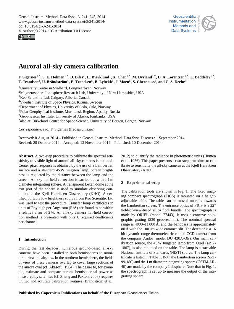
Figure 1. Experimental setup at the UNIS calibration lab. (a) (1)

Labsphere 1m diameter low light level integrating sphere, (2) source

sphere with tungsten lamp, (3) 45W tungsten lamp, (4) FICS fiber

bundle probe, (5) FICS, (6) rail road, (7) Keo Alcor-RC low light

source, (8) Lambertian screen, (9) height adjustable table on rails,

(10) table jacks and (11) rotary probe mount. (b) Keo Alcor-RC low

light source.

Table 1. Oriel 45 W tungsten lamp certificate (s/n 7-1867). The

spectral irradiance values are measured at a distance of z0 = 0.5 m.

Irradiance Irradiance

Wavelength M0(λ) M0(λ)

λ [Å] [mW m−2 nm−1] [#photons cm−2 s−1 Å−1]

4000 0.79670 1.60221× 1010

4500 1.71388 3.87755× 1010

5000 2.99143 7.51994× 1010

5550 4.65315 1.29839× 1011

6000 6.04915 1.82478× 1011

6546 7.64049 2.51456× 1011

7000 8.76666 3.08530× 1011

8000 11.1985 4.50416× 1011

The integrating sphere is modified by including a trans-

parent dome at the exit port and a baffle to block light from

the source sphere. A sketch of the modifications is shown in

Fig. 2. The dome is made of the same material (Lexan) and

thickness (5 mm) as the domes at the KHO. The all-sky cam-

eras should be inserted into the dome in order to fill the total

field of view of 180◦. The baffle acts as a moon blocker. The

net result is that observational and calibration conditions are

the same for all optical instruments housed at the KHO.

The FICS is sensitivity-calibrated by the use of the Lam-

bertian screen and the 45 W tungsten lamp. The distance and

angle between the screen and the lamp regulate the bright-

ness of the screen. This well-known method of calibrating

narrow field-of-view instruments is described in detail by

Sigernes et al. (2007).

14

1 Figure 2. Sketch of modification to the 1m diameter integrating sphere: (1) Labsphere CSTM-2 LR-40, (2) transparent Lexan dome, (3) baffle, (4) transparent diffusor, (5) adjustable 3 aperture, (6) source sphere, (7) tungsten lamp, and (8) instrument with all-sky lens. Red 4 arrows and lines indicate the effect of multiple scattering inside the sphere. 5

Figure 2. Sketch of modification to the 1m diameter integrating

sphere: (1) Labsphere CSTM-LR-40, (2) transparent Lexan dome,

(3) baffle, (4) transparent diffusor, (5) adjustable aperture, (6) source

sphere, (7) tungsten lamp and (8) instrument with all-sky lens. Red

arrows and lines indicate the effect of multiple scattering inside the

sphere.

15

1 Figure 3. Absolute and wavelength calibration of the FICS. The line spectrum in red is from a 2

mercury vapour lamp supplied by Edmund Optics Ltd (SN K60-908). The solid black spectra 3

are from the Keo Alcor-RC certificate. The corresponding black dotted lines are spectra 4

measured by the FICS. The spectrum of the integrating sphere is plotted in blue. 5

6

7

Figure 3. Absolute and wavelength calibration of the FICS. The

line spectrum in red is from a mercury vapor lamp supplied by Ed-

mund Optics Ltd (SN K60-908). The solid black spectra are from

the Keo Alcor-RC certificate. The corresponding black dotted lines

are spectra measured by the FICS. The spectrum of the integrating

sphere is plotted in blue.

3 Test and tuning of calibration tools

A mobile low light source made by the company Keo Sci-

entific is used to test the new calibration method. The head

unit of the Keo Alcor-RC low brightness source (s/n 10113)

is visible in Fig. 1. It contains a 100 W tungsten lamp, aper-

ture wheels and diffusors to attenuate the brightness of the

opal output surface. The source is certified by the National

Research Council of Canada (NRC).

The FICS fiber probe is mounted head-on to the center of

the output surface of the Keo-Alcor-RC source. The field of

Geosci. Instrum. Method. Data Syst., 3, 241–245, 2014 www.geosci-instrum-method-data-syst.net/3/241/2014/

F. Sigernes et al.: Auroral all-sky camera calibration 243

Table 2. The difference in spectral calibration between UNIS – FICS and NRC of the Keo Alcor-RC low brightness source as a function of

aperture. All numbers are in units of %.

Keo Alcor – RC aperture 25.9 19.1 13.0 10.1 6.62 5.24 3.26 2.05 1.08

Difference 2.00 1.56 1.41 0.40 1.42 0.04 0.90 0.26 1.96

Table 3. Fish-eye mapping functions. F is the effective focal length

of the lens, and θ is the angle to the optical axis.

Type Fish-eye mapping function

Linear scaled R = f × θ

Orthographic R = f × sin(θ)

Equal area R = 2× f × sin(θ/2)

Stereographic R = 2× f × tan(θ/2)

view of the probe is then within a 1 cm diameter spot size

of the diffuse surface. The setup is compatible to the spec-

tral irradiance measured by Gaertner (2013). Figure 3 shows

the measured FICS spectra and the corresponding certified

spectra from NRC as a function of aperture setting. The Keo

Alcor-RC aperture is given in units of percentage. 100 % is

maximum brightness, while 10 % means that the brightness

is one tenth of maximum.

The percent of error between the measured integrated

FICS spectra and the NRC certificate is used to quantify the

relative difference in the calibrations. The results are listed in

Table 2 as a function of Keo aperture. Note that the relative

errors are less than or equal to 2 %.

The next step in the test is to move the FICS fiber probe

to the center of the Labsphere integrating sphere output port

and tune the aperture of the source sphere down to a level that

corresponds to the one tenth aperture brightness of the Alcor-

RC source. The spectral radiance is then below the threshold

of ∼ 1 kR/Å, which is close to the intensity range of magni-

tude for auroras and airglow as indicated by the blue-colored

spectrum in Fig. 3.

4 Basic camera equations

This section derives the equations needed for calibration of

multiple wavelength filtered all-sky cameras. The experi-

mental setup is as sketched in Fig. 2 using the integrating

sphere as source. The type of filters used depends on center

wavelength λc, bandpass BP and transmission T . The most

traditional one is the Fabry–Perot filter design, where paral-

lel transparent glass plates create interference due to multiple

reflections between the plates.

The raw data counts of the camera at pixel position (x,y)

are given as an integral over wavelength:

u=

∫B(λ) · S(λ)dλ, [cts], (1)

16

1

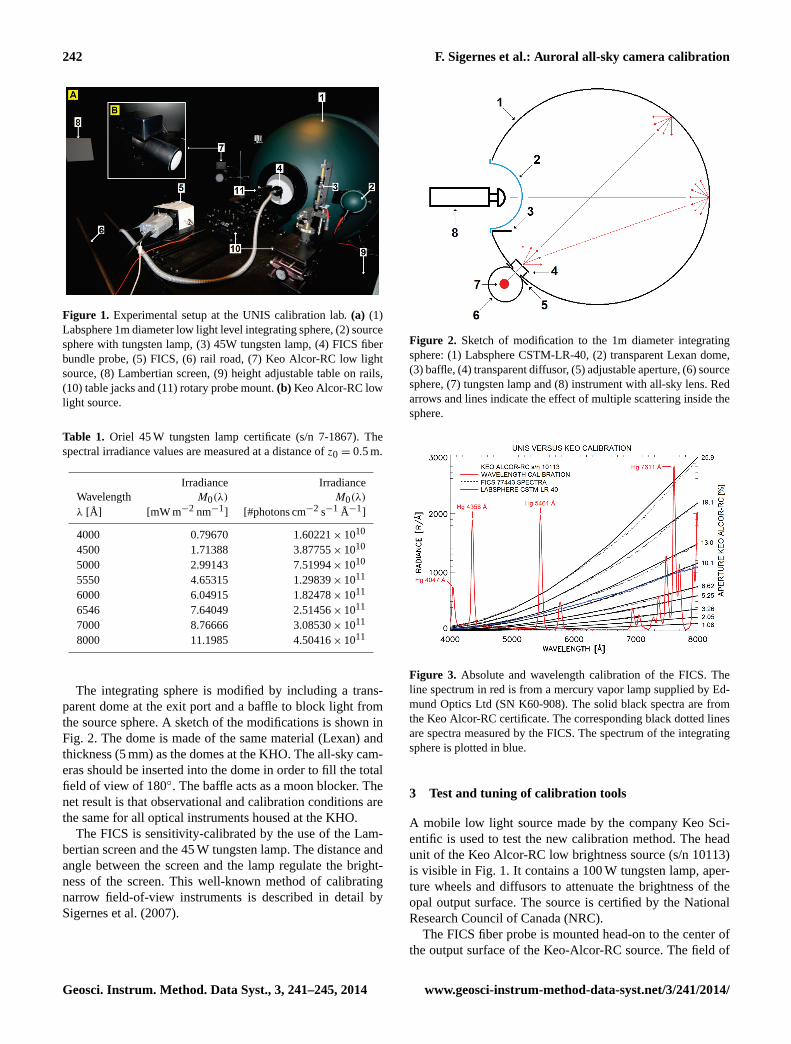
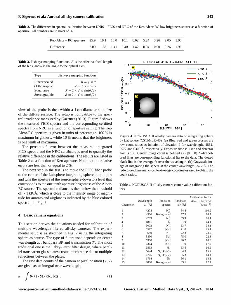
Figure 4. NORUSCA II all-sky camera data of integrating sphere by Labsphere (CSTM-LR-2

40). Panel (A): Blue, red and green crosses are raw count ratios as function of elevation θ for 3

wavelengths 4861, 5577 and 6300 Å, respectively. Exposure time was 1 second and detector 4

gain is 100. Center image count is defined as ( 0)u θ = . Solid colored lines are corresponding 5

functional fits to the data. The dotted black line is the average fit over wavelength. Panel (B): 6

Grayscale image of integrating sphere at center wavelength 5577 Å. The red colored line 7

marks center to edge coordinates used to obtain the count ratios. 8

Figure 4. NORUSCA II all-sky camera data of integrating sphere

by Labsphere (CSTM-LR-40). (a) Blue, red and green crosses are

raw count ratios as function of elevation θ for wavelengths 4861,

5577 and 6300 Å, respectively. Exposure time is 1 sec and detector

gain is 100. Center image count is defined as u(θ = 0). Solid col-

ored lines are corresponding functional fits to the data. The dotted

black line is the average fit over the wavelength. (b) Grayscale im-

age of integrating the sphere at the center wavelength 5577 Å. The

red-colored line marks center-to-edge coordinates used to obtain the

count ratios.

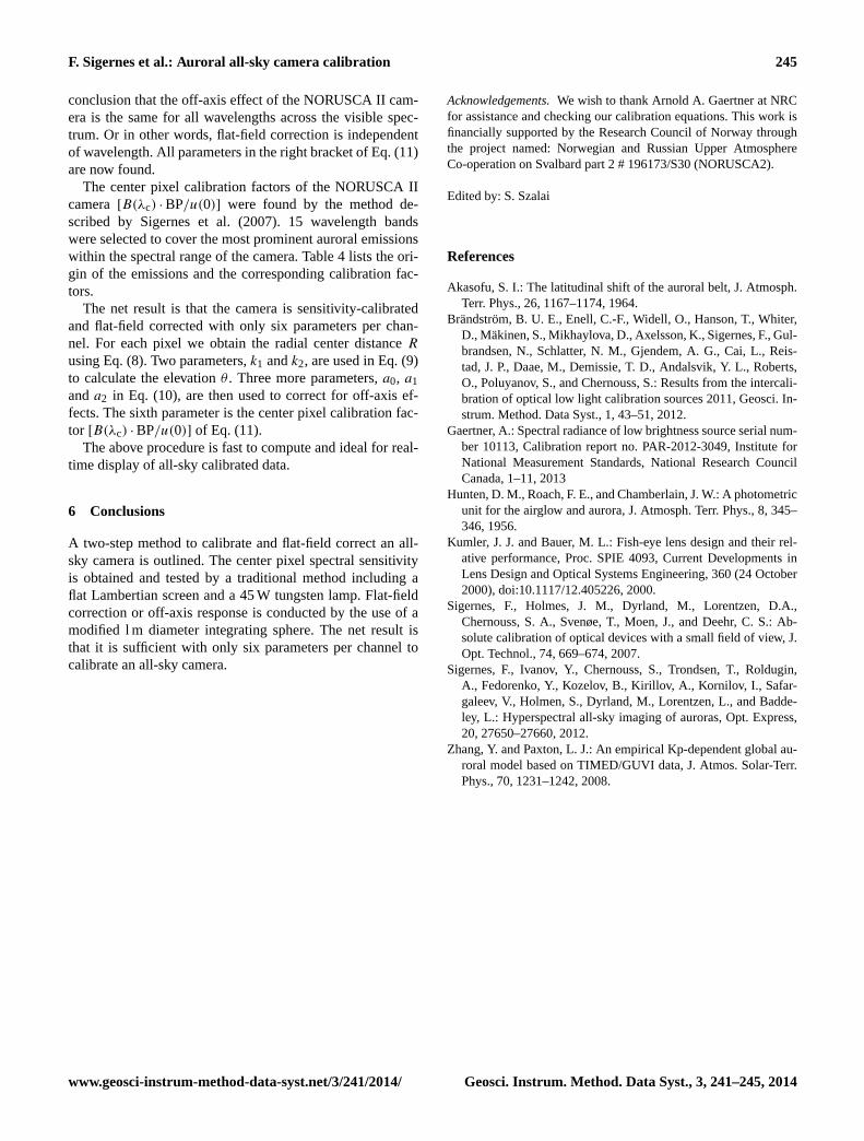
Table 4. NORUSCA II all-sky camera center value calibration fac-

tors.

Calibration factor

Wavelength Emission Bandpass B(λc) · BP/u(0)

Channel # λc [Å] species BP [Å] [R cts−1]

1 4278 N+2

54.4 110.2

2 4500 Background 57.3 88.7

3 4709 N+2

59.9 60.1

4 4861 Hβ 61.9 44.4

5 5002 NII 63.7 38.1

6 5577 [OI] 71.0 25.1

7 5680 NII 72.3 23.7

8 5890 NaI 75.0 22.3

9 6300 [OI] 80.2 18.8

10 6364 [OI] 81.0 17.7

11 6563 Hα 83.5 16.6

12 6624 N21P(6-3) 84.3 15.7

13 6705 N21P(5-2) 85.3 14.4

14 6764 N2 86.1 14.1

15 7000 Background 89.1 12.4

www.geosci-instrum-method-data-syst.net/3/241/2014/ Geosci. Instrum. Method. Data Syst., 3, 241–245, 2014

244 F. Sigernes et al.: Auroral all-sky camera calibration

where S is defined as the spectral responsivity and B is the

source spectrum in absolute units. The wavelength depen-

dency of the spectral responsivity is assumed to be propor-

tional to the transmission of the filter:

S(λ)≈ ε · T (λ).[cts R−1]. (2)

If the source B, lens transmissions and detector sensitivity

vary slowly in the wavelength interval 1λ, then Eq. (1) be-

comes

u= B(λc) · ε ·

∫T (λ)dλ= B(λc) · ε ·A, (3)

where A is the area of the filter transmission curve. It is as-

sumed that T is narrow and triangular in shape. Then

A=

∫T (λ)dλ≈ Tm ·BP, (4)

where Tmis the peak transmission of the filter at λ= λc. Fur-

thermore, the spectral radiance of a discrete auroral emission

line at wavelength λc is defined as

Ja(λ)≡ J · δ(λ− λc)[R/Å], (5)

where δ is the Kronecker delta. The number of auroral raw

data counts is then

ua =∫Ja(λ) · S(λ)dλ=

∫J · δ(λ− λc) · ε · T (λ)dλ

= J · ε ·∫T (λ) · δ(λ− λc)dλ= J · ε · Tm.

(6)

Finally, from Eqs. (3), (4) and (6),

J = ua×

[B(λc) ·BP

u

].[R]. (7)

Note that Eq. (7) is only valid when the transmission profile

of the filter is narrow and triangular.

The (B/u) factor for each pixel in the all-sky image must

be examined further. Let us introduce the radial center pixel

distance, R, of a point in the image plane defined as

R ≡

√(x− xc)2+ (y− yc)2, (8)

where (xc,yc) are the center pixel coordinates. The relation

between R and the zenith angle θ is known as the radial map-

ping function. Table 3 lists typical fish-eye mapping func-

tions. In a more general form, Kumler and Bauer (2000) sug-

gested that circular image fish-eye lenses have mapping func-

tions equal to

R = k1 · f · sin(k2 · θ).[mm]. (9)

For the hyperspectral all-sky camera at KHO named NOR-

USCA II (Sigernes et al., 2012), the coefficients are f =

3.5 mm, k1 = 1.2 and k2 = 0.83, using known star positions

as input data.

The radiance B of the integrating sphere is per definition

uniform in all directions of θ , and (x, y) points with equal R

should, due to symmetry, have the same raw data count rate

of u. As a consequence, it is useful to transform our (x,y)

coordinates to (R,θ) coordinates with Eqs. (8) and (9). It

must be emphasized that the above assumption is for an ideal

conditioned sphere with no deterioration of the inside coating

(Barium sulfate) over time. A functional fit to the data for

each wavelength channel may then be found as

u= u(θ)≈ u(0) · [a0 cos(a1 · θ)+ a2]. (10)

A 3rd degree polynomial fit may also be used. The final form

of Eq. (7) becomes

J = ua×

[B(λc) ·BP

u(0)

]×

[1

a0 cos(a1 · θ)+ a2

]. (11)

Note that the left bracket in Eq. (11) only requires center

(θ = 0) values u, while the right bracket describes the off-

axis (θ>0) behavior of the camera. It is known as flat-field

correction of image ua.

Based on the above equations, we propose the calibration

to be undertaken in two steps. The first step is to find the co-

efficients a0, a1 and a2 by using the integrating sphere. The

second step is to measure the center pixel area counts of u(0)

by using the Lambertian screen setup instead of the integrat-

ing sphere. The screen to lamp distance z is very useful to

regulate screen brightness to the same order of magnitude as

that expected during sampling of the aurora. The exposure

time and gain settings are identical for both the calibration

and normal dark-sky operation of the cameras. The latter also

cancels out any effect due to nonlinear behavior of count lev-

els versus exposure time. The spectral radiance of the screen

is given as

B(λ)=

(4ρ

106

)×M0(λ)×

(z0

z

)2

× cosα.[R/Å]. (12)

M0(λ) is the known irradiance (certificate) of the lamp in

units of [#photons cm−2 s−1 Å−1], initially obtained at a dis-

tance of zo = 0.5 m (see Table 1). The diffuse reflectance fac-

tor ρ of the screen is nearly constant (ρ = 0.98) throughout

the visible and near infrared regions of the spectrum. The an-

gle α is between the screen and the tungsten lamp (α = 0).

5 Results

Three 1 sec exposures at center wavelengths 4861, 5577 and

6300 Å of the integrating sphere were used to obtain the raw

count ratio u(θ)/u(0) for the NORUSCA II camera. The re-

sults are shown in Fig. 4. A functional LMFIT in IDL (In-

teractive Data Language) based on the Levenberg-Marquardt

algorithm results in coefficients a0 = 0.38, a1 = 1.29 and

a2 = 0.63 (see Eq. 10). Note that in our case there is no sig-

nificant difference in shape and level of the raw count ra-

tio between the three wavelength channels. This leads to the

Geosci. Instrum. Method. Data Syst., 3, 241–245, 2014 www.geosci-instrum-method-data-syst.net/3/241/2014/

F. Sigernes et al.: Auroral all-sky camera calibration 245

conclusion that the off-axis effect of the NORUSCA II cam-

era is the same for all wavelengths across the visible spec-

trum. Or in other words, flat-field correction is independent

of wavelength. All parameters in the right bracket of Eq. (11)

are now found.

The center pixel calibration factors of the NORUSCA II

camera [B(λc) ·BP/u(0)] were found by the method de-

scribed by Sigernes et al. (2007). 15 wavelength bands

were selected to cover the most prominent auroral emissions

within the spectral range of the camera. Table 4 lists the ori-

gin of the emissions and the corresponding calibration fac-

tors.

The net result is that the camera is sensitivity-calibrated

and flat-field corrected with only six parameters per chan-

nel. For each pixel we obtain the radial center distance R

using Eq. (8). Two parameters, k1 and k2, are used in Eq. (9)

to calculate the elevation θ . Three more parameters, a0, a1

and a2 in Eq. (10), are then used to correct for off-axis ef-

fects. The sixth parameter is the center pixel calibration fac-

tor [B(λc) ·BP/u(0)] of Eq. (11).

The above procedure is fast to compute and ideal for real-

time display of all-sky calibrated data.

6 Conclusions

A two-step method to calibrate and flat-field correct an all-

sky camera is outlined. The center pixel spectral sensitivity

is obtained and tested by a traditional method including a

flat Lambertian screen and a 45 W tungsten lamp. Flat-field

correction or off-axis response is conducted by the use of a

modified l m diameter integrating sphere. The net result is

that it is sufficient with only six parameters per channel to

calibrate an all-sky camera.

Acknowledgements. We wish to thank Arnold A. Gaertner at NRC

for assistance and checking our calibration equations. This work is

financially supported by the Research Council of Norway through

the project named: Norwegian and Russian Upper Atmosphere

Co-operation on Svalbard part 2 # 196173/S30 (NORUSCA2).

Edited by: S. Szalai

References

Akasofu, S. I.: The latitudinal shift of the auroral belt, J. Atmosph.

Terr. Phys., 26, 1167–1174, 1964.

Brändström, B. U. E., Enell, C.-F., Widell, O., Hanson, T., Whiter,

D., Mäkinen, S., Mikhaylova, D., Axelsson, K., Sigernes, F., Gul-

brandsen, N., Schlatter, N. M., Gjendem, A. G., Cai, L., Reis-

tad, J. P., Daae, M., Demissie, T. D., Andalsvik, Y. L., Roberts,

O., Poluyanov, S., and Chernouss, S.: Results from the intercali-

bration of optical low light calibration sources 2011, Geosci. In-

strum. Method. Data Syst., 1, 43–51, 2012.

Gaertner, A.: Spectral radiance of low brightness source serial num-

ber 10113, Calibration report no. PAR-2012-3049, Institute for

National Measurement Standards, National Research Council

Canada, 1–11, 2013

Hunten, D. M., Roach, F. E., and Chamberlain, J. W.: A photometric

unit for the airglow and aurora, J. Atmosph. Terr. Phys., 8, 345–

346, 1956.

Kumler, J. J. and Bauer, M. L.: Fish-eye lens design and their rel-

ative performance, Proc. SPIE 4093, Current Developments in

Lens Design and Optical Systems Engineering, 360 (24 October

2000), doi:10.1117/12.405226, 2000.

Sigernes, F., Holmes, J. M., Dyrland, M., Lorentzen, D.A.,

Chernouss, S. A., Svenøe, T., Moen, J., and Deehr, C. S.: Ab-

solute calibration of optical devices with a small field of view, J.

Opt. Technol., 74, 669–674, 2007.

Sigernes, F., Ivanov, Y., Chernouss, S., Trondsen, T., Roldugin,

A., Fedorenko, Y., Kozelov, B., Kirillov, A., Kornilov, I., Safar-

galeev, V., Holmen, S., Dyrland, M., Lorentzen, L., and Badde-

ley, L.: Hyperspectral all-sky imaging of auroras, Opt. Express,

20, 27650–27660, 2012.

Zhang, Y. and Paxton, L. J.: An empirical Kp-dependent global au-

roral model based on TIMED/GUVI data, J. Atmos. Solar-Terr.

Phys., 70, 1231–1242, 2008.

www.geosci-instrum-method-data-syst.net/3/241/2014/ Geosci. Instrum. Method. Data Syst., 3, 241–245, 2014