
ANALYSIS TOOLS FOR THE DESIGN OF ALUMINIUM EXTRUSION DIES · Summary The aluminium extrusion...
164
ANALYSIS TOOLS FOR THE DESIGN OF ALUMINIUM EXTRUSION DIES A.J. Koopman
Transcript of ANALYSIS TOOLS FOR THE DESIGN OF ALUMINIUM EXTRUSION DIES · Summary The aluminium extrusion...

ANALYSIS TOOLS FOR THE DESIGN OF
ALUMINIUM EXTRUSION DIES
A.J. Koopman
This research was carried out within the framework of the Simalex project,which was initiated by Boalgroup in De Lier.
De promotiecommissie is als volgt samengesteld:
Voorzitter en secretaris:Prof.dr.ir. F. Eising Universiteit TwentePromotoren:Prof. dr. ir. J. Huetink Universiteit TwenteProf. dr. ir. F.J.A.M. van Houten Universiteit TwenteAssisent Promotor :Dr.ir. H.J.M Geijselaers Universiteit TwenteLeden:Prof. dr.-Ing. A. E. Tekkaya Universiteit DortmundProf. dr. ir. F. Soetens Technische Universiteit EindhovenProf. dr. ir. D.J. Schipper Universiteit TwenteProf. dr.ir. R. Akkerman Universiteit Twentedr. R.M.J van Damme Universiteit Twente
Analysis tools for the design of aluminium extrusion diesKoopman, Albertus JohannesPhD thesis, University of Twente, Enschede, The NetherlandsMarch 2008
ISBN 978-90-9024381-8Subject headings: Flow front tracking, Simulation based Die design
Copyright c©2009 by A.J. Koopman, Enschede, The NetherlandsPrinted by Laseline, Hengelo, The Netherlands
ANALYSIS TOOLS FOR THE DESIGN OF
ALUMINIUM EXTRUSION DIES
PROEFSCHRIFT
ter verkrijging vande graad van doctor aan de Universiteit Twente,
op gezag van de rector magnificus,prof. dr. H. Brinksma,
volgens besluit van het College voor Promotiesin het openbaar te verdedigen
op donderdag 11 juni 2009 om 15.00 uur
door
Albertus Johannes Koopman
geboren op 22 november 1976
te Brederwiede

Dit proefschrift is goedgekeurd door de promotoren:Prof. dr. ir. J. HuetinkProf. dr. ir. F.J.A.M. van Houtenen de assistent promotordr. ir. H.J.M. Geijselears
Summary
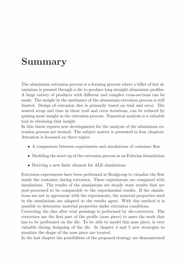
The aluminium extrusion process is a forming process where a billet of hot al-uminium is pressed through a die to produce long straight aluminium profiles.A large variety of products with different and complex cross-sections can bemade. The insight in the mechanics of the aluminium extrusion process is stilllimited. Design of extrusion dies is primarily based on trial and error. Thewasted scrap and time in these trail and error iterations, can be reduced bygaining more insight in the extrusion process. Numerical analysis is a valuabletool in obtaining that insight.In this thesis reports new developments for the analysis of the aluminium ex-trusion process are treated. The subject matter is presented in four chapters.Attention is focussed on three topics:
• A comparison between experiments and simulations of container flow
• Modeling the start-up of the extrusion process in an Eulerian formulation
• Deriving a new finite element for ALE simulations
Extrusion experiments have been performed at Boalgroup to visualize the flowinside the container during extrusion. These experiments are compared withsimulations. The results of the simulations are steady state results that arepost-processed to be comparable to the experimental results. If the simula-tions are not in agreement with the experiments, the material properties usedin the simulations are adapted so the results agree. With this method it ispossible to determine material properties under extrusion conditions.Correcting the dies after trial pressings is performed by die-correctors. Thecorrectors use the first part of the profile (nose piece) to asses the work thathas to be performed on the die. To be able to model this nose piece, is veryvaluable during designing of the die. In chapter 4 and 5 new strategies tosimulate the shape of the nose piece are treated.In the last chapter the possibilities of the proposed strategy are demonstrated

vi
on a porthole die for a tube. The simulated nose piece is in very good agree-ment with the experimental results.
Samenvatting
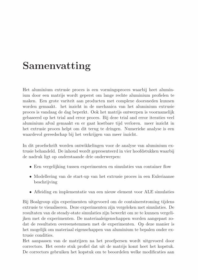
Het aluminium extrusie proces is een vormingsproces waarbij heet alumin-ium door een matrijs wordt geperst om lange rechte aluminium profielen temaken. Een grote variteit aan producten met complexe doorsneden kunnenworden gemaakt. het inzicht in de mechanica van het aluminium extrusieproces is vandaag de dag beperkt. Ook het matrijs ontwerpen is voornamelijkgebaseerd op het trial and error proces. Bij deze trial and error iteraties veelaluminium afval gemaakt en er gaat kostbare tijd verloren. meer inzicht inhet extrusie proces helpt om dit terug te dringen. Numerieke analyse is eenwaardevol gereedschap bij het verkrijgen van meer inzicht.
In dit proefschrift worden ontwikkelingen voor de analyse van aluminium ex-trusie behandeld. De inhoud wordt gepresenteerd in vier hoofdstukken waarbijde nadruk ligt op onderstaande drie onderwerpen:
• Een vergelijking tussen experimenten en simulaties van container flow
• Modellering van de start-up van het extrusie proces in een Euleriaansebeschrijving
• Afleiding en implementatie van een nieuw element voor ALE simulaties
Bij Boalgroup zijn experimenten uitgevoerd om de containerstroming tijdensextrusie te visualiseren. Deze experimenten zijn vergeleken met simulaties. Deresultaten van de steady-state simulaties zijn bewerkt om ze te kunnen vergeli-jken met de experimenten. De materiaaleigenschappen worden aangepast zo-dat de resultaten overeenstemmen met de experimenten. Op deze manier ishet mogelijk om materiaal eigenschappen van aluminium te bepalen onder ex-trusie condities.Het aanpassen van de matrijzen na het proefpersen wordt uitgevoerd doorcorrectors. Het eerste stuk profiel dat uit de matrijs komt heet het kopstuk.De correctors gebruiken het kopstuk om te beoordelen welke modificaties aan

viii
de matrijs noodzakelijk zijn. Om vorm van het kopstuk te kunnen voorspellenis van grote waarde tijdens het matrijs ontwerp. In hoofdstukken 4 en 5 wordteen nieuwe methode behandeld om de vorm van het kopstuk te bepalen.In het laatste hoofdstuk worden, aan de hand van een vergelijking tussen ex-periment en simulatie van de extrusie van een buis, de mogelijkheden getoondvan de voorgestelde methode. De vorm van het kopstuk voorspeld met demethode komt goed overeen met de vorm van het kopstuk uit het experiment.
Contents
Summary v
Samenvatting vii
Contents ix
1 Introduction 1
1.1 Aluminium extrusion process . . . . . . . . . . . . . . . . . . . 2
1.1.1 Flow related defects in aluminium extrusion . . . . . . . 4
1.2 Example: feeder hole area . . . . . . . . . . . . . . . . . . . . . 5
1.3 Numerical simulations of aluminium extrusion . . . . . . . . . . 6
1.4 Outline of the thesis . . . . . . . . . . . . . . . . . . . . . . . . 7
2 Finite element analysis of aluminium extrusion 11
2.1 Introduction . . . . . . . . . . . . . . . . . . . . . . . . . . . . . 11
2.2 Different FEM formulations . . . . . . . . . . . . . . . . . . . . 13
2.2.1 Lagrangian formulation . . . . . . . . . . . . . . . . . . 13
2.2.2 Eulerian formulation . . . . . . . . . . . . . . . . . . . . 14
2.2.3 ALE formulation . . . . . . . . . . . . . . . . . . . . . . 14
2.3 Arbitrary Lagrangian Eulerian formulation . . . . . . . . . . . 15
2.3.1 Strong form . . . . . . . . . . . . . . . . . . . . . . . . . 16
2.3.2 Weak form . . . . . . . . . . . . . . . . . . . . . . . . . 17
2.3.3 Coupled and semi-coupled ALE . . . . . . . . . . . . . . 17
2.3.4 Material increment . . . . . . . . . . . . . . . . . . . . . 20
2.3.5 Convective increment . . . . . . . . . . . . . . . . . . . 23
2.3.6 Convection scheme . . . . . . . . . . . . . . . . . . . . . 24
2.4 Modeling aluminium extrusion . . . . . . . . . . . . . . . . . . 28
2.4.1 Pre-processing . . . . . . . . . . . . . . . . . . . . . . . 28
2.4.2 Equivalent bearing corner . . . . . . . . . . . . . . . . . 32
ix
x
3 Front line tracking in a steady state flow 41
3.1 Introduction . . . . . . . . . . . . . . . . . . . . . . . . . . . . . 41
3.2 Experiments . . . . . . . . . . . . . . . . . . . . . . . . . . . . . 41
3.3 Theoretical outline for front line tracking demonstrated on New-tonian viscous flow . . . . . . . . . . . . . . . . . . . . . . . . . 44
3.3.1 Viscous flow in a long parallel channel . . . . . . . . . . 46
3.3.2 Solutions for a discretized velocity field . . . . . . . . . 48
3.3.3 Comparison of analytical and discretized results . . . . 49
3.4 Post-processing FEM results . . . . . . . . . . . . . . . . . . . . 49
3.4.1 Post-processing . . . . . . . . . . . . . . . . . . . . . . . 50
3.4.2 A SUPG stabilization for determining front lines . . . . 50
3.4.3 Determination of the upwind parameter α . . . . . . . . 51
3.4.4 Assembly of front lines for comparison . . . . . . . . . . 54
3.5 Simulations of container flow in aluminium extrusion . . . . . . 56
3.5.1 material properties . . . . . . . . . . . . . . . . . . . . . 56
3.5.2 FEM modeling . . . . . . . . . . . . . . . . . . . . . . . 57
3.6 Comparison . . . . . . . . . . . . . . . . . . . . . . . . . . . . . 58
3.7 Concluding remarks . . . . . . . . . . . . . . . . . . . . . . . . 59
4 Flow front tracking 61
4.1 Flow front tracking algorithms . . . . . . . . . . . . . . . . . . 62
4.2 Original coordinate tracking . . . . . . . . . . . . . . . . . . . . 63
4.3 Convection algorithm . . . . . . . . . . . . . . . . . . . . . . . . 64
4.3.1 Weighted local and global smoothing for nodal values . 64
4.3.2 2D Rigid body flows . . . . . . . . . . . . . . . . . . . . 67
4.3.3 Single vortex flow field . . . . . . . . . . . . . . . . . . 68
4.4 Numerical model . . . . . . . . . . . . . . . . . . . . . . . . . . 71
4.4.1 Interface description for extrusion . . . . . . . . . . . . 71
4.4.2 Permeable boundary conditions . . . . . . . . . . . . . . 72
4.4.3 Modeling the pseudo material . . . . . . . . . . . . . . . 74
4.4.4 Flow front regularization . . . . . . . . . . . . . . . . . 76
4.5 2D filling of Die cavity . . . . . . . . . . . . . . . . . . . . . . . 77
4.5.1 Results of 2D die filling . . . . . . . . . . . . . . . . . . 79
4.6 3D Filling of die cavity . . . . . . . . . . . . . . . . . . . . . . 83
4.6.1 FEM model . . . . . . . . . . . . . . . . . . . . . . . . . 84
4.6.2 Results . . . . . . . . . . . . . . . . . . . . . . . . . . . 87
4.6.3 3D Volume conservation . . . . . . . . . . . . . . . . . . 90
4.6.4 Visual comparison . . . . . . . . . . . . . . . . . . . . . 91
4.7 Conclusions . . . . . . . . . . . . . . . . . . . . . . . . . . . . . 92
Contents xi
5 A mixed finite element with original coordinate tracking 95
5.1 Theoretical outline . . . . . . . . . . . . . . . . . . . . . . . . . 965.1.1 Strong formulation . . . . . . . . . . . . . . . . . . . . . 965.1.2 Weak formulation . . . . . . . . . . . . . . . . . . . . . 97
5.2 FEM discretisation . . . . . . . . . . . . . . . . . . . . . . . . 975.3 Convection . . . . . . . . . . . . . . . . . . . . . . . . . . . . . 100
5.3.1 Courant number for triangular elements . . . . . . . . . 1015.3.2 Rigid rotation & Single vortex flow field . . . . . . . . . 104
5.4 Implementation in DiekA . . . . . . . . . . . . . . . . . . . . . 1075.4.1 Incremental-iterative update . . . . . . . . . . . . . . . 1075.4.2 Updated Lagrangian . . . . . . . . . . . . . . . . . . . . 1075.4.3 Implementation for ALE . . . . . . . . . . . . . . . . . . 108
5.5 Updated Lagrangian application: Tube expansion . . . . . . . . 1105.5.1 Analytical . . . . . . . . . . . . . . . . . . . . . . . . . . 1115.5.2 Numerical . . . . . . . . . . . . . . . . . . . . . . . . . . 112
5.6 Eulerian example: 2D Filling . . . . . . . . . . . . . . . . . . . 1145.6.1 Flow front and volume conservation of 2D filling . . . . 1155.6.2 Extrusion force for 2D filling . . . . . . . . . . . . . . . 116
6 Two applications 119
6.1 Container flow . . . . . . . . . . . . . . . . . . . . . . . . . . . 1196.2 3D die filling: 80 mm Tube . . . . . . . . . . . . . . . . . . . . 123
6.2.1 Nose piece deformation prediction . . . . . . . . . . . . 1246.2.2 Results of the simulation . . . . . . . . . . . . . . . . . 1266.2.3 Conclusions . . . . . . . . . . . . . . . . . . . . . . . . . 130
7 Conclusions & Recommendations 131
A Weak formulation 133
A.1 Isotropic Elasto plastic material . . . . . . . . . . . . . . . . . . 133A.2 Strong formulation . . . . . . . . . . . . . . . . . . . . . . . . . 133A.3 Weak formulation . . . . . . . . . . . . . . . . . . . . . . . . . . 134
B Stresses in a long cylinder under internal pressure 137
List of Symbols 141
Bibliography 145
Dankwoord 151

xii
Chapter 1
Introduction
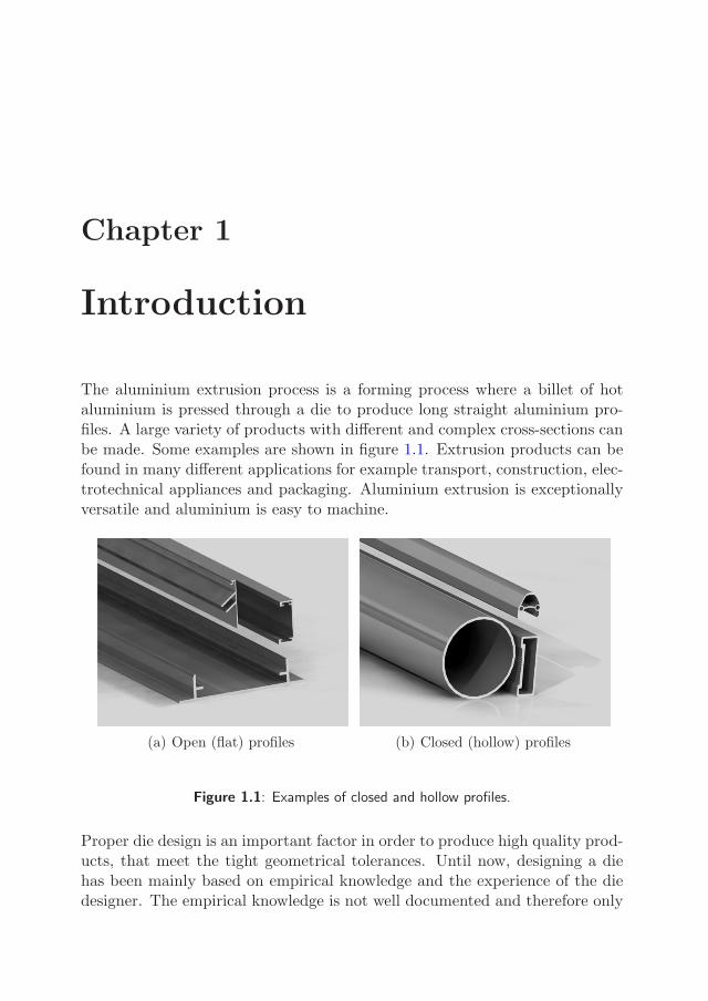
The aluminium extrusion process is a forming process where a billet of hotaluminium is pressed through a die to produce long straight aluminium pro-files. A large variety of products with different and complex cross-sections canbe made. Some examples are shown in figure 1.1. Extrusion products can befound in many different applications for example transport, construction, elec-trotechnical appliances and packaging. Aluminium extrusion is exceptionallyversatile and aluminium is easy to machine.
(a) Open (flat) profiles (b) Closed (hollow) profiles
Figure 1.1: Examples of closed and hollow profiles.
Proper die design is an important factor in order to produce high quality prod-ucts, that meet the tight geometrical tolerances. Until now, designing a diehas been mainly based on empirical knowledge and the experience of the diedesigner. The empirical knowledge is not well documented and therefore only
2
accessible by the die designer, die corrector and press operator.
In the recent years a trend toward the application of objective design rulescan be observed. Side by side with this development is the increase of the useof automated design applications, since objective design rules are required bythe design applications. Numerical methods are helpful tools to obtain quan-titative information about the process.
The finite element method (FEM) is a valuable tool to gain insight in theprocess that cannot be obtained easily otherwise. In this thesis developmentsof the FEM methods for aluminium extrusion are treated. The objective is togain more insight in the process. With this insight improved or new objectivedesign rules can be obtained.
1.1 Aluminium extrusion process
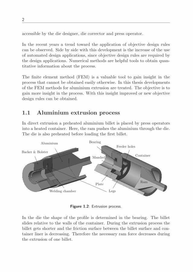
In direct extrusion a preheated aluminium billet is placed by press operatorsinto a heated container. Here, the ram pushes the aluminium through the die.The die is also preheated before loading the first billet.
Backer & Bolster
Ram
Aluminium
Mandrel
Feeder holes
Legs
Bearing
Container
Welding chamber
Plate
Figure 1.2: Extrusion process.
In the die the shape of the profile is determined in the bearing. The billetslides relative to the walls of the container. During the extrusion process thebillet gets shorter and the friction surface between the billet surface and con-tainer liner is decreasing. Therefore the necessary ram force decreases duringthe extrusion of one billet.
Introduction 3
Not all of the aluminium billet is extruded. A percentage of the compressedbillet, called the discard or butt is left at the end of the extrusion cycle. Whenthe billet is almost completely extruded, the ram and the container are re-tracted and the butt is sheared off. Then a new billet is inserted and the cycleis repeated. Since the next billet is placed after the previous, this process iscalled billet-to-billet extrusion
The profiles made using this process can be split into two groups, open andclosed profiles, as in figure 1.1. Open profiles can be made with the use of flatdies and closed profiles are made with porthole dies.
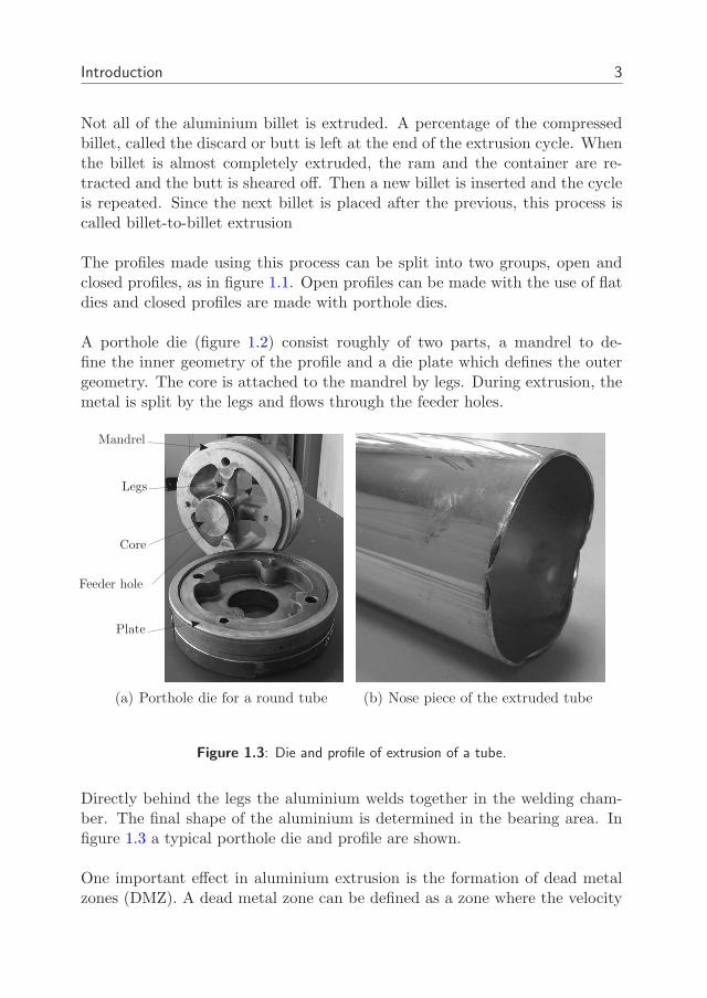
A porthole die (figure 1.2) consist roughly of two parts, a mandrel to de-fine the inner geometry of the profile and a die plate which defines the outergeometry. The core is attached to the mandrel by legs. During extrusion, themetal is split by the legs and flows through the feeder holes.
Core
Mandrel
Legs
Plate
Feeder hole
(a) Porthole die for a round tube (b) Nose piece of the extruded tube
Figure 1.3: Die and profile of extrusion of a tube.
Directly behind the legs the aluminium welds together in the welding cham-ber. The final shape of the aluminium is determined in the bearing area. Infigure 1.3 a typical porthole die and profile are shown.
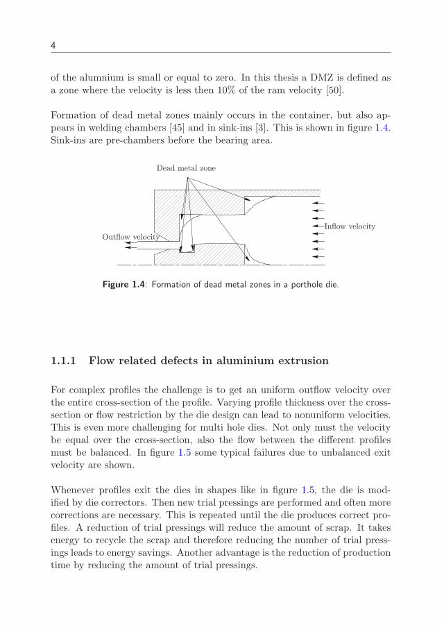
One important effect in aluminium extrusion is the formation of dead metalzones (DMZ). A dead metal zone can be defined as a zone where the velocity
4
of the alumnium is small or equal to zero. In this thesis a DMZ is defined asa zone where the velocity is less then 10% of the ram velocity [50].
Formation of dead metal zones mainly occurs in the container, but also ap-pears in welding chambers [45] and in sink-ins [3]. This is shown in figure 1.4.Sink-ins are pre-chambers before the bearing area.
Dead metal zone
Inflow velocity
Outflow velocity
Figure 1.4: Formation of dead metal zones in a porthole die.
1.1.1 Flow related defects in aluminium extrusion
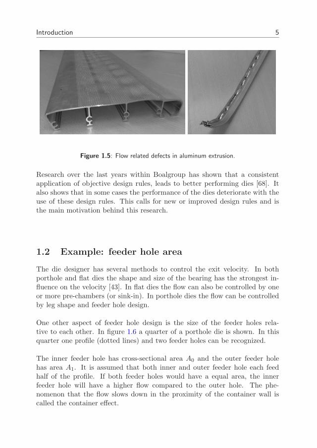
For complex profiles the challenge is to get an uniform outflow velocity overthe entire cross-section of the profile. Varying profile thickness over the cross-section or flow restriction by the die design can lead to nonuniform velocities.This is even more challenging for multi hole dies. Not only must the velocitybe equal over the cross-section, also the flow between the different profilesmust be balanced. In figure 1.5 some typical failures due to unbalanced exitvelocity are shown.
Whenever profiles exit the dies in shapes like in figure 1.5, the die is mod-ified by die correctors. Then new trial pressings are performed and often morecorrections are necessary. This is repeated until the die produces correct pro-files. A reduction of trial pressings will reduce the amount of scrap. It takesenergy to recycle the scrap and therefore reducing the number of trial press-ings leads to energy savings. Another advantage is the reduction of productiontime by reducing the amount of trial pressings.
Introduction 5
Figure 1.5: Flow related defects in aluminum extrusion.
Research over the last years within Boalgroup has shown that a consistentapplication of objective design rules, leads to better performing dies [68]. Italso shows that in some cases the performance of the dies deteriorate with theuse of these design rules. This calls for new or improved design rules and isthe main motivation behind this research.
1.2 Example: feeder hole area
The die designer has several methods to control the exit velocity. In bothporthole and flat dies the shape and size of the bearing has the strongest in-fluence on the velocity [43]. In flat dies the flow can also be controlled by oneor more pre-chambers (or sink-in). In porthole dies the flow can be controlledby leg shape and feeder hole design.
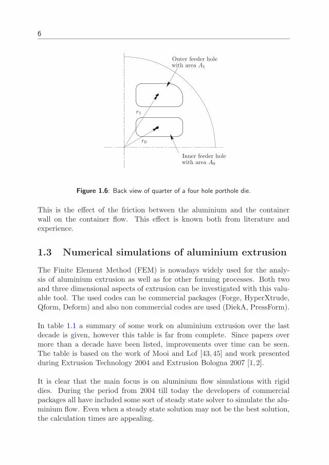
One other aspect of feeder hole design is the size of the feeder holes rela-tive to each other. In figure 1.6 a quarter of a porthole die is shown. In thisquarter one profile (dotted lines) and two feeder holes can be recognized.
The inner feeder hole has cross-sectional area A0 and the outer feeder holehas area A1. It is assumed that both inner and outer feeder hole each feedhalf of the profile. If both feeder holes would have a equal area, the innerfeeder hole will have a higher flow compared to the outer hole. The phe-nomenon that the flow slows down in the proximity of the container wall iscalled the container effect.
6
PSfrag
Inner feeder holewith area A0
Outer feeder holewith area A1
r0
r1
Figure 1.6: Back view of quarter of a four hole porthole die.
This is the effect of the friction between the aluminium and the containerwall on the container flow. This effect is known both from literature andexperience.
1.3 Numerical simulations of aluminium extrusion
The Finite Element Method (FEM) is nowadays widely used for the analy-sis of aluminium extrusion as well as for other forming processes. Both twoand three dimensional aspects of extrusion can be investigated with this valu-able tool. The used codes can be commercial packages (Forge, HyperXtrude,Qform, Deform) and also non commercial codes are used (DiekA, PressForm).
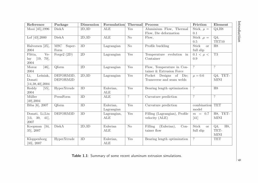
In table 1.1 a summary of some work on aluminium extrusion over the lastdecade is given, however this table is far from complete. Since papers overmore than a decade have been listed, improvements over time can be seen.The table is based on the work of Mooi and Lof [43, 45] and work presentedduring Extrusion Technology 2004 and Extrusion Bologna 2007 [1, 2].
It is clear that the main focus is on aluminium flow simulations with rigiddies. During the period from 2004 till today the developers of commercialpackages all have included some sort of steady state solver to simulate the alu-minium flow. Even when a steady state solution may not be the best solution,the calculation times are appealing.
Introduction 7
From the comparison with the overview in Mooi [45] can be recognized thatover the last ten to fifteen years the use of 3D simulations has become thestandard. Computer power and improved numerical techniques make it possi-ble to capture the start-up of the process up to steady state within reasonablesimulation times [6, 13].
Furthermore can be concluded that most commercial packages have the abilityto deal with thermo-mechanically coupled simulations. Remarkable is the lackof information in literature about thermal properties, modeled tools and otherboundary conditions. Hardly any information is available about how to modelheat transfer to the dies, ram, container and rest of the press.
In the modeling of friction large differences in the used models and valuescan be found. During the first extrusion benchmark in Zurich 2005 [54], thiswas recognized as one of the main problems to match experiments with sim-ulations. It must be remarked that in this benchmark extremely long parallelbearings were used, obviously making friction one of the important phenom-ena.
1.4 Outline of the thesis
This thesis consists of five main chapters. Chapters three, four and five arerewritten papers which have been submitted for publication elsewhere. Inchapters five and six simulations described in previous chapters are extendedwith more sophisticated elements. For the sake of readability some overlap insubject matter is present. Below an outline of the five main chapters is given.
Chapter 2: In this thesis all the simulations are performed with the FiniteElement Method. In chapter 2 an introduction in FEM methods is given.Also the used boundary conditions for Aluminium extrusion are treated.Specific attention is paid to the bearing area and streamlining the pre-processing of a complex 3D simulation.
Chapter 3: In chapter 3 a comparison is made between simulations and ex-periments of container flow. The steady state results of FEM simulationsare used as the first step in a two step procedure to create simulationresults that are compareble with the experimental results. In the sec-ond step the steady state results are post-processed to front lines. Thismethod can also be used for inverse material modeling
8
Chapter 4: The start-up of the extrusion process can feed important infor-mation to the designer. The tracking of a free surface with originalcoordinate functions to follow the flow front in an Eulerian descriptionis introduced. The results of the simulations are compared with experi-ments.
Chapter 5: Meshing complex 3D geometry with hexahedral elements fromchapter four proves to be difficult. To be able to mesh with hexahedralelements, many details are lost in the modeling. In this chapter both 2Dtriangular and 3D tetrahedral MINI elements are developed to be ableto model more detail. The tracking algorithm is implemented for theMINI elements and the simulations are repeated.
Chapter 6: To assess the reliability of the simulations, it is important tohave good experimental validation of the simulations. In chapters 3 and4 experiments are shown and in this chapter numerical results for theMINI elements are compared to these experiments. The application ofALE options in a mesh generated with the use of automatic meshers isnot straight forward. Extra attention is placed on automatic ALE optiongeneration. The trend in the numerical results is in agreement withthe experiments. Small differences can be attributed to the neglectingthermal aspects and other material data.
Intro
duction
9
Reference Package Dimension Formulation Thermal Process Friction Element
Mooi [45],1996 DiekA 2D,3D ALE Yes Aluminium Flow, ThermalFlow, Die deformation
Stick, µ =0.1
Q4,H8
Lof [43],2000 DiekA 2D,3D ALE No Flow, Stick ,µ =0.5
Q4,TET10
Halvorsen [25],2004
MSC Super-Form
3D Lagrangian No Profile buckling Stick orfull slip
H8
Flitta, Ve-lay [19, 70],2004
Forge2 (2D) 2D Lagrangian Yes Temperature evolution inContainer
0.1 < µ <
0.9T3
Moroz [46],2004
Qform 2D Lagrangian Yes Flow, Temperature in Con-tainer & Extrusion Force
? ?
Li, Lesniak,Donati[14,38,40],2004
DEFORM3D,DEFORM2D
2D,3D Lagrangian Yes Pocket Designs of Die;Transverse and seam welds
µ = 0.6 Q4, TET-MINI
Reddy [55],2004
HyperXtrude 3D Eulerian,ALE
Yes Bearing length optimization ? H8
Muller[49],2004
PressForm 3D ALE ? Curvature prediction ? ?
Biba [6], 2007 Qform 3D Eulerian,Lagrangian
Yes Curvature prediction combinationmodel
TET
Donati, Li,Liu[13, 39, 41],2007
DEFORM3D 3D Lagrangian,ALE
Yes Filling (Lagrangian), Profilevelocity (ALE)
m = 0.7[41]
H8, TET-MINI
Koopman [34,35], 2007
DiekA 2D,3D EulerianALE
No Filling (Eulerian), Con-tainer flow
Stick orfull slip
Q4, H8,TET-MINI
Kloppenborg[33], 2007
HyperXtrude 3D Eulerian,ALE
Yes Bearing length optimization ? TET
Table 1.1: Summary of some recent aluminum extrusion simulations.

10
Chapter 2
Finite element analysis of
aluminium extrusion
2.1 Introduction
The Finite Element Method (FEM) is widely accepted as an effective tool toresearch many of the extrusion flow and extrusion die properties. Over theyears the main interest is in homogenizing the outflow velocity. Other thanthat topic also weld seam quality prediction, prediction of temperature distri-bution and prediction of die wear and lifetime is performed.
The finite element method can also be used to optimize the extrusion pro-file design. Aluminium is widely used in construction. A better quantificationof the structural properties through FEM simulations can lead to significantmaterial reduction. An example of FEM analysis on profiles can be foundin [47]. In that research profiles for window framing are optimized for a mini-mum of thermal conductivity to obtain higher insulation values.
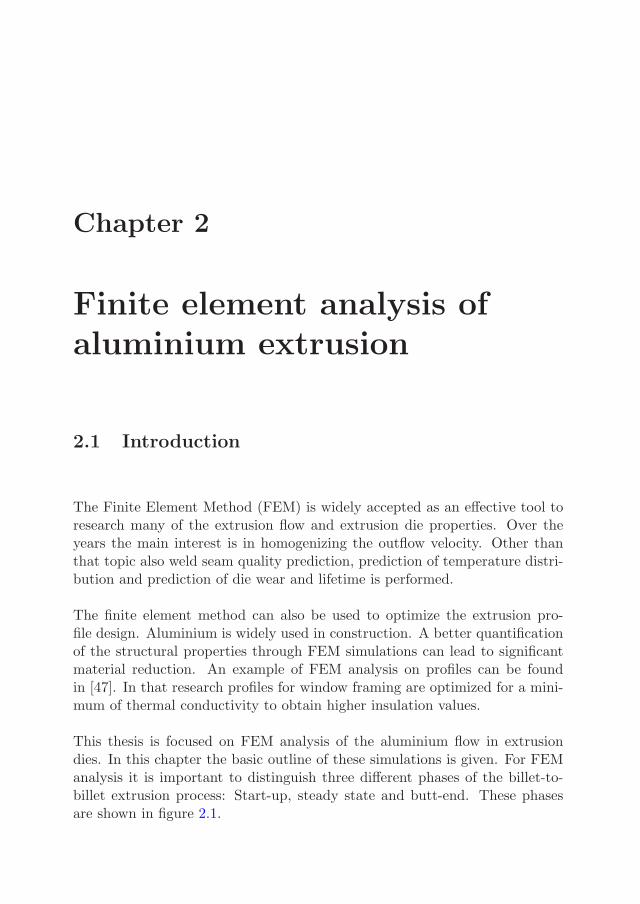
This thesis is focused on FEM analysis of the aluminium flow in extrusiondies. In this chapter the basic outline of these simulations is given. For FEManalysis it is important to distinguish three different phases of the billet-to-billet extrusion process: Start-up, steady state and butt-end. These phasesare shown in figure 2.1.
12
start-up
The first phase is the start-up of the process, see figure 2.1(a). In this phasethe die cavity is filled with aluminium.When the second or next billet is loaded,the die is already filled with aluminium and the process is restarted. In thisthesis, start-up is defined as the die filling and first meters of the profile.
This first length of profile is commonly used by the die correctors to eval-uate the adjustments to be made on the die to get a homogeneous outflowvelocity. This first length is called the nose piece. In chapter 4 an algorithmis treated that is able to capture this part of the process in a FEM analysis.
steady state
After start-up, the process can be regarded as a steady-state process. There isa steady inflow of aluminium into the deformation zone and a steady outflowof aluminium in the form of the profile. The uniform and constant inflow onlyholds when the ram is far away from the deformation zone. This should betaken into account when modeling a steady state flow. Since the inflow of
(a) Start-up (b) Steady state (c) Butt end
Figure 2.1: Three process parts in billet to billet extrusion. The begin at the top row (I)and end (I) of each part is at the bottom row.
aluminium is constant, only a part of the billet needs to be modeled. At theinflow side of the modeled part a constant inflow velocity, equal to the ramspeed, is applied. This is shown in figure 2.1(b). The length of the billet to bemodeled Lbil is chosen between one and one and a half of the billet diameterDbil. The constant inflow velocity should develop into a plug flow that usuallyappears inside the container away from the die. In our experience the chosenbillet length is sufficient to allow for this, before entering the deformation zone.
At the outflow side many conditions can be applied. Default is chosen fora free outflow condition. This condition allows for the material to flow out
Finite element analysis of aluminium extrusion 13
with non homogeneous velocity. The velocity profile tells something aboutthe effectiveness of the die-design. Another condition can be constraints thatinvoke the velocity to be constant over the cross-section. This resembles aprofile that is clamped in a puller and therefore forced to be straight. Alsothickening or thinning because of velocity effects can be described with thiscondition.
butt-end
In the final phase the ram gets close to the die. Here it starts to interferewith the deformation zone. This marks the end of the second phase becausethe steady state conditions are no longer valid. Usually the next phase is notsimulated, since it is only a small part of the process. The last centimeters ofthe billet are not extruded, since it contains the build up contamination andoxidation of the complete billet [36]. This last part, the butt-end, is shearedoff at the die face. The next billet is placed and the loop is started over.
In this thesis only the start-up and steady state simulations are shown. Steadystate simulations are convenient since they are much less time consuming thanthe transient (start-up and butt-end) simulations. However start-up gives thedesigner very valuable information about the effectiveness of the die. Theactual nose piece can be derived and used for evaluation of the die. In thenext sections the framework for both start-up and steady state simulationsare described.
2.2 Different FEM formulations
Aluminium extrusion can be modeled with different types of FEM. In thissection some types of FEM formulations are discussed and assessed on theirsuitability for modeling aluminium extrusion. The different phases in billet-to-billet extrusion raise their own demands. In the start-up phase the formulationshould be able to describe large deformations and free surfaces. In the steadystate phase, the ability to model a free surface is not required.
2.2.1 Lagrangian formulation
In forming processes a Lagrangian formulation is often used. The mesh isfixed to the material and deforms accordingly. In this formulation the frameof reference is equal to the initial geometry (Total Lagrangian) or equal tothe deformed geometry and moving with the material (Updated Lagrangian).
14
Since the mesh is fixed to the material, free surfaces are accurately followed.A drawback of the updated Lagrangian formulation is that when the materialundergoes large deformations, the mesh can become severely distorted. Dis-torted elements will lead to less accurate results or when elements flip insideout lead to a premature end of the simulation.
To accommodate these problems to be able to model aluminium extrusionwith an updated Lagrangian formulation, remeshing techniques have been de-veloped. Remeshing is widely used for simulation of forming processes. Themost important issues in remeshing are the creation of a new mesh and theremapping of the state variables from the old mesh onto the new mesh.
The main drawback of using an Updated Lagrangian formulation with remesh-ing for the simulation of aluminium extrusion is the time involved in remeshingand remapping.
2.2.2 Eulerian formulation
In an Eulerian formulation material flows through the mesh. The mesh is keptat the initial location. This will avoid all of the problems involving the meshdistortions. However since free surfaces are almost never equal to the elementedges, tracking the free surface is not as straight forward as in Lagrangian for-mulations. In chapter 4 some procedures for tracking free surfaces are treated.Where in Lagrangian formulations the history dependent state variables arereadily known, in Eulerian formulations they have to be convected throughthe mesh every step.
2.2.3 ALE formulation
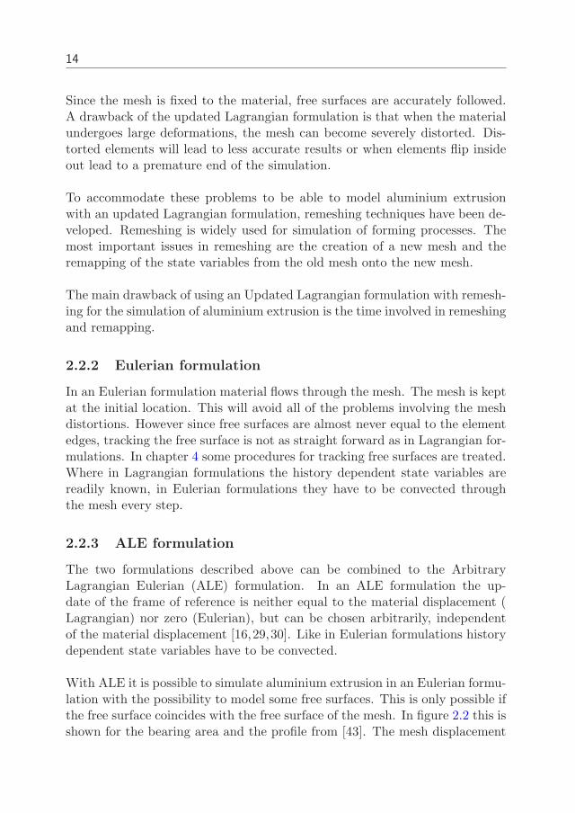
The two formulations described above can be combined to the ArbitraryLagrangian Eulerian (ALE) formulation. In an ALE formulation the up-date of the frame of reference is neither equal to the material displacement (Lagrangian) nor zero (Eulerian), but can be chosen arbitrarily, independentof the material displacement [16,29,30]. Like in Eulerian formulations historydependent state variables have to be convected.
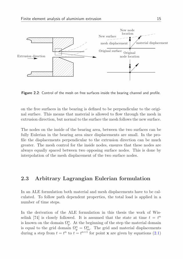
With ALE it is possible to simulate aluminium extrusion in an Eulerian formu-lation with the possibility to model some free surfaces. This is only possible ifthe free surface coincides with the free surface of the mesh. In figure 2.2 this isshown for the bearing area and the profile from [43]. The mesh displacement
Finite element analysis of aluminium extrusion 15
Originalnode location
New surface
New nodelocation
material displacementmesh displacement
Original surface
Extrusion direction
Figure 2.2: Control of the mesh on free surfaces inside the bearing channel and profile.
on the free surfaces in the bearing is defined to be perpendicular to the origi-nal surface. This means that material is allowed to flow through the mesh inextrusion direction, but normal to the surface the mesh follows the new surface.
The nodes on the inside of the bearing area, between the two surfaces can befully Eulerian in the bearing area since displacements are small. In the pro-file the displacements perpendicular to the extrusion direction can be muchgreater. The mesh control for the inside nodes, ensures that these nodes arealways equally spaced between two opposing surface nodes. This is done byinterpolation of the mesh displacement of the two surface nodes.
2.3 Arbitrary Lagrangian Eulerian formulation
In an ALE formulation both material and mesh displacements have to be cal-culated. To follow path dependent properties, the total load is applied in anumber of time steps.
In the derivation of the ALE formulation in this thesis the work of Wis-selink [74] is closely followed. It is assumed that the state at time t = tn
is known on the domain Ωng . At the beginning of the step the material domain
is equal to the grid domain Ωng = Ωn
m. The grid and material displacementsduring a step from t = tn to t = tn+1 for point x are given by equations (2.1)
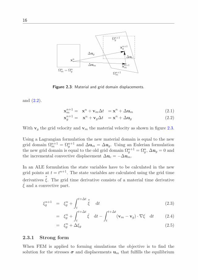
16
Ωnm = Ωn
gΩn+1
m
Ωn+1g
xn+1g
xn+1m
xn
∆um
∆ug∆uc
Figure 2.3: Material and grid domain displacements.
and (2.2).
xn+1m = xn + vm∆t = xn + ∆um (2.1)
xn+1g = xn + vg∆t = xn + ∆ug (2.2)
With vg the grid velocity and vm the material velocity as shown in figure 2.3.
Using a Lagrangian formulation the new material domain is equal to the newgrid domain Ωn+1
m = Ωn+1g and ∆um = ∆ug. Using an Eulerian formulation
the new grid domain is equal to the old grid domain Ωn+1g = Ωn
g , ∆ug = 0 andthe incremental convective displacement ∆uc = −∆um.
In an ALE formulation the state variables have to be calculated in the newgrid points at t = tn+1. The state variables are calculated using the grid time
derivatives∗ξ. The grid time derivative consists of a material time derivative
ξ and a convective part.
ξn+1g = ξn
g +
∫ t+∆t
t
∗ξ dt (2.3)
= ξng +
∫ t+∆t
t
ξ dt −∫ t+∆t
t
(vm − vg) · ∇ξ dt (2.4)
= ξng + ∆ξg (2.5)
2.3.1 Strong form
When FEM is applied to forming simulations the objective is to find thesolution for the stresses σ and displacements um that fulfills the equilibrium
Finite element analysis of aluminium extrusion 17
equations and boundary conditions at tn+1. The surface is split into a part Γu
where the displacements are prescribed: un+10 , and a part Γt where the forces
are prescribed: tn+1.
σn+1 · ∇ = 0 in Ωn+1
g
u = un+10 on Γu
σn+1 · n = tn+1 on Γt
(2.6)
with n the outward normal on the boundary. Furthermore inflow conditionsare set for state variables and displacements at the boundary Γf where materialflows into the domain.
u = uf on Γf
ξ = ξf on Γf(2.7)
2.3.2 Weak form
In FEM the equilibrium equations are only weakly enforced. The constitutiverelations are the material rate of the stress-strain relations. Therefore the rateof the weak form is used. In appendix A the rate of the weak form for ALE isderived. Here only the result is given:
∫
Ωw∇ : [−Lg · σ + σ − (vm − vg) · ∇σ + σtr(Lg)] dΩ =
∫
Γw · t dΓ −
∫
Γw · [(vm − vg) · ∇σ]n dΓ (2.8)
With w the weighing function, Lg the gradient of the grid velocity and theintegration is over the spatial coordinates. For an Updated Lagrangian for-mulation, since vm = vg, this degenerates to:
∫
Ωw∇ : [−L · σ + σ + σtr(L)] dΩ =
∫
Γw · t dΓ (2.9)
With L the gradient of the material velocity.
2.3.3 Coupled and semi-coupled ALE
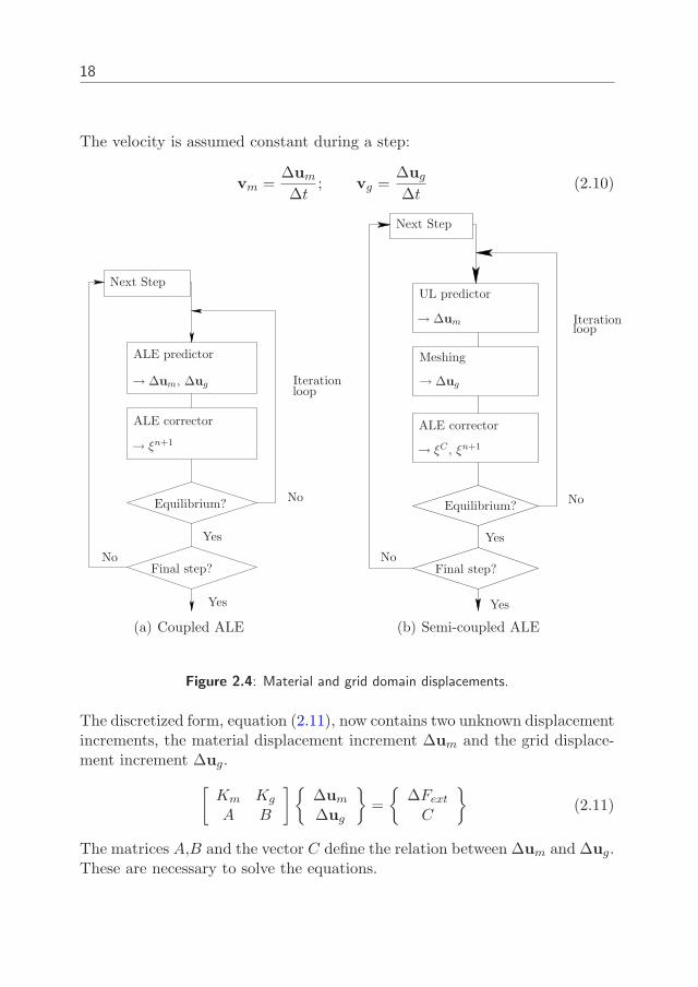
For a coupled ALE formulation equation (2.8) is discretized. In a coupled for-mulation both material and convective terms are solved simultaneously andtherefore a coupled formulation yields the best possible solution of the ALEproblem. In figure 2.4(a) the solution strategy for a coupled ALE formulationis shown. The complete derivation can be found in Appendix A.
18
The velocity is assumed constant during a step:
vm =∆um
∆t; vg =
∆ug
∆t(2.10)
ALE predictor
→ ∆um, ∆ug
ALE corrector
→ ξn+1
Next Step
Equilibrium?No
No
Yes
Yes
Final step?
Iterationloop
(a) Coupled ALE
ALE corrector
→ ξC , ξn+1
Next Step
Equilibrium?No
No
Yes
Yes
Final step?
UL predictor
→ ∆um
Meshing
→ ∆ug
Iterationloop
(b) Semi-coupled ALE
Figure 2.4: Material and grid domain displacements.
The discretized form, equation (2.11), now contains two unknown displacementincrements, the material displacement increment ∆um and the grid displace-ment increment ∆ug.
[
Km Kg
A B
]
∆um
∆ug
=
∆Fext
C
(2.11)
The matrices A,B and the vector C define the relation between ∆um and ∆ug.These are necessary to solve the equations.
Finite element analysis of aluminium extrusion 19
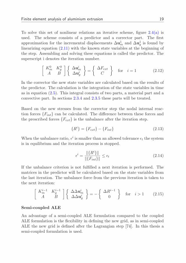
To solve this set of nonlinear relations an iterative scheme, figure 2.4(a) isused. The scheme consists of a predictor and a corrector part. The firstapproximation for the incremental displacements ∆u1
m and ∆u1g is found by
linearizing equation (2.11) with the known state variables at the beginning ofthe step. Assembling and solving these equations is called the predictor. Thesuperscript i denotes the iteration number.
[
K0m K0
g
A B
]
∆uim
∆uig
=
∆Fext
C
for i = 1 (2.12)
In the corrector the new state variables are calculated based on the results ofthe predictor. The calculation is the integration of the state variables in timeas in equation (2.5). This integral consists of two parts, a material part and aconvective part. In sections 2.3.4 and 2.3.5 these parts will be treated.
Based on the new stresses from the corrector step the nodal internal reac-tion forces Fint can be calculated. The difference between these forces andthe prescribed forces Fext is the unbalance after the iteration step.
Ri = Fext − Fint (2.13)
When the unbalance ratio, εi is smaller than an allowed tolerance εt the systemis in equilibrium and the iteration process is stopped.
εi =‖Ri‖‖Fint‖
≤ εt (2.14)
If the unbalance criterion is not fulfilled a next iteration is performed. Thematrices in the predictor will be calculated based on the state variables fromthe last iteration. The unbalance force from the previous iteration is taken tothe next iteration:
[
Ki−1m Ki−1
g
A B
]
∆∆uim
∆∆uig
= −
∆Ri−1
0
for i > 1 (2.15)
Semi-coupled ALE
An advantage of a semi-coupled ALE formulation compared to the coupledALE formulation is the flexibility in defining the new grid, as in semi-coupledALE the new grid is defined after the Lagrangian step [74]. In this thesis asemi-coupled formulation is used.
20
In figure 2.4(b) the scheme for a semi-coupled ALE formulation is shown.With respect to the coupled ALE scheme, the ALE predictor is replaced by aUL predictor by setting ∆ug = ∆um and discretizing equation (2.9). After theUL predictor a meshing step is performed to calculate the grid displacementincrement ∆ug.
In the corrector step first the convective increment of the state variables ξC iscalculated based on the values at the beginning of the step.
ξC(xn+1g ) = ξ0(xn
m − ∆uc) (2.16)
The problem in calculation of ξC(xn+1g ) is that ξ0 is only known in the inte-
gration points and the field is discontinuous. In section 2.3.5 this problem istreated in more detail.
Next the material increment is calculated by integration of the material ratein time:
ξn+1 = ξC +
∫ t+∆t
t
ξdt (2.17)
With these new state variables the unbalance is calculated. By comparisonwith the unbalance criterion is checked whether the new state variables are inequilibrium.
The advantage of the semi coupled ALE method is the flexibility in mesh-ing compared to the coupled ALE. Also the equilibrium is fulfilled at the endof a step. The semi-coupled formulation is less efficient than the decoupled,since the convection and meshing are performed each iteration step.
In the next paragraphs is shown how the material and convective incrementresp. are calculated.
2.3.4 Material increment
The constitutive equations describe the relation between the stresses and thestrains. In this section the constitutive elasto-viscoplastic model is presented,which has been implemented into the FEM code.
The strain is decomposed in an elastic and a viscoplastic part. The equa-tion is given in incremental form, obtained by integrating the constitutiverelations in rate form. The integration is over a time increment [tn, tn+1] with
Finite element analysis of aluminium extrusion 21
an implicit Euler backward scheme.
∆ε = ∆εe + ∆ε
vp (2.18)
Hooke’s law relates the Cauchy stress tensor σ to the elastic strain tensor. TheCauchy stress tensor relates to the material frame of reference. In appendixA the stress tensor for a co-rotational frame of reference is given. In equation(2.19) E is a fourth order tensor based on the Young’s modulus E and thepoisson ration ν.
∆σ = E : (∆ε − ∆εvp) (2.19)
The viscoplastic strain increment is assumed to be in the direction of thedeviatoric stress. The plastic multiplier ∆λ is used to scale the viscoplasticstrain rate.
∆εvp = ∆λsn+1 (2.20)
with s the deviatoric stress tensor defined as σ = s − pI and the hydrostaticpressure as p = −tr(σ). The limit function describes the rate dependentbehavior of the material in the plastic domain.
gn+1(σn+1, κn+1, κn+1) = σn+1 − σy(κn+1, κn+1, T ) (2.21)
The Von Mises criterion is used to define the effective stress σ.
σ =
√
3
2s : s (2.22)
The flow stress σy is a function of the state variables, κ and κ, representingthe equivalent plastic strain and equivalent plastic strain rate respectively.
κn+1 = κn +
√
2
3∆εvp : ∆εvp (2.23)
κn+1 =
√
23∆εvp : ∆εvp
∆t(2.24)
From equation (2.20) and (2.24) the relation between the plastic multiplierand the incremental equivalent plastic strain can be derived.
∆κn+1 =
√
2
3∆εvp : ∆εvp =
√
2
3∆λsn+1 : ∆λsn+1
∆λ
√
2
3sn+1 : sn+1 =
2
3∆λ
√
3
2sn+1 : sn+1 =
2
3∆λσn+1 (2.25)
22
The material can be in two states. In the elastic state the plastic multiplier iszero and the limit function is smaller then or equal to zero. In the viscoplasticstate the plastic multiplier is greater than zero and the limit function is equalto zero. This is captured by the Kuhn-Tucker loading-unloading conditions.
∆λ ≥ 0, ∆λgn+1 = 0, gn+1 ≤ 0 (2.26)
In the correction step the new total strain increments are calculated. Basedon these strains a new elastic trial stress is calculated. If the trial stress fulfillsthe Kuhn-Tucker condition this is assumed the actual stress and the materialis elastic.
If the Kuhn-Tucker relations are not satisfied by the elastic trial stress, thematerial is in the plastic state. The stresses are then calculated by enforcingthat the limit function gn+1 = 0. Looking at the deviatoric stresses and strainsonly, equation (2.19) can be written as:
sn+1 = sn + 2G(∆e − ∆λsn+1) (2.27)
and for the limit function in equation (2.21):
gn+1 =
√
3
2sn+1 : sn+1 − σy(κn+1, κn+1, T ) = 0 (2.28)
With G the shear modulus and ∆e the deviatoric part of the total strain in-crement.
Sometimes an explicit equation for the plastic multiplier ∆λ can be found,but in most cases an iterative approach is necessary to determine ∆λ. Forthis purpose a Newton-Raphson method can be used, but calculation of thederivative of g can be expensive to compute. In this work a secant method isused, which requires only the evaluation of g [43].
To obtain objective integration the derivation of Lof [44] is closely followed.Lof chooses to use a corotational formulation. The initial deviatoric stresssn+1 is replaced by sn+1:
sn+1 = Rsn+1RT (2.29)
Where R follows from the polar decomposition of the incremental deformationgradient F.
Finite element analysis of aluminium extrusion 23
Material model
The constitutive behavior of aluminium is represented by the limit functionequation (2.21) and a relation for the flow stress. In this work the simulationsare performed using the Sellars-Tegart law [43].
σy = smarcsinh(
( κ
Aexp( Q
RT
))1
m
)
(2.30)
The relation is given between the flow stress σy, κ and T . sm and m are strainsensitivity parameters. These are assumed to be constant. Q is the apparentactivation energy of the deformation process during plastic flow. R is the uni-versal gas constant, T the absolute temperature and A is a factor, dependingexplicitly on the Magnesium and Silicium content in the aluminium matrix.Because of the high temperatures during extrusion, the strain hardening canbe neglected [31].
In table 2.1 the material properties for AA6063 alloy are summarized. Inthis work simulations are performed using these properties, unless mentionedotherwise.
Table 2.1: Material parameters for AA6063 alloy [43].
Symbol value
Elastic properties E [MPa] 40000(T=823K) ν [-] 0.4995
Plastic properties sm [MPa] 25m [-] 5.4
A [1/s] 6 · 109
Q [J/mol] 1.4 · 105
R [J/molK] 8.314
The reason for ν = 0.4995 is to reduce the amount of elastic compression atthe start of the simulations. With an value that makes the aluminium nearlyincompressible, the simulation reaches the staedy state much faster.
2.3.5 Convective increment
For semi-coupled ALE the convective increment has to be calculated everyiteration. This convective increment can be written as a convection or inter-polation problem or a mix of those two. Since the velocity is assumed constant
24
during a step the convective increment can be written as:
∆ξC =
∫ t+∆t
t
−vc · ∇ξdt ≈ −∆uc · ∇ξ (2.31)
The main difficulty is to calculate the gradient ∇ξ. Stresses and strains areonly evaluated in the integration points and are discontinuous over the elementboundaries. This means that the gradient ∇ξ cannot be determined locally,since this would ignore the jump over the element boundaries. Therefore in-formation of neighboring elements is necessary to construct a global gradient.
The history dependent state variables, like equivalent plastic strain and stress,are known in the integration points of the elements. These state variables haveto be remapped from the old location of the integration points to the new lo-cations. Nodal values, like displacements, are not necessary for the FEManalysis, but can be useful for the analysis of the results.
Courant number
For the calculation of the convective increment the Courant number is used.In this thesis the Courant number is defined as the difference in local coordi-nates between the old and the new integration point locations, divided by thecharacteristic element length l. This depends on the element type of choice.
Cr =1
nrip
nrip∑
ip=1
|∆rip|l
, Cz = . . . (2.32)
The three courant numbers Cr, Cz and Ch are calculated for the differentdirections in every integration point. The element average is given in equation(2.33). The total courant number is written as:
C =√
C2r + C2
z + C2h (2.33)
2.3.6 Convection scheme
Many methods for the calculation of ∆ξC have been proposed. Two mainmethods can be distinguished. The finite element method used by [29,74] andthe finite volume method used by [28].
Usage of the finite element method for the convective increment in an ALE
Finite element analysis of aluminium extrusion 25
method has the main advantage that the Lagrangian step is also performedwith the finite element method, which facilitates the implementation of themethod. One of the Taylor-Galerkin methods [15] is the WLGS scheme pro-posed by [29]. This scheme requires a continuous distribution of the statevariable across the element boundaries. Creating this continuous field tendsto smooth the gradients between the elements.
The discontinuous Galerkin method, which is a generalization of the finitevolume method, [21,23,37,53] allows for discontinuities across element bound-aries. In [23] a second order Discontinuous Galerkin scheme is presented.The 2D convection tests yield far better accuracy than standard discontinu-ous Galerkin methods and the WLGS scheme. The scheme is also attractivein an ALE method since it uses the existing mesh of the Lagrangian step.Development and implementation of 3D versions of this scheme would be aninteresting topic.
In this research the focus is mainly on the convection of nodal values. Sincenodal values are already continuous, it can be expected the WLGS schemeyields more accurate results than for integration point values. In chapter 4the accuracy of the WLGS scheme for nodal values is shown.
Weighted local and global smoothing
The new integration point values are calculated by the use of the weightedlocal and global smoothing (WLGS) scheme described in [29, 71, 74]. In thisthesis a summary of the WLGS scheme presented in Wisselink [74] is given.
The WLGS is an interpolation approach, which uses an intermediate step tocreate a smoothed continuous field from the integration point values. Thereare two steps to be distinguished in the WLGS scheme:
1. At the end of each step a continuous field is constructed from the inte-gration point data values. The same field used at the beginning of thenext step
a First the integration point values are extrapolated to the nodes,with a local smoothing factor
b From the extrapolated values the nodal averages are calculated
c These averaged values are interpolated back to the integration points
26
2. The integration point values are calculated in the new integration pointslocations using the continuous field
a First the Courant numbers are calculated
b Based on the Courant numbers the global smoothing factor is cal-culated
c The integration point values in the new integration point locationsare calculated using the global smoothing factor and the continuousfields
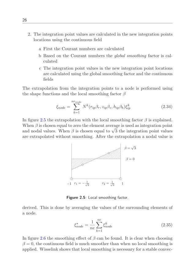
The extrapolation from the integration points to a node is performed usingthe shape functions and the local smoothing factor β
ξnode =
nrnode∑
k=1
Nk(ripβr, zipβz, hipβh)ξkip (2.34)
In figure 2.5 the extrapolation with the local smoothing factor β is explained.When β is chosen equal to zero the element average is used as integration pointand nodal values. When β is chosen equal to
√3 the integration point values
are extrapolated without smoothing. After the extrapolation a nodal value is
−1 1
β = 0
β =√
3
r1 = − 1√3
r2 = 1√3
Figure 2.5: Local smoothing factor.
derived. This is done by averaging the values of the surrounding elements ofa node.
ξ∗node =1
ne
ne∑
k=1
ξknode (2.35)
In figure 2.6 the smoothing effect of β can be found. It is clear when choosingβ = 0, the continuous field is much smoother than when no local smoothing isapplied. Wisselink shows that local smoothing is necessary for a stable convec-
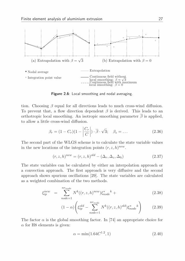
Finite element analysis of aluminium extrusion 27
(a) Extrapolation with β =√
3 (b) Extrapolation with β = 0
Nodal average
Integration point value Continuous field withoutlocal smoothing: β =
√3
Continuous field with maximumlocal smoothing: β = 0
Extrapolation
Figure 2.6: Local smoothing and nodal averaging.
tion. Choosing β equal for all directions leads to much cross-wind diffusion.To prevent that, a flow direction dependent β is derived. This leads to anorthotropic local smoothing. An isotropic smoothing parameter β is applied,to allow a little cross-wind diffusion.
βr = (1 − Cr)(1 −∣
∣
∣
∣
Cr
C
∣
∣
∣
∣
) · β ·√
3; βz = . . . (2.36)
The second part of the WLGS scheme is to calculate the state variable valuesin the new locations of the integration points (r, z, h)new.
(r, z, h)new = (r, z, h)old − (∆r, ∆z, ∆h) (2.37)
The state variables can be calculated by either an interpolation approach ora convection approach. The first approach is very diffusive and the secondapproach shows spurious oscillations [29]. The state variables are calculatedas a weighted combination of the two methods.
ξnewip =
nrnode∑
node=1
Nk((r, z, h)new)ξ∗nodek + (2.38)
(1 − α)
(
ξoldip −
nrnode∑
node=1
Nk((r, z, h)old)ξ∗nodek
)
(2.39)
The factor α is the global smoothing factor. In [74] an appropriate choice forα for H8 elements is given:
α = min(1.64C1.2, 1) (2.40)
28
Convective increment for nodal values
The total displacements are nodal values. For some elements pressures arenodal values as well instead of integration point values. The convection ofnodal values is treated slightly different compared to integration point values.This is discussed in chapter 4
2.4 Modeling aluminium extrusion
In this section specific aspects of FEM analysis of aluminium extrusion aretreated. First is described how a 3D FEM model for extrusion is created. Inthis pre-processing some simplifications are made to the die design to be moretime efficient in both pre-processing and solving the equations.
2.4.1 Pre-processing
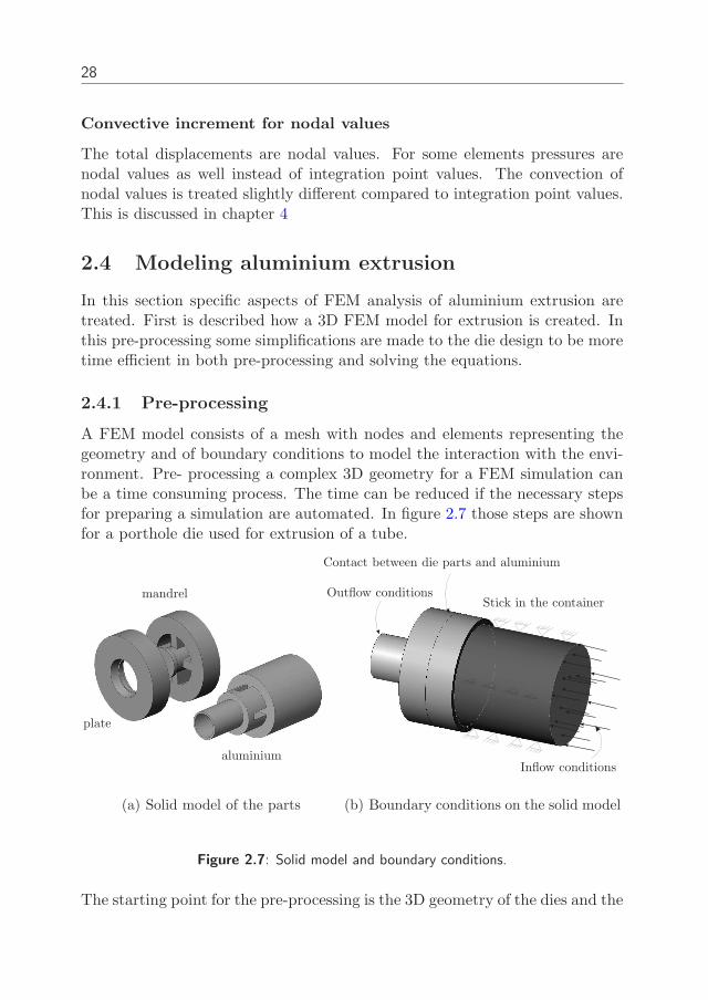
A FEM model consists of a mesh with nodes and elements representing thegeometry and of boundary conditions to model the interaction with the envi-ronment. Pre- processing a complex 3D geometry for a FEM simulation canbe a time consuming process. The time can be reduced if the necessary stepsfor preparing a simulation are automated. In figure 2.7 those steps are shownfor a porthole die used for extrusion of a tube.
aluminium
mandrel
plate
(a) Solid model of the parts
Inflow conditions
Outflow conditionsStick in the container
Contact between die parts and aluminium
(b) Boundary conditions on the solid model
Figure 2.7: Solid model and boundary conditions.
The starting point for the pre-processing is the 3D geometry of the dies and the
Finite element analysis of aluminium extrusion 29
aluminium. In this research SolidWorks is used for modeling the 3D geometry.The aluminium inside the dies is taken as a negative of the die cavity. Partsof the profile and billet are added to that negative.
Before the mesh is created the boundary conditions are applied to the solidmodel as in figure 2.7(b). All the boundary conditions are applied to thesurface areas or surface lines. The most important boundary conditions are:
Inflow of aluminium At the inflow surface of the billet the material velocityis prescribed uniform and equal to the ram speed. The outer edge of theinflow surface touches the container wall. Here a choice has to be madewhether to have a sticking condition here or a slip condition with materialvelocity. In this thesis, the outer edge has the material inflow velocityand a free slip condition with the container. This condition ensuresthat the whole inflow surface has a uniform velocity and the inflow isdetermined exactly. This is convenient for setting the ram speed andtesting the volume conservation properties.
Outflow of aluminium At the outflow surface of the billet the material ve-locity can be constrained to be uniform or otherwise constrained. Inthe simulations in this thesis, no special conditions are applied at theoutflow, unless mentioned otherwise.
Contact between aluminium and the container Contact between alumin-ium and container is always modeled as stick. In other words, the mate-rial displacement is equal to zero in all directions. That this assumptionis allowed has been shown in [43].
Contact between aluminium and die The contact between aluminiumand die parts is also modeled as stick, except for the bearing area. Herespecial conditions are applied. These conditions are treated in the nextparagraphs.
Definition of bearing area To transfer the special conditions in the bearingarea from the solid model to the FEM model, the bearing area has to bedefined. The boundary conditions on the bearing area are special andregular pre-processors don’t have the ability to apply these conditions.Therefore this conditions are applied in a next phase. In this phasedummy forces are placed on the nodes on the bearing surface. In thenext phase these dummy forces are used as markers and not transferredas force.
30
Definition of bearing corner The boundary on the bearing corner also needsspecial attention. The definition of these conditions is treated in the nextparagraph. On the bearing corner also a marker is placed.
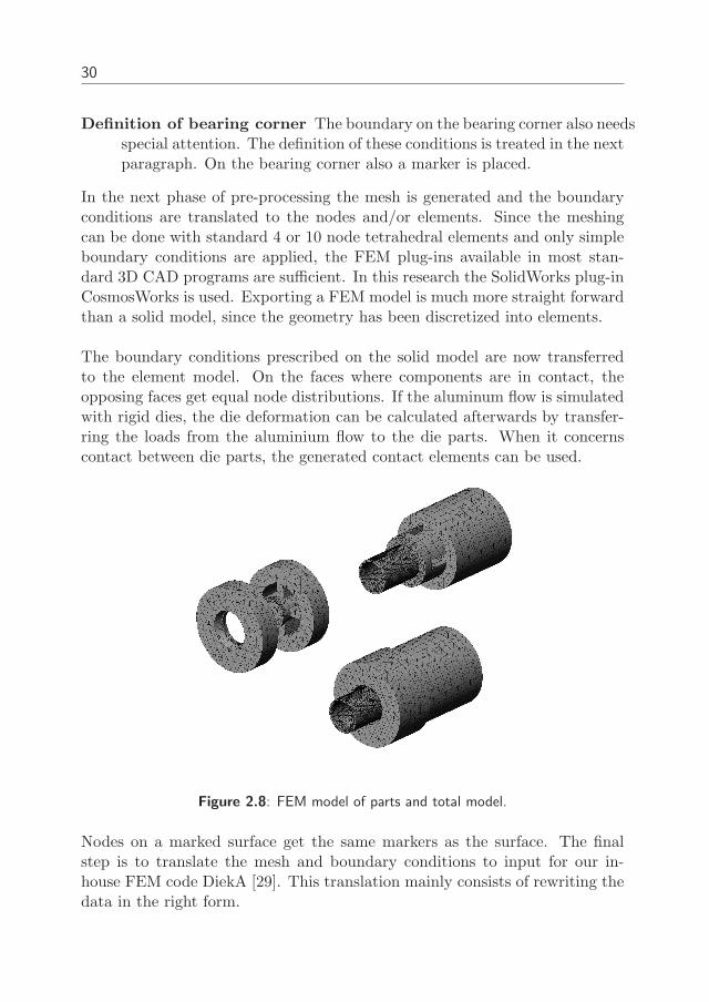
In the next phase of pre-processing the mesh is generated and the boundaryconditions are translated to the nodes and/or elements. Since the meshingcan be done with standard 4 or 10 node tetrahedral elements and only simpleboundary conditions are applied, the FEM plug-ins available in most stan-dard 3D CAD programs are sufficient. In this research the SolidWorks plug-inCosmosWorks is used. Exporting a FEM model is much more straight forwardthan a solid model, since the geometry has been discretized into elements.
The boundary conditions prescribed on the solid model are now transferredto the element model. On the faces where components are in contact, theopposing faces get equal node distributions. If the aluminum flow is simulatedwith rigid dies, the die deformation can be calculated afterwards by transfer-ring the loads from the aluminium flow to the die parts. When it concernscontact between die parts, the generated contact elements can be used.
Figure 2.8: FEM model of parts and total model.
Nodes on a marked surface get the same markers as the surface. The finalstep is to translate the mesh and boundary conditions to input for our in-house FEM code DiekA [29]. This translation mainly consists of rewriting thedata in the right form.
Finite element analysis of aluminium extrusion 31
3D CAD
Die 1.partDie n.part
Total.assemb FEM-plugin FEMmod.db
Alu.part
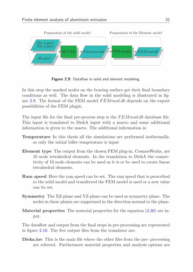
Preparation of the solid model Preparation of the Element model
Figure 2.9: Dataflow in solid and element modeling.
In this step the marked nodes on the bearing surface get their final boundaryconditions as well. The data flow in the solid modeling is illustrated in fig-ure 2.9. The format of the FEM model FEMmod.db depends on the exportpossibilities of the FEM plugin.
The input file for the final pre-process step is the FEMmod.db database file.This input is translated to DiekA input with a macro and some additionalinformation is given to the macro. The additional information is:
Temperature In this thesis all the simulations are performed isothermally,so only the initial billet temperature is input
Element type The output from the chosen FEM plug-in, CosmosWorks, are10 node tetrahedral elements. In the translation to DiekA the connec-tivity of 10 node elements can be used as it is or be used to create lineartetrahedral elements.
Ram speed Here the ram speed can be set. The ram speed that is prescribedto the solid model and transferred the FEM model is used or a new valuecan be set.
Symmetry The XZ-plane and YZ-plane can be used as symmetry plane. Thenodes in these planes are suppressed in the direction normal to the plane.
Material properties The material properties for the equation (2.30) are in-put.
The dataflow and output from the final steps in pre-processing are representedin figure 2.10. The five output files from the translator are:
Dieka.inv This is the main file where the other files from the pre- processingare referred. Furthermore material properties and analysis options are
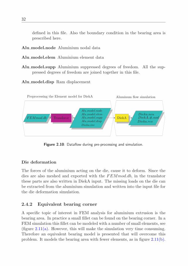
32
defined in this file. Also the boundary condition in the bearing area isprescribed here.
Alu model.node Aluminium nodal data
Alu model.elem Aluminium element data
Alu model.supp Aluminium suppressed degrees of freedom. All the sup-pressed degrees of freedom are joined together in this file.
Alu model.disp Ram displacement
Preprocessing the Element model for DiekA Aluminum flow simulation
FEMmod.db Translator
Alu model.node
Alu model.elemAlu model.supp
Alu model.disp
Dieka.inv
DiekADieka.neuDiekA #.nodDieka.res
Figure 2.10: Dataflow during pre-processing and simulation.
Die deformation
The forces of the aluminium acting on the die, cause it to deform. Since thedies are also meshed and exported with the FEMmod.db, in the translatorthese parts are also written in DiekA input. The missing loads on the die canbe extracted from the aluminium simulation and written into the input file forthe die deformation simulation.
2.4.2 Equivalent bearing corner
A specific topic of interest in FEM analysis for aluminium extrusion is thebearing area. In practice a small fillet can be found on the bearing corner. In aFEM simulation this fillet can be modeled with a number of small elements, see(figure 2.11(a). However, this will make the simulation very time consuming.Therefore an equivalent bearing model is presented that will overcome thisproblem. It models the bearing area with fewer elements, as in figure 2.11(b).
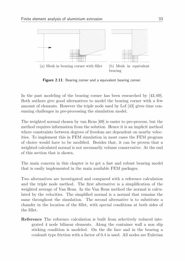
Finite element analysis of aluminium extrusion 33
(a) Mesh in bearing corner with fillet (b) Mesh in equivalentbearing
Figure 2.11: Bearing corner and a equivalent bearing corner.
In the past modeling of the bearing corner has been researched by [43, 69].Both authors give good alternatives to model the bearing corner with a fewamount of elements. However the triple node used by Lof [43] gives time con-suming challenges in pre-processing the simulation model.
The weighted normal chosen by van Rens [69] is easier to pre-process, but themethod requires information from the solution. Hence it is an implicit methodwhere constraints between degrees of freedom are dependent on nearby veloc-ities. To implement this in FEM simulation in most cases the FEM programof choice would have to be modified. Besides that, it can be proven that aweighted calculated normal is not necessarily volume conservative. At the endof this section that is shown.
The main concern in this chapter is to get a fast and robust bearing modelthat is easily implemented in the main available FEM packages.
Two alternatives are investigated and compared with a reference calculationand the triple node method. The first alternative is a simplification of theweighted average of Van Rens. In the Van Rens method the normal is calcu-lated by the velocities. The simplified normal is a normal that remains thesame throughout the simulation. The second alternative is to substitute achamfer in the location of the fillet, with special conditions at both sides ofthe fillet.
Reference The reference calculation is built from selectively reduced inte-grated 4 node bilinear elements. Along the container wall a non slipsticking condition is modeled. On the die face and in the bearing acoulomb type friction with a factor of 0.4 is used. All nodes are Eulerian
34
except for the nodes on the contact surface, they are ALE with onlynode movement perpendicular to the surface.
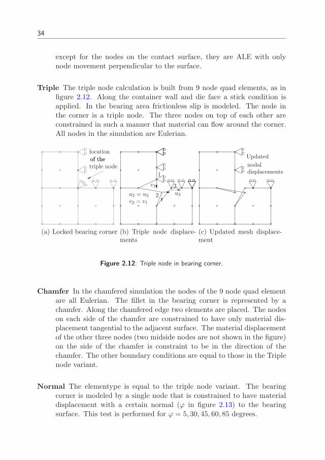
Triple The triple node calculation is built from 9 node quad elements, as infigure 2.12. Along the container wall and die face a stick condition isapplied. In the bearing area frictionless slip is modeled. The node inthe corner is a triple node. The three nodes on top of each other areconstrained in such a manner that material can flow around the corner.All nodes in the simulation are Eulerian.
location
of theof thetriple node
(a) Locked bearing corner
1
2
3v1
u3
v2 = v1
u2 = u3
(b) Triple node displace-ments
Updated
nodaldisplacements
(c) Updated mesh displace-ment
Figure 2.12: Triple node in bearing corner.
Chamfer In the chamfered simulation the nodes of the 9 node quad elementare all Eulerian. The fillet in the bearing corner is represented by achamfer. Along the chamfered edge two elements are placed. The nodeson each side of the chamfer are constrained to have only material dis-placement tangential to the adjacent surface. The material displacementof the other three nodes (two midside nodes are not shown in the figure)on the side of the chamfer is constraint to be in the direction of thechamfer. The other boundary conditions are equal to those in the Triplenode variant.
Normal The elementype is equal to the triple node variant. The bearingcorner is modeled by a single node that is constrained to have materialdisplacement with a certain normal (ϕ in figure 2.13) to the bearingsurface. This test is performed for ϕ = 5, 30, 45, 60, 85 degrees.
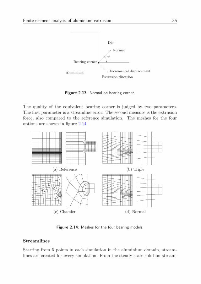
Finite element analysis of aluminium extrusion 35
Extrusion directionAluminium
Die
ϕ
Bearing corner
Normal
Incremental displacement
Figure 2.13: Normal on bearing corner.
The quality of the equivalent bearing corner is judged by two parameters.The first parameter is a streamline error. The second measure is the extrusionforce, also compared to the reference simulation. The meshes for the fouroptions are shown in figure 2.14.
(a) Reference (b) Triple
(c) Chamfer (d) Normal
Figure 2.14: Meshes for the four bearing models.
Streamlines
Starting from 5 points in each simulation in the aluminium domain, stream-lines are created for every simulation. From the steady state solution stream-
36
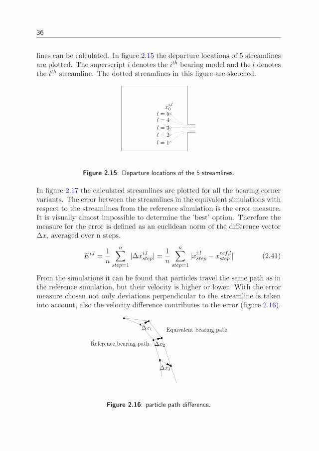
lines can be calculated. In figure 2.15 the departure locations of 5 streamlinesare plotted. The superscript i denotes the ith bearing model and the l denotesthe lth streamline. The dotted streamlines in this figure are sketched.
l = 1
l = 2
l = 3
l = 4l = 5
xi,l0
Figure 2.15: Departure locations of the 5 streamlines.
In figure 2.17 the calculated streamlines are plotted for all the bearing cornervariants. The error between the streamlines in the equivalent simulations withrespect to the streamlines from the reference simulation is the error measure.It is visually almost impossible to determine the ’best’ option. Therefore themeasure for the error is defined as an euclidean norm of the difference vector∆x, averaged over n steps.
Ei,l =1
n
n∑
step=1
|∆xi,lstep| =
1
n
n∑
step=1
|xi,lstep − x
ref,lstep | (2.41)
From the simulations it can be found that particles travel the same path as inthe reference simulation, but their velocity is higher or lower. With the errormeasure chosen not only deviations perpendicular to the streamline is takeninto account, also the velocity difference contributes to the error (figure 2.16).
∆x1
∆x2
∆x3
Equivalent bearing path
Reference bearing path
Figure 2.16: particle path difference.
Finite element analysis of aluminium extrusion 37
20
30
40
ReferenceTripleChamferNormal 5
x
y31
90 100 110
(a) ER=9
20
30
40
ReferenceNormal 30Normal 45Normal 60Normal 85
xy
90 100 110
(b) ER=9
30
150
ReferenceTripleChamferNormal 5
x
y
29
31
90 100 110
(c) ER=45
30ReferenceNormal 30Normal 45Normal 60Normal 85
x
y
29
31
90 100 110
(d) ER=45
Figure 2.17: Streamlines.
In figure 2.18 the error is plotted. At one axis the 5 streamlines are expandedat the other axis the 8 bearing node variants.
Observing the results for extrusion ratio 9, the triple node out performs allother variants. This effect is less severe for an extrusion ratio of 45. From
38
figure 2.17 can be seen that the error of streamline 3 is mainly a velocityerror.
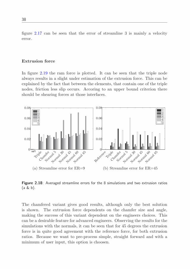
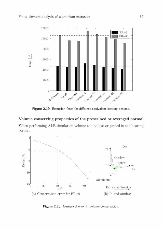
Extrusion force
In figure 2.19 the ram force is plotted. It can be seen that the triple nodealways results in a slight under estimation of the extrusion force. This can beexplained by the fact that between the elements, that contain one of the triplenodes, friction less slip occurs. Accoring to an upper bound criterion thereshould be shearing forces at those interfaces.
ref10
0.02
0.04
0.06
0.0812345
Triple
Cha
mfer
Normal
5
Normal
30
Normal
45
Normal
60
Normal
85
(a) Streamline error for ER=9
0
0.02
0.04
0.06
0.0812345
Referen
ce
Triple
Cha
mfer
Normal
5
Normal
30
Normal
45
Normal
60
Normal
85
(b) Streamline error for ER=45
Figure 2.18: Averaged streamline errors for the 8 simulations and two extrusion ratios(a & b).
The chamfered variant gives good results, although only the best solutionis shown. The extrusion force dependents on the chamfer size and angle,making the success of this variant dependent on the engineers choices. Thiscan be a desirable feature for advanced engineers. Observing the results for thesimulations with the normals, it can be seen that for 45 degrees the extrusionforce is in quite good agreement with the reference force, for both extrusionratios. Because we want to pre-process simple, straight forward and with aminimum of user input, this option is choosen.
Finite element analysis of aluminium extrusion 39
0
ER=9ER=45
2000
4000
6000
8000
10000
12000
Referenc
e
Triple
Chamfer
Normal
5
Normal
30
Normal
45
Normal
60
Normal
85
For
ce[
Nm
m
]
Figure 2.19: Extrusion force for different equivalent bearing options.
Volume conserving properties of the prescribed or averaged normal
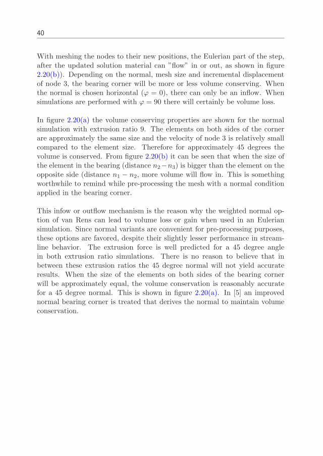
When performing ALE simulation volume can be lost or gained in the bearingcorner.
−15
−5
0
0
5
20 40 60 80ϕ[ ]
Error V
[%]
-10
(a) Conservation error for ER=9
n1
n2
n3
Extrusion direction
Aluminium
Die
Outflow
Inflow
ϕ
(b) In and outflow
Figure 2.20: Numerical error in volume conservation.
40
With meshing the nodes to their new positions, the Eulerian part of the step,after the updated solution material can ”flow” in or out, as shown in figure2.20(b)). Depending on the normal, mesh size and incremental displacementof node 3, the bearing corner will be more or less volume conserving. Whenthe normal is chosen horizontal (ϕ = 0), there can only be an inflow. Whensimulations are performed with ϕ = 90 there will certainly be volume loss.
In figure 2.20(a) the volume conserving properties are shown for the normalsimulation with extrusion ratio 9. The elements on both sides of the cornerare approximately the same size and the velocity of node 3 is relatively smallcompared to the element size. Therefore for approximately 45 degrees thevolume is conserved. From figure 2.20(b) it can be seen that when the size ofthe element in the bearing (distance n2−n3) is bigger than the element on theopposite side (distance n1 − n2, more volume will flow in. This is somethingworthwhile to remind while pre-processing the mesh with a normal conditionapplied in the bearing corner.
This infow or outflow mechanism is the reason why the weighted normal op-tion of van Rens can lead to volume loss or gain when used in an Euleriansimulation. Since normal variants are convenient for pre-processing purposes,these options are favored, despite their slightly lesser performance in stream-line behavior. The extrusion force is well predicted for a 45 degree anglein both extrusion ratio simulations. There is no reason to believe that inbetween these extrusion ratios the 45 degree normal will not yield accurateresults. When the size of the elements on both sides of the bearing cornerwill be approximately equal, the volume conservation is reasonably accuratefor a 45 degree normal. This is shown in figure 2.20(a). In [5] an improvednormal bearing corner is treated that derives the normal to maintain volumeconservation.
Chapter 3
Front line tracking in a steady
state flow
3.1 Introduction
In this chapter aluminium flow inside the container is studied. Extrusion ex-periments are performed at Boalgroup to visualize the flow inside the containerduring extrusion.
These experiments are compared with simulations. In section 3.3 a proce-dure is treated to obtain comparable numerical results. The procedure is firstdemonstrated on a Newtonian viscous flow.
The numerical results are fitted to the experiments by adapting the materialparameters. To yield accurate flow results in a simulation, accurate materialproperties are necessary. In this chapter it is shown that the procedure canbe used for an inverse determination of material parameters. Determining thematerial properties is usually done by compression or torsion tests [43]. How-ever these tests do not give results under extrusion conditions of high pressureand shear strain. Comparison of aluminium flow between experiments andsimulations [65], [66] inside a container, can lead to better material properties,among other simulation parameters.
3.2 Experiments
Extrusion experiments are performed with aluminium billets prepared as infigure 3.1. First a cylindrical billet of 210 mm long is cut into slices of 15
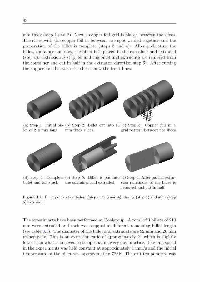
42
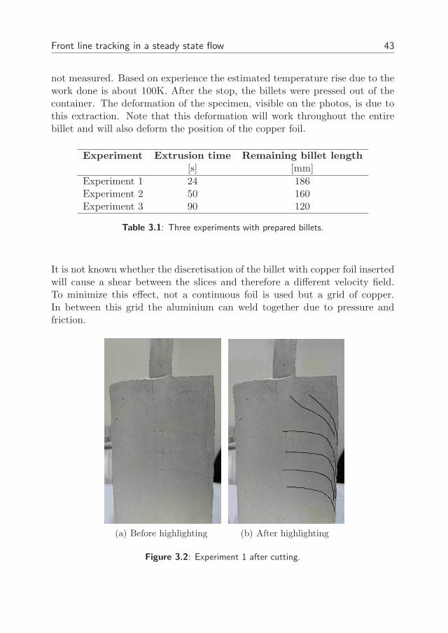
mm thick (step 1 and 2). Next a copper foil grid is placed between the slices.The slices,with the copper foil in between, are spot welded together and thepreparation of the billet is complete (steps 3 and 4). After preheating thebillet, container and dies, the billet it is placed in the container and extruded(step 5). Extrusion is stopped and the billet and extrudate are removed fromthe container and cut in half in the extrusion direction step 6). After cuttingthe copper foils between the slices show the front lines.
(a) Step 1: Initial bil-let of 210 mm long
(b) Step 2: Billet cut into 15mm thick slices
(c) Step 3: Copper foil in agrid pattern between the slices
(d) Step 4: Completebillet and foil stack
(e) Step 5: Billet is put intothe container and extruded
(f) Step 6: After partial extru-sion remainder of the billet isremoved and cut in half
Figure 3.1: Billet preparation before (steps 1,2, 3 and 4), during (step 5) and after (step6) extrusion.
The experiments have been performed at Boalgroup. A total of 3 billets of 210mm were extruded and each was stopped at different remaining billet length(see table 3.1). The diameter of the billet and extrudate are 92 mm and 20 mmrespectively. This is an extrusion ratio of approximately 21 which is slightlylower than what is believed to be optimal in every day practice. The ram speedin the experiments was held constant at approximately 1 mm/s and the initialtemperature of the billet was approximately 723K. The exit temperature was
Front line tracking in a steady state flow 43
not measured. Based on experience the estimated temperature rise due to thework done is about 100K. After the stop, the billets were pressed out of thecontainer. The deformation of the specimen, visible on the photos, is due tothis extraction. Note that this deformation will work throughout the entirebillet and will also deform the position of the copper foil.
Experiment Extrusion time Remaining billet length
[s] [mm]
Experiment 1 24 186Experiment 2 50 160Experiment 3 90 120
Table 3.1: Three experiments with prepared billets.
It is not known whether the discretisation of the billet with copper foil insertedwill cause a shear between the slices and therefore a different velocity field.To minimize this effect, not a continuous foil is used but a grid of copper.In between this grid the aluminium can weld together due to pressure andfriction.
(a) Before highlighting (b) After highlighting
Figure 3.2: Experiment 1 after cutting.
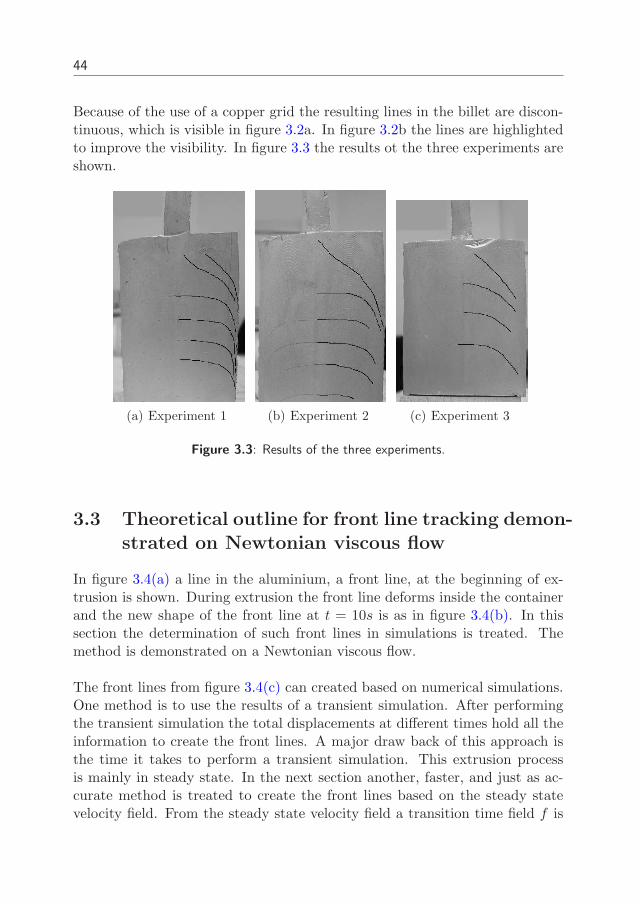
44
Because of the use of a copper grid the resulting lines in the billet are discon-tinuous, which is visible in figure 3.2a. In figure 3.2b the lines are highlightedto improve the visibility. In figure 3.3 the results ot the three experiments areshown.
(a) Experiment 1 (b) Experiment 2 (c) Experiment 3
Figure 3.3: Results of the three experiments.
3.3 Theoretical outline for front line tracking demon-
strated on Newtonian viscous flow
In figure 3.4(a) a line in the aluminium, a front line, at the beginning of ex-trusion is shown. During extrusion the front line deforms inside the containerand the new shape of the front line at t = 10s is as in figure 3.4(b). In thissection the determination of such front lines in simulations is treated. Themethod is demonstrated on a Newtonian viscous flow.
The front lines from figure 3.4(c) can created based on numerical simulations.One method is to use the results of a transient simulation. After performingthe transient simulation the total displacements at different times hold all theinformation to create the front lines. A major draw back of this approach isthe time it takes to perform a transient simulation. This extrusion processis mainly in steady state. In the next section another, faster, and just as ac-curate method is treated to create the front lines based on the steady statevelocity field. From the steady state velocity field a transition time field f is
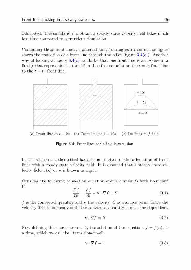
Front line tracking in a steady state flow 45
calculated. The simulation to obtain a steady state velocity field takes muchless time compared to a transient simulation.
Combining these front lines at different times during extrusion in one figureshows the transition of a front line through the billet (figure 3.4(c)). Anotherway of looking at figure 3.4(c) would be that one front line is an isoline in afield f that represents the transition time from a point on the t = t0 front lineto the t = tn front line.
(a) Front line at t = 0s (b) Front line at t = 10s
t = 0
t = 5s
t = 10s
(c) Iso-lines in f -field
Figure 3.4: Front lines and f-field in extrusion.
In this section the theoretical background is given of the calculation of frontlines with a steady state velocity field. It is assumed that a steady state ve-locity field v(x) or v is known as input.
Consider the following convection equation over a domain Ω with boundaryΓ.
Df
Dt=
∂f
∂t+ v · ∇f = S (3.1)
f is the convected quantity and v the velocity. S is a source term. Since thevelocity field is in steady state the convected quantity is not time dependent.
v · ∇f = S (3.2)
Now defining the source term as 1, the solution of the equation, f = f(x), isa time, which we call the ”transition-time”.
v · ∇f = 1 (3.3)
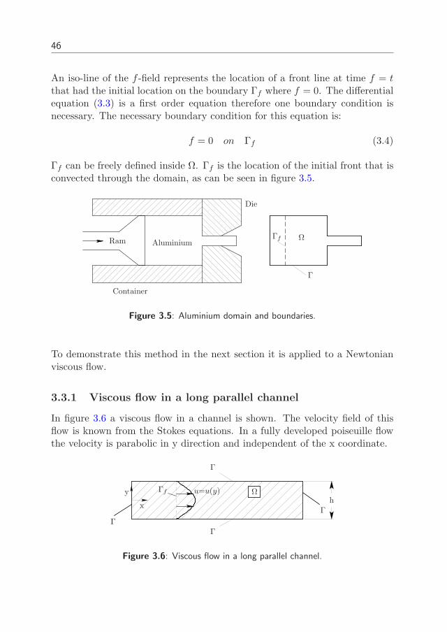
46
An iso-line of the f -field represents the location of a front line at time f = t
that had the initial location on the boundary Γf where f = 0. The differentialequation (3.3) is a first order equation therefore one boundary condition isnecessary. The necessary boundary condition for this equation is:
f = 0 on Γf (3.4)
Γf can be freely defined inside Ω. Γf is the location of the initial front that isconvected through the domain, as can be seen in figure 3.5.
Aluminium
Die
Ram ΩΓf
Γ
Container
Figure 3.5: Aluminium domain and boundaries.
To demonstrate this method in the next section it is applied to a Newtonianviscous flow.
3.3.1 Viscous flow in a long parallel channel
In figure 3.6 a viscous flow in a channel is shown. The velocity field of thisflow is known from the Stokes equations. In a fully developed poiseuille flowthe velocity is parabolic in y direction and independent of the x coordinate.
xh
y Γf
Γ
Γ
u=u(y) Ω
Γ
Γ
Figure 3.6: Viscous flow in a long parallel channel.
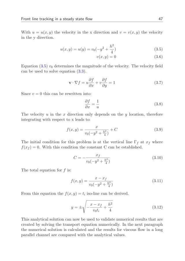
Front line tracking in a steady state flow 47
With u = u(x, y) the velocity in the x direction and v = v(x, y) the velocityin the y direction.
u(x, y) = u(y) = v0(−y2 +h2
4) (3.5)
v(x, y) = 0 (3.6)
Equation (3.5) v0 determines the magnitude of the velocity. The velocity fieldcan be used to solve equation (3.3).
v · ∇f = u∂f
∂x+ v
∂f
∂y= 1 (3.7)
Since v = 0 this can be rewritten into:
∂f
∂x=
1
u(3.8)
The velocity u in the x direction only depends on the y location, thereforeintegrating with respect to x leads to:
f(x, y) =x
v0(−y2 + h2
4 )+ C (3.9)
The initial condition for this problem is at the vertical line Γf at xf wheref(xf ) = 0. With this condition the constant C can be established.
C = − xf
v0(−y2 + h2
4 )(3.10)
The total equation for f is:
f(x, y) =x − xf
v0(−y2 + h2
4 )(3.11)
From this equation the f(x, y) = ti iso-line can be derived.
y = ±√
−x − xf
v0ti+
h2
4(3.12)
This analytical solution can now be used to validate numerical results that arecreated by solving the transport equation numerically. In the next paragraphthe numerical solution is calculated and the results for viscous flow in a longparallel channel are compared with the analytical values.
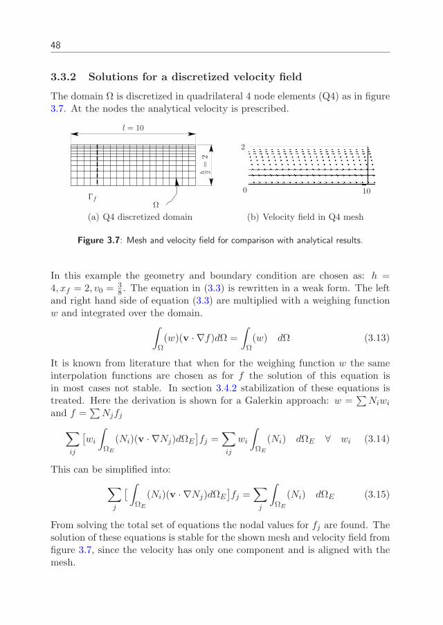
48
3.3.2 Solutions for a discretized velocity field
The domain Ω is discretized in quadrilateral 4 node elements (Q4) as in figure3.7. At the nodes the analytical velocity is prescribed.
Γf
Ωh 2
=2
l = 10
(a) Q4 discretized domain
2
100
(b) Velocity field in Q4 mesh
Figure 3.7: Mesh and velocity field for comparison with analytical results.
In this example the geometry and boundary condition are chosen as: h =4, xf = 2, v0 = 3
8 . The equation in (3.3) is rewritten in a weak form. The leftand right hand side of equation (3.3) are multiplied with a weighing functionw and integrated over the domain.
∫
Ω(w)(v · ∇f)dΩ =
∫
Ω(w) dΩ (3.13)
It is known from literature that when for the weighing function w the sameinterpolation functions are chosen as for f the solution of this equation isin most cases not stable. In section 3.4.2 stabilization of these equations istreated. Here the derivation is shown for a Galerkin approach: w =
∑
Niwi
and f =∑
Njfj
∑
ij
[
wi
∫
ΩE
(Ni)(v · ∇Nj)dΩE
]
fj =∑
ij
wi
∫
ΩE
(Ni) dΩE ∀ wi (3.14)
This can be simplified into:
∑
j
[
∫
ΩE
(Ni)(v · ∇Nj)dΩE
]
fj =∑
j
∫
ΩE
(Ni) dΩE (3.15)
From solving the total set of equations the nodal values for fj are found. Thesolution of these equations is stable for the shown mesh and velocity field fromfigure 3.7, since the velocity has only one component and is aligned with themesh.
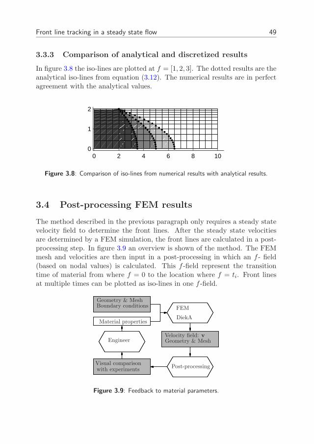
Front line tracking in a steady state flow 49
3.3.3 Comparison of analytical and discretized results
In figure 3.8 the iso-lines are plotted at f = [1, 2, 3]. The dotted results are theanalytical iso-lines from equation (3.12). The numerical results are in perfectagreement with the analytical values.
0 2 4 6 8 100
1
2
Figure 3.8: Comparison of iso-lines from numerical results with analytical results.
3.4 Post-processing FEM results
The method described in the previous paragraph only requires a steady statevelocity field to determine the front lines. After the steady state velocitiesare determined by a FEM simulation, the front lines are calculated in a post-processing step. In figure 3.9 an overview is shown of the method. The FEMmesh and velocities are then input in a post-processing in which an f - field(based on nodal values) is calculated. This f -field represent the transitiontime of material from where f = 0 to the location where f = ti. Front linesat multiple times can be plotted as iso-lines in one f -field.
Engineer Geometry & Mesh
Geometry & MeshBoundary conditions FEM
DiekA
Velocity field: v
Post-processingVisual comparisonwith experiments
Material properties
Figure 3.9: Feedback to material parameters.
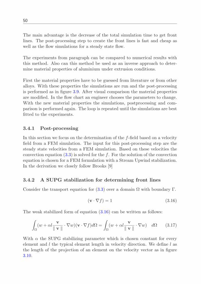
50
The main advantage is the decrease of the total simulation time to get frontlines. The post-processing step to create the front lines is fast and cheap aswell as the flow simulations for a steady state flow.
The experiments from paragraph can be compared to numerical results withthis method. Also can this method be used as an inverse approach to deter-mine material properties of aluminium under extrusion conditions.
First the material properties have to be guessed from literature or from otheralloys. With these properties the simulations are run and the post-processingis performed as in figure 3.9. After visual comparison the material propertiesare modified. In the flow chart an engineer chooses the parameters to change.With the new material properties the simulations, postprocessing and com-parison is performed again. The loop is repeated until the simulations are bestfitted to the experiments.
3.4.1 Post-processing
In this section we focus on the determination of the f -field based on a velocityfield from a FEM simulation. The input for this post-processing step are thesteady state velocities from a FEM simulation. Based on these velocities theconvection equation (3.3) is solved for the f . For the solution of the convectionequation is chosen for a FEM formulation with a Stream Upwind stabilization.In the derivation we closely follow Brooks [9]
3.4.2 A SUPG stabilization for determining front lines
Consider the transport equation for (3.3) over a domain Ω with boundary Γ.
(v · ∇f) = 1 (3.16)
The weak stabilized form of equation (3.16) can be written as follows:
∫
Ω(w + αl
v
‖ v ‖ · ∇w)(v · ∇f)dΩ =
∫
Ω(w + αl
v
‖ v ‖ · ∇w) dΩ (3.17)
With α the SUPG stabilizing parameter which is chosen constant for everyelement and l the typical element length in velocity direction. We define l asthe length of the projection of an element on the velocity vector as in figure3.10.
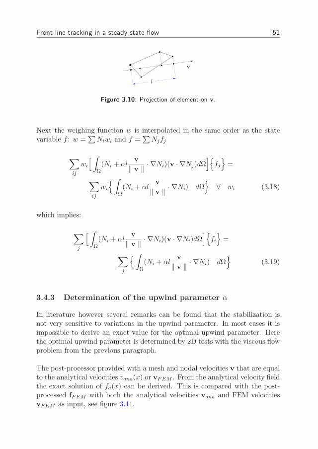
Front line tracking in a steady state flow 51
v
l
Figure 3.10: Projection of element on v.
Next the weighing function w is interpolated in the same order as the statevariable f : w =
∑
Niwi and f =∑
Njfj
∑
ij
wi
[
∫
Ω(Ni + αl
v
‖ v ‖ · ∇Ni)(v · ∇Nj)dΩ]
fj
=
∑
ij
wi
∫
Ω(Ni + αl
v
‖ v ‖ · ∇Ni) dΩ
∀ wi (3.18)
which implies:
∑
j
[
∫
Ω(Ni + αl
v
‖ v ‖ · ∇Ni)(v · ∇Ni)dΩ]
fi
=
∑
j
∫
Ω(Ni + αl
v
‖ v ‖ · ∇Ni) dΩ
(3.19)
3.4.3 Determination of the upwind parameter α
In literature however several remarks can be found that the stabilization isnot very sensitive to variations in the upwind parameter. In most cases it isimpossible to derive an exact value for the optimal upwind parameter. Herethe optimal upwind parameter is determined by 2D tests with the viscous flowproblem from the previous paragraph.
The post-processor provided with a mesh and nodal velocities v that are equalto the analytical velocities vana(x) or vFEM . From the analytical velocity fieldthe exact solution of fa(x) can be derived. This is compared with the post-processed fFEM with both the analytical velocities vana and FEM velocitiesvFEM as input, see figure 3.11.
52
Ω
Γ
Γ
Γf
Γf
FEM
Analytical
vFEM
vana(x)
vana
post-processing fFEM
analytical fa(x)
fFEM = ti
fa(x) = ti
Determination of velocity field
Determination of f field
Figure 3.11: Accuracy test of SUPG algorithm.
In figure 3.12 results of the post-processor are shown. The analytical velocityfield from equation (3.6) is used as input in the post-processor to create theresults in the left column. As mentioned before this solution is stable evenwithout upwind stabilization. From equation (3.19) we can derive that forthis specific case there is no need for stabilization and it even has no contri-bution. This effect is apparent in the left column of figure 3.12. Here thepost-processor gives exact results for any upwind parameter.
The calculation of the f -field in right column is based on velocities from FEMcalculations vFEM . The inflow condition in the FEM calculation is an uniforminflow velocity on the left side which will develop to a poiseuille flow. Thisvelocity field will give instabilities for α = 0 as can be seen in the right columnof figure 3.12. Choosing an upwind parameter in the range between 0.1 and 1will give good results. Higher values will diffuse the field excessively.
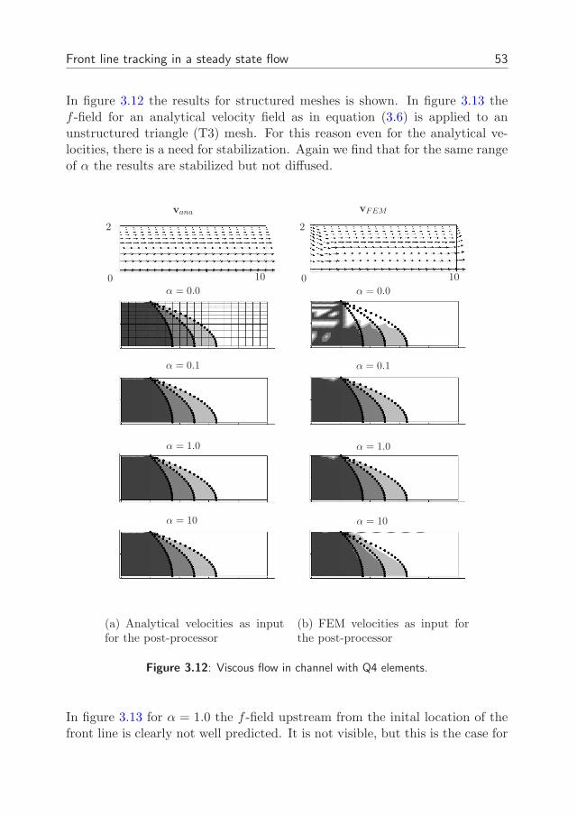
Front line tracking in a steady state flow 53
In figure 3.12 the results for structured meshes is shown. In figure 3.13 thef -field for an analytical velocity field as in equation (3.6) is applied to anunstructured triangle (T3) mesh. For this reason even for the analytical ve-locities, there is a need for stabilization. Again we find that for the same rangeof α the results are stabilized but not diffused.
129
vana
α = 0.0
α = 0.1
α = 1.0
α = 10
10
2
0
(a) Analytical velocities as inputfor the post-processor
vFEM
α = 0.0
α = 0.1
α = 1.0
α = 10
10
2
0
(b) FEM velocities as input forthe post-processor
Figure 3.12: Viscous flow in channel with Q4 elements.
In figure 3.13 for α = 1.0 the f -field upstream from the inital location of thefront line is clearly not well predicted. It is not visible, but this is the case for
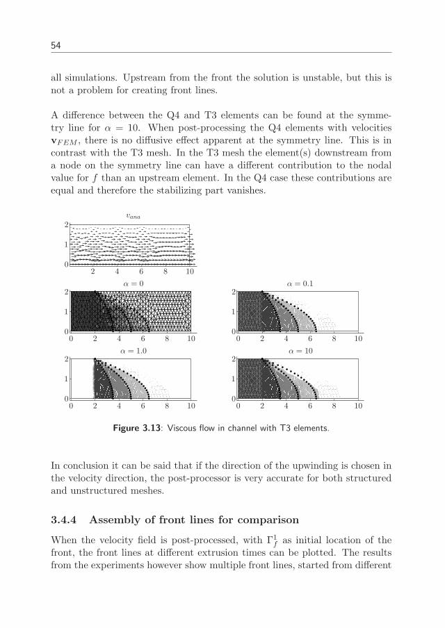
54
all simulations. Upstream from the front the solution is unstable, but this isnot a problem for creating front lines.
A difference between the Q4 and T3 elements can be found at the symme-try line for α = 10. When post-processing the Q4 elements with velocitiesvFEM , there is no diffusive effect apparent at the symmetry line. This is incontrast with the T3 mesh. In the T3 mesh the element(s) downstream froma node on the symmetry line can have a different contribution to the nodalvalue for f than an upstream element. In the Q4 case these contributions areequal and therefore the stabilizing part vanishes.
0
00
00
00
00
1
11
11
2
2
2
2
2
2
2
2
2
2
4
44
44
6
66
66
8
88
88
10
1010
1010
133
vana
α = 10
α = 0 α = 0.1
α = 1.0
Figure 3.13: Viscous flow in channel with T3 elements.
In conclusion it can be said that if the direction of the upwinding is chosen inthe velocity direction, the post-processor is very accurate for both structuredand unstructured meshes.
3.4.4 Assembly of front lines for comparison
When the velocity field is post-processed, with Γ1f as initial location of the
front, the front lines at different extrusion times can be plotted. The resultsfrom the experiments however show multiple front lines, started from different
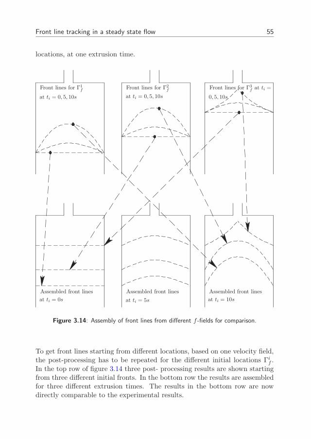
Front line tracking in a steady state flow 55
locations, at one extrusion time.
Front lines for Γ1f Front lines for Γ2
f Front lines for Γ3f at ti =
Assembled front lines Assembled front lines Assembled front lines
at ti = 0, 5, 10s at ti = 0, 5, 10s 0, 5, 10s
at ti = 0s at ti = 5s at ti = 10s
Figure 3.14: Assembly of front lines from different f -fields for comparison.
To get front lines starting from different locations, based on one velocity field,the post-processing has to be repeated for the different initial locations Γi
f .In the top row of figure 3.14 three post- processing results are shown startingfrom three different initial fronts. In the bottom row the results are assembledfor three different extrusion times. The results in the bottom row are nowdirectly comparable to the experimental results.
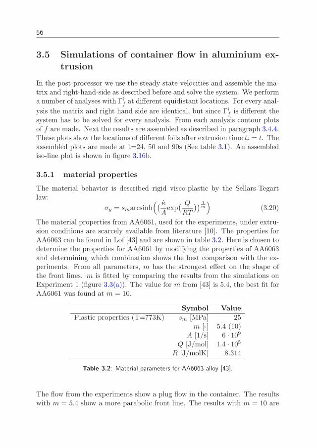
56
3.5 Simulations of container flow in aluminium ex-
trusion
In the post-processor we use the steady state velocities and assemble the ma-trix and right-hand-side as described before and solve the system. We performa number of analyses with Γi
f at different equidistant locations. For every anal-
ysis the matrix and right hand side are identical, but since Γif is different the
system has to be solved for every analysis. From each analysis contour plotsof f are made. Next the results are assembled as described in paragraph 3.4.4.These plots show the locations of different foils after extrusion time ti = t. Theassembled plots are made at t=24, 50 and 90s (See table 3.1). An assemblediso-line plot is shown in figure 3.16b.
3.5.1 material properties
The material behavior is described rigid visco-plastic by the Sellars-Tegartlaw:
σy = smarcsinh(
( κ
Aexp( Q
RT
))1
m
)
(3.20)
The material properties from AA6061, used for the experiments, under extru-sion conditions are scarcely available from literature [10]. The properties forAA6063 can be found in Lof [43] and are shown in table 3.2. Here is chosen todetermine the properties for AA6061 by modifying the properties of AA6063and determining which combination shows the best comparison with the ex-periments. From all parameters, m has the strongest effect on the shape ofthe front lines. m is fitted by comparing the results from the simulations onExperiment 1 (figure 3.3(a)). The value for m from [43] is 5.4, the best fit forAA6061 was found at m = 10.
Symbol Value
Plastic properties (T=773K) sm [MPa] 25m [-] 5.4 (10)
A [1/s] 6 · 109
Q [J/mol] 1.4 · 105
R [J/molK] 8.314
Table 3.2: Material parameters for AA6063 alloy [43].
The flow from the experiments show a plug flow in the container. The resultswith m = 5.4 show a more parabolic front line. The results with m = 10 are
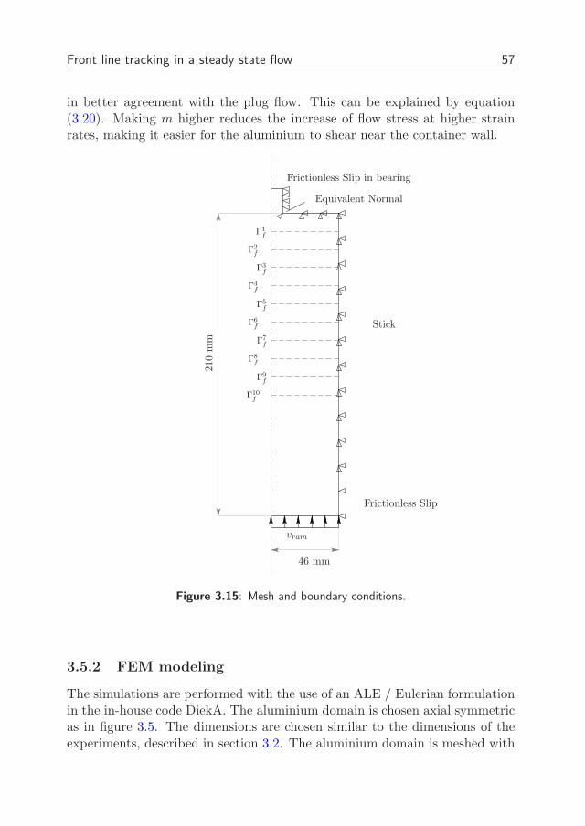
Front line tracking in a steady state flow 57
in better agreement with the plug flow. This can be explained by equation(3.20). Making m higher reduces the increase of flow stress at higher strainrates, making it easier for the aluminium to shear near the container wall.
Γ1f
Γ2f
Γ3f
Γ4f
Γ5f
Γ6f
Γ7f
Γ8f
Γ9f
Γ10f
Stick
Frictionless Slip
Equivalent Normal
Frictionless Slip in bearing
210
mm
46 mm
vram
Figure 3.15: Mesh and boundary conditions.
3.5.2 FEM modeling
The simulations are performed with the use of an ALE / Eulerian formulationin the in-house code DiekA. The aluminium domain is chosen axial symmetricas in figure 3.5. The dimensions are chosen similar to the dimensions of theexperiments, described in section 3.2. The aluminium domain is meshed with
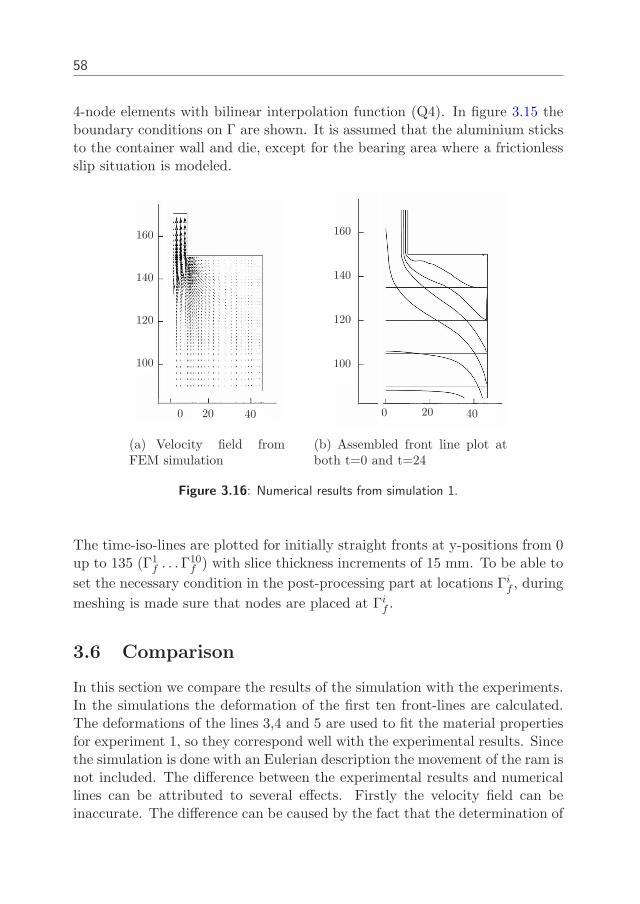
58
4-node elements with bilinear interpolation function (Q4). In figure 3.15 theboundary conditions on Γ are shown. It is assumed that the aluminium sticksto the container wall and die, except for the bearing area where a frictionlessslip situation is modeled.
0 20 40
100
120
140
160
(a) Velocity field fromFEM simulation
0 20 40
100
120
140
160
(b) Assembled front line plot atboth t=0 and t=24
Figure 3.16: Numerical results from simulation 1.
The time-iso-lines are plotted for initially straight fronts at y-positions from 0up to 135 (Γ1
f . . .Γ10f ) with slice thickness increments of 15 mm. To be able to
set the necessary condition in the post-processing part at locations Γif , during
meshing is made sure that nodes are placed at Γif .
3.6 Comparison
In this section we compare the results of the simulation with the experiments.In the simulations the deformation of the first ten front-lines are calculated.The deformations of the lines 3,4 and 5 are used to fit the material propertiesfor experiment 1, so they correspond well with the experimental results. Sincethe simulation is done with an Eulerian description the movement of the ram isnot included. The difference between the experimental results and numericallines can be attributed to several effects. Firstly the velocity field can beinaccurate. The difference can be caused by the fact that the determination of
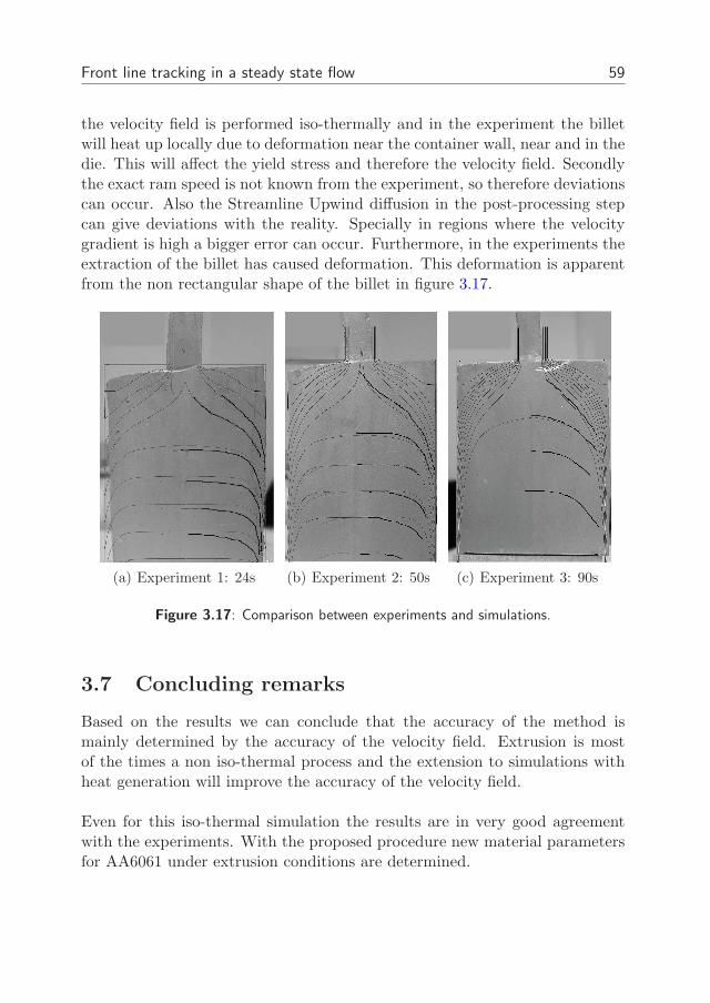
Front line tracking in a steady state flow 59
the velocity field is performed iso-thermally and in the experiment the billetwill heat up locally due to deformation near the container wall, near and in thedie. This will affect the yield stress and therefore the velocity field. Secondlythe exact ram speed is not known from the experiment, so therefore deviationscan occur. Also the Streamline Upwind diffusion in the post-processing stepcan give deviations with the reality. Specially in regions where the velocitygradient is high a bigger error can occur. Furthermore, in the experiments theextraction of the billet has caused deformation. This deformation is apparentfrom the non rectangular shape of the billet in figure 3.17.
(a) Experiment 1: 24s (b) Experiment 2: 50s (c) Experiment 3: 90s
Figure 3.17: Comparison between experiments and simulations.
3.7 Concluding remarks
Based on the results we can conclude that the accuracy of the method ismainly determined by the accuracy of the velocity field. Extrusion is mostof the times a non iso-thermal process and the extension to simulations withheat generation will improve the accuracy of the velocity field.
Even for this iso-thermal simulation the results are in very good agreementwith the experiments. With the proposed procedure new material parametersfor AA6061 under extrusion conditions are determined.

60
Chapter 4
Flow front tracking
During filling of the die at the startup of the extrusion process, the locationand velocity of the flow front will have a great influence on the deformationof the die. This especially applies to porthole dies. This deformation duringinitial filling will affect the performance of the die in the rest of the process.
When die correctors work on the die after trial pressings, their main informa-tion where to improve the die comes from the shape of the nose piece. Whenassessing a die numerically by FEM analysis the prediction of the shape of thenose piece can provide the same information. The prediction of the nose pieceshape requires the simulation of the full transient start-up of the process. Thisincludes the filling of the die.
In general an analysis of the filling stage requires the solution of the flow equa-tions and tracking the free surface or interface. The many interface trackingmethods can be categorized in two groups. Lagrangian methods are based ona moving mesh and Eulerian strategies are based on a fixed mesh. In Floryan& Rasmussen [20] an overview of various existing methods and their limita-tions is given.
In moving mesh strategies the material domain is meshed and the mesh de-forms according to the material. The free surface is represented by the freeboundary of the mesh. In processes with high deformations, like e.g. extru-sion, this strategy is limited by mesh distortion and contact problems. Theunavoidable remeshing and searching for contact areas makes this strategyinflexible and time consuming.
62
In fixed mesh strategies the complete domain is meshed and material withthe interface flows through the mesh. In extrusion the domain exists of a partof the billet, the die cavity and a part of the profile. In regions where highgradients are expected the mesh can be refined. The difficulty of fixed meshmethods is the tracking of the interface. In the next section interface trackingmethods are described.
A fixed mesh method is preferred because time consuming remeshing can beavoided. Besides that, when during the simulation the die is filled a fixed meshstrategy will converge to the steady state.
4.1 Flow front tracking algorithms
The three most popular strategies for tracking are the volume of fluid method(VOF) [27], the level set method [51,59] and the pseudo-concentration method[63, 64]. In all approaches the function φ is transported using the convectionequation
∂φ
∂t+ u∇φ = 0 (4.1)
With u the velocity field. It is well known in literature that the Galerkin for-mulation of equation (4.1) gives non-physical oscillations. Adding numericalstabilization can prevent this effect.
In VOF the function φ(x, y, z) indicates the fraction of a fluid in a cell. Ifφ = 1 the cell is filled with fluid A, if φ = 0 the cell is filled with fluid B. Theinterface is at 0 < φ < 1. There are several ways to transport this function.The main advantage in the VOF method is that the volume conservation isensured, however reconstruction of the interface is time consuming and com-plex for 3D cases [12].
In 1986 Thompson introduced the pseudo-concentration method [63], [64] totrack interfaces in two phase flows. The pseudo concentration method uses afunction φ that is 1 for fluid A and 0 for fluid B. At φ = 0.5 the interface canbe found. The material properties are calculated as:
µ = φµA + (1 − φ)µB (4.2)
The main disadvantage of both pseudo-concentration function and VOF meth-ods is the steep gradient in the φ-field that will be diffused in the numericalprocedures. To minimize these effect mesh refinements have been proposed in
Flow front tracking 63
the proximity of the interface [24,62,73].
The discontinuity of the pseudo-concentration function around the flow frontintroduces inaccuracies or oscillations during the convection through the FEMmesh. Dvorkin [18] already notices that if the initial distribution of the con-centration function is smooth enough, no smoothing algorithm is necessarylater in the simulation.
In the level set method the function φ is an initial smooth function. In [48]the best initial function for φ was found to be a signed distance from the front.The zero level set of the function φ = 0 defines the interface. The drawback ofthe level set method is, as in the pseudo- concentration function, that it doesnot ensured volume conservation rigorously. Besides that describing complexinitial interfaces with one distance function is difficult. In level set methodsseveral regularization algorithms of the distance function φ have been pro-posed [59,60].
In the next section a method is described that resembles the level set method.However the distance function φ is build from two or three (2D or 3D) initiallinear functions: The original coordinates.
4.2 Original coordinate tracking
In this section a new way to describe an interface is defined. The interface isno longer described by one field, but can be described by several fields. Thechosen initial fields should be smooth and easy to convect. As concentrationfunctions we chose the initially linear functions of the original coordinates.The original coordinate X0 in node n is calculated by subtracting the materialdisplacement un
m from the current coordinate Xn.
Xn0 = Xn − un
m (4.3)
This can be done in two or three directions, according to the dimension of thesimulation. For example the location of an initial circular interface in a 2Dsimulation with center (0,0) and radius R can be described as the zero levelof φ in equation (4.4).
φ = R2 −[
(X0 − Xcent)2 + (Y0 − Ycent)
2]
(4.4)
[Xcent, Ycent] is the location of the initial centre of the circular interface. Inthis scheme not the function φ is convected but the separate total displace-
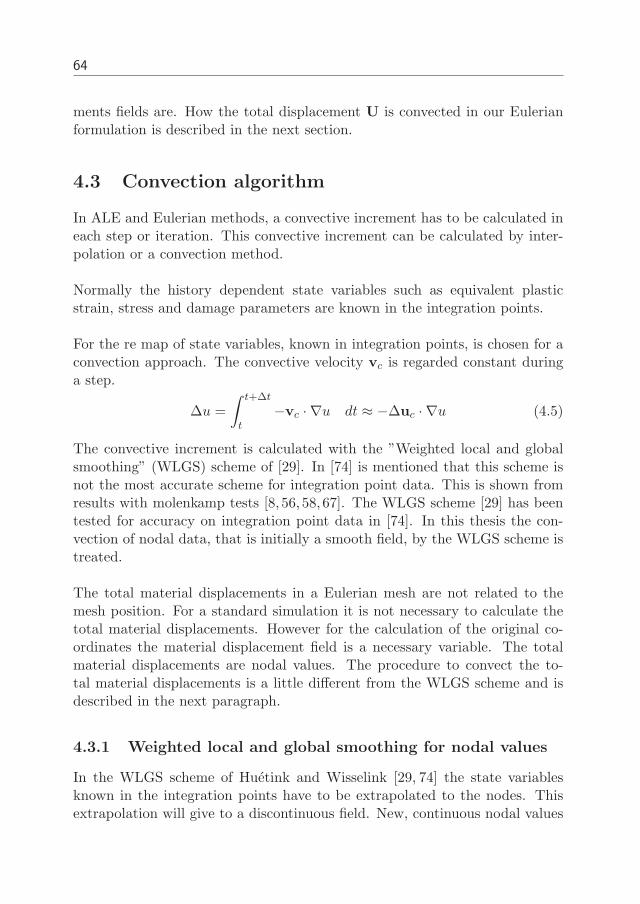
64
ments fields are. How the total displacement U is convected in our Eulerianformulation is described in the next section.
4.3 Convection algorithm
In ALE and Eulerian methods, a convective increment has to be calculated ineach step or iteration. This convective increment can be calculated by inter-polation or a convection method.
Normally the history dependent state variables such as equivalent plasticstrain, stress and damage parameters are known in the integration points.
For the re map of state variables, known in integration points, is chosen for aconvection approach. The convective velocity vc is regarded constant duringa step.
∆u =
∫ t+∆t
t
−vc · ∇u dt ≈ −∆uc · ∇u (4.5)
The convective increment is calculated with the ”Weighted local and globalsmoothing” (WLGS) scheme of [29]. In [74] is mentioned that this scheme isnot the most accurate scheme for integration point data. This is shown fromresults with molenkamp tests [8, 56, 58, 67]. The WLGS scheme [29] has beentested for accuracy on integration point data in [74]. In this thesis the con-vection of nodal data, that is initially a smooth field, by the WLGS scheme istreated.
The total material displacements in a Eulerian mesh are not related to themesh position. For a standard simulation it is not necessary to calculate thetotal material displacements. However for the calculation of the original co-ordinates the material displacement field is a necessary variable. The totalmaterial displacements are nodal values. The procedure to convect the to-tal material displacements is a little different from the WLGS scheme and isdescribed in the next paragraph.
4.3.1 Weighted local and global smoothing for nodal values
In the WLGS scheme of Huetink and Wisselink [29, 74] the state variablesknown in the integration points have to be extrapolated to the nodes. Thisextrapolation will give to a discontinuous field. New, continuous nodal values
Flow front tracking 65
are calculated by nodal averaging. Using this continuous field the new integra-tion point values are subsequently calculated based on a convection scheme.This scheme will add the global smoothing. This scheme has been treated inchapter 2.
For the total material displacements another scheme is used. In figure 4.1the WLGS for nodal values is shown. First the nodal values are ”extrap-olated” to the nodes. After this extrapolation the nodal value are averagedto create a new continuous field. These two steps are the equivalent of thelocal smoothing step for integration point data. Both steps are shown in figure4.1(a).
n1 n2 n3 n4
Before local smoothing:dknode
After local smoothing:denode
r
βrr
(a) Local smoothing and nodal averaging
n1 n2 n3 n4
After local smoothing:denode
nnew1 nnew
2 nnew3 nnew
4
After remap:dnewnode
(b) Remap of nodal values
Figure 4.1: Weighted Local and Global smoothing for nodal values.
Next the values in the new nodal locations are calculated by interpolation.This is shown in figure 4.1(b). Finally the new nodal values are avergaredto get the new smooth nodal field. These four steps are written in equations
66
(4.6) and (4.8).
denode =
n∑
k=1
Nk(βrr, βzz, βhh)dknode; (4.6)
With r,z,h the location of the nodes in isoparametic (local) coordinates of anelement. To prevent cross- wind diffusion the parameters βr, βz, βh can bechosen as [74]
βr = (1 − Cr), . . . (4.7)
The new discontinuous field is then averaged.
d?node =
1
ne
ne∑
k=1
denode
k (4.8)
The smoothed nodal values are remapped to the new mesh location as in4.1(b). In (4.9) this interpolation scheme is used to calculate the new nodalvalues.
dnewnode =
n∑
k=1
Nk((r, z, h)old − (Cr, Cz, Ch))d?node
k (4.9)
In these equations n is the number of nodes to one element and ne is thenumber of elements attached to one node. After the convection step the nodalvalues are discontinuous. The final step is nodal averaging to create a contin-uous field.
When the incremental displacements are equal to zero (Cr=0,. . . ), then dnewnode =
denode.
Courant number
The courant number is defined as the difference in local coordinates betweenthe old and new integration points, divided by the elements size(2x2x2 inlocal coordinates). The three Courant numbers are calculated for the differentdirections at every integration point. The integration point values are thenaveraged to one value for the whole element.
Cr =1
nip
nip∑
i=1
|∆rip|l
(4.10)
and the total courant number
C =√
C2r + C2
z + C2h (4.11)
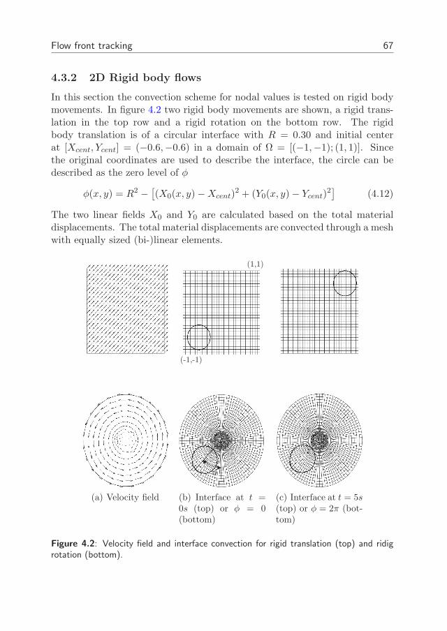
Flow front tracking 67
4.3.2 2D Rigid body flows
In this section the convection scheme for nodal values is tested on rigid bodymovements. In figure 4.2 two rigid body movements are shown, a rigid trans-lation in the top row and a rigid rotation on the bottom row. The rigidbody translation is of a circular interface with R = 0.30 and initial centerat [Xcent, Ycent] = (−0.6,−0.6) in a domain of Ω = [(−1,−1); (1, 1)]. Sincethe original coordinates are used to describe the interface, the circle can bedescribed as the zero level of φ
φ(x, y) = R2 −[
(X0(x, y) − Xcent)2 + (Y0(x, y) − Ycent)
2]
(4.12)
The two linear fields X0 and Y0 are calculated based on the total materialdisplacements. The total material displacements are convected through a meshwith equally sized (bi-)linear elements.
(a) Velocity field
(-1,-1)
(1,1)
φ
(b) Interface at t =0s (top) or φ = 0(bottom)
(c) Interface at t = 5s(top) or φ = 2π (bot-tom)
Figure 4.2: Velocity field and interface convection for rigid translation (top) and ridigrotation (bottom).
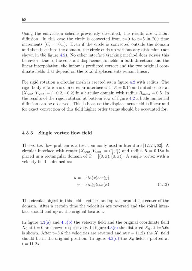
68
Using the convection scheme previously described, the results are withoutdiffusion. In this case the circle is convected from t=0 to t=5 in 200 timeincrements (Cr = 0.1). Even if the circle is convected outside the domainand then back into the domain, the circle ends up without any distortion (notshown in the figure 4.2). No other interface tracking method does posses thisbehavior. Due to the constant displacements fields in both directions and thelinear interpolation, the inflow is predicted correct and the two original coor-dinate fields that depend on the total displacements remain linear.
For rigid rotation a circular mesh is created as in figure 4.2 with radius. Therigid body rotation is of a circular interface with R = 0.15 and initial center at[Xcent, Ycent] = (−0.2,−0.2) in a circular domain with radius Rmesh = 0.5. Inthe results of the rigid rotation at bottom row of figure 4.2 a little numericaldiffusion can be observed. This is because the displacement field is linear andfor exact convection of this field higher order terms should be accounted for.
4.3.3 Single vortex flow field
The vortex flow problem is a test commonly used in literature [12, 24, 62]. Acircular interface with center [Xcent, Ycent] = (π
2 , π4 ) and radius R = 0.18π is
placed in a rectangular domain of Ω = [(0, π); (0, π)]. A single vortex with avelocity field is defined as:
u = −sin(x)cos(y)
v = sin(y)cos(x) (4.13)
The circular object in this field stretches and spirals around the center of thedomain. After a certain time the velocities are reversed and the spiral inter-face should end up at the original location.
In figure 4.3(a) and 4.3(b) the velocity field and the original coordinate fieldX0 at t = 0 are shown respectively. In figure 4.3(c) the distorted X0 at t=5.6sis shown. After t=5.6 the velocities are reversed and at t = 11.2s the X0 fieldshould be in the original position. In figure 4.3(d) the X0 field is plotted att = 11.2s.
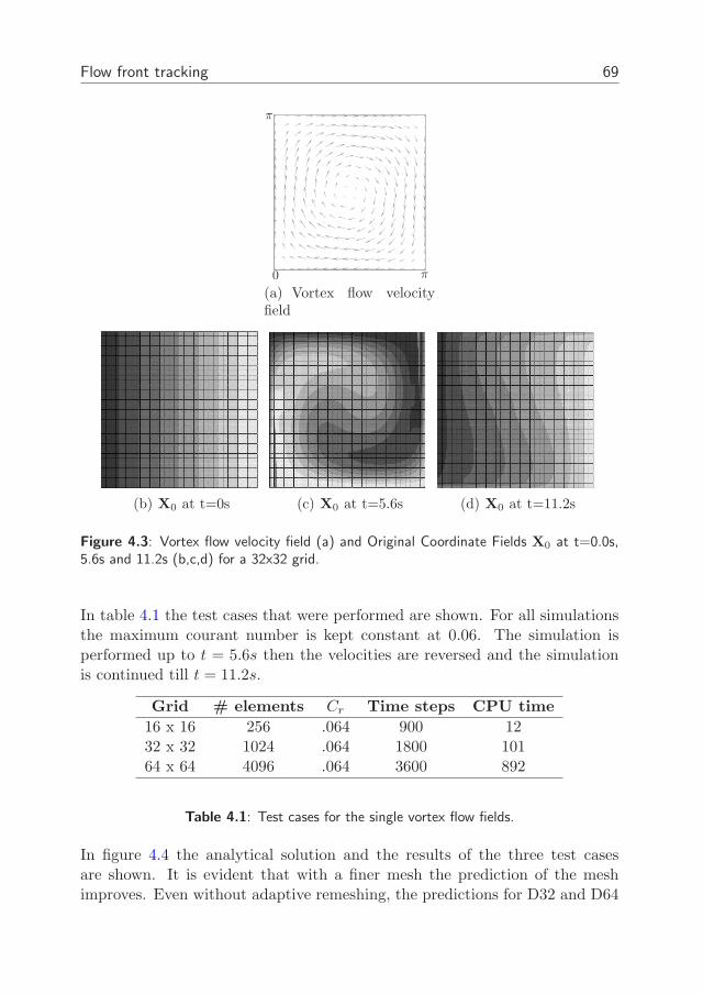
Flow front tracking 69
0
π
π
(a) Vortex flow velocityfield
(b) X0 at t=0s (c) X0 at t=5.6s (d) X0 at t=11.2s
Figure 4.3: Vortex flow velocity field (a) and Original Coordinate Fields X0 at t=0.0s,5.6s and 11.2s (b,c,d) for a 32x32 grid.
In table 4.1 the test cases that were performed are shown. For all simulationsthe maximum courant number is kept constant at 0.06. The simulation isperformed up to t = 5.6s then the velocities are reversed and the simulationis continued till t = 11.2s.
Grid # elements Cr Time steps CPU time
16 x 16 256 .064 900 1232 x 32 1024 .064 1800 10164 x 64 4096 .064 3600 892
Table 4.1: Test cases for the single vortex flow fields.
In figure 4.4 the analytical solution and the results of the three test casesare shown. It is evident that with a finer mesh the prediction of the meshimproves. Even without adaptive remeshing, the predictions for D32 and D64
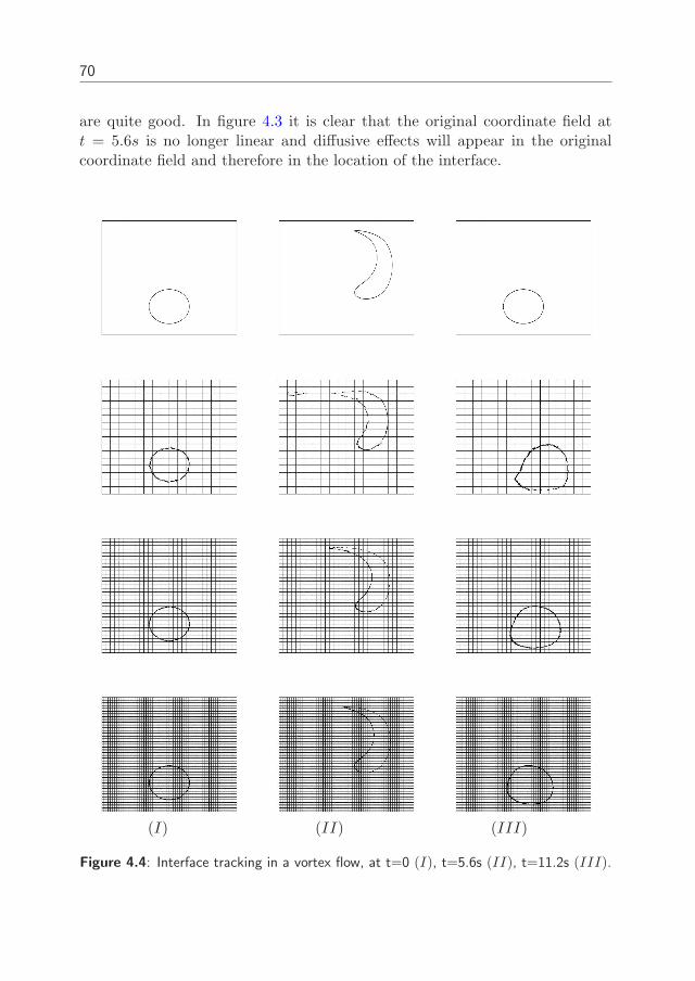
70
are quite good. In figure 4.3 it is clear that the original coordinate field att = 5.6s is no longer linear and diffusive effects will appear in the originalcoordinate field and therefore in the location of the interface.
(I) (II) (III)
Figure 4.4: Interface tracking in a vortex flow, at t=0 (I), t=5.6s (II), t=11.2s (III).
Flow front tracking 71
From these results can be concluded that the convection scheme in combi-nation with the original coordinate tracking shown good agreement with theanalytical location of the interface. The results in 16x16 grid are somewhatoscillatory, but taking the coarseness of the grid into account, the results arereasonable. Mesh refinement shows that the numerical results converge to theexact solution.
4.4 Numerical model
In the previous section the accuracy of the original coordinate interface track-ing scheme was demonstrated. In this section the numerical framework, spe-cific for interface tracking is shown. These specific features concern the updateof material properties during the simulation, boundary conditions and the de-scription of the interface during extrusion.
4.4.1 Interface description for extrusion
At the start of an extrusion process the die is still filled with air and the frontof a billet is straight and perpendicular to the extrusion direction. This makesthe definition of the interface in original coordinates very simple. A function,dependent on the original coordinate X0 in extrusion direction and a initiallocation of the front Xini is defined.
φ = Xini − X0 (4.14)
For this specific application the function itself could be seen as a typical levelset function. However not the function is convected but the total displace-ments are convected. The total displacements are initially constant equal tozero, whereas the initial level set function is linear. From the previous convec-tion tests can be concluded that the convection of a constant field shows lessdiffusion that the convection of a linear field.
Through convection high gradients can appear the function φ. These highgradients will deteriorate the accuracy of the convection of the function. Inmany level set approaches the function is regularized to stay a distance func-tion from the interface.
This is not the case for the original coordinate fuction. This function is regu-larized in such a manner that it will remain the original coordinate function. Inparagraph the regularization technique used for the original coordinate func-tion is treated.
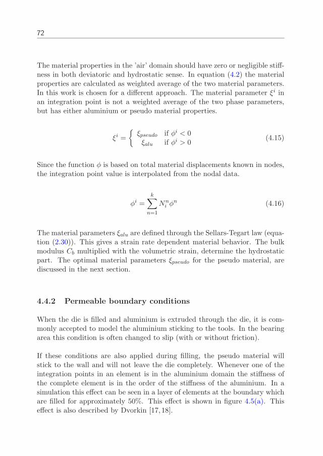
72
The material properties in the ’air’ domain should have zero or negligible stiff-ness in both deviatoric and hydrostatic sense. In equation (4.2) the materialproperties are calculated as weighted average of the two material parameters.In this work is chosen for a different approach. The material parameter ξi inan integration point is not a weighted average of the two phase parameters,but has either aluminium or pseudo material properties.
ξi =
ξpseudo if φi < 0ξalu if φi > 0
(4.15)
Since the function φ is based on total material displacements known in nodes,the integration point value is interpolated from the nodal data.
φi =k∑
n=1
Nni φn (4.16)
The material parameters ξalu are defined through the Sellars-Tegart law (equa-tion (2.30)). This gives a strain rate dependent material behavior. The bulkmodulus Cb multiplied with the volumetric strain, determine the hydrostaticpart. The optimal material parameters ξpseudo for the pseudo material, arediscussed in the next section.
4.4.2 Permeable boundary conditions
When the die is filled and aluminium is extruded through the die, it is com-monly accepted to model the aluminium sticking to the tools. In the bearingarea this condition is often changed to slip (with or without friction).
If these conditions are also applied during filling, the pseudo material willstick to the wall and will not leave the die completely. Whenever one of theintegration points in an element is in the aluminium domain the stiffness ofthe complete element is in the order of the stiffness of the aluminium. In asimulation this effect can be seen in a layer of elements at the boundary whichare filled for approximately 50%. This effect is shown in figure 4.5(a). Thiseffect is also described by Dvorkin [17,18].
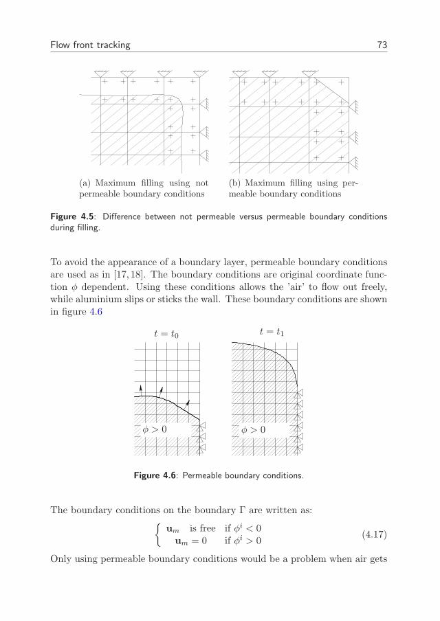
Flow front tracking 73
(a) Maximum filling using notpermeable boundary conditions
(b) Maximum filling using per-meable boundary conditions
Figure 4.5: Difference between not permeable versus permeable boundary conditionsduring filling.
To avoid the appearance of a boundary layer, permeable boundary conditionsare used as in [17,18]. The boundary conditions are original coordinate func-tion φ dependent. Using these conditions allows the ’air’ to flow out freely,while aluminium slips or sticks the wall. These boundary conditions are shownin figure 4.6
t = t0 t = t1
φ > 0φ > 0
Figure 4.6: Permeable boundary conditions.
The boundary conditions on the boundary Γ are written as:
um is free if φi < 0um = 0 if φi > 0
(4.17)
Only using permeable boundary conditions would be a problem when air gets
74
trapped inside the aluminium. This can happen if porthole dies are used andaluminium has to weld together after it has passed the portholes. This effectcan also appear during simulations. Therefore also the pseudo material shouldbe adjusted so that it is compressible.
Another advantage of the permeable boundary conditions is the ability touse bigger time increments during the first part of filling. The material veloc-ity is highest in the region upwind from the bearing area. Also the gradientsare high in that region. Therefore the mesh is refined in this region. It is clearthat the highest courant numbers are found there. The maximum step sizefor the model is determined by those elements. Using permeable boundaryconditions the high exit velocity at the bearing area vanishes. The pseudomaterial is then not forced to leave the domain through the bearing area, butcan flow out everywhere downstream from the front. This effect will lead tosmaller courant numbers and the ability to use bigger increments.
4.4.3 Modeling the pseudo material
The pseudo material can be modeled in many different ways. In literature onlythe viscosity is mentioned as specific pseudo parameter. Here we explored 26different models.
In simulation 0 (see table 4.2) the pseudo material is modeled as a viscousmaterial. The viscosity is chosen low with respect to the aluminium to ensurethat the pseudo material acts with low shearing forces on the aluminium. Tomake the pseudo material compressible the bulk modulus is also small com-pared to the aluminium bulk modulus.
In the other 25 simulations the material model for the pseudo material is an’adapted’ aluminium model (equation (2.30)) and bulk modulus. This adapt-ing of the parameters can be done on different levels in DiekA. In figure 4.7 asimplified scheme of the implementation of a FEM program is given. It is anincremental, iterative procedure as in figure 2.4(b). Within a time incrementDiekA iterates toward a solution of the non-linear equilibrium equations.
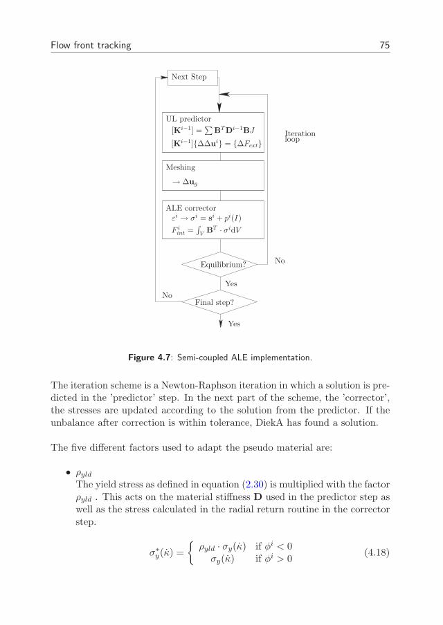
Flow front tracking 75
ALE corrector
Next Step
Equilibrium? No
No
Yes
Yes
Final step?
UL predictor
Meshing
→ ∆ug
Iterationloop
εi → σi = si + pi(I)
F iint =
∫
VBT · σidV
[Ki−1] =∑
BTDi−1BJ
[Ki−1]∆∆ui = ∆Fext
Figure 4.7: Semi-coupled ALE implementation.
The iteration scheme is a Newton-Raphson iteration in which a solution is pre-dicted in the ’predictor’ step. In the next part of the scheme, the ’corrector’,the stresses are updated according to the solution from the predictor. If theunbalance after correction is within tolerance, DiekA has found a solution.
The five different factors used to adapt the pseudo material are:
• ρyld
The yield stress as defined in equation (2.30) is multiplied with the factorρyld . This acts on the material stiffness D used in the predictor step aswell as the stress calculated in the radial return routine in the correctorstep.
σ∗y(κ) =
ρyld · σy(κ) if φi < 0σy(κ) if φi > 0
(4.18)
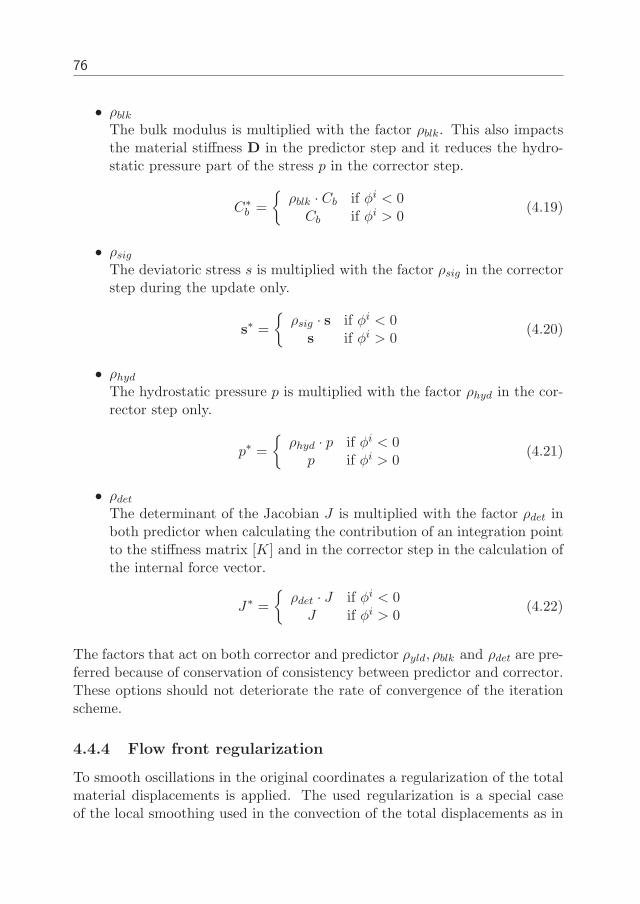
76
• ρblk
The bulk modulus is multiplied with the factor ρblk. This also impactsthe material stiffness D in the predictor step and it reduces the hydro-static pressure part of the stress p in the corrector step.
C∗b =
ρblk · Cb if φi < 0Cb if φi > 0
(4.19)
• ρsig
The deviatoric stress s is multiplied with the factor ρsig in the correctorstep during the update only.
s∗ =
ρsig · s if φi < 0s if φi > 0
(4.20)
• ρhyd
The hydrostatic pressure p is multiplied with the factor ρhyd in the cor-rector step only.
p∗ =
ρhyd · p if φi < 0p if φi > 0
(4.21)
• ρdet
The determinant of the Jacobian J is multiplied with the factor ρdet inboth predictor when calculating the contribution of an integration pointto the stiffness matrix [K] and in the corrector step in the calculation ofthe internal force vector.
J∗ =
ρdet · J if φi < 0J if φi > 0
(4.22)
The factors that act on both corrector and predictor ρyld, ρblk and ρdet are pre-ferred because of conservation of consistency between predictor and corrector.These options should not deteriorate the rate of convergence of the iterationscheme.
4.4.4 Flow front regularization
To smooth oscillations in the original coordinates a regularization of the totalmaterial displacements is applied. The used regularization is a special caseof the local smoothing used in the convection of the total displacements as in
Flow front tracking 77
equation (4.6). The regularization is performed when convergence rate of theglobal iteration slows down.
v
(a) Oscillations in theoriginal coordinates
v
(b) Element averagedvalues
v
(c) regulated original co-ordinates after nodal aver-aging
Figure 4.8: Regularization of the flow front.
For all elements the element average value for original coordinates is calcu-lated and written to the nodes as in figure 4.8(b). The created discontinuousfield is made continuous by nodal averaging. This creates the field as in figure4.8(c). Note that extra boundary conditions appear by this regularization step.
With the factor β from equation (4.7) the smoothing can be less radical asusing the element average as nodal values. In our implementation, when asmoothing step is applied the element average is put in the nodes. (β = 0).In the next section in figure 4.20 is shown that this improves the volume con-servation behavior drastically. Also an improvement in convergence speed isobserved.
4.5 2D filling of Die cavity
In this section a comparison is made of different option to model the pseudomaterial. Different values and combinations of the factors from paragraph4.4.3 are used.
The geometry for the test is a 2D plane strain model and is shown in figure
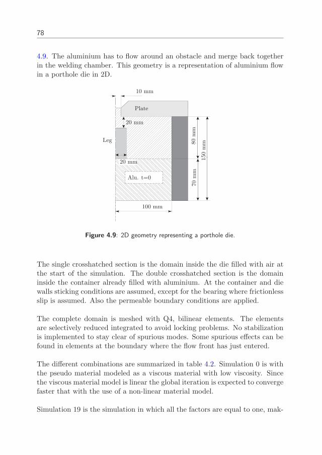
78
4.9. The aluminium has to flow around an obstacle and merge back togetherin the welding chamber. This geometry is a representation of aluminium flowin a porthole die in 2D.
10 mm
150
mm
100 mm
80m
m70
mm
20 mm
20 mm
Alu. t=0
Leg
Plate
Figure 4.9: 2D geometry representing a porthole die.
The single crosshatched section is the domain inside the die filled with air atthe start of the simulation. The double crosshatched section is the domaininside the container already filled with aluminium. At the container and diewalls sticking conditions are assumed, except for the bearing where frictionlessslip is assumed. Also the permeable boundary conditions are applied.
The complete domain is meshed with Q4, bilinear elements. The elementsare selectively reduced integrated to avoid locking problems. No stabilizationis implemented to stay clear of spurious modes. Some spurious effects can befound in elements at the boundary where the flow front has just entered.
The different combinations are summarized in table 4.2. Simulation 0 is withthe pseudo material modeled as a viscous material with low viscosity. Sincethe viscous material model is linear the global iteration is expected to convergefaster that with the use of a non-linear material model.
Simulation 19 is the simulation in which all the factors are equal to one, mak-
Flow front tracking 79
ing the pseudo material properties equal to the aluminium properties. This isfor simulation times the reference simulation. Without the permeable bound-ary conditions this would be a regular extrusion simulation.
Two different mechanisms occur. The first mechanism shows the oscillationsof figure 4.8(a). The other effect is also observed at the edge of the domain.When in an element at the edge of the domain both the interface has enteredand one node stays permeable while the other is changed to fixed, the per-meable node can have a (large) spurious displacement. When this happens insome subsequent increments the element fills up too fast.
4.5.1 Results of 2D die filling
The best option will be chosen based on the results of volume conservation,flow front shape, ability to fill corners and the simulation times.
Table 4.2: Simulations.Simulation ρyld ρblk ρsig ρhyd ρdet run
0 Viscous, µ = 10−6m2s−1 , Cb = 1MPa OK1 0.1 1.0 1.0 1.0 1.0 Incomplete2 0.01 1.0 1.0 1.0 1.0 Fails3 0.001 1.0 1.0 1.0 1.0 Fails4 1.0 0.1 1.0 1.0 1.0 OK5 1.0 0.01 1.0 1.0 1.0 OK6 1.0 0.001 1.0 1.0 1.0 OK7 0.01 0.01 1.0 1.0 1.0 Incomplete8 0.01 0.001 1.0 1.0 1.0 OK9 0.01 0.00001 1.0 1.0 1.0 Fails10 1.0 1.0 1.0 1.0 0.1 OK11 1.0 1.0 1.0 1.0 0.01 Incomplete12 1.0 1.0 1.0 1.0 0.001 Incomplete13 1.0 1.0 0.667 1.0 1.0 OK14 1.0 1.0 0.333 1.0 1.0 OK15 1.0 1.0 0.000 1.0 1.0 Fails16 1.0 1.0 -0.333 1.0 1.0 Fails17 1.0 1.0 -0.667 1.0 1.0 Fails18 1.0 1.0 -1.000 1.0 1.0 Fails19 1.0 1.0 1.0 1.0 1.0 OK20 1.0 1.0 1.0 0.667 1.0 OK21 1.0 1.0 1.0 0.333 1.0 OK22 1.0 1.0 1.0 0.000 1.0 Fails23 1.0 1.0 1.0 -0.333 1.0 Fails24 1.0 1.0 1.0 -0.667 1.0 Fails25 1.0 1.0 1.0 -1.000 1.0 Fails
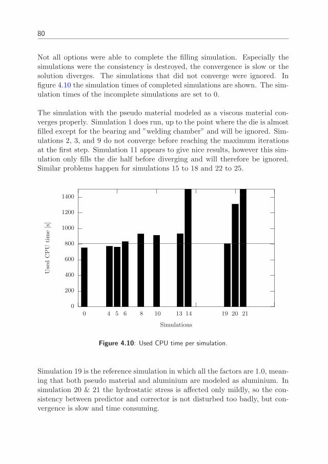
80
Not all options were able to complete the filling simulation. Especially thesimulations were the consistency is destroyed, the convergence is slow or thesolution diverges. The simulations that did not converge were ignored. Infigure 4.10 the simulation times of completed simulations are shown. The sim-ulation times of the incomplete simulations are set to 0.
The simulation with the pseudo material modeled as a viscous material con-verges properly. Simulation 1 does run, up to the point where the die is almostfilled except for the bearing and ”welding chamber” and will be ignored. Sim-ulations 2, 3, and 9 do not converge before reaching the maximum iterationsat the first step. Simulation 11 appears to give nice results, however this sim-ulation only fills the die half before diverging and will therefore be ignored.Similar problems happen for simulations 15 to 18 and 22 to 25.
0
200
400
600
800
1000
1200
1400
0 4 5 6 8 10 13 14 19 20 21
Use
dC
PU
tim
e[s
]
Simulations
”
Figure 4.10: Used CPU time per simulation.
Simulation 19 is the reference simulation in which all the factors are 1.0, mean-ing that both pseudo material and aluminium are modeled as aluminium. Insimulation 20 & 21 the hydrostatic stress is affected only mildly, so the con-sistency between predictor and corrector is not disturbed too badly, but con-vergence is slow and time consuming.
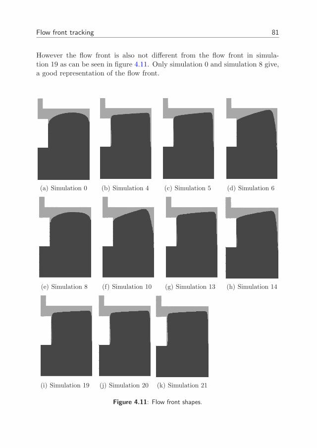
Flow front tracking 81
However the flow front is also not different from the flow front in simula-tion 19 as can be seen in figure 4.11. Only simulation 0 and simulation 8 give,a good representation of the flow front.
(a) Simulation 0 (b) Simulation 4 (c) Simulation 5 (d) Simulation 6
(e) Simulation 8 (f) Simulation 10 (g) Simulation 13 (h) Simulation 14
(i) Simulation 19 (j) Simulation 20 (k) Simulation 21
Figure 4.11: Flow front shapes.
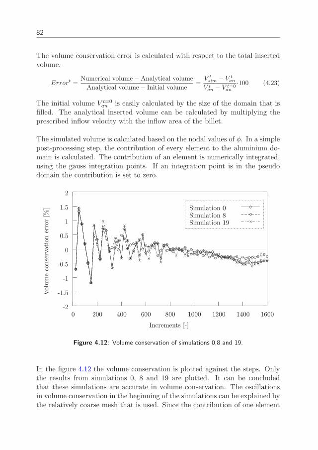
82
The volume conservation error is calculated with respect to the total insertedvolume.
Errort =Numerical volume − Analytical volume
Analytical volume − Initial volume=
V t
sim− V t
an
V tan
− V t=0an
·100 (4.23)
The initial volume V t=0an is easily calculated by the size of the domain that is
filled. The analytical inserted volume can be calculated by multiplying theprescribed inflow velocity with the inflow area of the billet.
The simulated volume is calculated based on the nodal values of φ. In a simplepost-processing step, the contribution of every element to the aluminium do-main is calculated. The contribution of an element is numerically integrated,using the gauss integration points. If an integration point is in the pseudodomain the contribution is set to zero.
-2
-1.5
-1
-0.5
0
0.5
1
1.5
2
0 200 400 600 800 1000 1200 1400 1600
Vol
um
eco
nse
rvat
ion
erro
r[%
]
Increments [-]
Simulation 0Simulation 8Simulation 19
Figure 4.12: Volume conservation of simulations 0,8 and 19.
In the figure 4.12 the volume conservation is plotted against the steps. Onlythe results from simulations 0, 8 and 19 are plotted. It can be concludedthat these simulations are accurate in volume conservation. The oscillationsin volume conservation in the beginning of the simulations can be explained bythe relatively coarse mesh that is used. Since the contribution of one element
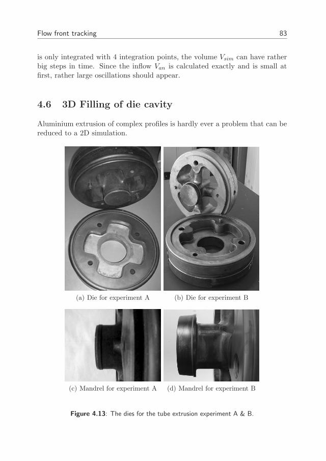
Flow front tracking 83
is only integrated with 4 integration points, the volume Vsim can have ratherbig steps in time. Since the inflow Van is calculated exactly and is small atfirst, rather large oscillations should appear.
4.6 3D Filling of die cavity
Aluminium extrusion of complex profiles is hardly ever a problem that can bereduced to a 2D simulation.
(a) Die for experiment A (b) Die for experiment B
(c) Mandrel for experiment A (d) Mandrel for experiment B
Figure 4.13: The dies for the tube extrusion experiment A & B.
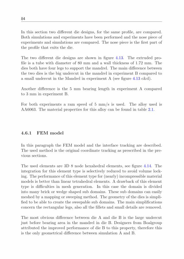
84
In this section two different die designs, for the same profile, are compared.Both simulations and experiments have been performed and the nose piece ofexperiments and simulations are compared. The nose piece is the first part ofthe profile that exits the die.
The two different die designs are shown in figure 4.13. The extruded pro-file is a tube with diameter of 80 mm and a wall thickness of 1.72 mm. Thedies both have four legs to support the mandrel. The main difference betweenthe two dies is the big undercut in the mandrel in experiment B compared toa small undercut in the Mandrel in experiment A (see figure 4.13 c&d).
Another difference is the 5 mm bearing length in experiment A comparedto 3 mm in experiment B.
For both experiments a ram speed of 5 mm/s is used. The alloy used isAA6063. The material properties for this alloy can be found in table 2.1.
4.6.1 FEM model
In this paragraph the FEM model and the interface tracking are described.The used method is the original coordinate tracking as prescribed in the pre-vious sections.
The used elements are 3D 8 node hexahedral elements, see figure 4.14. Theintegration for this element type is selectively reduced to avoid volume lock-ing. The performance of this element type for (nearly) incompressible materialmodels is better than linear tetrahedral elements. A drawback of this elementtype is difficulties in mesh generation. In this case the domain is dividedinto many brick or wedge shaped sub domains. These sub domains can easilymeshed by a mapping or sweeping method. The geometry of the dies is simpli-fied to be able to create the sweepable sub domains. The main simplificationsconcern the rectangular legs, also all the fillets and small details are removed.
The most obvious difference between die A and die B is the large undercutjust before bearing area in the mandrel in die B. Designers from Boalgroupattributed the improved performance of die B to this property, therefore thisis the only geometrical difference between simulation A and B.
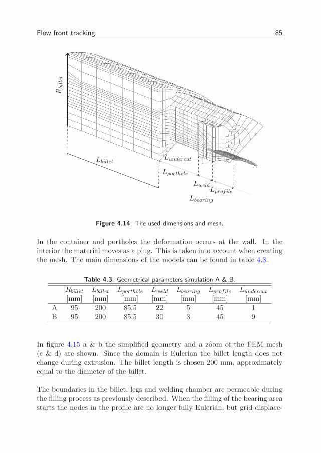
Flow front tracking 85
Rbi
llet
Lbillet
Lporthole
Lweld
Lbearing
Lprofile
Lundercut
Figure 4.14: The used dimensions and mesh.
In the container and portholes the deformation occurs at the wall. In theinterior the material moves as a plug. This is taken into account when creatingthe mesh. The main dimensions of the models can be found in table 4.3.
Table 4.3: Geometrical parameters simulation A & B.
Rbillet Lbillet Lporthole Lweld Lbearing Lprofile Lundercut
[mm] [mm] [mm] [mm] [mm] [mm] [mm]
A 95 200 85.5 22 5 45 1B 95 200 85.5 30 3 45 9
In figure 4.15 a & b the simplified geometry and a zoom of the FEM mesh(c & d) are shown. Since the domain is Eulerian the billet length does notchange during extrusion. The billet length is chosen 200 mm, approximatelyequal to the diameter of the billet.
The boundaries in the billet, legs and welding chamber are permeable duringthe filling process as previously described. When the filling of the bearing areastarts the nodes in the profile are no longer fully Eulerian, but grid displace-
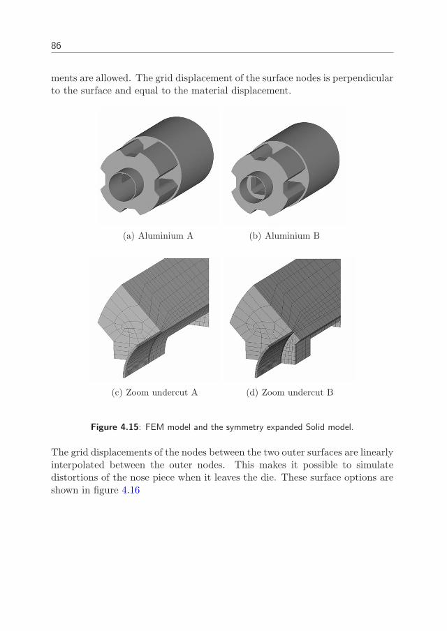
86
ments are allowed. The grid displacement of the surface nodes is perpendicularto the surface and equal to the material displacement.
(a) Aluminium A (b) Aluminium B
(c) Zoom undercut A (d) Zoom undercut B
Figure 4.15: FEM model and the symmetry expanded Solid model.
The grid displacements of the nodes between the two outer surfaces are linearlyinterpolated between the outer nodes. This makes it possible to simulatedistortions of the nose piece when it leaves the die. These surface options areshown in figure 4.16
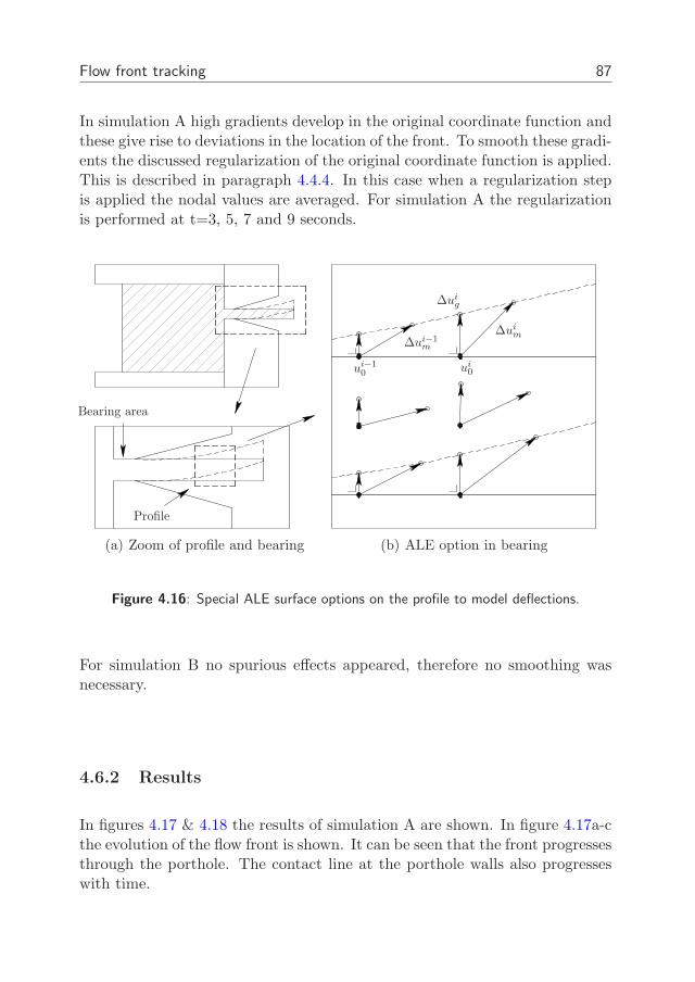
Flow front tracking 87
In simulation A high gradients develop in the original coordinate function andthese give rise to deviations in the location of the front. To smooth these gradi-ents the discussed regularization of the original coordinate function is applied.This is described in paragraph 4.4.4. In this case when a regularization stepis applied the nodal values are averaged. For simulation A the regularizationis performed at t=3, 5, 7 and 9 seconds.
Bearing area
Profile
(a) Zoom of profile and bearing
∆ui−1m
∆uim
∆uig
ui−10 ui
0
(b) ALE option in bearing
Figure 4.16: Special ALE surface options on the profile to model deflections.
For simulation B no spurious effects appeared, therefore no smoothing wasnecessary.
4.6.2 Results
In figures 4.17 & 4.18 the results of simulation A are shown. In figure 4.17a-cthe evolution of the flow front is shown. It can be seen that the front progressesthrough the porthole. The contact line at the porthole walls also progresseswith time.
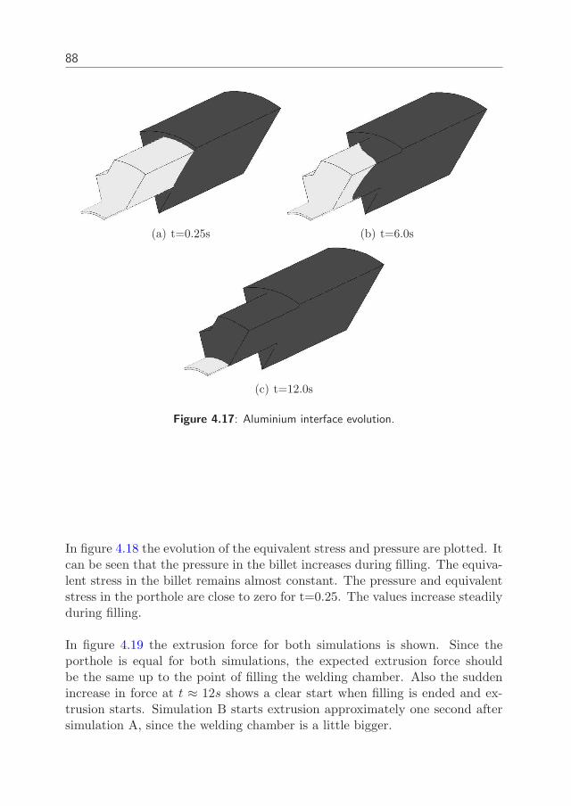
88
(a) t=0.25s (b) t=6.0s
(c) t=12.0s
Figure 4.17: Aluminium interface evolution.
In figure 4.18 the evolution of the equivalent stress and pressure are plotted. Itcan be seen that the pressure in the billet increases during filling. The equiva-lent stress in the billet remains almost constant. The pressure and equivalentstress in the porthole are close to zero for t=0.25. The values increase steadilyduring filling.
In figure 4.19 the extrusion force for both simulations is shown. Since theporthole is equal for both simulations, the expected extrusion force shouldbe the same up to the point of filling the welding chamber. Also the suddenincrease in force at t ≈ 12s shows a clear start when filling is ended and ex-trusion starts. Simulation B starts extrusion approximately one second aftersimulation A, since the welding chamber is a little bigger.
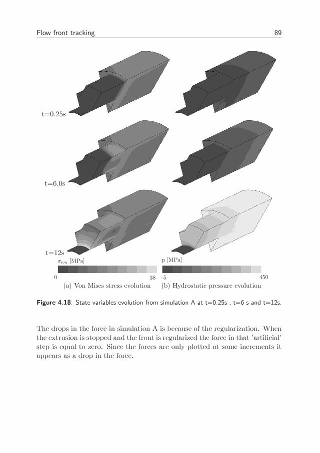
Flow front tracking 89
t=0.25s
t=6.0s
t=12s
380
σvm [MPa]
(a) Von Mises stress evolution
p [MPa]
450-5
(b) Hydrostatic pressure evolution
Figure 4.18: State variables evolution from simulation A at t=0.25s , t=6 s and t=12s.
The drops in the force in simulation A is because of the regularization. Whenthe extrusion is stopped and the front is regularized the force in that ’artificial’step is equal to zero. Since the forces are only plotted at some increments itappears as a drop in the force.
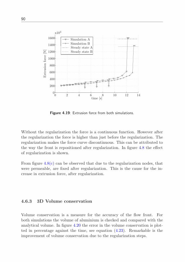
90
Extr
usi
onfo
rce
[N]
time [s]
Simulation ASimulation BSteady state ASteady state B
102 124 146 8
x103
00
1000
200
1200
400
1400
600
1600
800
Figure 4.19: Extrusion force from both simulations.
Without the regularization the force is a continuous function. However afterthe regularization the force is higher than just before the regularization. Theregularization makes the force curve discontinuous. This can be attributed tothe way the front is repositioned after regularization. In figure 4.8 the effectof regularization is shown.
From figure 4.8(c) can be observed that due to the regularization nodes, thatwere permeable, are fixed after regularization. This is the cause for the in-crease in extrusion force, after regularization.
4.6.3 3D Volume conservation
Volume conservation is a measure for the accuracy of the flow front. Forboth simulations the volume of aluminium is checked and compared with theanalytical volume. In figure 4.20 the error in the volume conservation is plot-ted in percentage against the time, see equation (4.23). Remarkable is theimprovement of volume conservation due to the regularization steps.
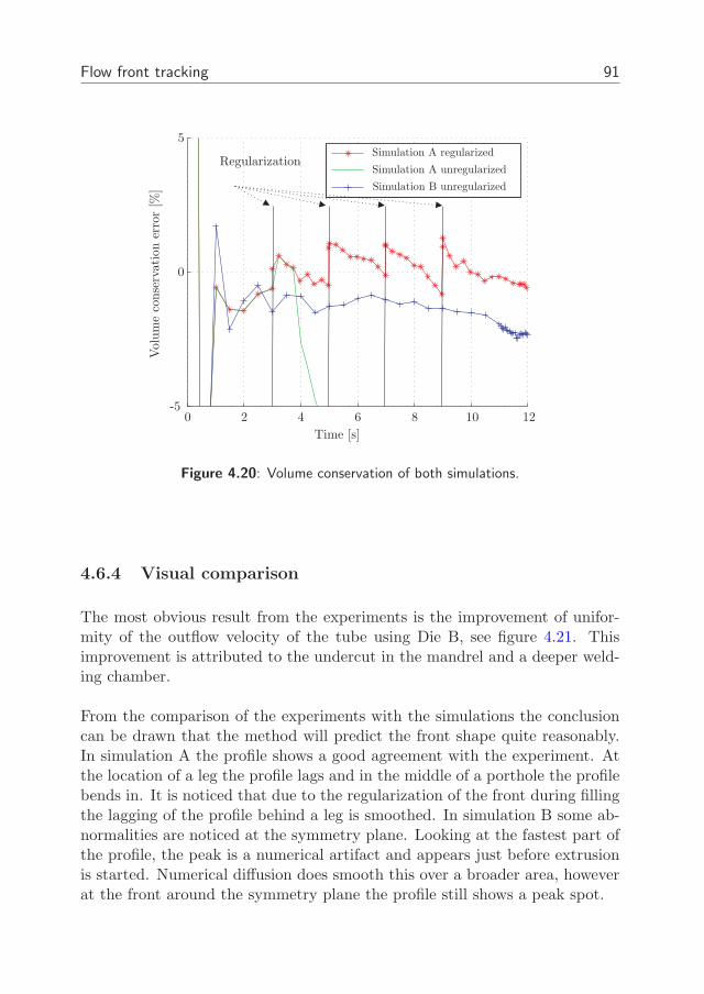
Flow front tracking 91
0
0 2 4
5
6 8 10 12
140
Simulation A regularized
Simulation A unregularized
Simulation B unregularized
Vol
um
eco
nse
rvat
ion
erro
r[%
]
Time [s]
-5
Regularization
Figure 4.20: Volume conservation of both simulations.
4.6.4 Visual comparison
The most obvious result from the experiments is the improvement of unifor-mity of the outflow velocity of the tube using Die B, see figure 4.21. Thisimprovement is attributed to the undercut in the mandrel and a deeper weld-ing chamber.
From the comparison of the experiments with the simulations the conclusioncan be drawn that the method will predict the front shape quite reasonably.In simulation A the profile shows a good agreement with the experiment. Atthe location of a leg the profile lags and in the middle of a porthole the profilebends in. It is noticed that due to the regularization of the front during fillingthe lagging of the profile behind a leg is smoothed. In simulation B some ab-normalities are noticed at the symmetry plane. Looking at the fastest part ofthe profile, the peak is a numerical artifact and appears just before extrusionis started. Numerical diffusion does smooth this over a broader area, howeverat the front around the symmetry plane the profile still shows a peak spot.
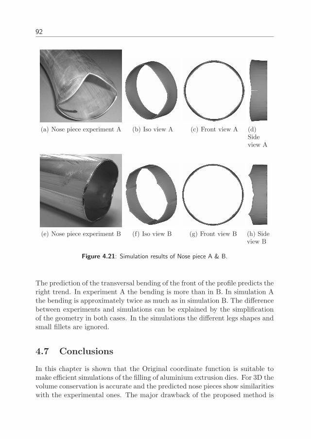
92
(a) Nose piece experiment A (b) Iso view A (c) Front view A (d)Sideview A
(e) Nose piece experiment B (f) Iso view B (g) Front view B (h) Sideview B
Figure 4.21: Simulation results of Nose piece A & B.
The prediction of the transversal bending of the front of the profile predicts theright trend. In experiment A the bending is more than in B. In simulation Athe bending is approximately twice as much as in simulation B. The differencebetween experiments and simulations can be explained by the simplificationof the geometry in both cases. In the simulations the different legs shapes andsmall fillets are ignored.
4.7 Conclusions
In this chapter is shown that the Original coordinate function is suitable tomake efficient simulations of the filling of aluminium extrusion dies. For 3D thevolume conservation is accurate and the predicted nose pieces show similaritieswith the experimental ones. The major drawback of the proposed method is

Flow front tracking 93
the use of the hexahedral elements. To be able to mesh the domain withtopological correct hexahedral elements, the geometry had to be simplified toan extend that no correct prediction of the nose piece could be expected. In thenext chapter the interface tracking algorithm is implemented in a tetrahedralelement. Meshing with tetrahedral elements allows the user to add much moredetail.

94
Chapter 5
A mixed finite element with
original coordinate tracking
Creating finite element meshes of complex geometries is often done by com-mercial software tools. Many of these packages prefer triangular or tetrahedralelements over quadrilateral or hexahedral elements. The automatic mesh gen-eration is easier for these elements. For computation time sake the elementsare to be of low order. This also makes contact issues less problematic.
Although low order elements have been available since decades, it is well knownthat they do not yield accurate results. Especially when an extra physicalconstraint of (nearly) incompressibility is added, volume locking occurs. Thisfailure may be assessed numerically by patch tests [32, 76] or mathematicallyverified by the Babuska-Brezzi condition [7].A possibility to improve standard linear elements is by adding extra degrees offreedom such as pressure or strains. The degrees of freedom consist of a mix ofdisplacement and other degrees of freedom: a mixed element. This techniquewas first introduced by Herrmann [26] and Chorin [11] to solve nearly in-compressible linear elastic problems and incompressible viscous flow problemsrespectively. Later Schneider [57] introduced equal order interpolations fordisplacement field and pressure field, regarding both fields as separate fields.When both pressure and displacement fields are chosen linear and continuous,it is well known that these elements fail the patch tests [75].
One way to stabilize the pressure field is to augment the linear displacementinterpolation functions by a bubble function. This was first introduced byArnold et. al. [4] to solve the stokes problem. This type of element is called
96
MINI element. In this thesis MINI elements are referred to as T3P1+P1 (tri-angular) and T4P1+P1 (tetrahedral). Coupez et. al. [22, 53] uses an elementfrom the MINI family to solve 3D mold filling problems for viscous incom-pressible fluids. The bubble displacements are four piecewise linear functionsto maintain exact integration property of the element. Coupez solves thetransport equation decoupled from the flow problem. Taylor [61] introducedthe use of bubbles in a mixed-enhanced tetrahedral element for small and fi-nite elastic strains.
Meshing and contact problems are easier with linear triangles or tetrahedralelements. From the literature in the above paragraphs the behavior of theMINI elements show good results. However not much literature about theuse of MINI elements in ALE formulations is available. In the next sections,our implementation of two MINI elements is described. In this chapter manydifferent Element types are mentioned by their abbreviation. In table 5.1 anoverview these elements and abbreviations is given.
Abbr. Elem. shape # nodes DOFS Interpolation
2D T3 Triangular 3 u,v linearQ4 Quadrilateral 4 u,v bi-linearT3P1+P1 Triangular 4 (3+1) u,v,p + u,v linear + bubble
3D TET4 Tetrahedral 4 u,v,w linearH8 Hexahedral 8 u,v,w, bi-linearT4P1+P1 Tetrahedral 5 (4+1) u,v,w,p + u,v,w linear + bubble
Table 5.1: Element types and abbreviations.
5.1 Theoretical outline
In chapter 2 the basic outline of a semi-coupled ALE simulation is shown.In the next sections the theoretical outline and implementation of a MINIelement in a semi-coupled ALE formulation are treated.
5.1.1 Strong formulation
The strong form of the equilibrium equations with the boundary conditions isgiven in equation (5.1).
σ · ∇ = 0 in Ωg
u = u0 on Γu
σ · n = t on Γt
(5.1)
A mixed finite element with original coordinate tracking 97
5.1.2 Weak formulation
Since a semi-coupled ALE description is used, the Updated Lagrangian for-mulation of the weak form is used in the predictor step. In Appendix A theweak form for an Updated Lagrangian formulation is derived. Here the resultis written as:
∫
Ωw
∇:(
− σ · LT + σ + σtrL)
dΩ =
∫
Γt
w · t dΓt +
∫
Γt
w · tJΓ dΓt (5.2)
5.2 FEM discretisation
The finite element method is applied to discretize the weak formulations. Thedomain is split into a finite number of sub domains. Integrals of the weakform are subdivided into a finite number of sub integrals. For each elementthe incremental displacement is described by the interpolation functions N
and the nodal incremental displacements ∆u. The pressure is interpolatedusing the interpolation functions M . Within one increment the velocity and(rate of the) pressure are assumed constant making v = ∆u
∆tand p =
∆p∆t
.
∆u =∑
∆uiNi ; x =∑
xiNi (5.3)
∆p =∑
∆piMi (5.4)
Ni are linear for the corner nodes and cubic or quartic for the bubble node.Since pi is chosen linear the shape functions Mi are linear shape functions andchosen identical to the linear part of Ni.
The derivation for the MINI element start with the same weak form as inparagraph 2.3.2. For the MINI elements the stresses are split into a deviatoricand a hydrostatic part. For the weighing functions the Galerkin method isapplied here, which means that the same interpolation functions used for thedisplacements are also used for the weighing functions.
w =∑
wiNi ; p∗ =∑
p∗i Mi (5.5)
L = v
∇=∑
viNi
∇ (5.6)
D =1
2
(
L + LT)
=∑ 1
2
(
viNi
∇ +
∇Nivi
)
=∑
Bivi (5.7)
98
And the same for the weighing functions:
L∗ = w
∇=∑
wiNi
∇ (5.8)
D∗ =1
2
(
L∗ + L∗T ) =∑ 1
2
(
wiNi
∇ +
∇Niwi
)
=∑
Biwi (5.9)
The Jaumann stress rate can be written as:
O
σ=O
s −p1 = Y : D − σ · W + W · σ − σtrD − p1 (5.10)
with Y = 2GI − 3Gss(1+h)σ2
y− 2
3G11. Equation (5.10) can be substituted into
equation (5.2):
∫
Ωw
∇:(
− σ · LT + Y : D − σ · W + W · σ)
dΩ −∫
Ωw
∇: p1dΩ = (5.11)
∫
Γt
w · t dΓt +
∫
Γt
w · tJΓ dΓt
This can be rewritten into:
∫
Ωw
∇:(
L · σ + (Y : D − σ · D − D · σ))
dΩ −∫
Ωw
∇: p1dΩ = (5.12)
∫
Γt
w · t dΓt +
∫
Γt
w · tJΓ dΓt
By using equations (5.3)-(5.9) and keeping the velocity and rate of pressureconstant during the increment we get:
∑
ij
wj
[
∫
ΩNj
∇: σ : Ni
∇ dΩ +
∫
ΩBT
j :(
Y − σ · I − I · σ)
: Bi dΩ
]
∆ui − wj
∫
ΩBT
j : 1Mi dΩ∆pi = (5.13)
∑
ij
wj
[
∫
Γt
Nj · ∆t dΓt +
∫
Γt
Nj · tJΓ dΓt
]
∀wj
A mixed finite element with original coordinate tracking 99
Which implies
∑
i
[
∫
ΩNj
∇: σ : Ni
∇ dΩ +
∫
ΩBT
j :(
Y − σ · I − I · σ)
: Bi dΩ
]
∆ui −∫
ΩBT
j : 1Mi dΩ∆pi = (5.14)
∑
i
[
∫
Γt
Nj · ∆t dΓt +
∫
Γt
Nj · tJΓ dΓt
]
The constraint for the constitutive equation of the pressure gives the secondequation:
∫
Ωp∗(
tr(D) +1
Cb
p
)
dΩ = 0 (5.15)
Using the interpolations functions gives and integration in time gives:
∑
ij
p∗j
[
∫
ΩMT
j 1 : Bi dΩui +1
Cb
∫
ΩMT
j Mi dΩpi
]
= 0 (5.16)
In this integration over time the volume strain is assumed to be elastic.
p = −Cb
∆v
v= −CbJ ≈
∑
i
1 : Biui (5.17)
With J = det(F) and F the deformation gradient tensor. The determinant ofthe deformation gradient tensor is linearized as J = 1 : Biui. That this lin-earisation is allowed, is shown later in this chapter when volume conservationis compared between simulations with linearized volume strain and simula-tions with nonlinear volume strain implemented.
In incremental formulation with u0 and p0 the displacements and pressuresat the beginning of the increment.
p∗j
[
∫
Ω MTj 1 : Bi dΩ∆ui + 1
Cb
∫
Ω MTj Mi dΩ∆pi
]
= (5.18)
−p∗j
[
∫
Ω MTj 1 : Bi dΩu0
i − 1Cb
∫
Ω MTj Mi dΩp0
i
]
∀p∗j (5.19)
100
Which implies∫
ΩMT
j 1 : Bi dΩ∆ui +1
Cb
∫
ΩMT
j Mi dΩ∆pi = (5.20)
−∫
ΩMT
j 1 : Bi dΩu0i −
1
Cb
∫
ΩMT
j Mi dΩp0i (5.21)
The displacements consist of linear and bubble displacements:
∆u =
∆ul
∆ub
(5.22)
In the further description no distinction is made between the bubble andlinear displacements. Equation (5.14) can be written in the following matrixnotation:
[
Kuu Kup
Kpu Kpp
]
∆u
∆p
=
Ru
Rp
(5.23)
with:
Kuu =
[
∫
ΩN
∇: σ : N
∇ dΩ+
∫
Ω BT :(
Y − σ · I − I · σ)
: B dΩ
]
(5.24)
Kup = KTpu = −
∫
V
BT : 1MdV (5.25)
Kpp =1
Cb
∫
V
MT MdV (5.26)
and
Ru = Fu −∫
V
BTσ
0dV (5.27)
Rp = −∫
ΩMT1 : B dΩu0 − 1
Cb
∫
ΩMT M dΩp0 (5.28)
5.3 Convection
The goal is to add the possibility to do semi-coupled ALE simulations withthis element. In the previous section the formulas for the updated Lagrangianpart are derived. In this section the calculation of the convective incrementis treated. The scheme is mostly similar to the WLGS scheme described in
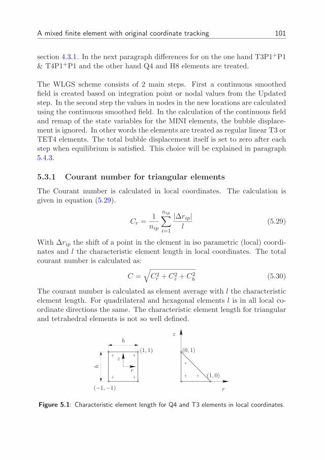
A mixed finite element with original coordinate tracking 101
section 4.3.1. In the next paragraph differences for on the one hand T3P1+P1& T4P1+P1 and the other hand Q4 and H8 elements are treated.
The WLGS scheme consists of 2 main steps. First a continuous smoothedfield is created based on integration point or nodal values from the Updatedstep. In the second step the values in nodes in the new locations are calculatedusing the continuous smoothed field. In the calculation of the continuous fieldand remap of the state variables for the MINI elements, the bubble displace-ment is ignored. In other words the elements are treated as regular linear T3 orTET4 elements. The total bubble displacement itself is set to zero after eachstep when equilibrium is satisfied. This choice will be explained in paragraph5.4.3.
5.3.1 Courant number for triangular elements
The Courant number is calculated in local coordinates. The calculation isgiven in equation (5.29).
Cr =1
nip
nip∑
i=1
|∆rip|l
(5.29)
With ∆rip the shift of a point in the element in iso parametric (local) coordi-nates and l the characteristic element length in local coordinates. The totalcourant number is calculated as:
C =√
C2r + C2
z + C2h (5.30)
The courant number is calculated as element average with l the characteristicelement length. For quadrilateral and hexagonal elements l is in all local co-ordinate directions the same. The characteristic element length for triangularand tetrahedral elements is not so well defined.
h
h
(−1,−1)
(1, 1) (0, 1)
(1, 0)
r
r
z
z
Figure 5.1: Characteristic element length for Q4 and T3 elements in local coordinates.
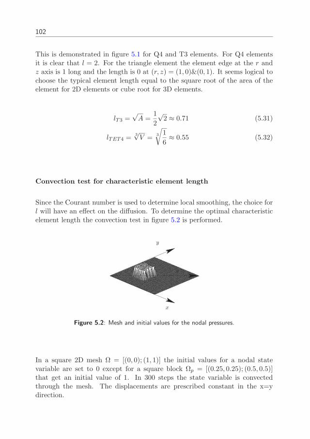
102
This is demonstrated in figure 5.1 for Q4 and T3 elements. For Q4 elementsit is clear that l = 2. For the triangle element the element edge at the r andz axis is 1 long and the length is 0 at (r, z) = (1, 0)&(0, 1). It seems logical tochoose the typical element length equal to the square root of the area of theelement for 2D elements or cube root for 3D elements.
lT3 =√
A =1
2
√2 ≈ 0.71 (5.31)
lTET4 =3√
V =3
√
1
6≈ 0.55 (5.32)
Convection test for characteristic element length
Since the Courant number is used to determine local smoothing, the choice forl will have an effect on the diffusion. To determine the optimal characteristicelement length the convection test in figure 5.2 is performed.
x
y
v
Figure 5.2: Mesh and initial values for the nodal pressures.
In a square 2D mesh Ω = [(0, 0); (1, 1)] the initial values for a nodal statevariable are set to 0 except for a square block Ωp = [(0.25, 0.25); (0.5, 0.5)]that get an initial value of 1. In 300 steps the state variable is convectedthrough the mesh. The displacements are prescribed constant in the x=ydirection.
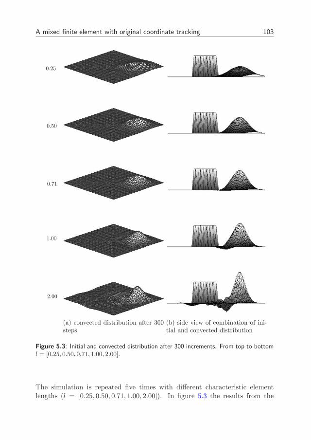
A mixed finite element with original coordinate tracking 103
0.25
0.50
0.71
1.00
2.00
(a) convected distribution after 300steps
(b) side view of combination of ini-tial and convected distribution
Figure 5.3: Initial and convected distribution after 300 increments. From top to bottoml = [0.25, 0.50, 0.71, 1.00, 2.00].
The simulation is repeated five times with different characteristic elementlengths (l = [0.25, 0.50, 0.71, 1.00, 2.00]). In figure 5.3 the results from the
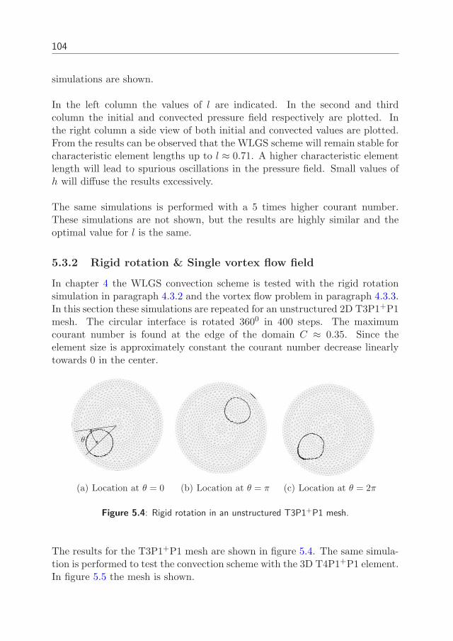
104
simulations are shown.
In the left column the values of l are indicated. In the second and thirdcolumn the initial and convected pressure field respectively are plotted. Inthe right column a side view of both initial and convected values are plotted.From the results can be observed that the WLGS scheme will remain stable forcharacteristic element lengths up to l ≈ 0.71. A higher characteristic elementlength will lead to spurious oscillations in the pressure field. Small values ofh will diffuse the results excessively.
The same simulations is performed with a 5 times higher courant number.These simulations are not shown, but the results are highly similar and theoptimal value for l is the same.
5.3.2 Rigid rotation & Single vortex flow field
In chapter 4 the WLGS convection scheme is tested with the rigid rotationsimulation in paragraph 4.3.2 and the vortex flow problem in paragraph 4.3.3.In this section these simulations are repeated for an unstructured 2D T3P1+P1mesh. The circular interface is rotated 3600 in 400 steps. The maximumcourant number is found at the edge of the domain C ≈ 0.35. Since theelement size is approximately constant the courant number decrease linearlytowards 0 in the center.
θ
(a) Location at θ = 0 (b) Location at θ = π (c) Location at θ = 2π
Figure 5.4: Rigid rotation in an unstructured T3P1+P1 mesh.
The results for the T3P1+P1 mesh are shown in figure 5.4. The same simula-tion is performed to test the convection scheme with the 3D T4P1+P1 element.In figure 5.5 the mesh is shown.
A mixed finite element with original coordinate tracking 105
Figure 5.5: Mesh for convection test in an unstructured T4P1+P1 mesh.
The results are shown in figure 5.6
(a) Location at θ = 0 (b) Location at θ = π (c) Location at θ = 2π
Figure 5.6: Rigid rotation in an unstructured T4P1+P1 mesh.
The overall result for this course mesh is very good. From these simulationscan be observed that in this linear prescribed displacement field some diffusionis introduced through the WLGS scheme.
Vortex flow
The vortex flow problem described in chapter 4 is repeated for unstructuredtriangular meshes. The velocity field is prescribed in rectangular domain of
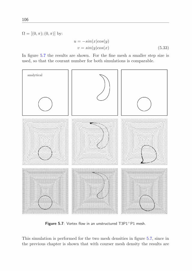
106
Ω = [(0, π); (0, π)] by:
u = −sin(x)cos(y)
v = sin(y)cos(x) (5.33)
In figure 5.7 the results are shown. For the fine mesh a smaller step size isused, so that the courant number for both simulations is comparable.
analytical
Figure 5.7: Vortex flow in an unstructured T3P1+P1 mesh.
This simulation is performed for the two mesh densities in figure 5.7, since inthe previous chapter is shown that with courser mesh density the results are
A mixed finite element with original coordinate tracking 107
not in good agreement with the analytical solution.
From the results of this simulation can be concluded that even for highlyinhomogeneous displacements fields the convection of the field is reasonable.The deviation in the final shape is caused by diffusive effects. This effect re-duces when less local smoothing is applied, however then oscillations in thefield at the edges of the domain appear.
5.4 Implementation in DiekA
5.4.1 Incremental-iterative update
In the previous section the main equations for the FEM discretisation arederived. In this section some extra implementation aspects are treated. Theseaspects are specific for these type of elements.
Integration The T3P1+P1 element is integrated using 3 integration pointsand the T4P1+P1 is integrated using 4 integration points.
5.4.2 Updated Lagrangian
The total stress is decomposed into a deviator and a hydrostatic part. Thedeviatoric stresses are stored as integration point values while the hydrostaticpressure are stored as nodal values. The total stress in an integration point inthe element can be written as:
σip = s + I∑
i
Mipi (5.34)
In the corrector step only the deviatoric stress is updated and the total stressis calculated using the new deviatoric stresses and the pressures from the so-lution from the predictor step, as in equation (5.34).
The calculation of the Jacobian matrix is performed without the bubble nodedisplacements. Omitting the bubble node displacements makes the Jacobianequal for all integration points.
The bubble degrees of freedom can be condensed on element level. This wouldreduce calculation time in the predictor step. However, the determinationof the bubble displacements for calculating the stresses in the corrector stepwould take more time. Here is chosen not to condense the bubble degrees offreedom.
108
5.4.3 Implementation for ALE
In the ALE step all the integration point variables and nodal variables haveto be convected to the new grid location. For the total pressures and lineardisplacements this is performed as described in the previous section. This alsomeans that the total bubble displacements are not known after convection.This has an impact on the calculation of the residual on the pressures.
Calculation of residual on pressure
From equation (5.26) can be found that the residual on the pressure Rp con-sists of the total displacements and total pressures at the beginning of the step.The calculation of the correct total bubble displacements after convection isnot a straight forward procedure.
Rp = R0p + ∆Rp + ∆Rc
p (5.35)
Rp =1
Cb
(p0 + ∆p + ∆pc) − 1 : B(u0 + ∆u + ∆uc) (5.36)
For an Updated Lagrangian simulation ∆u and ∆p are known and of course∆uc = 0 and ∆pc = 0. For an ALE simulation incremental values of the con-vective part are added. The convective increment of the linear displacementsand pressures is calculated. To get accurate results, the bubble displacementshave to be calculated correctly. Calculation of the convective part of the bub-ble proves to be difficult and results are poor.
Several methods to calculate the residual on the pressure have been inves-tigated in this research . The extrusion force for the simulation as in para-graph 5.6 is used to compare the results. In all options the calculation ofthe convective bubble increment is treated differently from the calculation ofthe convective linear displacement increment. Therefore equation (5.36) isrewritten as:
Rp =1
Cb
(p0 + ∆p + ∆pc) − 1 : B
(
u0 + ∆u +
∆ucl
∆ucb
)
(5.37)
To calculate the residual on the pressure different options are described below.

A mixed finite element with original coordinate tracking 109
0 0.02 0.04 0.06 0.08
11
10
12
13
14
15
0.10
Extr
usi
onfo
rce
[kN
/m
m]
Ram displacement [mm]
UL ∆RUL R
ALE ∆RALE Rtot
Figure 5.8: Extrusion force for residual on pressure.
The first option is to calculate a residual a zero convective contribution forthe bubble displacements in the remap of the variables:
Rp =1
Cb
(p0 + ∆p + ∆pc) − 1 : B
(
u0 + ∆u +
∆ucl
0
)
(5.38)
The total bubble displacement before and after remap are the same. Sincethe equilibrium is checked after convection in our semi-coupled approach, theequilibrium is still fulfilled. This option is depicted in figure 5.8 as R. Forthis option the updated simulation is unchanged. The ALE simulation showsa strong decay of the force over time. This decay is also found in the pressurein the container.
The second option is to convect the linear displacements and pressures. Thenbased on these values the bubble displacements that minimizes the ”con-vected” residual is calculated.
RALEp =
1
Cb
(p0 + ∆p + ∆pc) − 1 : B
(
u0 + ∆u +
∆ucl
∆uminb
)
(5.39)
The optimal convective bubble displacement is calculated by least squares fit-ting. This option shows an improvement in force decay with respect to the
110
previous option, however the results are still not in good agreement with theexpected values. The results for this option are not shown in the figure.
The third option is to ignore the residual on the pressures from the previousstep by setting R0
p = 0. The residual on the pressures is now only calcu-lated based on the incremental displacements and pressures. The total bubbledisplacement is set to zero at the beginning of each step.
RALEp =
1
Cb
(∆p + ∆pc) − 1 : B
(
∆u +
∆ucl
0
)
(5.40)
Within an iteration the updated incremental bubble displacement is also usedas convected incremental bubble displacement. This option is depicted in thefigure as ∆R. This option shows the proper force displacement curves for bothUpdated and ALE simulations.
From the previous results can be concluded that in both UL and ALE theresidual on the pressure from the previous step can be omitted. This optionis implemented in DiekA.
With this implementation the calculation of the total nodal bubble displace-ments ub can be ignored completely. At the end of every increment ub is setto zero.
Ru = F −∫
VBT
σ0dV (5.41)
Rp = 1Cb
(∆p + ∆pc) − 1 : B(∆u + ∆uc) (5.42)
5.5 Updated Lagrangian application: Tube expan-
sion
A long tube is loaded with an internal pressure p. The axial displacement issuppressed, making it a plane strain situation. The material model for thetube is chosen elastic rigid plastic.
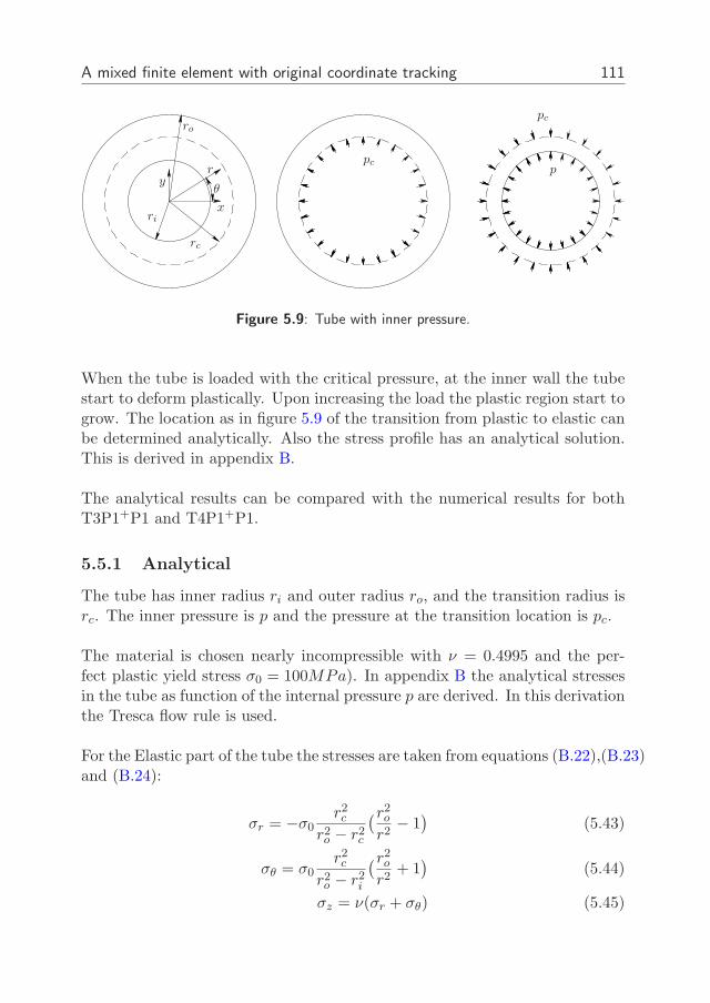
A mixed finite element with original coordinate tracking 111
rc
ri
ro
p
x
y
pc
pc
r
θ
Figure 5.9: Tube with inner pressure.
When the tube is loaded with the critical pressure, at the inner wall the tubestart to deform plastically. Upon increasing the load the plastic region start togrow. The location as in figure 5.9 of the transition from plastic to elastic canbe determined analytically. Also the stress profile has an analytical solution.This is derived in appendix B.
The analytical results can be compared with the numerical results for bothT3P1+P1 and T4P1+P1.
5.5.1 Analytical
The tube has inner radius ri and outer radius ro, and the transition radius isrc. The inner pressure is p and the pressure at the transition location is pc.
The material is chosen nearly incompressible with ν = 0.4995 and the per-fect plastic yield stress σ0 = 100MPa). In appendix B the analytical stressesin the tube as function of the internal pressure p are derived. In this derivationthe Tresca flow rule is used.
For the Elastic part of the tube the stresses are taken from equations (B.22),(B.23)and (B.24):
σr = −σ0r2c
r2o − r2
c
(r2o
r2− 1)
(5.43)
σθ = σ0r2c
r2o − r2
i
(r2o
r2+ 1)
(5.44)
σz = ν(σr + σθ) (5.45)
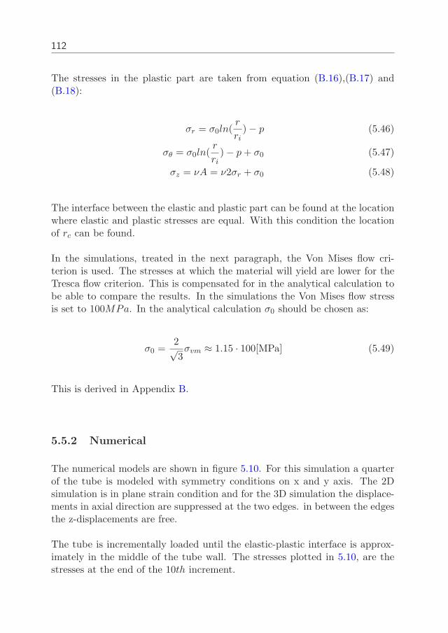
112
The stresses in the plastic part are taken from equation (B.16),(B.17) and(B.18):
σr = σ0ln(r
ri) − p (5.46)
σθ = σ0ln(r
ri) − p + σ0 (5.47)
σz = νA = ν2σr + σ0 (5.48)
The interface between the elastic and plastic part can be found at the locationwhere elastic and plastic stresses are equal. With this condition the locationof rc can be found.
In the simulations, treated in the next paragraph, the Von Mises flow cri-terion is used. The stresses at which the material will yield are lower for theTresca flow criterion. This is compensated for in the analytical calculation tobe able to compare the results. In the simulations the Von Mises flow stressis set to 100MPa. In the analytical calculation σ0 should be chosen as:
σ0 =2√3σvm ≈ 1.15 · 100[MPa] (5.49)
This is derived in Appendix B.
5.5.2 Numerical
The numerical models are shown in figure 5.10. For this simulation a quarterof the tube is modeled with symmetry conditions on x and y axis. The 2Dsimulation is in plane strain condition and for the 3D simulation the displace-ments in axial direction are suppressed at the two edges. in between the edgesthe z-displacements are free.
The tube is incrementally loaded until the elastic-plastic interface is approx-imately in the middle of the tube wall. The stresses plotted in 5.10, are thestresses at the end of the 10th increment.
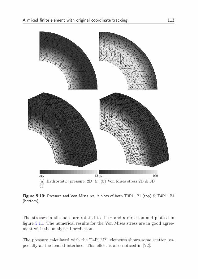
A mixed finite element with original coordinate tracking 113
12-35
(a) Hydrostatic pressure 2D &3D
10055
(b) Von Mises stress 2D & 3D
Figure 5.10: Pressure and Von Mises result plots of both T3P1+P1 (top) & T4P1+P1(bottom).
The stresses in all nodes are rotated to the r and θ direction and plotted infigure 5.11. The numerical results for the Von Mises stress are in good agree-ment with the analytical prediction.
The pressure calculated with the T4P1+P1 elements shows some scatter, es-pecially at the loaded interface. This effect is also noticed in [22].
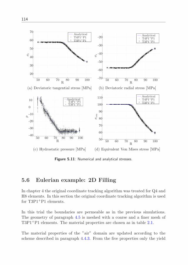
114
20
30
40
50
50
60
60
70
70 80 90 100
[mm]
AnalyticalT4P1+P1T3P1+P1
R
σt
(a) Deviatoric tangential stress [MPa]
50 60 70 80 90 100
-20
-30
-40
-50
-60
-70
AnalyticalT4P1+P1T3P1+P1
R
σr
(b) Deviatoric radial stress [MPa]
10
50 60 70 80 90 100
147
0
-10
-20
-30
-40
AnalyticalT4P1+P1T3P1+P1
R
p
(c) Hydrostatic pressure [MPa]
5050
60
60
70
70
80
80
90
90
100
100
110 AnalyticalT4P1+P1T3P1+P1
R
σvm
(d) Equivalent Von Mises stress [MPa]
Figure 5.11: Numerical and analytical stresses.
5.6 Eulerian example: 2D Filling
In chapter 4 the original coordinate tracking algorithm was treated for Q4 andH8 elements. In this section the original coordinate tracking algorithm is usedfor T3P1+P1 elements.
In this trial the boundaries are permeable as in the previous simulations.The geometry of paragraph 4.5 is meshed with a coarse and a finer mesh ofT3P1+P1 elements. The material properties are chosen as in table 2.1.
The material properties of the ”air” domain are updated according to thescheme described in paragraph 4.4.3. From the five properties only the yield
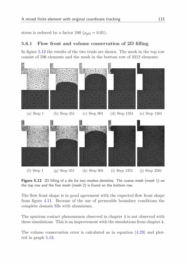
A mixed finite element with original coordinate tracking 115
stress is reduced by a factor 100 (ρyld = 0.01).
5.6.1 Flow front and volume conservation of 2D filling
In figure 5.12 the results of the two trials are shown. The mesh in the top rowconsist of 596 elements and the mesh in the bottom row of 2212 elements.
(a) Step 1 (b) Step 451 (c) Step 901 (d) Step 1351 (e) Step 1501
(f) Step 1 (g) Step 451 (h) Step 901 (i) Step 1351 (j) Step 2501
Figure 5.12: 2D filling of a die for two meshes densities. The coarse mesh (mesh 1) onthe top row and the fine mesh (mesh 2) is found on the bottom row.
The flow front shape is in good agreement with the expected flow front shapefrom figure 4.11. Because of the use of permeable boundary conditions thecomplete domain fills with aluminium.
The spurious contact phenomenon observed in chapter 4 is not observed withthese simulations. This is an improvement with the simulations from chapter 4.
The volume conservation error is calculated as in equation (4.23) and plot-ted in graph 5.13.
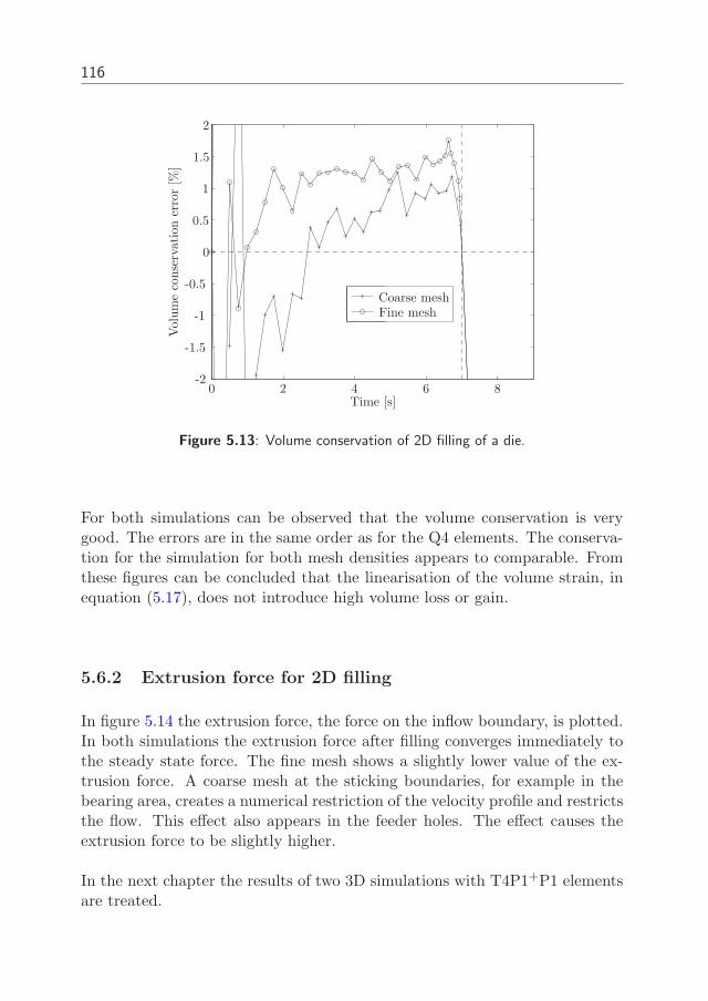
116
0
0
0.5
1
2
2 4 6 8
1.5
-1.5
-2
-1
-0.5
Vol
um
eco
nse
rvati
on
erro
r[%
]
Time [s]
Coarse meshFine mesh
Figure 5.13: Volume conservation of 2D filling of a die.
For both simulations can be observed that the volume conservation is verygood. The errors are in the same order as for the Q4 elements. The conserva-tion for the simulation for both mesh densities appears to comparable. Fromthese figures can be concluded that the linearisation of the volume strain, inequation (5.17), does not introduce high volume loss or gain.
5.6.2 Extrusion force for 2D filling
In figure 5.14 the extrusion force, the force on the inflow boundary, is plotted.In both simulations the extrusion force after filling converges immediately tothe steady state force. The fine mesh shows a slightly lower value of the ex-trusion force. A coarse mesh at the sticking boundaries, for example in thebearing area, creates a numerical restriction of the velocity profile and restrictsthe flow. This effect also appears in the feeder holes. The effect causes theextrusion force to be slightly higher.
In the next chapter the results of two 3D simulations with T4P1+P1 elementsare treated.
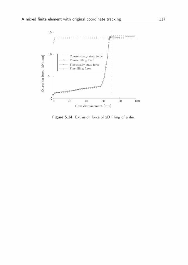
A mixed finite element with original coordinate tracking 117
0 20 40 60 80 100
5
15
10
Extr
usi
onfo
rce
[kN
/m
m]
Ram displacement [mm]
Coarse steady state force
Coarse filling force
Fine steady state force
Fine filling force
Figure 5.14: Extrusion force of 2D filling of a die.

118
Chapter 6
Two applications
In this chapter two applications with the MINI elements combined with theoriginal coordinate tracking algorithm are considered. The elements and track-ing algorithm are implemented in the implicit FEM code DiekA. From bothexamples the experimental results are known and treated in previous chapters.
From the first simulation it is shown that the T4P1+P1 elements give goodresults for a large number of increments. The second simulation is an im-provement of the 3D filling simulation from chapter 4. In this chapter thesimulation is performed using T4P1+P1 elements. Since automatic meshingwith T4P1+P1 elements is available, it is easier to add detail to the simu-lation. The other reason for using T4P1+P1 elements is the spurious effectsfound with filling with H8 elements.
The last part of the filling simulation is the forming of the nose piece. Tobe able to model this nose piece, the use of special ALE options is treated.
6.1 Container flow
In chapter 3 front lines in container flow (figure 6.1) during rod extrusionwere created based on steady state numerical results and compared with ex-periments.
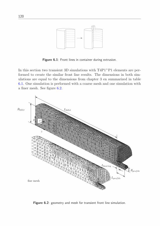
120
Figure 6.1: Front lines in container during extrusion.
In this section two transient 3D simulations with T4P1+P1 elements are per-formed to create the similar front line results. The dimensions in both sim-ulations are equal to the dimensions from chapter 3 en summarized in table6.1. One simulation is performed with a coarse mesh and one simulation witha finer mesh. See figure 6.2.
y x
z
Rbillet
Rprofile
Lbillet
Lprofile
Lbearing
fine mesh
Figure 6.2: geometry and mesh for transient front line simulation.
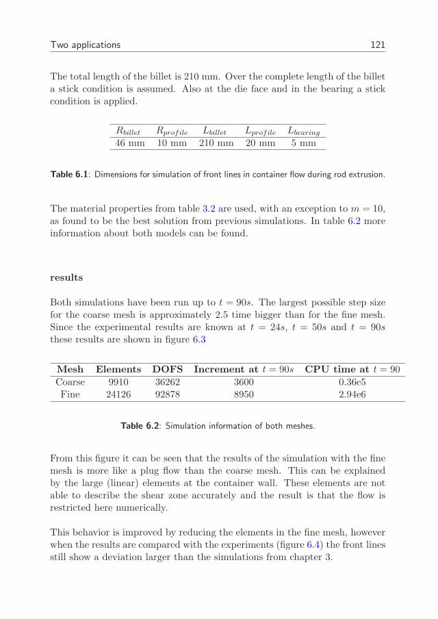
Two applications 121
The total length of the billet is 210 mm. Over the complete length of the billeta stick condition is assumed. Also at the die face and in the bearing a stickcondition is applied.
Rbillet Rprofile Lbillet Lprofile Lbearing
46 mm 10 mm 210 mm 20 mm 5 mm
Table 6.1: Dimensions for simulation of front lines in container flow during rod extrusion.
The material properties from table 3.2 are used, with an exception to m = 10,as found to be the best solution from previous simulations. In table 6.2 moreinformation about both models can be found.
results
Both simulations have been run up to t = 90s. The largest possible step sizefor the coarse mesh is approximately 2.5 time bigger than for the fine mesh.Since the experimental results are known at t = 24s, t = 50s and t = 90s
these results are shown in figure 6.3
Mesh Elements DOFS Increment at t = 90s CPU time at t = 90
Coarse 9910 36262 3600 0.36e5Fine 24126 92878 8950 2.94e6
Table 6.2: Simulation information of both meshes.
From this figure it can be seen that the results of the simulation with the finemesh is more like a plug flow than the coarse mesh. This can be explainedby the large (linear) elements at the container wall. These elements are notable to describe the shear zone accurately and the result is that the flow isrestricted here numerically.
This behavior is improved by reducing the elements in the fine mesh, howeverwhen the results are compared with the experiments (figure 6.4) the front linesstill show a deviation larger than the simulations from chapter 3.
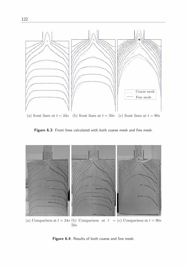
122
(a) front lines at t = 24s (b) front lines at t = 50s
Coarse mesh
Fine mesh
(c) front lines at t = 90s
Figure 6.3: Front lines calculated with both coarse mesh and fine mesh.
(a) Comparison at t = 24s (b) Comparison at t =50s
(c) Comparison at t = 90s
Figure 6.4: Results of both coarse and fine mesh.
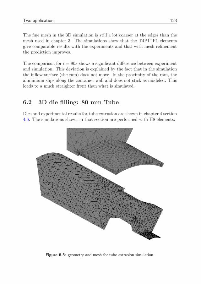
Two applications 123
The fine mesh in the 3D simulation is still a lot coarser at the edges than themesh used in chapter 3. The simulations show that the T4P1+P1 elementsgive comparable results with the experiments and that with mesh refinementthe prediction improves.
The comparison for t = 90s shows a significant difference between experimentand simulation. This deviation is explained by the fact that in the simulationthe inflow surface (the ram) does not move. In the proximity of the ram, thealuminium slips along the container wall and does not stick as modeled. Thisleads to a much straighter front than what is simulated.
6.2 3D die filling: 80 mm Tube
Dies and experimental results for tube extrusion are shown in chapter 4 section4.6. The simulations shown in that section are performed with H8 elements.
Figure 6.5: geometry and mesh for tube extrusion simulation.
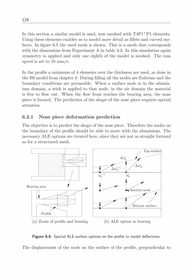
124
In this section a similar model is used, now meshed with T4P1+P1 elements.Using these elements enables us to model more detail as fillets and curved sur-faces. In figure 6.5 the used mesh is shown. This is a mesh that correspondswith the dimensions from Experiment A in table 4.3. In this simulation againsymmetry is applied and only one eighth of the model is meshed. The ramspeed is set to 10 mm/s.
In the profile a minimum of 4 elements over the thickness are used, as done inthe H8 model from chapter 4. During filling all the nodes are Eulerian and theboundary conditions are permeable. When a surface node is in the alumin-ium domain, a stick is applied to that node, in the air domain the materialis free to flow out. When the flow front reaches the bearing area, the nosepiece is formed. The prediction of the shape of the nose piece requires specialattention
6.2.1 Nose piece deformation prediction
The objective is to predict the shape of the nose piece. Therefore the nodes onthe boundary of the profile should be able to move with the aluminium. Thenecessary ALE options are treated here, since they are not as straight forwardas for a structured mesh.
Bearing area
Profile
(a) Zoom of profile and bearing
∆ui−1m
∆uim
∆uig
ui−10 ui
0
Top surface
Bottom surface
Interior node
(b) ALE option in bearing
Figure 6.6: Special ALE surface options on the profile to model deflections.
The displacement of the node on the surface of the profile, perpendicular to
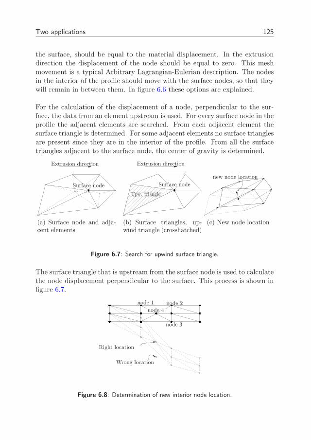
Two applications 125
the surface, should be equal to the material displacement. In the extrusiondirection the displacement of the node should be equal to zero. This meshmovement is a typical Arbitrary Lagrangian-Eulerian description. The nodesin the interior of the profile should move with the surface nodes, so that theywill remain in between them. In figure 6.6 these options are explained.
For the calculation of the displacement of a node, perpendicular to the sur-face, the data from an element upstream is used. For every surface node in theprofile the adjacent elements are searched. From each adjacent element thesurface triangle is determined. For some adjacent elements no surface trianglesare present since they are in the interior of the profile. From all the surfacetriangles adjacent to the surface node, the center of gravity is determined.
Extrusion direction
Surface node
(a) Surface node and adja-cent elements
Upw. triangle
Extrusion direction
Surface node
(b) Surface triangles, up-wind triangle (crosshatched)
new node location
(c) New node location
Figure 6.7: Search for upwind surface triangle.
The surface triangle that is upstream from the surface node is used to calculatethe node displacement perpendicular to the surface. This process is shown infigure 6.7.
node 1 node 2
node 3
node 4
Wrong location
Right location
Figure 6.8: Determination of new interior node location.
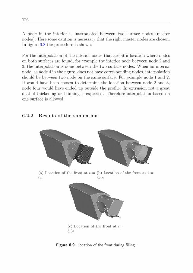
126
A node in the interior is interpolated between two surface nodes (masternodes). Here some caution is necessary that the right master nodes are chosen.In figure 6.8 the procedure is shown.
For the interpolation of the interior nodes that are at a location where nodeson both surfaces are found, for example the interior node between node 2 and3, the interpolation is done between the two surface nodes. When an interiornode, as node 4 in the figure, does not have corresponding nodes, interpolationshould be between two node on the same surface. For example node 1 and 2.If would have been chosen to determine the location between node 2 and 3,node four would have ended up outside the profile. In extrusion not a greatdeal of thickening or thinning is expected. Therefore interpolation based onone surface is allowed.
6.2.2 Results of the simulation
(a) Location of the front at t =0s
(b) Location of the front at t =3.4s
(c) Location of the front at t =5.3s
Figure 6.9: Location of the front during filling.
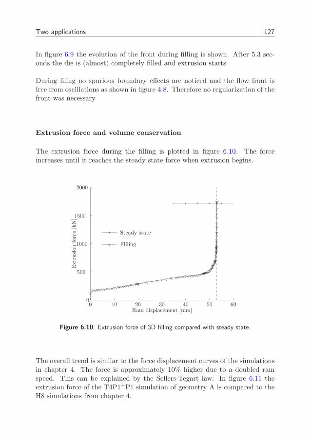
Two applications 127
In figure 6.9 the evolution of the front during filling is shown. After 5.3 sec-onds the die is (almost) completely filled and extrusion starts.
During filing no spurious boundary effects are noticed and the flow front isfree from oscillations as shown in figure 4.8. Therefore no regularization of thefront was necessary.
Extrusion force and volume conservation
The extrusion force during the filling is plotted in figure 6.10. The forceincreases until it reaches the steady state force when extrusion begins.
00 10 20 30 40 50 60
1500
2000
500
1000
Extr
usi
onfo
rce
[kN
]
Ram displacement [mm]
Steady state
Filling
Figure 6.10: Extrusion force of 3D filling compared with steady state.
The overall trend is similar to the force displacement curves of the simulationsin chapter 4. The force is approximately 10% higher due to a doubled ramspeed. This can be explained by the Sellers-Tegart law. In figure 6.11 theextrusion force of the T4P1+P1 simulation of geometry A is compared to theH8 simulations from chapter 4.
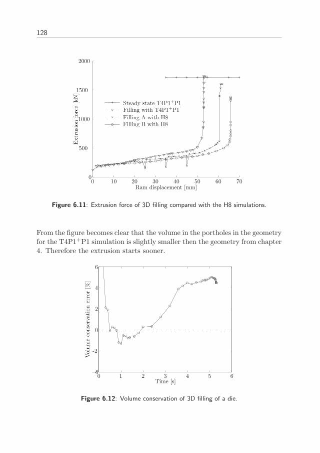
128
00 10 20 30 40 50 60 70
1500
2000
500
1000
Extr
usi
onfo
rce
[kN
]
Ram displacement [mm]
Steady state T4P1+P1Filling with T4P1+P1
Filling A with H8Filling B with H8
Figure 6.11: Extrusion force of 3D filling compared with the H8 simulations.
From the figure becomes clear that the volume in the portholes in the geometryfor the T4P1+P1 simulation is slightly smaller then the geometry from chapter4. Therefore the extrusion starts sooner.
−4
0
0 1
2
2 3
4
4 5
6
6
-2
Vol
um
eco
nse
rvat
ion
erro
r[%
]
Time [s]
Figure 6.12: Volume conservation of 3D filling of a die.
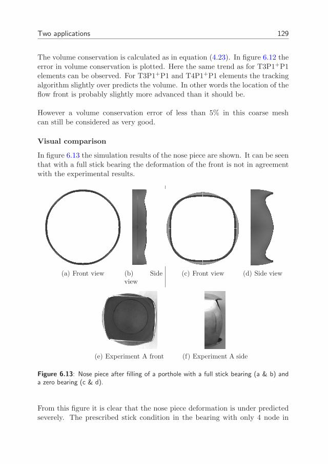
Two applications 129
The volume conservation is calculated as in equation (4.23). In figure 6.12 theerror in volume conservation is plotted. Here the same trend as for T3P1+P1elements can be observed. For T3P1+P1 and T4P1+P1 elements the trackingalgorithm slightly over predicts the volume. In other words the location of theflow front is probably slightly more advanced than it should be.
However a volume conservation error of less than 5% in this coarse meshcan still be considered as very good.
Visual comparison
In figure 6.13 the simulation results of the nose piece are shown. It can be seenthat with a full stick bearing the deformation of the front is not in agreementwith the experimental results.
(a) Front view (b) Sideview
(c) Front view (d) Side view
(e) Experiment A front (f) Experiment A side
Figure 6.13: Nose piece after filling of a porthole with a full stick bearing (a & b) anda zero bearing (c & d).
From this figure it is clear that the nose piece deformation is under predictedseverely. The prescribed stick condition in the bearing with only 4 node in
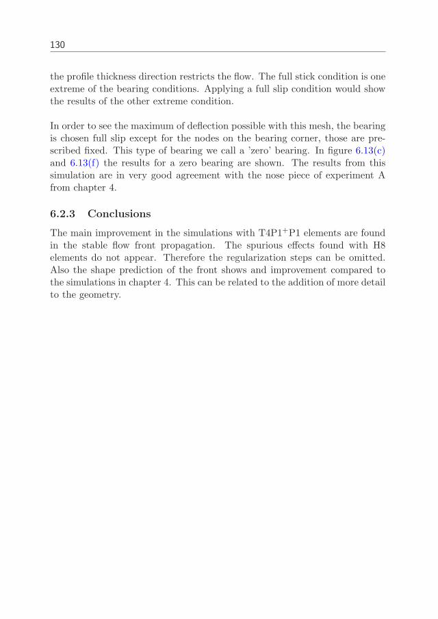
130
the profile thickness direction restricts the flow. The full stick condition is oneextreme of the bearing conditions. Applying a full slip condition would showthe results of the other extreme condition.
In order to see the maximum of deflection possible with this mesh, the bearingis chosen full slip except for the nodes on the bearing corner, those are pre-scribed fixed. This type of bearing we call a ’zero’ bearing. In figure 6.13(c)and 6.13(f) the results for a zero bearing are shown. The results from thissimulation are in very good agreement with the nose piece of experiment Afrom chapter 4.
6.2.3 Conclusions
The main improvement in the simulations with T4P1+P1 elements are foundin the stable flow front propagation. The spurious effects found with H8elements do not appear. Therefore the regularization steps can be omitted.Also the shape prediction of the front shows and improvement compared tothe simulations in chapter 4. This can be related to the addition of more detailto the geometry.
Chapter 7
Conclusions &
Recommendations
In this research numerical simulations of aluminium extrusion has been stud-ied. Especially simulation of the aluminium flow during the filling of the dieand creation of the nose piece has been treated.
In general can be said that most effects in extrusion can be qualitatively de-scribed by the simulations. Hence it can be said that these models profideinsight in the extrusion process. However quantitatively the results deviatefrom the experimental results.
The general conclusions for steady state simulations are:
In chapter 3 was shown that the velocity field from steady state sim-ulations can be accurately post-processed to the transient front lines.This method has been used as an inverse method to determine materialproperties under extrusion conditions.
The general conclusions for interface tracking simulations are:
The initial coordinate function is an appropriate function to track in-terfaces in two phase flows. In chapter 4 an ALE/Eulerian formulationwith initial coordinate interface tracking has been successfully used forthe simulation of the transient start-up of aluminium extrusion process.The initial coordinate tracking method shows good volume conservation.The trend in the prediction of the nose piece shape is in agreement withthe experiments. The quantitative distortions are under predicted.
132
An element from the MINI-family was successfully developed for a semi-coupled ALE formulation. The initial interface tracking algorithm workswell with the MINI element.
The spurious effects in the flow front prediction found with H8 elementsis not appearent in simulations with T4P1+P1 elements. Therefore alsothe regularisation can be omitted in filling simulations with T4P1+P1elements.Meshing with triangular or tetrahedral elements from the MINI-familyincreases the possibility to include details as radii. From the tube extru-sion simulation in chapter 6 can be concluded that increasing detail in-creases the quantitative agreement of the simulations with experiments.
Some general recommendations are:
In simulations in this thesis the dies are assumed rigid. It is well knownthat die deflection can play an important role in aluminium flow throughthe die, especially in the bearing area. Further research on die deflectioncan give useful insight for a better equivalent bearing model and betterunderstanding of stresses in the die during start-up and steady state.
The flow stress and other material properties of aluminium at extrusiontemperatures are sensitive for small differences. Thermo-mechanicallycoupled simulations will improve the quantitative agreement betweensimulations and experiments.
Material properties under extrusion temperatures are essential for ac-curate simulations. The development of a validated material propertiesdatabase and scatter analysis of different alloys would be a helpful toolfor further developments in extrusion die design based on simulations.
The used regularisation of the original coordinate function is a diffu-sive step. Other and better regularisation techniques can be found inthe level set approaches. These better regularization techniques wouldimprove the accuracy and speed of the simulations.
The current state of developments in aluminium extrusion requires more ex-perimental validation of numerical results to increase quantitatively accuracy.In this thesis two methods have been presented to compare experiments withnumerical results. These methods help to improve material models and togain insight in aluminium flow during start-up.
Appendix A
Weak formulation
A.1 Isotropic Elasto plastic material
σ = E : ε − 2Gεpl (A.1)
To obtain objective integration the derivation of Lof [44] is closely followed.Lof chooses to use a corotational formulation. The initial deviatoric stress σ
is replaced by σ:
σ = RσRT (A.2)
Where R follows from the polar decomposition of the incremental deformationgradient F. From the differentiation of this equation with respect to timefollows the Jaumann stress rate
O
σ= 2G(I − 1
311) : D − 3G
(1 + h)σ2y
ss : D + Cb11 : D − σtrD (A.3)
O
σ= Y : D + Cb11 : D − σtrD (A.4)
A.2 Strong formulation
σn+1 · ∇ = 0 in Ωn+1
g
u = un+10 on Γu
σn+1 · n = tn+1 on Γt
(A.5)
134
A.3 Weak formulation
In the finite element formulation the equilibrium equations are only weaklyenforced. This weak form is equal to the virtual power equation if the weighingfunctions w is equal to the virtual velocity δv. When bodyforces are neglected,the so-called weak form can be written as:
δWin = δWext (A.6)∫
Ωn+1
(w
∇) : σn+1 dΩ =
∫
Γn+1
w · tn+1 dΓt (A.7)
Since the material model is given as the mateerial rate of the stress-strainrelation, the rate or the weak form is used. The increase in virtual work fromΩn at tn to Ωn+1 at tn+1 can be approximated by:
δWn+1in ≈ δWn
in + δWin ∆t (A.8)
δWn+1ext ≈ δWn
ext + δWext ∆t (A.9)
from whitch the updated lagrangian formulation can be derived:
δWin = δWext (A.10)
Using [42] and [72] the derivation for the rate of weak form is given. The firststep is to translate the weak form A.7 into referential coordinates.
∫
Ωχ
∂w
∂χ
∂χ
∂x: σJχ dΩχ =
∫
Γχ
w · tJΓ dΓχ (A.11)
with the surface Jacobian JΓ and:
Jχ = det
(
∂x
∂χ
)
(A.12)
Using the following definitions for the deformation gradient F and the velocitygradient L:
F =∂x
∂χ(A.13)
L = v
∇ (A.14)
The velocity gradient L can be decomposed into a symmetric part and anskew-symmetric part:
L = D + W (A.15)
Weak formulation 135
With the symmetric part D and the skew-symmetricpart W:
D =1
2
(
v
∇ +
∇v)
(A.16)
W =1
2
(
v
∇ −
∇v)
(A.17)
δWin =
∫
Ωχ
∂w
∂χ:(
F−1 · σJχ + F−1 · σJχ + F−1 · σJχ
)
dΩχ (A.18)
The rates of the weighing functions vanish [29]. The three time derivativesare:
F−1 = −F−1L (A.19)
Jχ = Jχtr (L) (A.20)
σ =∇σ −σ · W + W · σ (A.21)
Substitution and transforming back to the spatial coordinates gives:
δWin =
∫
Ωw
∇:(
− L · σ + σ + σtrL)
dΩ (A.22)
The virtual external work written in referential coordinates:
δWext =
∫
Γt
w · t dΓt =
∫
Γχ
w · tJS dΓχ =
∫
Γχ
w · σ · nJΓ dΓχ (A.23)
The time derivative of the virtual work is:
δWext =
∫
Γχ
w ·(
σJΓ + σJΓ)
· ndΓχ (A.24)
Transforming back the the spatial coordinates using σ · n = t gives:
δWext =
∫
Γt
w · t dΓt +
∫
Γt
w · tJΓ dΓt (A.25)
The complete weak form can now be written as:∫
Ωw
∇:(
− L · σ + σ + σtrL)
dΩ =
∫
Γt
w · t dΓt +
∫
Γt
w · tJΓ dΓt (A.26)

136

Appendix B
Stresses in a long cylinder
under internal pressure
In this appendix the stresses for an elastic-perfect plastic tube under innnerpressure are derived. The derivation closely follows the solution from Pettersson[52].
rc
ri
ro
p
x
y
pc
pc
r
θ
Figure B.1: Vortex flow for triangles
The stresses are derived with a plane strain condition and with the use of thetresca flow criterion.
138
The stress-strain relations are
εr =1
E(σr − ν(σz + σθ)) + εp
r (B.1)
εθ =1
E(σθ − ν(σz + σr)) + ε
pθ (B.2)
εz =1
E(σz − ν(σr + σθ)) + εp
z (B.3)
From equilibrium in radial direction can be derived:
dσr
dr=
σθ − σr
r(B.4)
And the compatibility equation
dεθ
dr=
εr − εθ
r(B.5)
In a elastic region εz = 0 and εpz = 0. (B.3) can be rewrtitten into:
σz = ν(σr + σθ) (B.6)
Combining equations (B.2),(B.3),(B.4) and (B.6) leads to:
dσθ
dr= −dσr
dror (B.7)
σθ = −σr + A (B.8)
This combined with (B.4) yields
dσr
dr+
2σr
r=
A
r(B.9)
Equation (B.9) together with the boundary conditions σr(ri) = −p, σr(ro) = 0give for the elastic case:
σr = −pr2i
r2o − r2
i
(r2o
r2− 1)
(B.10)
σθ = pr2i
r2o − r2
i
(r2o
r2+ 1)
(B.11)
σz = 2pνr2i
r2o − r2
i
(B.12)
Stresses in a long cylinder under internal pressure 139
For the plastic part Tresca’s flow hypothesis σθ − σr = σ0 is used. This is canbe substituted in (B.4) and integrated.
dσr
dr=
σ0
r(B.13)
σr = σ0ln(r) + B (B.14)
With the boundary condition σr = −p at r = ri
σr = σ0ln(r
ri) − p (B.15)
This can be substituted in tresca’s flow rule to get σθ. The complete set ofstresses for the plastic part is written as:
σr = σ0ln(r
ri) − p (B.16)
σθ = σ0ln(r
ri) − p + σ0 (B.17)
σz = ν(σr + σθ) (B.18)
With rc the radius of the interface between plastic and elastic, and pc = −σr‖rc
the pressure at the interface the equations for the elastic part can be given.Using
σr = −pcr2c
r2o − r2
c
(r2o
r2− 1)
(B.19)
σθ = pcr2c
r2o − r2
i
(r2o
r2+ 1)
(B.20)
σz = ν(σr + σθ) (B.21)
With these formulas it is possible to determine pc = σ0.
σr = −σ0r2c
r2o − r2
c
(r2o
r2− 1)
(B.22)
σθ = σ0r2c
r2o − r2
i
(r2o
r2+ 1)
(B.23)
σz = ν(σr + σθ) (B.24)
The simulations in chapter 5 use a Von Mises flow criterion. The Von Misesflow criterion for this problem is written as:
σvm =√
σ2r + σ2
z + σ2θ − σrσθ − σrσz − σzσθ (B.25)
140
σz = ν(σr + σθ) and this can be substituted in the Von Mises flow criterion.
σvm =√
σ2r + ν2(σr + σθ)2 + σ2
θ − σrσθ − σrν(σr + σθ) − ν(σr + σθ)σθ (B.26)
Since the material is nearly incompressible ν = 0.4995 ≈ 0.5 the Von Misesflow criterion can be simplified.
σvm =1
2
√3√
σ2r + σ2
θ − 2σrσθ = (B.27)
1
2
√3√
(σr − σθ)2 (B.28)
And this can be related to the Tresca flow criterion as in equation (B.30).
σvm =1
2
√3√
(σr − σθ)2 =1
2
√3σ0 (B.29)
In the simulations the use yield stress is 100Mpa. To be able to compareresults with analytical values, σ0 should be chosen as:
σ0 =2√3σvm ≈ 1.15 · 100[MPa] (B.30)
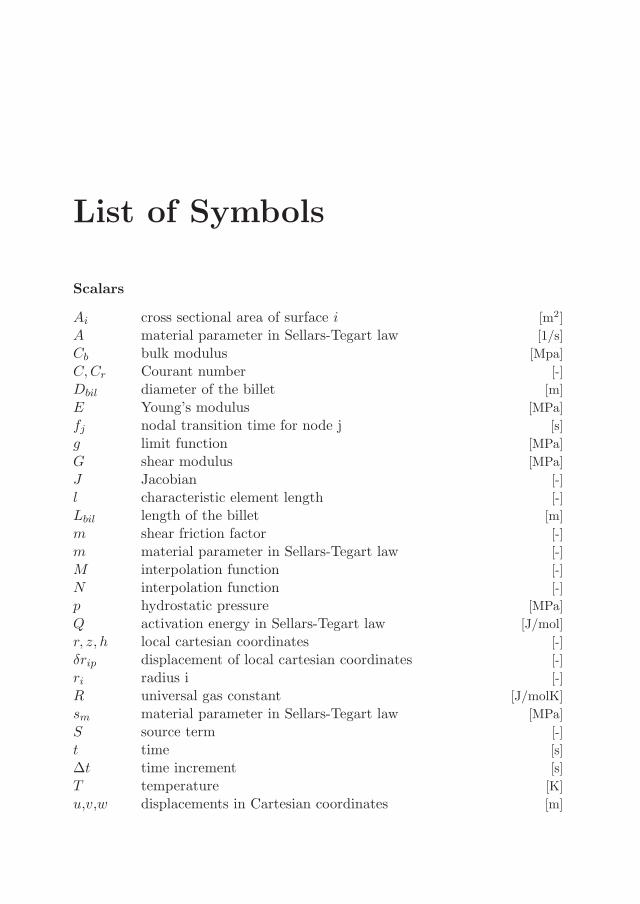
List of Symbols
Scalars
Ai cross sectional area of surface i [m2]
A material parameter in Sellars-Tegart law [1/s]
Cb bulk modulus [Mpa]
C, Cr Courant number [-]
Dbil diameter of the billet [m]
E Young’s modulus [MPa]
fj nodal transition time for node j [s]
g limit function [MPa]
G shear modulus [MPa]
J Jacobian [-]
l characteristic element length [-]
Lbil length of the billet [m]
m shear friction factor [-]
m material parameter in Sellars-Tegart law [-]
M interpolation function [-]
N interpolation function [-]
p hydrostatic pressure [MPa]
Q activation energy in Sellars-Tegart law [J/mol]
r, z, h local cartesian coordinates [-]
δrip displacement of local cartesian coordinates [-]
ri radius i [-]
R universal gas constant [J/molK]
sm material parameter in Sellars-Tegart law [MPa]
S source term [-]
t time [s]
∆t time increment [s]
T temperature [K]
u,v,w displacements in Cartesian coordinates [m]
142
wi weighing function for node i [-]
W work [J]
x, y, z Cartesian coordinates [m]
X0 original coordinate [m]
X current coordinate [m]
α weight factor for global smoothing,upwind parameter [-]
β, βr local smoothing parameter [-]
∆λ plastic multiplier [1/MPa]
εr radial strain component [-]
Γ surface [-]
Γf location of initial front line [-]
κ equivalent plastic strain [-]
κ0 parameter to include elastic region in Sellars-Tegart law [1/s]
µ friction coefficient [-]
ν Poisson ratio [-]
Ω domain [-]
ϕ normal angle in bearing [o]
φ concentration function [-]
ρyld multipication factor for pseudo material [-]
σy yield stress [MPa]
σr radial stress component [MPa]
σ effective stress [MPa]
θ angle [o]
ξ state variable [-]
Vectors
f nodal transition times [s]
Fint internal force vector [N ]
Fext external force vector [N ]
n normal [-]
Ri residual force vector of the ith iteration [N ]
t traction forces [N/m2]
ug nodal grid displacements [m]
um nodal material displacements [m]
uc nodal convective displacements [m]
∆ug incremental nodal grid displacements [m]
∆um incremental nodal material displacements [m]
∆uc incremental nodal convective displacements [m]
vg nodal grid velocities [m/s]
List of Symbols 143
vm nodal material velocities [m/s]
vc nodal convective velocities [m/s]
w weighing function [-]
x Spatial coordinate [m]
X0 original coordinate [m]
X current coordine [m]
Tensors
B tensor relating D to v [1/m]
D rate of deformation [1/s]
ε small deformation strain [-]
∆ε total strain increment [-]
∆εe elastic strain increment [-]
∆εvp (visco)plastic strain increment [-]
E elastic tensor [MPa]
∆e deviatoric strain increment [-]
F deformation gradient [-]
I 4th order unity tensor [-]
1 2th order unity tensor [-]
Lg grid velocity gradient [1/s]
L material velocity gradient [1/s]
σ Chauchy stress [MPa]
∆σ stress increment [MPa]O
σ corotational stress rate [MPa/s]
s deviatoric stress [MPa]
W Spin tensor [1/s]
Y Yield tensor [MPa]
Matrices
K tangential stiffness matrix [N/m]
Abbreviations
ALE Arbitrary Lagrangian EulerianCPU Central Processing UnitDG Discontinuous GalerkinDMZ Dead Metal Zone

144
DOF Degree Of FreedomDOFS Degrees Of FreedomER Extrusion RatioFEM Finite Element MethodSUPG Stream Upwind Petrov GalerkinWLGS Weighted Local and Global Smoothing
Miscellaneous
∇x Gradient of scalar gives vector∇x Gradient of vector gives tensor∇ · x =divx
Divergence of vector gives scalar
x time derivative of x
xT transpose of x
trx trace of x
Bibliography
[1] Proceedings of Eight International Aluminium Extrusion Technology Seminar.In Eight International Aluminium Extrusion Technology Seminar, Florida, 2004.
[2] proceedings of Extrusion Bologna. In Extrusion Bologna, Bologna, 2007.
[3] R. Akeret and W. Strehmel. Control of metal flow in extrusion dies. In Fourth
International Aluminum Extrusion Technology Seminar, 1988.
[4] D.N. Arnold, F. Brezzi, and M. Fortin. A stable finite element for the Stokesequations. Calcolo, 21(4):337–344, 1984.
[5] W. Assaad, H.J.M. Geijselaers, and J. Huetink. Boundary conditions applied onbearing corner in direct aluminum extrusion, 2009.
[6] N. Biba, A. Vlasov, and S. Stebounov. The simulation of the extrusion processusing QForm3D. In Latest advances in extrusion technology in Europa and second
extrusion benchmark, Bologna, 2007.
[7] F. Brezzi. On the existence, uniqueness and approximation of saddle-point prob-lems arising from Lagrangian multipliers. RAIRO Anal. Numer., 8:129–151,1974.
[8] D. Brokken. Numerical modelling of ductile fracture in blanking. PhD thesis,Eindhoven University of Technology, 1999.
[9] A.N. Brooks and T.J.R. Hughes. Streamline upwind/Petrov-Galerkin formula-tions for convection dominated flows with particular emphasis on the incom-pressible Navier-Stokes equations. Computer Methods in Applied Mechanics and
Engineering, 32(1-3):199, 1982.
[10] T. Chanda, J. Zhou, and J. Duszczyk. A comparative study on iso-speed ex-trusion and isothermal extrusion of AA6061 alloy using 3D FEM simulation.Journal of Materials Processing Technology, 114(2):145–153, 2001.
[11] A.J. Chorin. A numerical method for solving incompressible viscous flow prob-lems. Journal of Computational Physics, 2(1):12–26, 1967.
[12] C. Devals, M. Heniche, F. Bertrand, R.E. Hayes, and P.A. Tanguy. A finiteelement strategy for the solution of interface tracking problems. International
Journal for Numerical Methods in Fluids, 49(12):1305–1327, 2005.
145
146
[13] L. Donati and L. Tomesani. Seam welds modeling and mechanical propertiesprediction in the extrusion of AA6082 alloy. In Latest advances in extrusion
technology in Europa and second extrusion benchmark, Bologna, 2007.
[14] L. Donati, L. Tomesani, and V. Giacomelli. Evaluation Of A New FEM Cri-terion For Seam Welds Quality Prediction In Aluminum Extruded Profiles. InProceedings of the eight international alumnium extrusion technology seminar,volume II, pages 221–234, 2004.
[15] J. Donea. Taylor-Galerkin method for convective transport problems. Interna-
tional Journal for Numerical Methods in Engineering, 20(1):101–119, 1984.
[16] J. Donea, S. Giuliani, and J.P. Halleux. An arbitrary lagrangian-eulerian finiteelement method for transient dynamic fluid-structure interactions. Computer
Methods in Applied Mechanics and Engineering, 33(1-3):689, 1982.
[17] E.N. Dvorkin, M.A. Cavaliere, and M.B. Goldschmit. A three field element viaAugmented Lagrangian for modelling bulk metal forming processes. Computa-
tional Mechanics, 17(1-2):2–9, 1995.
[18] E.N. Dvorkin and E.G. Petocz. An effective technique for moddeling 2D metalforming processes using an eulerian technique. Engineering Computations,10(4):323–336, 1993.
[19] I. Flitta and T. Sheppard. Temperature Changes and their Effect on Deformationduring Extrusion using FEM. In Proceedings of the eight international alumnium
extrusion technology seminar, volume I, pages 269–283, 2004.
[20] J.M. Floryan and H. Rasmussen. Numerical methods for viscous flows withmoving boundaries. Appl. Mech. Rev., 42(12):323–341, 1989.
[21] M. Fortin and A. Fortin. A new approach for the FEM simulation of viscoelasticflows. Journal of Non-Newtonian Fluid Mechanics, 32(3):295–310, 1989.
[22] C. Gay, P. Montmitonnet, T. Coupez, and J.L. Chenot. Test of an elementsuitable for fully automatic remeshing in 3D elastoplastic simulation of coldforging. J. Mater. Process. Technol, 45:683–688, 1994.
[23] H.J.M Geijselaers. Numerical simulations of stresses due to solid state transfor-
mations. PhD thesis, University of Twente, 2003.
[24] D. Greaves. Simulation of interface and free surface flows in a viscous fluid usingadapting quadtree grids. International Journal for Numerical Methods in Fluids,44(10):1093, 2004.
[25] F. Halvorsen and T. Aukrust. Studies of the Effects of Flow Imbalance on ShapeVariations in Aluminum Extrusion by use of Lagrangian FEM Software. InProceedings of the eight international alumnium extrusion technology seminar,volume I, pages 243–251, 2004.
[26] L.R. Herrmann. Elasticity equations for incompressible, or nearly incompressiblematerials by a variational principle theorem. AIAA, 3(10):1896–1900, 1965.
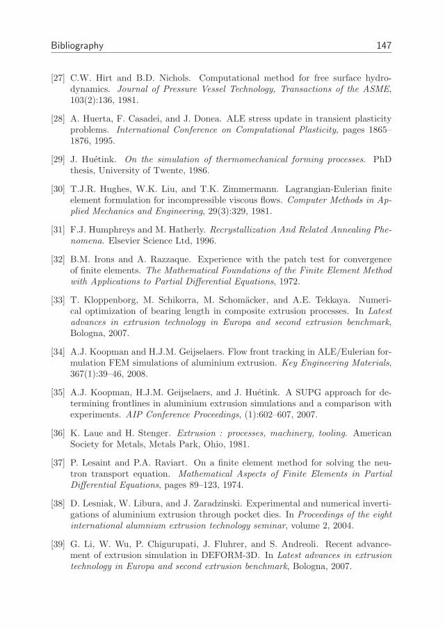
Bibliography 147
[27] C.W. Hirt and B.D. Nichols. Computational method for free surface hydro-dynamics. Journal of Pressure Vessel Technology, Transactions of the ASME,103(2):136, 1981.
[28] A. Huerta, F. Casadei, and J. Donea. ALE stress update in transient plasticityproblems. International Conference on Computational Plasticity, pages 1865–1876, 1995.
[29] J. Huetink. On the simulation of thermomechanical forming processes. PhDthesis, University of Twente, 1986.
[30] T.J.R. Hughes, W.K. Liu, and T.K. Zimmermann. Lagrangian-Eulerian finiteelement formulation for incompressible viscous flows. Computer Methods in Ap-
plied Mechanics and Engineering, 29(3):329, 1981.
[31] F.J. Humphreys and M. Hatherly. Recrystallization And Related Annealing Phe-
nomena. Elsevier Science Ltd, 1996.
[32] B.M. Irons and A. Razzaque. Experience with the patch test for convergenceof finite elements. The Mathematical Foundations of the Finite Element Method
with Applications to Partial Differential Equations, 1972.
[33] T. Kloppenborg, M. Schikorra, M. Schomacker, and A.E. Tekkaya. Numeri-cal optimization of bearing length in composite extrusion processes. In Latest
advances in extrusion technology in Europa and second extrusion benchmark,Bologna, 2007.
[34] A.J. Koopman and H.J.M. Geijselaers. Flow front tracking in ALE/Eulerian for-mulation FEM simulations of aluminium extrusion. Key Engineering Materials,367(1):39–46, 2008.
[35] A.J. Koopman, H.J.M. Geijselaers, and J. Huetink. A SUPG approach for de-termining frontlines in aluminium extrusion simulations and a comparison withexperiments. AIP Conference Proceedings, (1):602–607, 2007.
[36] K. Laue and H. Stenger. Extrusion : processes, machinery, tooling. AmericanSociety for Metals, Metals Park, Ohio, 1981.
[37] P. Lesaint and P.A. Raviart. On a finite element method for solving the neu-tron transport equation. Mathematical Aspects of Finite Elements in Partial
Differential Equations, pages 89–123, 1974.
[38] D. Lesniak, W. Libura, and J. Zaradzinski. Experimental and numerical inverti-gations of aluminium extrusion through pocket dies. In Proceedings of the eight
international alumnium extrusion technology seminar, volume 2, 2004.
[39] G. Li, W. Wu, P. Chigurupati, J. Fluhrer, and S. Andreoli. Recent advance-ment of extrusion simulation in DEFORM-3D. In Latest advances in extrusion
technology in Europa and second extrusion benchmark, Bologna, 2007.
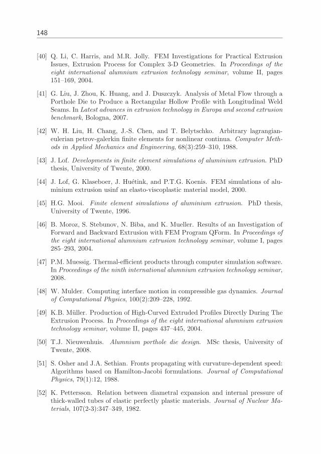
148
[40] Q. Li, C. Harris, and M.R. Jolly. FEM Investigations for Practical ExtrusionIssues, Extrusion Process for Complex 3-D Geometries. In Proceedings of the
eight international alumnium extrusion technology seminar, volume II, pages151–169, 2004.
[41] G. Liu, J. Zhou, K. Huang, and J. Duszczyk. Analysis of Metal Flow through aPorthole Die to Produce a Rectangular Hollow Profile with Longitudinal WeldSeams. In Latest advances in extrusion technology in Europa and second extrusion
benchmark, Bologna, 2007.
[42] W. H. Liu, H. Chang, J.-S. Chen, and T. Belytschko. Arbitrary lagrangian-eulerian petrov-galerkin finite elements for nonlinear continua. Computer Meth-
ods in Applied Mechanics and Engineering, 68(3):259–310, 1988.
[43] J. Lof. Developments in finite element simulations of aluminium extrusion. PhDthesis, University of Twente, 2000.
[44] J. Lof, G. Klaseboer, J. Huetink, and P.T.G. Koenis. FEM simulations of alu-minium extrusion usinf an elasto-viscoplastic material model, 2000.
[45] H.G. Mooi. Finite element simulations of aluminium extrusion. PhD thesis,University of Twente, 1996.
[46] B. Moroz, S. Stebunov, N. Biba, and K. Mueller. Results of an Investigation ofForward and Backward Extrusion with FEM Program QForm. In Proceedings of
the eight international alumnium extrusion technology seminar, volume I, pages285–293, 2004.
[47] P.M. Muessig. Thermal-efficient products through computer simulation software.In Proceedings of the ninth international alumnium extrusion technology seminar,2008.
[48] W. Mulder. Computing interface motion in compressible gas dynamics. Journal
of Computational Physics, 100(2):209–228, 1992.
[49] K.B. Muller. Production of High-Curved Extruded Profiles Directly During TheExtrusion Process. In Proceedings of the eight international alumnium extrusion
technology seminar, volume II, pages 437–445, 2004.
[50] T.J. Nieuwenhuis. Alumnium porthole die design. MSc thesis, University ofTwente, 2008.
[51] S. Osher and J.A. Sethian. Fronts propagating with curvature-dependent speed:Algorithms based on Hamilton-Jacobi formulations. Journal of Computational
Physics, 79(1):12, 1988.
[52] K. Pettersson. Relation between diametral expansion and internal pressure ofthick-walled tubes of elastic perfectly plastic materials. Journal of Nuclear Ma-
terials, 107(2-3):347–349, 1982.
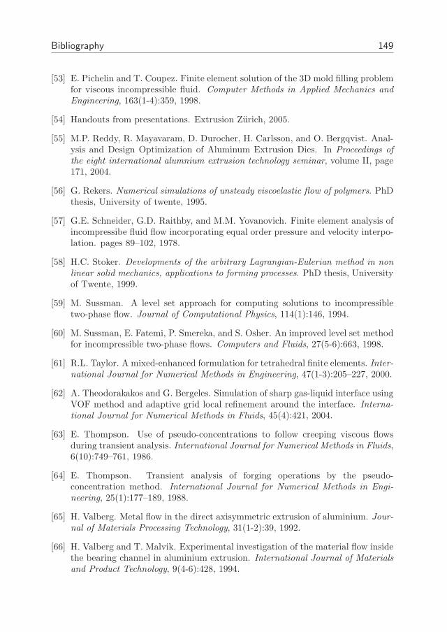
Bibliography 149
[53] E. Pichelin and T. Coupez. Finite element solution of the 3D mold filling problemfor viscous incompressible fluid. Computer Methods in Applied Mechanics and
Engineering, 163(1-4):359, 1998.
[54] Handouts from presentations. Extrusion Zurich, 2005.
[55] M.P. Reddy, R. Mayavaram, D. Durocher, H. Carlsson, and O. Bergqvist. Anal-ysis and Design Optimization of Aluminum Extrusion Dies. In Proceedings of
the eight international alumnium extrusion technology seminar, volume II, page171, 2004.
[56] G. Rekers. Numerical simulations of unsteady viscoelastic flow of polymers. PhDthesis, University of twente, 1995.
[57] G.E. Schneider, G.D. Raithby, and M.M. Yovanovich. Finite element analysis ofincompressibe fluid flow incorporating equal order pressure and velocity interpo-lation. pages 89–102, 1978.
[58] H.C. Stoker. Developments of the arbitrary Lagrangian-Eulerian method in non
linear solid mechanics, applications to forming processes. PhD thesis, Universityof Twente, 1999.
[59] M. Sussman. A level set approach for computing solutions to incompressibletwo-phase flow. Journal of Computational Physics, 114(1):146, 1994.
[60] M. Sussman, E. Fatemi, P. Smereka, and S. Osher. An improved level set methodfor incompressible two-phase flows. Computers and Fluids, 27(5-6):663, 1998.
[61] R.L. Taylor. A mixed-enhanced formulation for tetrahedral finite elements. Inter-
national Journal for Numerical Methods in Engineering, 47(1-3):205–227, 2000.
[62] A. Theodorakakos and G. Bergeles. Simulation of sharp gas-liquid interface usingVOF method and adaptive grid local refinement around the interface. Interna-
tional Journal for Numerical Methods in Fluids, 45(4):421, 2004.
[63] E. Thompson. Use of pseudo-concentrations to follow creeping viscous flowsduring transient analysis. International Journal for Numerical Methods in Fluids,6(10):749–761, 1986.
[64] E. Thompson. Transient analysis of forging operations by the pseudo-concentration method. International Journal for Numerical Methods in Engi-
neering, 25(1):177–189, 1988.
[65] H. Valberg. Metal flow in the direct axisymmetric extrusion of aluminium. Jour-
nal of Materials Processing Technology, 31(1-2):39, 1992.
[66] H. Valberg and T. Malvik. Experimental investigation of the material flow insidethe bearing channel in aluminium extrusion. International Journal of Materials
and Product Technology, 9(4-6):428, 1994.
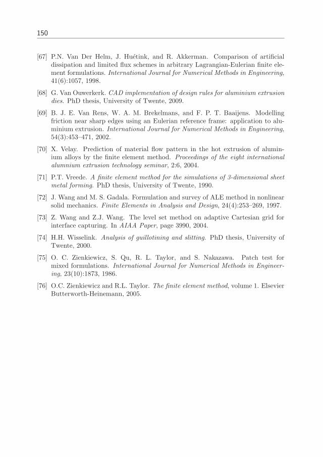
150
[67] P.N. Van Der Helm, J. Huetink, and R. Akkerman. Comparison of artificialdissipation and limited flux schemes in arbitrary Lagrangian-Eulerian finite ele-ment formulations. International Journal for Numerical Methods in Engineering,41(6):1057, 1998.
[68] G. Van Ouwerkerk. CAD implementation of design rules for aluminium extrusion
dies. PhD thesis, University of Twente, 2009.
[69] B. J. E. Van Rens, W. A. M. Brekelmans, and F. P. T. Baaijens. Modellingfriction near sharp edges using an Eulerian reference frame: application to alu-minium extrusion. International Journal for Numerical Methods in Engineering,54(3):453–471, 2002.
[70] X. Velay. Prediction of material flow pattern in the hot extrusion of alumin-ium alloys by the finite element method. Proceedings of the eight international
alumnium extrusion technology seminar, 2:6, 2004.
[71] P.T. Vreede. A finite element method for the simulations of 3-dimensional sheet
metal forming. PhD thesis, University of Twente, 1990.
[72] J. Wang and M. S. Gadala. Formulation and survey of ALE method in nonlinearsolid mechanics. Finite Elements in Analysis and Design, 24(4):253–269, 1997.
[73] Z. Wang and Z.J. Wang. The level set method on adaptive Cartesian grid forinterface capturing. In AIAA Paper, page 3990, 2004.
[74] H.H. Wisselink. Analysis of guillotining and slitting. PhD thesis, University ofTwente, 2000.
[75] O. C. Zienkiewicz, S. Qu, R. L. Taylor, and S. Nakazawa. Patch test formixed formulations. International Journal for Numerical Methods in Engineer-
ing, 23(10):1873, 1986.
[76] O.C. Zienkiewicz and R.L. Taylor. The finite element method, volume 1. ElsevierButterworth-Heinemann, 2005.

Dankwoord
Een kort dankwoord is wel op zijn plaats na het afmaken van een proefschrift.Het voltooien van dit proefschrift is alleen geslaagd door de enorme inzet,bereidwilligheid en hulp van veel mensen. Ik kijk met veel dankbaarheid terugop de afgelopen jaren. Ik hoop dan ook dat ik niemand te kort doe in ditdankwoord en als dat wel het geval is, dan bied ik op voorhand mijn excusesaan.
Veel dank ben ik verschuldigd aan Prof. Dr. Ir. J. Huetink, mijn promotor.Beste Han, het begon met jouw uitnodiging om dit onderzoek te gaan doen enhet eindigt met dit boekje als resultaat. Het was niet altijd even makkelijk,maar ik heb me altijd gesteund en gemotiveerd gevoeld door alle gesprekken.Je liet me ook steeds weer versteld staan van je enorme kennis en inzicht,niet alleen van je eigen vakgebied maar ook ver daarbuiten. Daarnaast is joubetrokkenheid bij iedereen onder je hoede een geweldig voorbeeld.
Ik dank ook Dr. Ir. H.J.M. Geijselaers voor zijn begeleiding afgelopen jaren.Geijs, toen ik zeven jaar geleden afstudeerde, kwam promoveren kort tersprake. Jij sprak toen de woorden:”Dat is niets voor jou!”. Gelukkig wasik die woorden vergeten toen ik twee jaar later toch nog begon aan een pro-motieopdracht opdracht. Gedurende mijn promotie heb ik er regelmatig aangedacht, en je had gelijk. Gelukkig is het dankzij jou ondersteuning en hulptoch gelukt.
Ik wil ook Kjell Nilsen en Peter Koenis van Boalgroup bedanken voor hetfinancieel mogelijk maken van dit onderzoek en hun bijdrage aan het experi-menteel deel van mijn proefschrift. Gijs van Ouwerkerk wil ik als projectpart-ner bedanken voor het meedenken aan oplossingen en het gezelschap naar deconferenties. Onze muzieksmaak loopt uiteen, maar met de humor zitten weop een lijn. Als we moeten lachen, dan gieren we het uit.
152
Tanja en Debbie, ontzettend bedankt voor de gesprekjes en alle (last minute)regelwerk dat jullie voor ons promovendi doen. Bovendien vrolijken jullie hetgeheel van stoffige wetenschappers flink op!
Ik wil ook alle collega’s waarmee ik afgelopen jaren heb gewerkt bedanken vooralle steun en gezelligheid. Lunchwandelaars, het was wat minder frequent deafgelopen tijd, maar ik hoop dat ik nog een paar jaar mee mag wandelen.Ekke, als we (twee-jaren-) plannen maken dan voeren we ze ook goed uit! Ikheb veel van je geleerd en ik hoop dat je weet hoe dankbaar ik ben dat ik jouheb leren kennen. Ook dank ik de studenten die aan dit onderzoek hebbenmeegewerkt. Johan, Bastiaan, Kees Durk en Thijs. Het was goed om jullieals klankbord en hulp te mogen hebben.
De laatsten zullen de eersten zijn. Lieve ouders en zus, heel erg bedanktvoor jullie steun, klushulp bij verhuizen, financiele steun bij krapte en onvoor-waardelijke liefde en begrip als ik weer aan het werk moest en niet veel tijdmaakte om thuis mee te dragen.
Lieve Wilma, het viel niet mee he, afgelopen jaar met mij. Je had wel delasten, maar niet de lusten van ons kersverse huwelijk. Ik ben dankbaar datje het toch hebt aangedurfd om met me te trouwen zo vlak voor het einde vanmijn promotie. Naast al je liefde, ben ik je ook veel verschuldigd voor allezorgzaamheid thuis. Je bent echt een hulp voor mij geweest afgelopen jaar!
Bert Koopman, mei 2009