Algorithmique des couplages et cryptographie - Lix

Algorithmique des couplages et cryptographie

THESE

presentee et soutenue publiquement le 14 mai 2010

pour l’obtention du

Doctorat de l’universit e de Versailles Saint-Quentin-en-Yvelines(specialite informatique)

Sorina IONICA

Composition du jury

Jean-Marc Couveignes RapporteurLouis Goubin ExaminateurAntoine Joux Directeur de theseDavid Kohel RapporteurTanja Lange ExaminateurAriane Mezard ExaminateurBenjamin Smith Examinateur

3

Remerciements

Ce travail n’aurait probablement pas vu le jour sans l’aide et la direction de mes professeurs.Je remercie Antoine Joux, mon directeur de these, d’avoir guide mes pas vers le monde de larecherche. Il m’est tres difficile de le remercier en une seule phrase pour tout ce qu’il a su metransmettre. J’essaie quand meme :(( Les idees simples sont aussi les plus belles)).Je doisenormementa Ariane Mezard, pour les mathematiques que j’ai apprises d’elle, pour sonenthousiasme envers la recherche, pour ses encouragements. Mercia elle pour tout le temps qu’ellea investit dans cette these.

J’ai une pensee toute particuliere pour Marcel Tena, qui fut mon professeur de mathematiquesau lycee, et gracea qui j’ai decouvert l’algebre. J’espere, Monsieur le professeur, ne pas vous avoirtrop decu et que vous trouverez dans ces pages, malgre le grand nombre de lignes de pseudocode,des maths aussi belles que celles que vous m’aviez apprises.

Je tiensa remercier Louis Goubin et Michael Quisquater de m’avoir propose de travailler surle projet Secure Algorithm, ainsi que pour nos collaborations lors des enseignements. Merciames co-auteurs, Nadia El Mrabet et Nicolas Guillermin, ainsi qu’a Jean-Claude Bajard et SylvainDuquesne d’avoir suivi notre travail. Je remercie Tanja Lange pour la lecture de mes articles etpour ses remarques. Je suis reconnaisantea mes collegues qui ont lu et corrige des parties de cemanuscrit : Anja Becker, Peter Birkner, Nadia El Mrabet, Malika Izabachene, Bastien Vayssiere,Vanessa Vitse. Mercia Cris car sans son aide les courbes dans ma these ne seraient pas aussibelles !

Le tour des thesards maintenant, ou devrais-je dire le tour des cryptogirls... ? Mercia Aureliede m’avoir accueilliea mon arrive au laboratoire, d’avoir corrige les fautes d’orthographe de monrapport de stage. Je remercie Joana, ma co-bureau, pour son enthousiasme et sa bonne humeurhabituelle, pour avoir rempli le bureau de toutes les langues du monde (l’espagnol, l’allemand,le portugais, l’alsacien, le roumain et meme le francais). Je remercie Vanessa pour nos discus-sions qui m’ont fait me sentir moins seule (dans un monde cruellement envahipar les bases deGrobner), et aussi pour une certaine implementation que je n’aurais jamais eu le courage de faire.Mais, malgre les rumeurs, le Prism n’est pas uneecole de femmes. Mercia Jean-Michel de faireface,a Sebastien de m’avoir fait rire (et pleurer) tant de fois ! Un grand mercia Stephane, le(( res-ponsable)) Linux de toutes mes machines, pour sa disponibilite permanente ainsi que pour avoireu une reponsea toute question. Mercia tous les(( archi)) que j’ai eu l’occasion de croiser.Ce que je garderai vifa l’esprit ? Les Tds en L1 soigneusement rediges avec des stylos Barbie, lescadeaux d’Aurelie pour le 1er mars, les photos de Thierry (mercia Thierry pour les perruques), larump session d’Eurocrypt, la poudre de craie cachee sous le bureau de L., les pamplemousses deSeb, les histoires de Stephane...

Merci a mes amis d’ici et de tres loin pour leur soutien permanent, sans lequel je ne seraispeut etre pas arrivee au bout de ce chemin. Mercia Miru, Iuli et toute la bande de faire mesretoursa Bucarest plus beaux, de me rappeler constamment d’ou je viens. Mercia Adi de m’avoirencourageea partir et finir mesetudesa l’etranger.Quanta ceux d’ici, merci de m’avoir adoptee,a Villeneuve-sur-Lot, au sein d’une bande de futursingenieurs un peu fous (born in Regie). Le temps s’estecoule tres vite : au campus gris de l’X, enpassant apres par la rue de Tolbiac, ou je trainais plus de temps que chez moi, pour arriver enfinala maison de Chantiers, toujours tres animee (je n’oublierai pas la musique !). Mercia eux d’avoirfait de Paris ma deuxieme maison. DistrusX rulz !

Mes derniers mots sont pour ma famille,a Bucarest eta Craiova. Je leur remercie pour leursoutien inconditionnel tout au long de mes annees d’etudes. Qu’ils sachent que, malgre ces mo-ments d’absence, je pense forta eux.

5

A mes grandparentsBunicilor mei

Table des matieres

1 Introduction 111.1 Couplages et cryptographie . . . . . . . . . . . . . . . . . . . . . . . . . . . .. 121.2 Motivation des travaux et objectifs de la these . . . . . . . . . . . . . . . . . . . 141.3 Contributions et organisation de cette these . . . . . . . . . . . . . . . . . . . . 16

I Preliminaries 19

2 Arithmetic of elliptic curves 212.1 Algebraic varieties . . . . . . . . . . . . . . . . . . . . . . . . . . . . . . . . . 212.2 Algebraic curves . . . . . . . . . . . . . . . . . . . . . . . . . . . . . . . . . . 252.3 Divisors . . . . . . . . . . . . . . . . . . . . . . . . . . . . . . . . . . . . . . . 272.4 Elliptic curves and Weierstrass equations . . . . . . . . . . . . . . . . . . . . .. 292.5 The Group Law . . . . . . . . . . . . . . . . . . . . . . . . . . . . . . . . . . . 302.6 Isogenies . . . . . . . . . . . . . . . . . . . . . . . . . . . . . . . . . . . . . . 312.7 Endomorphisms and automorphisms of an elliptic curve . . . . . . . . . . . . . . 352.8 Twists of elliptic curves . . . . . . . . . . . . . . . . . . . . . . . . . . . . . . . 352.9 The Weil pairing . . . . . . . . . . . . . . . . . . . . . . . . . . . . . . . . . . 362.10 The Tate pairing . . . . . . . . . . . . . . . . . . . . . . . . . . . . . . . . . . . 37

3 Complex Multiplication 393.1 Orders in quadratic imaginary fields . . . . . . . . . . . . . . . . . . . . . . . . 393.2 Lattices overC and the Weierstrass℘-function . . . . . . . . . . . . . . . . . . . 423.3 The j-invariant and the class equation . . . . . . . . . . . . . . . . . . . . . . . 443.4 The j-function and the modular equation . . . . . . . . . . . . . . . . . . . . . . 453.5 Elliptic curves overC . . . . . . . . . . . . . . . . . . . . . . . . . . . . . . . . 473.6 Elliptic curves over finite fields . . . . . . . . . . . . . . . . . . . . . . . . . . . 48

3.6.1 Hasse’s theorem and the endomorphism ring . . . . . . . . . . . . . . . 483.6.2 Reduction and lifting of curves . . . . . . . . . . . . . . . . . . . . . . . 493.6.3 Modular polynomials over finite fields . . . . . . . . . . . . . . . . . . . 50

4 Computational preliminaries 534.1 Miller’s algorithm . . . . . . . . . . . . . . . . . . . . . . . . . . . . . . . . . . 534.2 The Complex Multiplication Method for Elliptic Curves . . . . . . . . . . . . . 54

7

8

4.3 A method to construct curves with almost prime group order . . . . . . . . . .. 554.4 The Cocks-Pinch method . . . . . . . . . . . . . . . . . . . . . . . . . . . . . . 574.5 Velu’s formulae . . . . . . . . . . . . . . . . . . . . . . . . . . . . . . . . . . . 584.6 Counting the number of points on an elliptic curve . . . . . . . . . . . . . . . . 60

II Pairings and Isogeny Volcanoes 63

5 Isogeny Volcanoes 655.1 Isogeny volcanoes . . . . . . . . . . . . . . . . . . . . . . . . . . . . . . . . . .655.2 The modular polynomial approach . . . . . . . . . . . . . . . . . . . . . . . . . 68

5.2.1 Using modular polynomials to travel on volcanoes . . . . . . . . . . . . 685.2.2 Walking the volcano . . . . . . . . . . . . . . . . . . . . . . . . . . . . 68

5.3 Our approach . . . . . . . . . . . . . . . . . . . . . . . . . . . . . . . . . . . . 705.3.1 The group structure of the elliptic curve on the volcano . . . . . . . . . . 705.3.2 Preliminary results. Determining directions on the volcano . . . . . . . . 745.3.3 Numeric examples . . . . . . . . . . . . . . . . . . . . . . . . . . . . . 805.3.4 Walking on the volcano: new algorithms . . . . . . . . . . . . . . . . . . 81

5.4 Complexities and efficiency comparison . . . . . . . . . . . . . . . . . . . . . . 825.4.1 Irregular volcanoes . . . . . . . . . . . . . . . . . . . . . . . . . . . . . 865.4.2 Practical examples . . . . . . . . . . . . . . . . . . . . . . . . . . . . . 86

5.5 Two volcano-based algorithms . . . . . . . . . . . . . . . . . . . . . . . . . . . 885.5.1 Computing the Hilbert polynomial via isogeny volcanoes . . . . . . . . . 885.5.2 Modular polynomials via isogeny volcanoes . . . . . . . . . . . . . . . . 89

5.6 Conclusion . . . . . . . . . . . . . . . . . . . . . . . . . . . . . . . . . . . . . 90

III Pairings and Cryptography 91

6 Efficient Implementation of Cryptographic Pairings 936.1 Pairings in cryptography . . . . . . . . . . . . . . . . . . . . . . . . . . . . . . 936.2 Formulas for pairing computation . . . . . . . . . . . . . . . . . . . . . . . . . 95

6.2.1 The Case of Curves with Even Embedding Degree . . . . . . . . . . . . 976.3 Self-pairings and distortion maps . . . . . . . . . . . . . . . . . . . . . . . . . . 1006.4 Constructing non-degenerate self-pairings on ordinary curves . .. . . . . . . . . 1016.5 Speeding up pairing computation using isogenies . . . . . . . . . . . . . . . . .1036.6 Computational costs . . . . . . . . . . . . . . . . . . . . . . . . . . . . . . . . . 1066.7 Conclusion . . . . . . . . . . . . . . . . . . . . . . . . . . . . . . . . . . . . . 107

7 Pairings on Edwards curves 1097.1 Edwards curves . . . . . . . . . . . . . . . . . . . . . . . . . . . . . . . . . . . 1097.2 Pairing computation in Edwards coordinates . . . . . . . . . . . . . . . . . . . .111

7.2.1 An isogeny of degree 4 . . . . . . . . . . . . . . . . . . . . . . . . . . . 1127.2.2 Miller’s algorithm on the Edwards curve . . . . . . . . . . . . . . . . . . 1147.2.3 Pairing computation in Edwards coordinates . . . . . . . . . . . . . . . 114

9

7.3 A recent approach to pairing computation in Edwards coordinates . . . .. . . . 1197.4 An algorithm for scalar multiplication on incomplete Edwards curves . . . . . .1207.5 Future work. Computing the Ate pairing on Edwards curves . . . . . . . . .. . 1237.6 Conclusion . . . . . . . . . . . . . . . . . . . . . . . . . . . . . . . . . . . . . 124

8 Conclusion 1258.1 Limitations of our methods and open problems . . . . . . . . . . . . . . . . . . 126

Chapitre 1

Introduction

En cryptographie moderne, nous distinguons deux principales techniques de chiffrement. Laplus ancienne est la cryptographie symetrique, ou encorea cle secrete, qui repose sur le prin-cipe que deux parties doivent detenir un secret commun pour pouvoirechanger de l’informationchiffree. La deuxieme, la cryptographie asymetrique, est parue en 1976, quand Diffie et Hell-man [30] proposent pour la premiere fois un schema de chiffrement ne necessitant pas la connais-sance prealable d’un meme secret. Aujourd’hui, dans un systeme securise, la cryptographiea clesecrete et cellea cle publique sont utilisees conjointement, afin d’offrir un chiffrement rapide del’information. Dans un premier temps, un schemaa cle publique est utilise pourechanger unecle commune secrete. Ensuite, cette cle secrete est utilisee pour securiser,a l’aide d’un schemasymetrique, la communication entre l’emetteur et le destinataire.

Nous decrivons le protocole d’echange de clef propose par Diffie et Hellman, pour un groupeabstraitG, note additivement, qui est engendre par unelementP. Deux parties Alice (A) et Bob(B) detiennent les parametres publics (G,+,P) et veulent se mettre d’accord sur une cle commune,qui est unelement du groupe. A choisita ∈ N et calculePA = aP, tandis queB choisitb ∈ N etcalculePB = bP. Ils echangent publiquement ces valeurs. Ayant recuPB, A calcule

Pk = aPB = abP.

De la meme maniere, B recoitPA et calcule

Pk = bPA = abP.

La securite de ce protocole repose sur la difficulte du probleme du logarithme discret dans legroupeG. Cette difficulte signifie qu’etant donne un pointP et xP, un multiple scalaire du pointP, il est calculatoirement difficile de retrouverx. La difficulte de ce probleme dependevidemmentdu choix du groupe (G,+). En effet, si le probleme du logarithme discretetait facile dans le groupeG, un attaquant Charlie, reussissanta intercepterPA ou PB, pourrait calculera ou b et retrouverPk.

Afin de pouvoir developper des cryptosystemes comme celui de Diffie et Hellman, il est doncindispensable de trouver des groupes dans lesquels le probleme du logarithme discret sembledifficile. Notons qu’il existe des attaques, dites generiques, qui fonctionnent dans tous les groupes.Les meilleures attaques generiques contre le logarithme discret sont les attaques de Shanks [85] etde Pollard [79]. Leur complexite estO(

√r), ou r est le plus grand facteur premier de la cardinalite

11

12

de la courbe. Diffie et Hellman [30] ont propose le groupe multiplicatif d’un corps fini. Neanmoins,dans ces groupes, il existe des methodes dites de ”calcul d’indice”, qui resolvent le probleme dulogarithme discret avec une complexite sous-exponentielle [52, 53]. Pour ameliorer la securite, lelogarithme discret sur les courbes elliptiques ou sur les jacobiennes des courbes hyperelliptiquesa ete ensuite propose [58, 59, 69]. Cependant, dans le cas des courbes de genre superieura 3, desattaques contre le logarithme discret avec une complexite sous-exponentielle ontete trouvees [2,41,42].

Les premieres attaques specifiques contre le logarithme discret sur les courbes elliptiques ontete donnees par Menezes, Okamoto et Vanstone [1] et Frey et Ruck [37]. Ces attaques utilisent lescouplages de Weil ou de Tate pour reduire le probleme du logarithme discret sur la courbe ellip-tique au probleme du logarithme discret dans un corps fini, ou des attaques plus efficaces de typecalcul d’indice sont connues. Ces resultats sont aussi la premiere utilisation des couplages en cryp-tographie. Par ailleurs, il existe des attaques utilisant le descente de Weil qui reduisent le problemedu logarithme discret sur la courbe elliptique au probleme du logarithme discret sur une courbe degenre superieur. Ces attaques [29,39] s’appliquent seulementa des courbes definies sur des corpscomposeesFqk, avecq = pd. Les courbes de trace 1 sont elles, plus que deconseillees [81].

Malgre ces attaques, il n’existe aujourd’hui aucun algorithme sous-exponentiel pour resoudrele probleme du logarithme discret sur une courbe elliptique generique.

La r eduction MOV/Frey-Ruck contre le logarithme discret sur les courbes elliptiques.Cetteattaque represente aussi la premiere utilisation des couplages en cryptographie. SupposonsP,Qdeux points sur une courbe elliptiqueE, d’ordrer, tels queQ = λP, avecλ ∈ N. Supposons qu’ilexiste un couplage sur la courbe elliptique, calculable en un temps polynomial, et que ce couplagesoit non-degenere, c’esta dire qu’il existe un pointR sur la courbeE tel que

e(P,R) , 1.

Alors, un attaquant peut calculer

ζ1 = e(P,R) et ζ2 = e(Q,R).

Pour retrouverλ il suffit de resoudre l’equation

ζλ1 = ζ2,

en utilisant un algorithme de calcul d’indice dans le corps finiFqk.

1.1 Couplages et cryptographie

SoientG1 et G2 deux sous-groupes cycliques d’ordrer sur une courbe elliptique. A l’aidedes couplages de Weil ou de Tate, applications bilineaires definies sur la courbe elliptique, nousconsiderons le couplage cryptographique

e : G1 × G2→ H (1.1)

ou H est un sous-groupe multiplicatif d’ordrer dans un corps finiFqk. Nous appelonsk le degrede plongement relativementa r et nous verrons au chapitre 6 quek est un parametre important dela securite du systeme.

13

Le premier schemaa base de couplages est l´echange tripartite Diffie-Hellman, propose parJoux en 2000 [51]. Un an plus tard, Boneh et Franklin [16] proposent leur schema de chiffrementa base d’identite utilisant des couplages. Ce schema reponda une question posee par Shamir [84]a la conference CRYPTO’84, concernant un systeme de chiffrement ou la cle publique est obtenuea partir de l’identite. De nos jours, la cryptographiea base de couplages est un domaine tres vaste,qui comprend des centaines de schemas. Cependant, le chiffrementa base d’identite de Boneh etFranklin [16] reste sans doute l’application la plus remarquable des couplages en cryptographie.

Dans un premiere temps, la securite de ces systemes repose sur la difficulte du logarithmediscret sur la courbe elliptique et dans le corps finiFqk. Dans un deuxi/‘eme temps, d’autres hy-potheses de securite sontetudi’ees, comme les problemes Diffie-Hellman calculatoire (CDH) etDiffie-Hellman decisionnel (DDH).

Le probl eme Diffie-Hellman calculatoire (CDH) : Etant donne un groupeG et unelementP ∈ G il est difficile, a partir deaPetbP, de calculerabP.

Le probl eme Diffie-Hellman decisionnel (DDH) : Etant donne un groupeG, P ∈ G, et untriplet (aP,bP, cP), il est difficile de decider sicP= abP.

Enfin, l’etude de la securite des schemasa base de couplages a permis l’introduction d’autresvariantes de ces problemes, comme le Diffie-Hellman calculatoire bilineaire (CBDH) et Diffie-Hellman decisionnel bilineaire (DBDH).

Le protocole de Diffie Hellman a trois parties. Soit P le generateur deG et e : G × G → H.Supposons que nous ayonse(P,P) , 1. Les parametres publics sont (G,P,H,e).L’utilisateur A choisitaA ∈ N et calculePA = [aA]P, qu’il envoiea B et C. De la meme maniere,B et C choisissentaB et aC et envoient aux deux autresPB = [aB]P et PC = [aC]P. Alors, A, B etC obtiennent la cle communeK deH car

K = e(PB,PC)aA = e(PA,PC)aB = e(PA,PB)aC = e(P,P)aAaBaC .

Chiffrement a base d’identite. En regle generale, les algorithmes existants pour des systemesde type logarithme discret demandent que le destinataire d’un message chiffre ait etabli sa clepublique par avance. Le concept de cryptographiea base de l’identite introduit par Shamir [84]permettrait de resoudre le probleme de d’envoyer un message chiffre a une personne qui n’est pasencore dans le systeme. Dans le schemaa base d’identite de Boneh et Franklin, la cle publique estcalculee de maniere deterministea partir des parametres de l’identite de l’utilisateur, mais pourdechiffrer le message ce dernier doit faire appela une autorite de confiance, le centre de generationde clef (CGC), quia partir d’une cle maıtre peut calculer la cle secrete de chaque utilisateur. Ceschema est decrit par quatre algorithmes.

Initialisation. Le CGC choisit un groupeG avec une application bilineairee versH et calcule lacle publiquePT A = sP. Il choisit aussi deux fonctions de hachageh1 : 0,1∗ → G∗, h2 : H →0,1n. Les parametres (G,H,P,PT A,h1,h2) sont publics, l’entiersest la cle secrete du CGC.Generation de clef.Etant donnee l’identite Id ∈ 0,1∗, le CGC calculeQId = h1(Id) et aussi lacle secrete deId, soitQ = sQId.Chiffrement. Pour chiffrer on messagemque l’on veut envoyera Id, on choisitr ∈ N. On calcule

14

QId = h1(Id). Alors le chiffre est

C = (rP,m⊕ h2(e(QId,PCGC)r )).

Dechiffrement. Pour dechiffrer un messageC = (C1,C2), Id utilise sa cle secreteQ pour calculer

C2 ⊕ h2(e(Q,C1)) = m.

En effet, siC est le chiffre du messagemavec la cle publiqueId, alors

e(Q,C1) = e(sQId, rP) = e(QId, sP)r = e(QId,PCGC)r .

Cela montre que l’algorithme de dechiffrement renvoie bienm.

1.2 Motivation des travaux et objectifs de la these

Le probleme du logarithme discret est difficile sur une courbe elliptique generique, mais il fauttout de meme s’assurer que la cardinalite du groupe de la courbe n’est pas friable pour resistera lareduction de Polhig et Hellman [78]. Il est donc necessaire de calculer le nombre de points d’unecourbe elliptique. Le premier algorithme qui calcule la cardinalite d’une courbe elliptique en tempspolynomial aete donne par R. Schoof [82] en 1985. Schoof utilise l’equation caracteristique del’endomorphisme de Frobeniusπ

π2 − tπ + q = 0,

et, en consequence, l’action de l’endomorphismeπ sur le sous-groupe deℓ-torsion d’une courbepour determiner la trace du Frobeniust moduloℓ. En repetant ce procede pour plusieurs nombrespremiers petitsℓ, il peut ensuite utiliser le theoreme du reste chinois pour determiner la valeur dela trace du morphisme de Frobeniust et donc la cardinalite de la courbe, gracea la formule

#E(Fq) = q+ 1− t. (1.2)

Des ameliorations importantesa cet algorithme ontete trouvees ulterieurement par Elkies [33] etAtkin [5].

Le probleme du calcul de l’anneau d’endomorphismes d’une courbe elliptique est naturelle-ment lie au probleme du calcul du nombre de points. Par (1.2), connaıtre le nombre de points surune courbe elliptique estequivalent au fait de connaıtre l’equation caracteristique de l’endomor-phisme de Frobeniusπ et donca la determination deZ[π], qui est un sous-anneau de l’anneauEnd(E). De plus, H. Lenstra [55]etablit un isomorphisme de End(E)-modules entre le groupedefini sur la courbe elliptique ordinaire, note E(K), et le quotient de End(E) parπ − 1 :

End(E)/(π − 1) E(K). (1.3)

Ainsi, le fait de connaıtre l’anneau d’endomorphismes de la courbe permettrait de determinerensuite la structure du groupe de la courbe elliptique.

Notons que deux courbes ont le meme nombre de points si et seulement si elles sont isogenes,donc la cardinalite de la courbe est un invariant par isogenies. Elle determine en fait une classe

15

de courbes isogenes, que nous notonsEllt(E). Pour un nombreℓ, Kohel [61] decrit la structure dugraphe deℓ-isogenies defini surEllt(Fq). L’ etude de cette structure permet d’une part de determinerl’anneau d’endomorphismes de chaque courbe dans ce graphe, mais aussi de connaıtre la relationentre deux courbes isogenes et leurs anneaux d’endomorphismes. En utilisant les polynomes mo-dulaires pour le parcours du graphe deℓ-isogenies et en supposant la cardinalite de la courbeconnue, Kohel montre qu’il est possible de calculer la valuationℓ-adique du conducteurf de l’an-neau d’endomorphismes pour des petits valeurs deℓ. Il utilise cette methode dans un algorithmedeterministe permettant de calculer l’anneau d’endomorphismes d’une courbe elliptique.

Fouquet et Morain [35] appellent les graphes d’isogeniesvolcans d’isogenies. Ayant commemotivation l’optimisation de l’algorithme de Schoof, Fouquet et Morain montrentqu’il est possiblede determiner la valuationℓ-adique def sans connaıtre la cardinalite de la courbe.

Cette these s’inscrit dans la continuation des travaux de Kohel et de Fouquet-Morain. Nousnous sommes interesses a la structure du groupe deℓ-torsion des courbes sur un volcan deℓ-isogenies. Cette approcheetait deja proposee par Miret et al. [71, 72], qui ont montre que dansde nombreux cas, enetudiant la structure de laℓ-torsion sur deux courbesE et E′ reliees par unearrete I : E → E′ dans le graphe d’isogenies, il est possible de savoir si nous sommes monte oudescendu dans le volcan, ou si nous avons fait un pas sur le cratere. Celaetait tres interessant car,en utilisant seulement les polynomes modulaires, il n’etait pas possible, apres avoir fait un pas surle volcan, de connaıtre simplement la direction de ce pas. Du coup, dans les algorithmes de Kohelet de Fouquet-Morain, afin de determiner la direction prise, il est necessaire de faire de nombreuxpas successifs. Neanmoins, meme utilisant l’information supplementaire venant de la structure dugroupe de laℓ-torsion, le cout de ces algorithmes n’est pas reduit de maniere significative. Ledesavantage de la methode de Miret et al. est que lorsqu’on veut prendre une certaine direction surle volcan en partant d’un noeudE, nous sommes obliges de calculer tous les voisins deE, et dedeterminer la structure du groupe pour chacun d’entre eux, avant de sedecider sur le noeud qui setrouve dans la bonne direction.

Nous nous sommes alors proposes d’etudier un modele plus complexe, en construisant uncouplage sur laℓ-torsion des courbes sur un volcan deℓ-isogenies. Dans ce cadre, nous avonsobserve que le comportement du couplage sur les courbes du volcan differe d’un niveaua l’autreet est strictement lie au type d’isogenies qui apparaissent dans le graphe. En utilisant le couplagedefinit sur laℓ-torsion de la courbe, nous avons montre qu’il est possible de determiner la directiond’une isogenie dont le noyau est engendre par un point deℓ-torsion fixe. Notre objectifetait alorsde donner des nouveaux algorithmes, permettant de parcourir les graphes d’isogenies de manieretres efficace.

Dans un second temps, nous nous sommes interesses aux algorithmes qui calculent le cou-plage sur une courbe elliptique. La motivation de ce travail est donne en partie par le fait quenos algorithmes de parcours de graphes utilisent les couplages, mais surtout par l’interet d’avoir,en cryptographiea base de couplages, des algorithmes rapides pour le calcul de ces applicationsbilineaires.

L’algorithme le plus utilise pour le calcul des couplages de Weil et de Tate aete donne parMiller [70] en 1985. Cet algorithme est en fait une extension de la methodeegyptienne (double-and-add) pour le calcul du multiple scalaire d’un point sur la courbe elliptique. Depuis l’apparitionde la cryptographiea base de couplages, un des objectifs majeurs de la recherche dans le domaineest l’optimisation de l’algorithme de Miller. Nos travaux s’inscrivent dans cette voie de recherche.

16

Le point de depart est donne par les resultats sur le raccourcissement de la boucle de l’algorithmede Miller, obtenus par Barreto et al. [6] et par Hess et al. [47]. Cette technique, qui a commeresultat un algorithme de calcul du couplage de type double-and-add mais avec une boucle trescourte, utilise le fait que l’endomorphisme du Frobenius a un noyau trivial. Notre idee est d’etudierd’autres endomorphismes, de petit degre, qui auront eux un noyau d’ordre petit.

1.3 Contributions et organisation de cette these

L’objectif de ce manuscrit est de donner un apercu de l’algorithmique des couplages, enpresentanta la fois les aspects constructifs et calculatoires de ces applications bilineaires. Afinde rendre ce texte plus accessible, nous commencons par rappeler dans la Partie I l’arithmetiqueclassique des courbes elliptiques ainsi que des notions de theorie des nombreselementaire. Cettepartie s’articule en trois chapitres. Le deuxieme chapitre presente la loi de groupe sur une courbeelliptique. Le chapitre 3 presente brievement quelques resultats importants de la theorie de la mul-tiplication complexe. Au chapitre 4, nous donnons quelques algorithmes importants dans la cryp-tographiea base de couplages, notamment l’algorithme de Miller et les algorithmes construisantdes courbesa multiplication complexe.

La Partie II est dediee a l’etude du modele de volcans d’isogenies. Nous commencons parpresenter d’abord les techniques de Kohel et de Fouquet-Morain pour leparcours des volcansd’isogenies. Nousetudions ensuite la structure de laℓ-torsion sur les differents niveaux du volcan,ce qui nous menea considerer des couplages non-degeneres sur cette structure de groupe. Nousetudions le couplage d’un point par lui meme et nous montrons que les points ayant des couplagesnon-degeneres engendrent les noyaux des isogenies descendantes, tandis que les points dont lecouplage est degenere engendrent les noyaux des isogenies ascendantes ou horizontales. Danscertains cas, qu’on appelle desvolcans irreguliers, notre modele est completement degenere etl’ etude de laℓ-torsion sur le corps de baseFq ne suffit pas pour determiner les directions desisogenies. Dans ce cas, nous devons considerer la courbe dans une extension de degre ℓ duFq. Onconclut cette partie par nos algorithmes de parcours des volcans d’isogenies.

Enfin, la Partie III porte sur l’implementation de l’algorithme de Miller sur des courbes ellip-tiques offrant une mise en oeuvre securisee des protocoles cryptographiquesa base de couplages.Dans cette partie, nous proposons l’utilisation des isogenies pour le calcul efficace de couplages.

Le chapitre 6 regroupe plusieurs aspects de l’implementation efficace des couplages sur lescourbes elliptiques. Nous donnons d’abord les formules pour le calcul de couplages en coor-donnees jacobiens. Nous nous attardons particulierement sur le cas des courbes elliptiques ayantun degre de plongement pair. Nous expliquons que, gracea l’existence des tordues, dans ce cas unebonne partie des calculs se fait dansFq et dans un sous-corps deFqk. Nous avons donne, dans cecas, des formules rapides pour le calcul de la partie doublement de l’algorithme de Miller, pour descourbes ayant un degre de plongement pair [50]. Une fois la problematique sur l’implementationdu couplage expliquee, nous donnons un algorithme efficace pour le calcul du couplage sur descourbes dont le discriminant de l’anneau d’endomorphismes est petit. Nous montrons que notrealgorithme est plus rapide que l’algorithme de Miller, si la courbe a un degre de plongement 2,3ou 4. Nous donnons aussi une construction de courbesa multiplication complexe ayant degre duplongement 1 et un couplage non-degenere d’un point par lui meme.

Au chapitre 7, nousetudions l’implementation des couplages sur les courbes d’Edwards. Les

17

courbes d’Edwards ontete introduites en cryptographie par Bernstein et Lange [12] en 2007,qui ont donne ainsi des formules tres efficaces pour l’addition et le doublement des points surune courbe elliptique. Cette loi d’addition est complete, i.e. s’applique dans tous les cas, si leparametre d de la courbe n’est pas un carre dans le corps fini. Ces courbes permettenta uneimplementation tres efficace de la multiplication scalaire d’un point de la courbe, qui se montreaussi resistante aux attaques par canaux caches. C’est dans ce contexte que nous nous sommesinteressesa l’implementation efficace du couplage sur les courbes d’Edwards, ce qui permettraitl’impl ementation des protocoles en cryptographiea base de couplages entierement en coordonneesd’Edwards. En utilisant une isogenie de degre 4 d’une courbe d’Edwards vers une autre courbede genre 1, nous avons donne la premiere implementation efficace du couplage sur des courbesgeneriques en coordonnees d’Edwards [50]. Notre methode a des performances comparablesacelles d’une implementation du couplage sur la forme Weierstrass d’une courbe elliptique. Nousdonnons aussi un algorithme efficace pour la multiplication scalaire dans le cas des courbes d’Ed-wards dont le parametred est un carre dans le corps fini.

18

NotationsThroughout this work, we use the standard notations

Z,Q,R,C

to represent integers, rational numbers, real numbers and complex numbers. We denote byK aperfect field (i.e. every algebraic extension ofK is separable) and byK its algebraic closure. Wedenote byFp a finite field, withp a prime number and byFq a finite field withq = pr .

Part I

Preliminaries

19

Chapter 2

Arithmetic of elliptic curves

In this chapter we define elliptic curves, which are the main object of study in this dissertation.We first give some the basic notions of algebraic geometry and then introduce elliptic curvesand present their arithmetic. Finally, we study algebraic maps for these curves and define theWeil pairing and the Tate pairing. We assume that the reader is familiar with basicconceptsin commutative algebra such as rings, ideals, fields, modules. All these notions are given, forexample, in Lang’sAlgebra[62] or in Atiyah and Macdonald’s book [4]. Ouralgebraic geometrydictionary follows the exposition of Silverman [86] and Hartshorne [45]. For the proofs of results,we refer to these two books.

2.1 Algebraic varieties

Let K be a field andK its algebraic closure. For some positive integern, we define theaffinen-spaceAn as the set ofn-tuples (x1, x2, . . . , xn) with xi ∈ K. We denote byAn(K) the set ofK-rational points inAn:

An(K) = P = (x1, . . . , xn) ∈ An|xi ∈ K.

Theprojective n-spacePn is the set of all (n + 1)-tuples (x0, x1, . . . , xn) ∈ An+1 such that at leastonexi is non-zero, modulo the equivalence relation given by

(x0, x1, . . . , xn) ∼ (y0, y1, . . . , yn),

if there is aλ ∈ K∗ with xi = λyi for all i. We denote the equivalence class of (x0, . . . , xn) by[x0, . . . , xn]. The affinen-spaceAn can be embedded into the projectiven-spacePn by identifying(x1, . . . , xn) with [x1, . . . , xn,1].We also denote byPn(K) the set ofK-rational points inPn:

Pn(K) = P = [x0, . . . , xn] ∈ Pn|xi ∈ K.

An elementσ of the Galois groupGK/K acts onPn as follows

[x0, . . . , xn]σ = [xσ0 , . . . , xσn ].

21

22

Let K[X1, . . . ,Xn] be a polynomial ring inn variables and letI ⊂ K[X1, . . . ,Xn] be an ideal.We denote byVI the subset

VI = P ∈ An| f (P) = 0 for all f ∈ I .

We call a set of the formVI an affinealgebraic set. To any algebraic setV we associate theidealof V by

I (V) = f ∈ K[X]| f (P) = 0 for all P ∈ V.

We say that an algebraic set isdefined over Kif its ideal can be generated by polynomials inK[X].If V is defined overK, theset of K-rational points ofis the set

V(K) = V ∩ An(K)

We may now define an affine variety.

Definition 2.1. An affine algebraic setV is called an affine variety if the idealI (V) associated toit is prime.

For a varietyV defined overK, we also define itsfunction field.

Definition 2.2. Let V be a variety defined overK. Then the affine coordinate ring ofV is definedby

K[V] =K[X1, . . . ,Xn]

(I (V)).

K[V] is an integral domain and its quotient field, denotedK(V), is called the function field ofV.

Thedimensionof a variety is actually its dimension as a topological space. For details on thetopology of a variety, the reader is referred to [45]. We give here an algebraic definition of thedimension.

Definition 2.3. Let V be a variety. The dimension ofV is the transcendence degree ofK(V) overK.

We denote the dimension of a varietyV by dimV.

Example2.1. The dimension ofAn is n, sinceK(An) = K(X1, . . . ,Xn). V ⊂ An has dimensionn − 1 if and only if it is given by a single non-constant polynomial equationf (X1, . . . ,Xn) = 0(see [45, I.1.3]).

We shall now define the notion ofsmoothor non-singularalgebraic variety. This notion corre-sponds to the notion of manifold in topology. It is thus natural to introduce this notion in terms ofthe derivatives defining the variety. But before doing that, note that by the Hilbert basis theorem(see [4, Theorem 7.6]) all ideals inK[X1, . . . ,Xn] andK[X1, . . . ,Xn] are finitely generated, whichexplains the fact that we may consider a finite number of generators in the following definition.

23

Definition 2.4. Let V be a variety,P ∈ V, and f1, . . . , fm ∈ K a set of generators forI (V). We saythatV is non-singular (or smooth) atP if the m× n matrix

(∂ fi/∂X j(P))1≤i≤m,1≤ j≤n

has rankn− dimV. If V is non-singular at every point, then we say thatV is non-singular.

Example2.2. Let V be the following variety inA2

V : Y2 = X3.

The singular points onV satisfy

Y = X = 0.

ThusV has one singular point, namely (0,0).

One can easily show that this definition of the notion of non-singular variety isindependent ofthe set of generators of the ideal ofV chosen. However, this definition apparently depends on theembedding ofV in the affine spaceAn. We will now show that the notion of non-singular varietycan be described intrinsically in terms of functions on the varietyV. We first define the idealMP

of K[V] by

MP = f ∈ K[V]| f (P) = 0.

It is easy to see thatMP is a maximal ideal, due to the fact that the map

K[V]/MP → K

f → f (P)

is an isomorphism.

Proposition 2.1. Let V be a variety. A pointP ∈ V is non-singular if and only if

dimK MP/M2P = dimV.

Proof. See [45], Theorem I.5.1.

Definitions similar to those we have presented for affine spaces can be given for projective spaces.But before doing that, we need to explain what it means that a projective point is a zero of apolynomial. Let us first introduce the notion ofhomogeneous polynomials.

Definition 2.5. A polynomialP(x1, . . . , xn) is homogeneous of degreed if for all λ ∈ K,

P(λx1, . . . , λxn) = λdP(x1, . . . , xn).

Note that for a homogeneous polynomialf , it makes sense to say thatf (P) = 0 for a pointP ∈ Pn. An ideal ofK[X] is calledhomogeneousif it is generated by homogeneous polynomials.To any homogeneous idealI , we associate

VI = P ∈ Pn | f (P) = 0 for all homogeneousf ∈ I .

24

A set of the formVI is called aprojective algebraic set. To any projective algebraic setV weassociateI (V), the homogeneous ideal ofK[X1, . . . ,Xn] generated by

f ∈ K[X1, . . . ,Xn] | f is homogeneous andf (P) = 0 for all P ∈ V.

We say thatV is defined over Kif its ideal can be generated by homogeneous polynomials inK[X]. If V is defined overK, the set ofK-rational points of Vis the set

V(K) = V ∩ Pn.

Just like in the affine case, we definevarieties.

Definition 2.6. A projective algebraic set is a projective variety if its homogeneous idealI (V) is aprime ideal inK[X].

For 1≤ i ≤ n, we define the following inclusion

ϕi : An → Pn

(y1, . . . , yn) → [y1, y2, . . . , yi−1,1, yi , . . . , yn]

and we also denoteUi = (x0, . . . , xn) ∈ Pn|xi , 0. Note thatPn = ∪1≤i≤nUi . Now there is also anatural bijection

ϕ−1i : Ui → An

[x0, . . . , xn] →(x0

xi,

x1

xi, . . . ,

xi−1

xi,

xi+1

xi, . . . ,

xn

xi

).

If V is a projective algebraic set defined by an homogenous idealI (V), we designate byV∩An

any of the setsϕ−1i (V ∩ Ui). This set is actually an affine algebraic set, whose ideal is given by

I (V ∩ An) = f (Y1, . . . ,Yi−1,1,Yi , . . . ,Yn) | f (X0, . . . ,Xn) ∈ I (V).

SinceU1, . . . ,Un cover allPn, it follows that a projective variety is covered by the affine varietiesV ∩ U0, . . . ,V ∩ Un, via the corresponding mapsφ−1

i .In reverse, given an affine algebraic setV and its idealI (V), we may associate to it a projective

algebraic set, in the following way. For allf ∈ I (V), we consider polynomials of the form

f ∗(X0, . . . ,Xn) = Xdi f

(X0

Xi,X1

Xi, . . . ,

Xi−1

Xi,Xi+1

Xi, . . . ,

Xn

Xi

),

whered = deg(f ) is the smallest integer for whichf ∗ is a polynomial. We call theprojectiveclosure of V, denotedV, the projective algebraic set whose homogenous ideal is generated by theset

f ∗(X)| f ∈ I (V).

The following result allows us to define the properties of projective varieties in terms of propertiesof affine varieties.

25

Proposition 2.2. (a) LetV be an affine variety. ThenV is a projective variety, and

V = V ∩ An.

(b) LetV be a projective variety. ThenV ∩ An is an affine variety, and either

V ∩ An = ∅ or V = V ∩ An.

Proof. See [45, I.2.3].

Consequently, we call the function field ofV, denoted byK(V), the function field ofV ∩ An. Forsome pointP ∈ V, takeAn ⊂ Pn with P ∈ An. We say thatV is non-singular(or smooth) at P ifV ∩ An is non-singular atP. We end this section by defining algebraic maps between projectivevarieties, i.e. maps defined by rational functions.

Definition 2.7. Let V1 andV2 ⊂ Pn be two projective varieties. A rational map fromV1 to V2 is amap of the form

φ : V1→ V2

φ = [ f0, . . . , fn],

where f0, . . . , fn ∈ K(V1) verify the property that for every pointP ∈ V1 at which f0, ..., fn aredefined,

φ(P) = [ f0(P), . . . , fn(P)] ∈ V2.

If there isλ ∈ K such thatλ f0, ..., λ fn ∈ K(V1), we say thatφ is defined over K.

Definition 2.8. A rational mapφ = [ f0, . . . , fn] is regular (or defined) at a pointP ∈ V1 if there isa functiong ∈ K(V1) such that

(a) g fi is defined at pointP, for all i

(b) there is aj such thatg f j(P) , 0.

If such ag exists, we setφ(P) = [(g f0)(P), . . . , (g fn)(P)].

A rational map which is regular at every point is called amorphism.

2.2 Algebraic curves

A curve is a projective smooth variety of dimension 1. In this section we describe localrings ofcurves and then study rational maps on curves and their local properties.

Example2.3. Consider the varietyC in P3 given by the zeros of the polynomial equation

y2 = x3 + x

(with the convention thatC ∈ P3 is actually given by the homogenization of the polynomialy2 − x3 − x). ThenC is a curve.

26

The local ring ofC at P, denotedK[C]P, is the localization ofK[C] at MP. It can be describedas follows

K[C]P = F ∈ K(C)|F = f /g for some f ,g ∈ K[C] with g(P) , 0.

This ring is a discrete valuation ring. We briefly remind that adiscrete valuation ring Ris aprincipal ideal domain with only one non-zero maximal ideal. On the fraction field K of such aring, we usually define a functionv : K → Z ∪ ∞ such thatR = x | x ∈ K, v(x) ≥ 0. Thisfunction is called adiscrete valuation. For details on discrete valuation rings, we refer the readerto [62].

Proposition 2.3. K[C]P is a discrete valuation ring, whose the valuation is given by:

ordP : K[C]P→ 0,1,2, .... ∪ ∞

ordP( f ) = maxd ∈ Z| f ∈ MdP.

Proof. See [86], Prop. II.1.1.

Using ordP( f /g) = ordP( f ) − ordP(g), we extend ordP to K(C),

ordP|K(C)→ Z ∪ ∞.

A uniformizerof C at P is a functiont ∈ K(C) such that ordP(t) = 1 (i.e. a generator ofMP). Iff ∈ C is as above, then the valuation atP, ordP( f ), is called theorder of f at P. If ordP( f ) > 0,we say thatf has a zero at P; if ordP < 0 we say thatf has a pole at P.

Proposition 2.4. Let C be a smooth curve andf ∈ K(C). Then there are only finitely many pointsof C at which f has a zero or a pole. Further, iff has no poles, thenf ∈ K.

Proof. [45, I.6.5] and [45, I.3.4a]

We will now give some important results about rational maps on smooth curves.

Theorem 2.1. (a) Letφ : C1 → C2 a rational map between two curves. Suppose, moreover,thatC1 is smooth. Thenφ is a morphism.

(b) If φ : C1→ C2 is a non-constant morphism of curves, then it is surjective.

Proof. See [86, Prop. II.2.1] for (a) and [45, Prop. II.6.8] for (b).

Now consider a non-constant rational mapφ : C1→ C2 defined overK. Then composition withφinduces an injection of function fields:

φ∗ : K(C2) → K(C1)

f 7→ f φ.

Theorem 2.2. If φ : C1 → C2 is a morphism defined overK, thenK(C1) is a finite extension ofK(C2).

Proof. [45, Prop. II.6.8].

27

Definition 2.9. Let φ : C1→ C2 be a map of curves defined overK. If φ is constant, we define itsdegree to be 0. Otherwise, the degree ofφ is given by

degφ = [K(C1) : φ∗K(C2)].

We say thatφ is separable(inseparable, purely inseparable) if the extensionK(C1)/φ∗K(C2) hasthe corresponding property.

We denote the separable and inseparable degrees of the extensionK(C1)/φ∗K(C2) by degsφand degiφ, respectively. We shall now take a look at the behavior of a map of smooth curveslocally, in the neighborhood of a point.

Definition 2.10. Let φ : C1 → C2 be a non-constant map of smooth curves and letP ∈ C1. Theramification index ofφ at P, denotedeφ(P), is given by

eφ(P) = ordP(φ∗tφ(P)),

wheretφ(P) ∈ K(C2) is a uniformizer at pointφ(P).

Note thateφ(P) ≥ 1. We say thatφ is unramified at point Pif eφ(P) = 1 and thatφ is unramifiedif it is unramified at every point ofC1.

2.3 Divisors

In this section we shall associate an abelian group to each non-singular curve. For elliptic curves,which are the main object of study in this thesis, one can attach a group structure to the set ofpoints of the curve. However, this is not possible for all smooth curves. In the general case, theway out is to consider formal finite sums of points, calleddivisors, as group elements. We presentthis construction here, and explain later that for elliptic curves, this group structure coincides withthe one obtained considering points as elements. Nevertheless, in the following sections it willbecome clear that divisors are important tools in studying of the geometry of elliptic curves.

Let C be a smooth curve. Thedivisor groupof C, denoted by Div(C) is the free abelian groupgenerated by the points of the curve. This means that adivisor D ∈ Div(C) is a formal sum ofpoints

D =∑

P∈CnP(P)

with nP ∈ Z andnP = 0, for all but finitely manyP ∈ C. Thedegreeof the divisorD is defined by

degD =∑

P∈CnP.

It follows that the divisors of degree 0 form a subgroup of Div(C), that we denote by

Div0(C) = D ∈ Div(C)|degD = 0.

If f ∈ K(C)∗, then we associate tof the following divisor

div( f ) =∑

P∈CordP( f )(P).

28

Note that this makes sense, as the sum of points above is finite by Proposition 2.4. We say that adivisor D is principal if it is of the form div(f ), for somef ∈ K(C). It is a fact that if f ∈ K(C)∗,then deg(div(f )) = 0 (see [86, Prop. II.3.1]). Hence, the set of principal divisors is a subgroup ofDiv0(C). The quotient of Div0(C) by the subgroup of principal divisors is called thedivisor classgroupPic0(C).

If C is defined overK, we let the Galois group ofK/K act on Div(C) in an obvious way, giventhatGK/K acts on points:

Dσ =∑

P∈Cnp(Pσ).

We say thatD is defined over Kif Dσ = D for all σ ∈ GK/K . In particular, it is obvious that iff ∈ K(C), then div(f ) is defined overK. The following example is taken from [86] and will beuseful in the remainder of this dissertation:

Example2.4. Assume that char(K) , 2. Lete1,e2,e3 ∈ K be distinct, and consider the curve

C : y2 = (x− e1)(x− e2)(x− e3).

This curve has only one point withZ = 0 that we denote byO = (0,1,0). Note that the functionZ = 0 intersects the curve at pointO with multiplicity 3. We denote byPi = (ei ,0) ∈ C. Then

div(X − eiZ

Z

)= 2(Pi) − 2(O)

div(YZ

)= (P1) + (P2) + (P3) − 3(O).

Let φ : C1→ C2 be a non-constant map of smooth curves. We saw thatφ induces the map:

φ∗ : K(C2)→ K(C1).

Similarly, we define maps for the divisor groups. We denote

φ∗ : Div(C2) → Div(C1)

(Q) →∑

P∈φ−1(Q)

eφ(P)(P),

which we extendZ-linearly to Div(C2).

Proposition 2.5. Let C1 andC2 be two smooth curves andφ : C1→ C2 a rational map.

(a) deg(φ∗D) = (degφ)(degD), for all D ∈ Div(C2);

(b) φ∗(div f ) = div(φ∗ f ) for f ∈ K(C2)∗;

(c) If ψ : C2→ C3 is another such map, then (ψ φ)∗ = φ∗ ψ∗.

Proof. See [86, II.3.6]

29

2.4 Elliptic curves and Weierstrass equations

An elliptic curveis a smooth curve ofgenus1, with a specified basepoint. In order to simplify ourexposition, we give a definition of elliptic curves, which is in fact a consequence of the Riemann-Roch theorem for curves of genus 1. For details on the genus of a curve and the Riemann-Rochtheorem, the reader should refer to [86].

Definition 2.11. An elliptic curveE is a non-singular projective curve whose equation is a Weier-strass equation, i.e. an equation of the form:

Y2Z + a1XYZ+ a3YZ2 = X3 + a2X2Z + a4XZ2 + a6Z3

with a1,a2,a3,a4,a6 ∈ K.

The curve is defined overK if a1,a2,a3,a4,a6 ∈ K. The only point on the curve withZ = 0 isO = [0 : 1 : 0]. We call it the point at infinity. By using non-homogeneous coordinatesx = X/Zandy = Y/Z, the other points can be identified with points on the affine Weierstrass curve

E : y2 + a1xy+ a3y = x3 + a2x2 + a4x+ a6.

Now suppose that char(K) , 2. We may then substitute (x, y) for (x, y+ 12(a1x+ a3)). We obtain a

new equation for the curve

E : y2 = x3 +b2

4x2 +

b4

2x+

b6

4,

whereb2 = a21 + 4a2, b4 = 2a4 + a1a3, b6 = a2

3 + 4a6. If further char(K) , 2,3, we may replace

(x, y) by (x−3b236 ,

y108) and we get a simple equation for the curve

E : y2 = x3 − 27c4x− 54c6,

called the short Weierstrass form. We also define

b8 = a21a6 − a1a3a4 + 4a2a6 + a2a2

3 − a24,

∆ = −b22b8 − 8b3

4 − 27b26 + 9b2b4b6 and j = c3

4/∆.

The constant∆ is called thediscriminantof the Weierstrass equation. We will see that the constantj is actually an invariant of the curve that we call thej-invariant of the curve. Note that the defini-tions of∆ and j are also correct for char(K) = 2,3. The proofs of the following two propositionsare essentially given in Section III.1 and Appendix A of [86].

Proposition 2.6. (a) The curve given by a Weierstrass equation is non-singular if and only if∆ , 0.

(b) Two elliptic curves are isomorphic (overK) if and only if they have the samej-invariant.

(c) Let j0 ∈ K. Then there exists an elliptic curve (defined overK( j0)) with j-invariant equal toj0.

30

Proposition 2.7. Let E be an elliptic curve defined overK, with char(K) , 2,3 and j-invariant j.ThenE is isomorphic to a curve given by the following equation

(a) y2 = x3 + a, for somea ∈ K if j = 0.

(b) y2 = x3 + ax, for somea ∈ K if j = 1728.

(c) y2 = x3 − 36j−1728x− 1

j−1728, up to a quadratic twist, ifj , 0,1728.

2.5 The Group Law

Let E be an elliptic curve given by a Weierstrass equation. As stated in Section 2.3,we attach tothe elliptic curve a group, whose set of elements is the set of points of the ellipticcurve. We thenshow that this group is actually isomorphic to Pic0(E).

Definition 2.12. Let P,Q ∈ E, L the line connectingP andQ (tangent line toE if P = Q), andRthe third point of intersection ofL with E. Let L

′be the line connectingRandO. Let P+Q be the

point such thatL′intersectsE atR, O, andP+ Q.

This rule is illustrated in Figure 2.5. The fact thatL ∩ E, taken with multiplicities, consistsof three points, is a special case of Bezout’s theorem (see [45, I.7.8]). The addition law definedabove makesE into an abelian group (see [86, III.2.2] for the proof). We give below adescriptionof this addition law for curves defined over a fieldK with char(K) , 2,3, having a the Weierstrassequation of the formy2 = x3 + ax+ b.

Proposition 2.8. Let E be an elliptic curve defined over a fieldK with char(K) , 2,3, given inshort Weierstrass form. The addition law in definition 2.12 has the following properties:

(a) We haveP+O = O+ P = P, for all P ∈ E, i.e. O is the neutral element of the addition law.

(b) If P = (xP, yP), then its inverse with respect to the addition law is−P = (−xP, yP).

(c) If P = (xP, yP) andQ = (xQ, yQ) with Q , −P, we denote by

λ =

yQ−yP

xQ−xPif P , Q,

3x2P+a

2yPif P = Q.

The coordinates ofP+ Q are then

xP+Q = λ2 − xP − xQ,

yP+Q = λ(xP+Q − xP) + yP.

Proof. See [86, III.2.2] and [86, III.2.3].

Notation 2.1. For P ∈ E andm ∈ Z, we denote

mP= P+ · · · + P (m terms), for m> 0, 0P = O, andmP= (−m)(−P) for m< 0.

31

Figure 2.1: Addition on an elliptic curve

Proposition 2.9. Let E be an elliptic curve over a fieldK andO its point at infinity. For everydivisorD ∈ Div0(E) there exists a unique pointP ∈ E so thatD ∼ (P)− (O). LetΛ : Div0(E)→ Ebe the map given with this association. This map is surjective. Moreover, ifD1,D2 ∈ Div0(E),then

Λ(D1) = Λ(D2) if and only if D1 ∼ D2.

ThusΛ induces a bijection of sets (which we also denote byΛ)

σ : Pic0(E)→ E.

The group law onE defined in definition 2.12 and the group law induced from Pic0(E) by usingΛ are the same.

Proof. [86, III.3.4].

An important consequence of this proposition is the following corollary.

Corollary 2.1. Let E be an elliptic curve andD =∑

nP(P) ∈ Div(E). ThenD is principal if andonly if

∑nP = 0 and

∑nPP = 0.

Proof. [86, III.3.5]

2.6 Isogenies

Definition 2.13. Let E1 andE2 two elliptic curves. AnisogenybetweenE1 andE2 is a morphismφ : E1→ E2 satisfyingφ(O) = O. E1 andE2 areisogenousif there is an isogenyφ between themwith φ(E1) , O.

From Theorem 2.1 we have thatφ satisfies eitherφ(E1) = O or φ(E1) = E2. Since thereis a group structure on an elliptic curve, it is natural to investigate isogenies that are also grouphomomorphisms. It turns out that all isogenies are group homomorphisms.

32

Theorem 2.3. Let φ : E1→ E2 be an isogeny. Then

φ(P+ Q) = φ(P) + φ(Q) for all pointsP,Q ∈ E1


We denote by Hom(E1,E2) the set of all isogenies fromE1 to E2. Theendomorphism ringof Eis defined as End(E) = Hom(E,E). The invertible elements of End(E) are calledautomorphismsand the set of automorphisms is denoted by Aut(E). We also denote by HomK(E1,E2) the setof isogenies fromE1 to E2 defined overK and EndK(E) the set of endomorphisms ofE definedover K. An isogeny defined overK is calledK-rational or simply rational. We give now someimportant properties of isogenies.

Theorem 2.4. Let φ : E1→ E2 be a non-constant isogeny.

(a) For every pointQ ∈ E2, #φ−1(Q) = degsφ. Further, for everyP ∈ E1, eφ(P) = degi(φ).

(b) If φ is separable, thenφ is unramified and #Kerφ = degφ.

Proof. [86, III.4.10]

Example2.5. Let K be a perfect field of characteristicp > 0, q = pr , E an curve defined overKgiven by the Weierstrass equation

E : y2 + a1xy+ a3y = x3 + a2x2 + a4x+ a6.

We defineE(q) the elliptic curve given by the following equation

E(q) : y2 + aq1xy+ aq

3y = x3 + aq2x2 + aq

4x+ aq6.

We define the Frobenius morphism

π : E → E(q)

(x, y) 7→ (xq, yq).

If K = Fq, thenπ is an endomorphismπ : E→ E, which commutes with all elements of EndK(E).

Proposition 2.10. The Frobenius endomorphism has the following properties

(a) φ is purely inseparable.

(b) degφ = q.

(c) If K = Fq, thenπ is an endomorphismπ : E→ E and 1− π is a separable isogeny.

Proof. [86, II.2.11 and III.5.5]

33

Corollary 2.2. Every mapψ : E1 → E2 of elliptic curves over a field of characteristicp > 0factors as

E1π−→ E(q)

1

λ−→ E2,

whereq = degi(ψ), π is theqth-power Frobenius map andλ is separable.

Proof. Also [86, Cor. II.2.12].

Example2.6. Let E be an elliptic curve. For eachm ∈ Z we can define themultiplication by mmap

[m] : E → E

P 7→ mP.

It can be shown (see [86, III.4.1] and [86, III.4.2]) that [m] is a non-constant isogeny. Moreover,deg[m] = m2 and[m] = [m].

An important property of an isogeny is the existence of its dual.

Theorem 2.5.Letφ : E1→ E2 be a non-constant isogeny of degreem. Then there exists a uniqueisogenyφ : E2→ E1 such thatφ φ = [m] andφ φ = [m].


If φ : E1 → E2 is an isogeny, we call the isogenyφ : E2 → E1 given in Theorem 2.5 itsdualisogeny.

Theorem 2.6. Let φ, ψ : E1→ E2 be two isogenies.

(a) φ ψ = ψ φ.

(b) φ + ψ = φ + ψ.

(c) degφ = degφ.

(d) ˆφ = φ.

Proof. See [86, Theorem III.6.2].

We call Ker[m] the m-torsion groupof E. We denote this group byE[m]. More precisely, wehave

E[m] = P ∈ E(K)|[m]P = O

Usingdivision polynomials, that we define below, we derive explicit formulae for the computationof [m].

34

Definition 2.14. Using the notations from Section 2.4, the m-th division polynomial of an ellipticcurve, that we note byfm, is given by:

f0(X) = 0, f1(X) = 1, f2(X) = 1, f3(X) = 3X4 + b2X3 + 3b4X2 + 3b6X + b8,

f4(X) = 2X6 + b2X5 + 5b4X4 + 10b6X3 + 10b8X2 + (b2b8 − b4b6)X + (b4b8 − b26),

and, by lettingF(X) = 4X3 + b2X2 + 2b4X + b6,

f2m = fm( fm+2 f 2m−1 − fm−2 f 2

m+1),

f2m+1 =

F2 fm+2 f 3

m− fm−1 f 3m+1 if m is pair,

fm+2 f 3m− fm−1 f 3

m+1F2 otherwise.

The degree of the polynomialfm is (m2 − 1)/2 if m is odd and smaller than (m2 − 2)/2, if m iseven.

Theorem 2.7. Let E be an elliptic curve defined over a fieldK, P a point ofE andm ∈ N∗. Then

[m](P) =

O if P ∈ E[m],(φm(x,y)ψ2

m(x,y),ωm(x,y)ψ3

m(x,y)

)if P = (x, y) ∈ E(K)\E[m],

where the polynomialsφm, ψm andωm are given by

ψm =

(2Y+ a1X + a3) fm if m is pair,fm otherwise,

and

φm = Xψ2m− ψm−1ψm+1, 2ψmωm = ψ2m− ψ2

m(a1φm+ a3ψ2m).

If the characteristic ofK is different from 2, this theorem gives an explicit construction of[m]. Moreover, an important consequence of theorem 2.7 is that thex-coordinates of non-trivialm-torsion points of the curve are actually zeros of them-division polynomial.

Theorem 2.8. Let P ∈ E(K). ThenP ∈ E[m] if and only if P = O or thex-coordinate of the pointP verifies fm(x) = 0

From the computation of deg[m] we deduce immediately the group structure ofE[m].

Corollary 2.3. Let E be an elliptic curve andm ∈ Z, m, 0.

(a) If char(K) = 0 or if m is prime to char(K), then

E[m] (Z/mZ) × (Z/mZ).

(b) If char(K) = p, then either

E[pe] O or all e= 1,2,3, . . . , or

E[pe] Z/peZ for all e= 1,2,3, . . .

35

2.7 Endomorphisms and automorphisms of an elliptic curve

It is obvious that the multiplication bym ∈ Z gives an injective ring homomorphism:

[] : Z→ End(E).

It follows that the endomorphism ring of an elliptic curve always containsZ.

Definition 2.15. An elliptic curveE hascomplex multiplicationif End(E) is larger thanZ.

Automorphisms of the curveE are very rare. Actually, we can easily check that an auto-morphism is necessarily of the form (x, y) → (u2x,u3y), with u ∈ K∗. Further, this observationdetermines the group structure of Aut(E).

Theorem 2.9. Let E be an elliptic curve defined over a fieldK, with char(K) , 2,3. Then

Aut(E) µn,

whereµn is the group ofn-th roots of unity and

n =

2 if j(E) < 0,1728,4 if j(E) = 1728,6 if j(E) = 0.

2.8 Twists of elliptic curves

Let E,E′ be elliptic curves defined overK andφ an isomorphismφ : E → E′, in the sense ofdefinition 2.13, i.e.φ(O) = O′. ThenE′ is calledthe twistof E. The degreed of the minimalextension field ofK over whichφ is defined is calledthe degree of the twist E′. We denote the setof twists ofE by Twist((E,O)/K).

Theorem 2.10. Assume char(K) , 2,3 and thatE is an elliptic curve given by a Weierstrassequation

E : y2 = x3 + ax+ b.

Let n be given by

n =

2 if j(E) < 0,1728,4 if j(E) = 1728,6 if j(E) = 0.

Then Twist((E,O)/K) is isomorphic toK∗/K∗n and for everyD ∈ K∗ the corresponding ellipticcurveED ∈ Twist(E,O)/K) is given by the following equation

(a) ED : y2 = x3 + D2ax+ D3b if j(E) , 0,1728;

(b) ED : y2 = x3 + Dax if j(E) = 1728;

(c) ED : y2 = x3 + Db if j(E) = 0.

The corresponding isomorphisms areφD : E→ ED are:

(x, y) 7→ (D−1x,D−3/2y) if j(E) , 0,1728,

(x, y) 7→ (D−1/2x,D−3/4y) if j(E) = 1728,

(x, y) 7→ (D−1/3x,D−1/2y) if j(E) = 0.

36

2.9 The Weil pairing

Let E be an elliptic curve defined over a fieldK and l ∈ Z such thatl is prime top = char(K)(p > 0). Let P and Q be two l-torsion points on the curve andDP and DQ two divisors withdisjoint supports such that

DP ∼ (P) − (O) and DQ ∼ (Q) − (O).

From Corollary 2.1 we deduce that there are two functionsfl,P and fl,Q such that

div( fl,P) = lDP and div(fl,Q) = lDQ.

We denote byµl ⊂ K the group ofl-th roots of unity. Given a functionf and a divisorD =∑

ai(Pi),we denote byf (D) =

∏i f (Pi)ai . The Weil pairing is a map

el : E[l] × E[l] → µl

given by

el(P,Q) =fl,P(DQ)

fl,Q(DP).

Note that the functionsfl,P and fl,Q are unique up to a constant. It is easy to check that the valueof the pairing does not depend on the choice of these functions. The fact that the Weil pairing iswell defined, i.e. it does not depend on the choice of divisors, follows easily from the followingresult.

Proposition 2.11. (Weil’s reciprocity) IfC is a curve and 0, f ,g ∈ K(C) have disjoint supports,then

f (div(g)) = g(div( f )).

Proof. See Exercice 2.11 from [86].

Suppose thatD′Q is a divisor such thatD′Q ∼ DQ, i.e. there is a functionf such thatD′Q =DQ + div( f ). We denote byf ′l,Q the function such that div(f ′l,Q) = lD′Q. Then we have

fl,P(D′Q)

f ′l,Q(DP)=

fl,P(DQ) fl,P(div( f ))

fl,Q(DP) f (lDP)=

fl,P(DQ)

fl,Q(DP).

This proves that the Weil pairing is well defined, independently of the choice of representatives ofthe divisor classes. Using Weil’s reciprocity, we also check that the Weil pairings has values inµl .

Proposition 2.12. The Weil pairing has the following properties:

(a) Bilinear:

el(P1 + P2,Q) = el(P1,Q)el(P2,Q),

el(P,Q1 + Q2) = el(P,Q1)el(P,Q2).

(b) Alternating:el(P,Q) = el(Q,P)−1. In particular,el(P,P) = 1.

37

(c) Non-degenerate: Ifel(P,Q) = 1 for all Q ∈ E[l], thenP = O.

(d) Galois invariant: For allσ ∈ GK/K , el(P,Q)σ = el(Pσ,Qσ).

(e) Compatible: IfP ∈ E[ll ′] andQ ∈ E[l], then

ell ′(P,Q) = el([l′]P,Q).

Proof. See [86, III.8.1].

Definition 2.16. A non-zero functionf on E is normalized if the leading coefficient in the expres-sion of f as a Laurent series inuO, a uniformizer atO, is 1.

Remark2.1. There are two equivalent definitions for the Weil pairing. We presented here the onethat is used most in cryptography. For the other, we refer the reader to [86].

In [70], it was shown that by choosing normalized functionsfl,P and fl,Q such that div(fl,P) =l(P) − l(O) and div(fl,Q) = l(Q) − l(O), the computation of the Weil pairing can be simplified.

Proposition 2.13. Let E/K be an elliptic curve, letP,Q ∈ E(K)[l], and letP , Q. Then

el(P,Q) = (−1)lfl,P(Q)fl,Q(P)

.

2.10 The Tate pairing

The Tate pairing was introduced by Tate in [92] as a pairing on abelian varities over local fields.Lichtenbaum gave in [66] an interpretation in the case of Jacobians of curves over local fieldswhich gives an explicit computation of the pairing. In this dissertation, we areonly interested inpairings over elliptic curves defined over finite fields. We will therefore introduce directly the Tatepairing for these curves. For more details on the Tate pairing on Jacobiansof curves of highergenus, we refer the reader to [31].

Let E be an elliptic curve defined over some finite fieldFq and l a number prime toq suchthat l|#E(Fq) andk ∈ N minimal with l|(qk − 1). We callk the embedding degree with respect tol. Let P ∈ E[l](Fqk) andQ ∈ E(Fqk)/lE(Fqk). Let fl,P be the function whose divisor is div(fl,P) =l(P) − l(O). TakeR a random point inE(Fq) such as the support of the divisorD = (Q+ R) − (R)is disjoint from the support offl,P. Then we define the Tate pairing as follows

tl : E(Fqk)[l] × E(Fqk)/lE(Fqk) → Fqk/(Fqk)l

(P,Q) → fl,P(Q+ R)/ fl,P(R)

Theorem 2.11. Let E be an elliptic curve defined over some finite fieldFq, l a number prime toq, such thatl|#E(Fq) andk the embedding degree with respect tol. The Tate pairing satisfies thefollowing properties:

(a) Bilinearity: For allP,P1,P2 ∈ E(Fqk)[n] and for allQ,Q1,Q2 ∈ E(Fqk)/lE(Fqk),

tl(P1 + P2,Q) = tl(P1,Q)tl(P2,Q)

tl(P,Q1 + Q2) = tl(P,Q1)tl(P,Q2).

38

(b) Non-degeneracy: For allP ∈ E(Fqk)[l], P , O, there is someQ ∈ E(Fqk)/lE(Fqk) suchthat tl(P,Q) , 1. Similarly, for all Q ∈ E(Fqk)/lE(Fqk), there is aP ∈ E(Fqk) such thattl(P,Q) , 1.

(c) Galois invariance: Ifσ ∈ Gal(Fqk/Fqk), tl(Pσ,Qσ) = tl(P,Q)σ.

Proof. While the proofs of (a) and (c) are easy and can be found for instancein [15], the proof ofnon-degeneracy is more complicated and implies either Galois cohomology (see[37]) or Kummertheory on function fields over finite fields (see [46]).

The following result has important consequences in cryptography.

Theorem 2.12. (Balasubramanian, Koblitz) LetE be an elliptic curve defined overFq such thatE(Fq) contains a point of orderl, with l prime withq. Let k > 1 be the embedding degree withrespect tol. ThenE[l] ⊂ E(Fqk).

Remark2.2. From theorem 2.12 it follows that ifk > 1 and nol2-torsion point is defined overFqk,we can actually define the Tate pairing as a bilinear non-degenerate map

tl : E[l] × E[l] → Fqk/(Fqk)l

Note that, ifk > 1, tl(P,P) ∈ (Fqk)l , for all pointsP ∈ E[l]. However, if k = 1, the valueof tl(P,P) is not necessarily al-th power of an element inFq. If only one subgroup of orderlis defined overFq, then due to the non-degeneracy of the pairingtl(P,P) < (Fq)l . Otherwise, ifE[l] ⊂ E(Fq), both cases can occur. The case of curves with embedding degree 1 andE[l] ⊂ E(Fq)will be explained in chapter 5.For cryptographic purposes, we prefer working with a pairing whose value is unique. We thereforeintroduce thereduced Tate pairingof two l-torsion pointsP andQ:

Tl(P,Q) = tl(P,Q)qk−1

l .

Proposition 2.14. Let E be an elliptic curve defined over a finite fieldFq, P ∈ E[l], k the embed-ding degree with respect tol andQ ∈ E(Fqk). If the function fl,P is normalized, then the reducedTate pairing is given by

Tl(P,Q) = fl,P(Q)qk−1

l .

Proof. See [43, Lemma 1].

Chapter 3

Complex Multiplication

Most elliptic curves overC have endomorphism ring isomorphic toZ. An elliptic curve withcomplex multiplication, i.e. with extra endomorphisms, has interesting properties. The endomor-phism ring of an elliptic curve with complex multiplication is an order in a quadratic imaginaryfield, and via Deuring’s reduction theorem [27], this structure is preserved over the finite field. Incryptography, this property is heavily exploited, as we will show in the following chapters.

In this chapter, we briefly review some concepts from the complex multiplication theory. Tobegin, in section 3.1 we review some basic facts on number fields, factorization of ideals and ordersin quadratic imaginary fields. A key role in the study of elliptic curves with complexmultiplicationis played by the equivalence between elliptic curves overC and lattices overC, which is explainedin section 3.2. This leads us to consider in section 3.3 thej-invariant of a lattice and hence thej-invariant of an order in a quadratic imaginary field. In section 3.3, we showthat ifO is an order ina quadratic imaginary field, thej-invariant ofO is an algebraic number. In section 3.4 we give theanalytic properties of thej-function and we define the modular equation. Finally, in section 3.6.2we give Deuring’s reduction theorems, which are the basis for all algorithms constructing ellipticcurves with complex multiplication over finite fields.

Our exposition is strongly based on results presented in Silverman’s books[86] [87] and inCox’s book [25]. Some notions, such as Dedekind domains or ring class fields, are not defined.For a more complete treatment of the subject the reader is referred to the books of Lang [63] orCox [25].

3.1 Orders in quadratic imaginary fields

A number fieldis a subfield ofC which has a finite degree overQ. We usually denote a numberfield byK and the degree of the extensionK/Q by [K : Q]. GivenK, we may considerOK the ringof algebraic integersof K, i.e. numbersα ∈ K which are roots of monic integer polynomials. Webriefly recall that the field of fractions ofOK is K and thatOK is a freeZ-module of rank [K : Q](see [19] for more details).

Suppose now thatK is a quadratic field, i.e.K = Q(√

N), whereN , 0,1 is a squarefreeinteger. We define thediscriminantof K, denoted bydK , to be

dK =

N if N ≡ 1 (mod 4),4N otherwise.

39

40

Note thatdK ≡ 0,1 (mod 4) and thatK = Q(√

dK). The ring of integersOK of K is given by

OK =

Z[√

N] if N . 1 mod 4,

Z

[1+√

N2

]if N ≡ 1 mod 4.

(as shown in [25, Ex. II.E.5.7.]). Using the discriminant we may also writeOK = Z

[dK+√

dK2

].

The following result tells us how prime numbers decompose in quadratic fields.

Proposition 3.1. Let K be a quadratic field of discriminantdK andp a prime inZ.

(a) If(

dKp

)= 0, thenpOK = p

2, for some prime idealp of OK .

(b) If(

dKp

)= 1, thepOK = pp

′, wherep , p′ are prime ideals inOK .

(c) If(

dKp

)= −1, thenpOK is prime inOK .

Proof. See [25, Prop. II.B.5.16].

If p satisfies the condition in (a), we say that it isramified. Otherwise, we say thatp is split if itsatisfies the condition in (b) andinert if it is like in case (c). We now introduce orders in quadraticimaginary fields, which constitute our object of study in this chapter.

Definition 3.1. An orderO in a quadratic field is a subsetO ⊂ K such that

(a) O is a subring ofK.

(b) O is a freeZ-module of rank 2.

The ringOK of integers is obviously an order. Moreover, ifα ∈ O, whereO is an order ofK,thenα is an algebraic integer ofK. Henceα ∈ OK . It follows that for every orderO, O ⊂ OK . Inorder to describe orders in quadratic fields, we writeOK as follows

OK = [1, ωK ], ωK =dK +

√dK

2, (3.1)

where [1, ωK ] represents a basis for theZ-module.

Lemma 3.1. LetO be an order in a quadratic fieldK of discriminantdK . ThenO has a finite indexin OK , and if we setf = [OK : O], then

O = Z + fOK = [1, fωK ],

whereωK is as in equation (3.1).

Proof. See [25, Lemme 7.7.2].

Given an orderO as above, the indexf = [OK : O] is called theconductorof the order. Wealso define thediscriminantof the orderO, which is another important invariant of the order.

41

Let α → α′ be the nontrivial automorphism ofK and take [α, β] a basis for the order. Then thediscriminantis given by

D = det

(α β

α′ β′

)2

.

The discriminant is independent from the basis used; by computing the discriminant in the basis[1, fωK ] we get

D = f 2dK .

The discriminant ofOK , dK , is called afundamental discriminant.We will now study the properties of ideals of an orderO.

Lemma 3.2. Let O be an order ofK. If a is a nonzero ideal ofO, then the quotient ringO/a isfinite.

We can therefore define thenormof the ideala as the cardinal of the quotient ringO/a

N(a) = |O/a|.

However, orders with the conductorf > 1 are not Dedekind domains. This means that idealsof O do not have unique factorization, and consequently the theory of ideals of orders is morecomplicated (see [25] for more details). While in the case of the ring of integers OK we workdirectly with ideals, in the case of orders ofK we need to restrain to a smaller class of ideals.Consequently, we defineproper ideals.

Definition 3.2. An ideala of an orderO is calledproper if

O = β ∈ K | βa ⊂ a.

A fractional idealof O is a subset ofK which is a nonzero finitely generatedO-module. We canshow that a fractional ideal is of the formαa, whereα ∈ K∗ anda is anO-ideal. Extending theterminology, we also say that a fractional idealb is proper if

O = β ∈ K | βb ⊂ b.

A fractional ideala is invertibleif there is another fractional idealb such thatab = O. Principalfractional ideals, i.e. ideals of the formαO, α ∈ K∗, are obviously invertible. The basic result isthat for orders in quadratic fields, the notions of proper and invertible coincide.

Lemma 3.3. LetO be an order in a quadratic fieldK, and leta be a fractionalO-ideal. Thena isproper if and only ifa is invertible.

Given an orderO, let I (O) be the set of proper fractionalO-ideals. Using Lemma 3.3, it is easyto show thatI (O) is a group under the multiplication law. The principalO-ideals form a subgroupP(O) ⊂ I (O). We may consequently define theideal class group

C(O) = I (O)/P(O).

The cardinal ofC(O) is called theclass numberof the orderO and is usually denoted byh(O).The following result will be useful in this dissertation.

Proposition 3.2. Let O be an imaginary quadratic field. Given a nonzero integerM, then everyideal class inC(O) contains a properO-ideal whose norm is relatively prime toM.

42

3.2 Lattices overC and the Weierstrass℘-function

We define alattice to be an additive subgroupL of C which is generated by two complex numbersω1 andω2, which are linearly independent overR. The scope of this section is to establish anequivalence of categories between elliptic curves overC and lattices overC. We show that boththe algebraic and analytic study of elliptic curves overC is reduced to the study of lattices.

For every latticeΛ andz ∈ C, we define the Weierstrass℘ function as follows

℘(z,Λ) = z−2 +∑

ω∈Λ−0((z− ω)−2 − ω−2).

The Weierstrass℘-function is anelliptic function, i.e. a meromorphic function defined onC, in-variant to translation with allω ∈ Λ. When the latticeΛ is fixed, we simply denote the Weierstrassfunction by℘(z).

Theorem 3.1. Let ℘(z) be the Weierstrass℘-function for the latticeΛ.

(a) ℘(z) is an elliptic function forΛ whose singularities consist of double poles at the points ofΛ.

(b) ℘(z) satisfies the differential equation

℘′(z)2 = 4℘(z)3 − g2(Λ)℘(z) − g3(Λ), (3.2)

where the constantsg2(Λ) andg3(Λ) are defined by

g2(Λ) = 60∑

ω∈Λ−0

1ω4, (3.3)

g3(Λ) = 140∑

ω∈Λ−0

1

ω6. (3.4)

Proof. See [25, Theorem 10.1].

Remark3.1. The series defined at equations (3.3) and (3.4) are absolutely convergent. This meansthat we may define the constantsg2(Λ) andg3(Λ).

We also define

∆(Λ) = g2(Λ)3 − 27g3(Λ)2.

We can show that∆(Λ) , 0 ( [25, Prop.10.7]), hence we may also define thej-invariant of thelatticeΛ as the complex number

j(Λ) = 1728g2(Λ)3

g2(Λ)3 − 27g3(Λ)2= 1728

g2(Λ)3

∆(Λ).

Thus Theorem 3.1 shows that (℘(z), ℘(z)′) are the coordinates of a point on an elliptic curveEΛgiven by the Weierstrass equation

y2 = x3 − g2(Λ)x− g3(Λ).

43

Let E/C be an elliptic curve. Since the group lawE × E→ E is given by locally defined rationalfunctions (as seen in Section 2.5), we conclude thatE is a complex Lie group, i.e. a complexmanifold with a group law given locally by complex analytic functions. Similarly, ifΛ ⊂ C is alattice, thenC/Λ with the natural addition fromC is a complex Lie group.

Theorem 3.2. Let g2 andg3 be the quantities associated to a latticeΛ. andE/C be an ellipticcurve given by the equation

E : y2 = x3 − g2x− g3.

Then there is a complex analytic isomorphism

φ : C/Λ→ E, φ(z) = [℘(z,Λ), ℘′(z,Λ),1]

of complex Lie groups.

Proof. See [86, Prop. VI.3.6]

LetΛ1 andΛ2 be lattices inC. If α ∈ C is such thatαΛ1 ⊂ Λ2, the scalar multiplication byα

φα : C/Λ1 → C/Λ2,

z (modΛ1) → αz (modΛ2).

is obviously a holomorphic homomorphism. The following theorem shows that these are essen-tially the only holomorphic maps.

Theorem 3.3. (a) With notation as above, the association

α ∈ C |αΛ1 ⊂ Λ2 → holomorphic mapsφ : C/Λ1→ C/Λ2 with φ(0) = 0α → φα

is a bijection.

(b) Let E1 andE2 be the elliptic curves corresponding to latticesΛ1 andΛ2 as in Theorem 3.2.Then the mapφα induces a map of elliptic curves

E1 → E2

[℘(z,Λ1), ℘′(z,Λ1),1] → [℘(αz,Λ2), ℘′(αz,Λ2),1].

which gives a bijection

holomorphic mapsφ : C/Λ1→ C/Λ2 with φ(0) = 0 → isogeniesφ : E1→ E2

Proof. See [86, Thm. VI.4.1].

Theuniformization theoremfor elliptic curves states that every elliptic curve overC is parameter-ized by elliptic functions.

Theorem 3.4. Let A, B ∈ C satisfyA2 − 27B2, 0. Then there exists a unique latticeΛ ∈ C such

thatg2(Λ) = A andg3(Λ) = B.

44

Proof. See [86, Theorem VI.5.1].

In other words, Theorem 3.4 states that every elliptic curve overC is parameterized by ellipticfunctions, via a latticeΛ. In this dissertation, we denote byEΛ the elliptic curve corresponding toa given latticeΛ, up to an isomorphism.

To sum up, in this section we have shown that the following categories are equivalent [86,Corollary VI.5.3]:

(a) The category of elliptic curves overC with morphisms given by isogenies.

(b) The category of latticesΛ ⊂ C, with the morphism set

Mor(Λ1,Λ2) = α ∈ C|αΛ1 ⊂ Λ2.

(c) The category of complex toriC/Λ with holomorphic maps taking 0 to 0 for morphisms.

3.3 The j-invariant and the class equation

We say that two lattices arehomotheticif there is a nonzero complex numberλ such thatΛ′ = λΛ.The j-invariant j(Λ) defined in Section 3.2 allows us to characterize lattices up to homothety.

Theorem 3.5. If Λ andΛ′ are lattices inC, then j(Λ) = j(Λ′) if and only if Λ andΛ′ arehomothetic.

Proof. See [25, Theorem 10.9]

Consider nowO an order in a imaginary quadratic fieldK and leta be a proper fractional idealof O. It follows from 3.1 thata = [α, β] for someα, β ∈ K. Sinceα andβ are linearly independentoverR (becauseK is imaginary quadratic), we have thata = [α, β] is a lattice inC; therefore wemay define thej-invariant j(a).

If a is an ideal in the ring of integersOK , the main result of complex multiplication theorystates that the extension fieldK( j(a)) is the maximal abelian extension of the fieldK (we brieflyrecall that in Galois theory, an extension is abelian if its Galois group is abelian). We also callthis field the Hilbert class field of K. If O is an order, different from the maximal orderOK , it isalso possible to associate to it an abelian extension ofK, by generalizing the construction of theHilbert class field. The field obtained in this way is called thethe ring class field ofO. For theconstruction of the ring class field, which is beyond the scope of the present dissertation, we referthe reader to the book of Cox [25]. We state here the result relatingj(a) to the ring class field ofO.

Theorem 3.6. LetO be an order in an imaginary quadratic fieldK, and leta be a proper fractionalideal ofO. Then thej-invariant j(a) is an algebraic integer andK( j(a)) is the ring class field of theorderO. Moreover, if we denote byai , i = 1, . . . ,h the ideal class representatives (so thath is theclass number ofmathcal(O)), the minimal polynomial ofj(a) is given by the formula

HO(X) =h∏

i=1

(X − j(ai)).

45

Proof. See [25, Theorem 11.1, Proposition 13.2].

We call the minimal polynomial ofj(a) the class equationor the Hilbert class polynomial. Sincean order in a quadratic imaginary field is given by its discriminant, we often denote the classequation byHD(X), whereD is the discriminant of the order. We also denote byh(D) the degreeof the polynomialHD, which is also the class number ofO.

Example3.1. We give as an the example the class equation for the discriminant -56.

H−56 = X4 − 28 · 19 · 937· 3559X3 + 213 · 251421776987X2 +

220 · 3 · 116 · 19 · 21323X + (28 · 112 · 17 · 41)3.

In this dissertation we also need the following result.

Theorem 3.7.LetO be an order of discriminant−n in a quadratic imaginary fieldK andp a primenumber such that (p,n) = 1. Thenp is a norm of an element inO, i.e. 4p = x2 + ny2, if and onlyif the class polynomialH−n (mod p) has only simple roots and they are all inZ/pZ.

Proof. See [25, Theorem 9.4]

3.4 The j-function and the modular equation

We saw that an elliptic curveE/C is given by a latticeΛ = [ω1, ω2]. We may suppose that theimaginary part ofτ = ω2/ω1 is positive (by interchangingω1 andω2 if necessary). We maytherefore consider thej-invariant of the curve asj(τ) = j([1, τ]). We will study this function onthe upper half planeH = τ | Im(τ) > 0.We denote by

S L2(Z) =

(a bc d

)|a,b, c,d ∈ Z such thatad− bc= 1

.

Moreover, we denote byΓ0(m) the subgroup ofS L2(Z) defined as follows:

Γ0(m) =

(a bc d

)∈ S L2(Z)|a,b, c,d ∈ Z such thatc ≡ 0 (modm)

.

We will now introduce modular functions. We will be interested in modular functions defined overΓ0(m) (even though they can be defined for any subgroup ofS L2(Z)).

Definition 3.3. A modular functionfor Γ0(m) is a function f defined onH with values inC,which satisfies three conditions:

(a) f (τ) is meromorphic onH .

(b) f (τ) is invariant underΓ0(m).

(c) For everyγ ∈ S L2(Z), thee2πiτ-Laurent expansion has only finitely many nonzero coeffi-cients for negative exponents.

46

We state thatj(τ) is a modular function forS L2(Z) = Γ0(1). The reader is referred to Theorem11.9 in [25] for the details of the proof of this fact. Moreover, modular functions forΓ0(m) can bedescribed in function of thej-function. We consider the functionjm given byτ → j(mτ) for allτ ∈ H .

Theorem 3.8. The modular functions forΓ0(m) form a field. This field isC( j, jm).


There exists a polynomialΦm(X,Y) such that

Φm( j, jm) = 0.

This polynomial is calledthe modular polynomial.

Theorem 3.9. Let m be a positive integer.

(a) Φm(X,Y) ∈ Z[X,Y].

(b) Φm(X,Y) is irreducible when regarded as a polynomial inX.

(c) Φm(X,Y) = Φm(Y,X) if m> 1.

(d) If m is not a perfect square, thenΦm(X,X) is a polynomial of degree> 1 whose leadingcoefficient is 1.

(e) If m is a primep, thenΦp(X,Y) = (Xp − Y)(X − Yp) mod pZ[X,Y].


Example3.2. We give here two examples of modular equations.

Φ2(X,Y) = (X + Y)3 − X2Y2 + 1485XY(X + Y) − 162000(X + Y)2

+ 41097375XY+ 8748000000(X + Y) − 157464000000000,

Φ3(X,Y) = X4 − X3Y3 + Y4 + 2232(X3Y2 + X2Y3) − 1069956(X3Y+ XY3)

+36864000(X3 + Y3) + 2587918086X2Y2 + 8900222976000(X2Y+ XY2) +

452984832000000(X2 + Y2) − 770845966336000000XY

+1855425871872000000000(X + Y).

The size of coefficients of modular polynomials increases exponentially withm, so computingthese polynomials is a difficult task.

In order to use modular polynomials for curves with complex multiplication, we need to un-derstand these polynomials in terms ofj-invariants of lattices. IfΛ is a lattice, the roots ofΦm(X, j(Λ)) = 0 are given by thej-invariants of those sublatticesΛ′ ⊂ Λ which satisfy thefollowing properties:

1. Λ′ is a sublattice of indexm in Λ, i.e. [Λ : Λ′] = m.

47

2. The quotientΛ/Λ′ is a cyclic group.

If these conditions are satisfied, we say thatΛ′ is acyclic sublatticeof indexm.

Theorem 3.10.Let m be a positive integer. Ifu, v ∈ C, thenΦm(u, v) = 0 if and only if there is alatticeΛ and a cyclic sublatticeΛ′ ⊂ Λ of indexmsuch thatu = j(Λ′) andv = j(Λ).


As a consequence of the equivalence between elliptic curves overC and lattices, we have thefollowing corollary.

Corollary 3.1. Let E andE′ be two elliptic curves overC. The two curves are isogenous via anisogeny of degreem if and only ifΦm( j(E), j′(E)) = 0.

3.5 Elliptic curves overC

Let O be an order in a quadratic imaginary field. We denote byEll(O) the set of isomorphismclasses of elliptic curves, with endomorphism ring End(E) O. By applying results in Section 3.2,we have

Ell(O) =elliptic curvesE/C with End(E) O

isomorphism overC=latticesΛ with End(EΛ) O

homothety.

Suppose that we want to construct an elliptic curve with complex multiplication byO. If a is anonzero fractional proper ideal ofO, considerEa, the elliptic curve whose endomorphism ring is

End(Ea) α ∈ C | αa ⊂ a = α ∈ K | αa ⊂ a = O.

Note that ifΛ is a lattice withEll(O), anda is a nonzero fractional proper ideal ofO, we can formthe product

aΛ = α1λ1 + . . . + αrλr | αi ∈ a, λi ∈ Λ.The following result shows that there is a simply transitive action of the ideal class groupC(O) onEll(O).

Proposition 3.3. (a) LetΛ be a lattice withEΛ ∈ Ell(O), and leta andb be nonzero fractionalproper ideals ofO.

(1) aΛ is a lattice inC.

(2) The elliptic curveEaΛ satisfies End(EaΛ) O.

(3) EaΛ EbΛ if and only if a = b in C(O).

Hence there is a well-defined action ofC(O) on Ell(O) determined by

a ∗ EΛ = Ea−1Λ.

(b) The action ofC(O) on Ell(O) described at (a) is simply transitive. In particular,

#C(O) = #Ell(O).

48

Proof. See [87, Prop. II.1.2].

Let E be an elliptic curve with endomorphism ringO. For an ideala of O, we define thegroup ofa-torsion points of E.

E[a] = P ∈ E|[α]P = 0 for all α ∈ a.

Note that we haveΛ ⊂ a−1Λ, becausea ⊂ Λ. This means that there is a natural homomorphism

C/Λ→ C/a−1Λ, z 7→ z,

which induces naturally an isogeny

EΛ → a ∗ EΛ

Proposition 3.4. Let E ∈ Ell(O), and leta be an ideal ofO.

(a) E[a] is the kernel of the natural mapE→ a ∗ E.

(b) E[a] is a freeO/a-module of rank 1.

Proof. See [87, Proposition II.1.4].

We can use Proposition 3.4 to compute the degree of the isogenyE→ a ∗ E and, in particular, thedegree of an endomorphism [α] : E→ E.

Corollary 3.2. Let E ∈ Ell(O).

(a) For all integral idealsa ⊂ O, the natural mapE→ a ∗ E has degreeN(a).

(b) For allα ∈ O, the endomorphism [α] : E→ E has degree|N(α)|.

Proof. See [87, Corollary II.1.5].

3.6 Elliptic curves over finite fields

3.6.1 Hasse’s theorem and the endomorphism ring

Let E be an elliptic curve defined over a finite fieldFq, for q = pn, with p prime andn ∈ Z. Thenthe Frobenius morphism is an endomorphism and its characteristic equation isπ2 − tπ + q = 0(see [86, Section V.2]). We callt the traceof the Frobenius endomorphism. Thent is related tothe cardinality of the curve. The following result, due to Hasse, gives bounds on the cardinality ofthe curve.

Theorem 3.11. (Hasse) LetE/Fq be an elliptic curve defined overFq. Then

#E(Fq) = q+ 1− t, where|t| ≤ 2√

q.

Theorem 3.12.Let Fq be a (perfect) field of characteristicp andE/Fq an elliptic curve.

49

(a) The following properties are equivalent:

(i) E[pr ] = 0 for one (all) r ≥ 1.

(ii) π is (purely) inseparable.

(iii) The trace ofπ is divisible byp.

(iv) The endomorphism ring End(E) is an order in a quaternion algebra.

(b) If the equivalent conditions in (a) do not hold, then

(a) E[pr ] Z/prZ for all r ≥ 1,

(b) π is separable.

(c) The trace ofπ is prime top.

(iv) The endomorphism ring End(E) is an order in a quadratic imaginary field.

Proof. [86, V.3.1]

If E has the properties in case (a) of the theorem, we say that it is asupersingularcurve. Otherwise,we say thatE is ordinary. The following result relates the structure of the abelian group on theelliptic curve to the structure of the ring of endomorphisms.

Theorem 3.13. (Lenstra) LetE be an elliptic curve defined overFq. Let π be the Frobeniusendomorphism ofE.

(a) Letπ < Z. Then for all finite fields of the formFqr , EndFqr (E) is aZ-module of rank 2 andthere is an isomorphism ofZ-modules

E(Fqr ) EndFqr (E)

(πr − 1).

(b) Suppose thatπ ∈ Z. Then EndFqr (E) is aZ-module of rank 4 and we have

E(Fqr ) Z

Z(πr − 1)⊕ Z

Z(πr − 1).

Proof. [55, Theorem 1].

As a consequence, we get the following result on the group structure ofan elliptic curve.

Theorem 3.14. The abelian groupE(Fq) has rank 1 or 2. It is isomorphic toZ/n1Z × Z/n2Z,wheren2 dividesn1 and moreovern2 dividesq− 1.

3.6.2 Reduction and lifting of curves

Let H be a number field and letE be an elliptic curve defined by

y2 = 4x3 − g2x− g3, ,where g2,g3 ∈ H.

50

If p is a prime inOH lying over some primep (i.e. Z ∩ OH = pZ), we are interested in reducingthe curve modulop. If g2 andg3 can be written asα/β, with α, β ∈ OH andβ < p, we can defineg2 andg3 in OH/p and we obtain the equation of a curve defined over a finite field:

E : y2 = 4x3 − g2x− g3.

Assume that we also have

∆ = g23 − 27g3

2, 0 ∈ OH/p.

Then E is an elliptic curve defined overOH/p and we say thatE hasgood reductionmodulop. WhenE has complex multiplication and good reduction, Deuring [27] showed that there is arelation between the complex multiplication ofE and the number of points ofE overOH/p Fp.

Theorem 3.15.Let E/Q be an elliptic curve with endomorphism ring End(E) = O, whereO is anorder in an imaginary quadratic fieldK. Let p be a prime ofQ, over a prime numberp, at whichE has good reductionE. The curveE is supersingular if and only ifp has only one prime ofKabove it. Assume thatp splits in K asp = ππ and denote byf the conductor ofO. If ( f , p) = 1then we have

(a) End(E) End(E) and the isomorphism is given by the reduction morphism.

(b) #E(Fp) = p+ 1− (π + π).

Proof. See [62, Theorem 13.4.12].

Theorem 3.16.Let E0 be an elliptic curve defined over a finite fieldFq, of characteristicp andφ0

an endomorphism ofE. Then there exists an elliptic curveE defined over a number fieldH, anendomorphismφ of E and a primep over p in H such thatE0 is isomorphic to the reductionE ofE atp andφ0 corresponds, under this isomorphism, to the reductionφ of φ.

Proof. See [62, Theorem 13.5.14].

3.6.3 Modular polynomials over finite fields

Let E be an elliptic curve defined over a finite fieldFq. There arel +1 isogenies of degreel whosekernels correspond to thel + 1 subgroups of orderl of E[l]. As explained in Section 3.4, thej-invariants of thel + 1 curves isogenous toE are roots of the polynomialΦl(X, j(E)) = 0. Thefollowing proposition relates the factorization of this polynomial to the degree of the extensionfield over which thel-torsion points are defined.

Proposition 3.5. Let E be an elliptic curve overFq with j-invariant j , 0,1728. Then

(a) The polynomialΦl(X, j) has a zeroj′ ∈ Fqr if and only if the kernelF of the correspondingisogeny is a one-dimensional eigenspace ofπr in E[l].

51

(b) The polynomialΦl(X, j) splits completely inFqr [X] if and only if πr acts as a scalar matrixon E[l].

Atkin [5] showed that only certain factorizations can occur for the modularpolynomial.

Theorem 3.17. (Atkin) Let E be an ordinary elliptic curve defined overFq with j-invariant j ,0,1728. LetΦl(X, j) = f1 f2 . . . fs be the factorization ofΦl(X, j) ∈ Fq as a product of irreduciblepolynomials. Then there are the following possibilities for the degrees off1, . . . , fs:

(a) (1, l) or (1,1, . . . ,1). In either case we havet2 − 4q ≡ 0 mod l.

(b) (1,1, r, r, . . . r). In this caset2 − 4q is a square modulol, r dividesl − 1 andπ acts onE[l] as

a diagonal matrix

(λ 00 µ

), with λ, µ ∈ F∗l .

(c) (r, r, . . . , r) for somer > 1. In this caset2 − 4q is not a square modulol, r dividesl + 1 andthe restriction ofπ to E[l] has an irreducible characteristic polynomial overFl .

Let E be an elliptic curve and suppose we have a curvel-isogenous toE, denoted byE, given byits j-invariant j. Elkies [33] proved the following theorem, which provides a Weierstrass equationfor E.

Theorem 3.18.Let E be an ordinary elliptic curve over a large prime finite fieldFq with j-invariantj different from 0,1728. Assume thatE is given by the Weierstrass equationE : y2 = x3+a4x+a6

and thatE is l-isogenous toE overFq. Let j be the j-invariant ofE. The Weierstrass equation ofE is given by

E : y2 = x3 + a4x+ a6,

with

a4 = −148

j′2

j( j − 1728)and ˜a6 = −

1864

j′3

j2( j − 1728),

where j′ ∈ Fq is given by

j′ = −18l

a6

a4

Φl,X( j, j)

Φl,Y( j, j)j

andΦl,X (resp.Φl,Y) denotes the partial derivative ofΦl(X,Y) with respect toX (resp.Y).

Chapter 4

Computational preliminaries

In this chapter we present a small number of algorithms, of great importancefor elliptic curvecryptography. In Section 4.1, we present Miller’s algorithm to compute the Weil and the Tatepairings on elliptic curves. Since its discovery in 1985, this algorithm has been heavily utilizedin the implementation of pairings on elliptic curves. In Section 4.2 we present a generic methodto construct curves with complex multiplication over a finite fieldFq. Sections 4.3 and 4.4 illus-trate this method, by presenting two algorithms which construct curves with almost prime grouporder and curves with a subgroup of large prime order and small embedding degree, respectively.Section 4.5 presents formulae to compute an isogeny overFq whose kernel is known. Finally, inSection 4.6, we give a brief account of Schoof’s algorithm for countingthe number of points onan elliptic curve overFq.

4.1 Miller’s algorithm

The first algorithm for pairing computation was given by Miller [70]. Miller presented his methodfor the computation of the Weil pairing, but a similar idea gives an algorithm computing the Tatepairing. Since it is generally acknowledged that in cryptographic applications, the Tate pairing isto be preferred to the Weil pairing, we present Miller’s method for the Tate pairing. LetE be anelliptic curve given by a Weierstrass equation:

y2 = x3 + ax+ b, (4.1)

defined over a finite fieldFq. Considerr a large prime dividing #E(Fq) andk the correspondingembedding degree. LetP be anr-torsion point and for any integeri, denote byfi,P the functionwith divisor

div ( fi,P) = i(P) − (iP) − (i − 1)(O).

Note thatfr,P is such that div (fr,P) = r(P) − r(O), hence the notation is consistent with the one inSection 2.10. Miller’s algorithm heavily relies on the double and add method forfinding a pointmultiple.

Suppose we want to compute the sum ofiP and jP for i, j ≥ 1. Let l be the line throughiP andjP. Thenl intersects the cubic curveE at one further point that we denote byR. We takev the linebetweenR andO (which is a vertical line whenR is notO). The linev intersectsE at one more

53

54

point which is defined to be the sum ofiP and jP, that is (i + j)P. The linesl andv are functionson the curve and the corresponding divisors are:

div (l) = (iP) + ( jP) + (R) − 3(O),

div (v) = (R) + ((i + j)P) − 2(O).

One can then easily check the following relation

fi+ j,P = fi,P f j,Plv. (4.2)

In the sequel, we will call this relationMiller’s equation. Turning back to Miller’s algorithm,suppose that we want to computefr,P(Q). We compute at each stepi of the algorithm on onesidemP, wherem is the integer with binary expansion given by thei topmost bits of the binaryexpansion ofr, and on the other sidefm,P evaluated atQ, by exploiting the formula above. Thecomplexity of this algorithm isO(log r).

Algorithm 1 Miller’s algorithmINPUT: An elliptic curveE defined over a finite fieldFq, P an r-torsion point on the curve and

Q ∈ E(Fqk).OUTPUT: the Tate pairingtr (P,Q).

Let i = [log2(r)], K ← P, f ← 1while i ≥ 1 do

Compute equations ofl andv arising in the doubling ofKK ← 2K and f ← f 2l(Q)/v(Q)if the i-th bit of r is 1 then

Compute equations ofl andv arising in the addition ofK andPK ← P+ K and f ← f l(Q)/v(Q)

end ifLet i ← i − 1

end whilereturn f

4.2 The Complex Multiplication Method for Elliptic Curves

Using the results presented in chapter 3, we derive a method to construct elliptic curves withcomplex multiplication (CM) over finite fields. In this section, our exposition is restricted tothe case of a finite fieldFp, with p a prime number. IfE/Fp is an elliptic curve with complexmultiplication by an orderO, there is an elementπ ∈ O such thatp = ππ and t = π + π, i.e. πcorresponds to the Frobenius endomorphism on the curve. We denote by−n the discriminant ofO. By Deuring’s theorems 3.15 and 3.16 and Theorem 3.7, in order to obtain the j-invariant ofthis curve, it suffices to factorizeH−n(X) (mod p). If j is a root of this polynomial (j , 0,1728),the curve withp+ 1− t points is given by:

E j : y2 = x3 − 36j − 1728

x+1

j − 1728,

55

or by a twist of this curve. Suppose now we want to construct an elliptic curve whose number ofpoints has a fixed propertyPr. Common examples in cryptography of such a property are the factthat E has a subgroup of large prime orderr or that the number of points is a prime number. Inpairing based cryptography, we are looking for curves whose embedding degree with respect tor is small. The fact thatp = ππ means that we need to look for primes that satisfy the equationt2+ny2 = 4p. The number of points of the curve will be eitherp+1−t or p+1+t. The pseudocodeof the algorithm is given in Algorithm 2.

Algorithm 2 Construction of elliptic curves via complex multiplicationINPUT: n, H−n(X), and the propertyPr.OUTPUT: A prime p and a curveE defined overFp

1: repeat2: Choosep a prime satisfying 4p = t2 + ny2, for t, y ∈ Z3: N1← p+ 1− t andN2← p+ 1+ t4: until N1 or N2 satisfies propertyPr5: Compute a rootj of H−n(X) (mod p)6: ComputeE j/Fp and its twistE j/Fp.7: while truedo8: TakeP ∈ E j(Fp) and computeQ← [N1]P9: if Q = O and [N2]P , O then

10: return p andE j .11: else12: if Q , O then13: return p andE j

14: end if15: end if16: end while

The algorithm terminates if the conditionPr is satisfied. This method works also for discriminants−3 and−4, with the only difference that in these cases all the twists need to be examinated in orderto find the curve with the good number of points. The formulae computing the number of pointsfor twists in these cases are given in [47, Proposition 2].

4.3 A method to construct curves with almost prime group order

For use in cryptography we need curves with almost prime order, i.e. whose number of points isof the formcr, with c small andr a large prime number. In this section we explain how to find acurve having a prescribed number of pointsN. We only give a solution for certain values ofN.For algorithms in the general case, the reader is referred to [22] and to R. Broker’s thesis [21].

Considern ≡ 1 (mod 4), andn > 0. Our objective is to find a curve defined over a finitefield having exactlyN points, whereN is a number with a large prime factorr. Assume that thefollowing equation has roots inZ

x2 − 2x+ 1+ n = N.

56

Then by lettingp = x2 + n andt = 2x, we get

4p− t2 = 4n.

This means that, forp is prime, there is an elliptic curve overFp of discriminant−4n and havinggroup orderN = p+ 1− t. Algorithm 3 finds values ofx for which p = x2 + n is a prime numberandx2 − 2x+ 1+ n = 2r, with r a large prime number.

Algorithm 3 Finding curves with almost prime group orderINPUT: A discriminant−4n, integersa andb, with a < b.OUTPUT: A prime numberp and an elliptic curve having 2r points, withr prime.

1: for x = a to b do2: if x2 + n is primethen3: N← x2 − 2x+ 1+ n;4: if N/2 is primethen5: returnp;6: end if7: end if8: end for9: Compute a rootj of H−4n(X) (mod p)

10: ComputeE j/Fp and its twistE j/Fp.11: Returnp andE j or its twist.

Example4.1. With the notations above, our computations with PARI/GP [77] produced the fol-lowing example of curve:

n = 13;

x = 1208925819614629174706204;

p = 1461501637330902918203752532562181438889716089629;

r = 730750818665451459101875057355271104815683338611.

The equation of the curve is

y2 + xy= x3 + 697259408412535233735138061329584168410027227826x

+ 912508206380344428728269271602710439555105033324

and its number of points is 2r.

Suppose now thatn ≡ 3 (mod 4). Our search produces values ofx such that 4x2−4x+1+n =4r, with r large. We letp = 4x2+n , t = 4x andN = 4r. The following equations are then verified

4p = t2 + 4nN = p+ 1− t

The lines of the pseudocode for this algorithms are similar to those of Algorithm 3. Indeed, itsuffices to replace the condition in line 2 by ”if 4x2 + n is prime” and the condition in line 4 by

57

” if N/4 is prime”. The j-invariant of the curveE is given by a root ofH−n (mod p). Our searchwith PARI/GP for values ofx satisfying the conditions mentioned before produced easily a largenumber of curves.

Example4.2. Our computations with PARI/GP found the following example

n = 3;

x = 65674;

p = 17252297107;

r = 4313008603.

The equation of the curve is

y2 = x3 + 5.

4.4 The Cocks-Pinch method

An ordinary curve is suitable for pairing based cryptography if the elliptic curve group over theground field has a subgroup of large prime order and an efficiently computable pairing. Pairingimplementation is efficient if the embedding degreek is not too large. Unfortunately, pickingjust any curve with a large prime order subgroup will not work, since generally such a curve hasvery large embedding degree. Since the invention of first pairing based protocols, the problem offinding curves with small embedding degree has had several different approaches. In this sectionwe present the method of Cocks and Pinch [15] to construct curves with alarge prime ordersubgroup and a small value of the embedding degree. Chronologically, thismethod is one of thefirst algorithms on this subject. For a survey of all existing methods to construct such curves, thereader is referred to [36]. To begin, we look for suitable values of the following parameters

• p, the cardinality of the ground field,

• r, the order of the elliptic curve subgroup,

• k, its embedding degree.

Given the fact that curve must have a subgroup of large orderr and that the number of pointson the curve is #E(Fq) = p+ 1− t we write

p+ 1− t = hr.

Furthermore, the fact that the Frobenius is an element of an order in a quadratic imaginary fieldQ(√−n) (n > 0) gives:

ny2 = 4p− t2 = 4hr − (t − 2)2.

To sum up, in order to generate a pairing friendly curve, we are looking for p, r, k,d, t andyverifying the following conditions

r | ny2 + (t − 2)2

r | pk − 1t2+ ny2 = 4p

58

Cocks and Pinch gave an algorithm which finds, givenr and a smallk, parametersp prime andt satisfying the equations above. The pseudocode of their algorithm is detailed in Algorithm 4.

Algorithm 4 The Cocks Pinch algorithmINPUT: k, r a prime number, a discriminantn andk|(r − 1)OUTPUT: p, t such that there is a curve overFp with p + 1 − t points wherer |(p + 1 − t) and

r |(pk − 1)1: Choose a primitivekth root of unityg in Fr

2: Choose an integert ≡ g+ 1 (mod r)3: if gcd(t,n) , 1 then4: exit (or choose anotherg)5: end if6: Choose an integery0 = ±(t − 2)/

√−n(mod r)

7: j → 08: repeat9: p← (t2 + n(y0 + jr )2)/4

10: j ← j + 111: until p is prime12: return p andt

Example4.3. A toy exampleWe take n=19 and

r = 79811;

Our implementation of the Cocks-Pinch method in MAGMA [68] found the followingcurve

y2 + xy= x3 + 141312404721642x+ 30297319882664

over the prime fieldFp, with

p = 158231851842377

This method produces ordinary curves overFp, where the primep is too large compared tor.More precisely, the ratiolog p

log r is close to 2. This does not give an optimal implementation of thepairing. We will further detail this idea in chapter 6. We only note that Brezingand Weng [20]generalized this method, by parameterizingt, r andp as polynomials. They obtained an algorithmwhich produces curves with small embedding degree and also smaller ratiolog p

log r .

4.5 Velu’s formulae

Let E be an elliptic curve defined over a fieldK and suppose the Weierstrass equation of the curveis

y2 + a1xy+ a3y = x3 + a2x2 + a4x+ a6.

59

In this section we explain how to compute an isogeny whose kernel is a fixed subgroupF of finiteorder. In his article [93], Velu gave the following isogeny which obviously has kernelF

I : E → E/F

P →

OE/F if P ∈ F,(xP +

∑Q∈F−OE(xP+Q − xQ), yP +

∑Q∈F−OE(yP+Q − yQ)) if P < F.

We denote byF2 = (E[2]∩F)\OE and byRa subset ofF\(OE∪F2) such thatF\(OE∪F2) =R∪ (−R) and−R is the set of inverses of the points ofRwith respect to the addition law such thatR∩ (−R) = ∅. We denote byS = R∪ F2. By applying the addition law formulae for points on theelliptic curve, we obtain algebraic expressions for the isogeny.

Theorem 4.1. (Velu) An isogenyI : E → E/F mapsP = (xP, yP) < F to the pointI (P) whosecoordinates are

xI (P) = xP +∑

Q∈S

(tQ

xP − xQ+

uQ

(xP − xQ)2

)

yI (P) = xP +∑

Q∈S

uQ2yP + a1xP + a3

(xP − xQ)3+ tQ

a1(xP − xQ) + (yP − yQ)

(xP − xQ)2+

a1uQ − gxQgy

Q

(xP − xQ)2

,

with the following notations

gxQ = 3x2

Q + 2a2xQ + a4 − a1yQ,

gyQ = −2yQ − a1xQ − a3,

tQ =

gx

Q if Q ∈ F2,

2gxQ − a1gy

Q = 6x2Q + b2xQ + b4 if Q < F2,

uQ = (gyQ)2 = 4x3

Q + b2x2Q + 2b4xQ + b6.

Thebi are those defined at Section 2.4. Letting

t =∑

Q∈StQ, w =

∑

Q∈S(uQ + xQtQ),

the equation ofE/F is

y2 + A1xy+ A3y = X3 + A2x2 + A4x+ A6,

with

A1 = a1,A2 = a2,A3 = a3,A4 = a4 − 5t,A6 = a6 − b2t − 7w.

Suppose now thatI is an isogeny of degree oddℓ and denoted = (ℓ − 1)/2. Dewaghe [28]and, independently, Kohel [61] rewrote these formulae in a more usefulway. We define

H(X) = ΠQ∈R(X − xQ) = Xd − h1Xd−1 + h2Xd−2 + · + (−1)dhd.

60

and the following quantities

S1 =∑

Q∈RxQ, S2 =

∑

Q∈Rx2

Q, S3 =∑

Q∈Rx3

Q.

With these notations, it follows easily that

t = 6S2 + b2S1 + b4d = 6(h21 − 2h2)

w = 10S3 + 2b2S2 + 3b4S1 + b6d = 10(h31 − 3h1h2 + 3h3) + 2b2(h2

1 − 2h2) + 3b4h1 + b6d,

which gives us the coefficients ofE/F.In the case of isogenies of degree 2, the isogeny can be easily computed by a simple application

of Velu’s formulae. The computation is detailed, for example, in [64]. See also [61].

4.6 Counting the number of points on an elliptic curve

In 1985, Schoof [82] gave the first polynomial time algorithm allowing to count the number ofpoints on an elliptic curve. LetE be an elliptic curve overFq, with q > 3, given by the equation

E : y2 = x3 + ax+ b.

We know that #E(Fq) = q + 1 − t, with t the trace of the Frobenius and thatt ≤ 2√

q, by The-orem 3.11. Schoof’s idea is to determinet modulo many small prime numbersℓ1, . . . , ℓr suchthat

∏ri=1 ℓi > 4

√q, and to use the Chinese Remainder Theorem to computet afterwards. More

precisely, for the computation oft modulo some prime numberℓ, we use division polynomialsand the fact that the Frobenius morphism verifies the equationπ2 − tπ + q = 0. So for any pointP ∈ E[ℓ] we have

π2(P) − [tℓ]P+ [qℓ]P = O,

wheretℓ ≡ t (mod ℓ) andqℓ ≡ q (mod ℓ). It follows that the equation

(Xq2,Yq2

) + [pℓ](X,Y) = [tℓ](Xq,Yq) (4.3)

holds modulo the division polynomialfℓ(X) and modulo the polynomialFE(X,Y) = Y2 − X3 −aX − b. Hence we check all possible values oftℓ in 0, . . . , ℓ − 1 to find the unique value suchthat equality (4.3) holds modulo gcd(fℓ(X), FE(X,Y)). The complexity of this algorithm criticallydepends on the degree of division polynomialfℓ, which is ℓ2−1

2 .Elkies [33] found a method to replace the division polynomial by a factor offℓ, of degreeℓ−1

2 .Depending on whether the discriminantdπ = t2 − 4q is a square or a non-square inF∗

ℓ, the roots

of the polynomialF(X) = X2 − tX + q are defined overFℓ or overFℓ2. In the former case, wesay thatℓ is anElkies prime, and in the latter case, that it is anAtkin prime. Of course, since wedo not knowt, we cannot decide whethert is an Elkies or an Atkin prime. By Theorem 3.17,wehave a criterion to decide whether a prime is of the Elkies or of the Atkin type. Indeed, ifΦℓ(X, j)factorizes as in cases (a) and (b) of Theorem 3.17,ℓ is an Elkies prime. If the factorization ofΦℓ(X, j) is like in case (c) of the theorem, thenℓ is an Atkin prime.

61

If ℓ is an Elkies prime, there is a subgroupG of orderℓ that is stable underπ, i.e. φ(P) = λPfor all P ∈ G. Elkies determines an elliptic curveE1 which is ℓ-isogenous toE. This gives apolynomialhℓ

hℓ =∏

±P∈G\O(X − xP),

wherexP is the x-coordinate ofP. Note thathℓ has degree (ℓ − 1)/2 and thathℓ is a factor ofthe division polynomialfℓ. We do not detail the computation ofhℓ, which is given, for example,in [65]. Elkies computes an eigenvalue ofπ which verifies

(Xq,Yq) = [λ](X,Y) mod gcd(hℓ(X), FE(X,Y)).

He then computest ≡ λ + q/λ (mod ℓ). If, on the other hand,ℓ is an Atkin prime, we limit thenumber of possibilities fort (mod ℓ) by computingr. We compute

gcd(Φℓ,Xqi − X),

for i = 1,2,3, . . . until the computation givesΦℓ(X, j). We setr to i and look forθ such that(θ2−4qℓ

)= −1 and such that the ratio of the roots of the polynomialX2 − θX+ q = 0 in Fℓ2 is a root

of unity of orderr. For a complete description of the SEA algorithm, the reader is referred to [65].

Part II

Pairings and Isogeny Volcanoes

63

Chapter 5

Isogeny Volcanoes

An isogeny volcano is a graph whose vertices are elliptic curves and whose edges areℓ-isogenies.In his thesis [61], Kohel explains how this graph is related to orders in a quadratic imaginaryfield. Moreover, he shows that a depth-first search in this graph determines theℓ-adic valuationof the conductor of End(E), for small values ofℓ. In view of optimizing point counting, Fouquetand Morain [35] give other algorithms for traveling on isogeny volcanoes. Other more recentapplications of isogeny volcanoes are: the computation of the Hilbert class polynomial [8,91], thatof modular polynomials [90] and that of the endomorphism ring of the curve [14]. More precisely,the methods enumerated above make use of algorithms that aim at traveling efficiently on thevolcano by either walking on the crater, descending from the crater to the floor or, conversely,ascending from the floor to the crater.

As explained in [71, 72], the structure of theℓ-Sylow subgroup of the elliptic curve may, inmany cases, help deciding whether we have taken a step on the crater, or we have descended orascended in the volcano. However, no known method can predict, before taking a step on thevolcano, the direction of this step. In this chapter, we describe a method to determine, givena point P of order ℓ, the type of the isogeny whose kernel is generated byP. The immediateconsequences of this method are very simple algorithms to travel on the volcano. In Section 5.1,we give definitions and main theorems about isogeny volcanoes. Section 5.2presents algorithms totravel on the volcano using modular polynomials. Section 5.3 presents our method using pairingsto determine the direction of an isogeny whose kernel is generated by a point of order ℓ andconcludes by showing efficient algorithms to travel on the volcano. In Section 5.4 we compare thecomplexities of our methods to the complexities of algorithms using modular polynomials towalkthrough the volcano. Section 5.5 presents two volcano-based algorithms, computing the Hilbertpolynomial and the modular polynomial, respectively.

5.1 Isogeny volcanoes

Let E be an elliptic curve defined over a finite fieldFq, whereq = pr is a prime power. Letπ bethe Frobenius endomorphism, i.e.π(x, y) 7→ (xq, yq) and denote byt its trace. We further assumethatE is an ordinary curve, and its endomorphism ring, which we denote byOE, is an order in aquadratic imaginary fieldK (Theorem 3.12). Letdπ = t2 − 4q be the discriminant ofπ. We canwrite dπ = g2dK , wheredK is the discriminant of the quadratic fieldK andg is the conductor of

65

66

OK

OE

OE′

Z[π]

OK

OE′

OE

Z[π]

OK

OE = OE′

Z[π]

ℓ ℓ

ascendingdescending horizontal

Figure 5.1: Types of Isogenies

Z[π]. There are only a finite number of possibilities forOE, since

Z[π] ⊂ OE ⊂ OdK .

This also means that the conductor ofOE dividesg.In his thesis, Kohel shows that the computation of the endomorphism ring of an elliptic curveE isclosely related to the computation ofℓ-isogenies starting fromE. The following lemma explainsthe relation between the endomorphism rings of twoℓ-isogenous curves.

Lemma 5.1. Let I : E→ E′ an isogeny of degreeℓ. Then either [OE : O′E] = ℓ, or [O′E : OE] = ℓ,orOE = O′E.

Proof. See [61, Proposition 21].

If OE is properly contained inOE′ , we say thatI is a descendingisogeny. Otherwise, ifOE isproperly contained inOE′ , we say thatI is a ascendingisogeny. IfOE andOE′ are equal, thenwe call the isogenyhorizontal. Figure 5.1 illustrates this classification. Note that if an isogeny isdescending, its dual is ascending and vice-versa.The following proposition follows essentially from Proposition 23 in [61].

Proposition 5.1. Let E be an elliptic curve defined overFq with endomorphism ringOE withdiscriminantD , −3,−4. Letℓ a prime number, different from the characteristic of the fieldFq.

(a) If ℓ ∤ [OK : OE], then there are(

Dℓ

)+ 1 horizontal isogenies defined overFq.

(b) If ℓ | [OK : OE], then there are no horizontal isogenies.

(c) If there exist more than(

Dℓ

)+ 1 isogenies defined overFq, then allℓ-isogenies are defined

overFq and among them, there are exactlyℓ −(

Dℓ

)descending isogenies.

Proof. See [61, Prop. 23].

For technical reasons, we exclude the cases of discriminantsD = −3,−4, even though similarresults hold in these cases (see [61]).

Supposeℓ is such thatℓ | [OK : Z[π]]. Then there are three possible cases.

67

1. If OE is such thatℓ ∤ [OE : Z[π]], then there cannot be any descending isogenies definedoverFq and, by Proposition 5.1, there are no horizontal ones. Hence there is exactly oneisogeny defined overFq, which is ascending.

2. Suppose nowℓ divides both [OK : OE] and [OE : Z[π]]. Then there areℓ descendingisogenies and the remaining one is ascending. We pick one of the descending isogenies,that we denote byI . The dualI of this isogeny is ascending and is necessarily defined overFq. This implies thatI is defined overFq. We conclude that all descending isogenies fromE are defined overFq.

3. Whenℓ ∤ [OK : OE] andℓ | [OE : Z[π]], there are at most 2 horizontal isogenies (dependingon the value of

(Dℓ

)), and the remaining ones are descending isogenies.

This leads to the following definition.

Definition 5.1. An ℓ-volcano is a connected undirected graph with vertices partitioned into levelsV0, . . . ,Vh, in which a subgraph onV0 (the crater) is a regular connected graph whose verticeshave all degree at most 2 and:

(a) Fori > 0, each vertex inVi has exactly one edge leading to a vertex inVi−1, and every edgenot on the crater is of this form.

(b) For i < h, each vertex inVi has degreeℓ + 1.

We call the levelVh the floorof the volcano.We denote byEllt(Fq) the set of elliptic curves defined overFq with tracet. Using this definition,Proposition 5.1 can be then reformulated as follows.

Proposition 5.2. Let p be a prime number,q = pr , anddπ = t2 − 4q. Takeℓ , p another primenumber. LetG be the undirected graph with vertex setEllt(Fq) and edgesℓ-isogenies defined overFq. Suppose thatEllt(Fq) does not contain curves withj-invariant 0 or 1728. We denote byℓ2h

the largest power ofℓ dividing the conductor ofdπ. Then the connected components ofG areℓ-volcanoes of heighth and for each componentV:

(a) The elliptic curve whosej-invariants lie inV0 have endomorphism rings isomorphic to someOd0 ⊇ Odπ whose conductor is not divisible byℓ.

(b) The elliptic curve whosej-invariants lie inVi have endomorphism rings isomorphic toOdi ,wheredi = ℓ

2id0.

We call the connected components of the graph defined in Proposition 5.2ℓ-isogeny volcanoes.We will refer to a vertex of an isogeny volcano either by naming the curve orits j-invariant. Thedegree of a vertexE on the volcano is denoted by deg(E) or deg(j(E)).

The number of horizontal isogenies of curves on the crater depends onthe value of(

d0ℓ

). This

also determines the shape of the crater, as described in Figure 5.1. By showing that to each levelon the volcano we can associate an order inOK , Proposition 5.2 shows that determining theℓ-adicvaluation endomorphism ring of an elliptic curveE is equivalent to determining the level ofE intheℓ-volcano. In the following section, we will give algorithms allowing to compute thislevel.

68

(d0ℓ

)= 1

(d0ℓ

)= 0

(d0ℓ

)= −1

Figure 5.2: Crater shape

5.2 The modular polynomial approach

5.2.1 Using modular polynomials to travel on volcanoes

In Section 3.5 (Corollary 3.1), we saw that given two elliptic curvesE andE′, there is aℓ-isogenydefined overFq if and only if #E(Fq) = #E′(Fq) andΦℓ( j(E), j(E′)) = 0 ( j(E) and j(E′) are thej-invariants of curvesE andE′). Hence in order to find the curves related toE via aℓ-isogeny, weneed to solve the equationΦℓ(X, j(E)) = 0. As stated in Theorem 3.17, this polynomial may have1, 2 orℓ + 1 roots inFq. So in order to find an edge on the volcano, it suffices to find a rootj′ ofthis polynomial. Note that thej-invariant determines the curve up to a twist. In order to computethe equation of the curveE′ ∈ Ellt(Fq), we use the formula in Theorem 3.18.

Remark5.1. As explained in Section 3.4, classical modular polynomialsΦℓ(X,Y) have someimportant drawbacks: the size of their coefficients increases badly asℓ increases and their degree inY is too high. In practice we use polynomials with fewer and smaller coefficients, which have beenobtained as minimal polynomials of different modular functions. One possibility is the canonicalmodular polynomialΦc

ℓ(X,Y) (see [65] for more details). To illustrate the difference between the

classical modular polynomial and the canonical one, we give belowΦ3(X,Y) andΦc5(X,Y):

Φ3(X,Y) = X4 − X3Y3 + Y4 + 2232(X3Y2 + X2Y3) − 1069956(X3Y+ XY3)

+36864000(X3 + Y3) + 2587918086X2Y2 + 8900222976000(X2Y+ XY2)

+452984832000000(X2 + Y2) − 770845966336000000XY

+1855425871872000000000(X + Y)

Φc5(X,Y) = X6 + 30X5 + 315X4 + 1300X3 + 1575X2 + (−Y+ 750)X + 125.

5.2.2 Walking the volcano

In this section we present algorithms that use modular polynomials to travel on the graph of iso-genies. More precisely, we show algorithms allowing to descend to the floor of the volcano, toascend one level in the volcano or to walk on the crater. As explained in Section 5.2.1 modularpolynomials are difficult to handle and the algorithms presented in this section may be appliedonly for small values ofℓ.

We present first an algorithm given by Kohel [61] which, given a curve E in a ℓ-volcano ofheighth, finds a path descending to the floor, determining in this way the level ofE in the volcano.This gives theℓ-adic valuation of the conductor ofE.

If deg(E) , ℓ + 1, then we are already on the floor and the level ish. Otherwise we startwalking two paths, that we extend as far as possible, but whose respective lengths,k1 andk2, will

69

not be greater thanh. Moreover,k2 ≤ k1. If E is on the surface, these paths have both lengthh,otherwise at least one of them is a descending path of lengthk2. In both cases,E is on the levelh− k2. The number of visited vertices isO(2h). The pseudocode for this algorithm is detailed inAlgorithm 5.

Algorithm 5 Finding the level of a curve in a volcano of heighthINPUT: An vertexE in a ℓ-volcano of heighth and its j-invariant, j.OUTPUT: The level ofE in theℓ-volcano.

1: if deg(j) , l + 1 then2: returnh.3: elselet j1 , j2 be neighbours ofj.4: end if5: Walk a path of lengthk1 ≤ h extending (j, j1)6: Walk a path of lengthk2 ≤ k1 extending (j, j2)7: return h− k2.

There is a second approach to this problem given by Fouquet and Morain [35]. The idea isto start walking three paths in parallel and extend them as far as possible. Since at least one ofthem is descending, we stop when we have reached the floor for the firsttime and returnh − k,wherek is the length of the path that descended to the floor. The number of visited vertices, in theworst case, isO(3h). This algorithm is obviously slower, but it has the advantage that it worksforvolcanoes whose height is not necessarily known. The pseudocode for this algorithm is given inAlgorithm 6.

Algorithm 6 Finding the levelINPUT: A vertexE in a ℓ-volcano and itsj-invariant jOUTPUT: The level ofE in theℓ-volcano

1: j1← j, j2← j, j3← j andk← 02: while deg(j1) , 1 and deg(j2) , 1 and deg(j3) , 1 do3: Extend paths starting fromj1, j2 and j3 by adding edges (j1, j′1), ( j2, j′2) and (j3, j′3)4: Let j1← j′1, j2← j′2, j3← j′35: k← k+ 16: end while7: return h− k.

In view of application to point counting, Fouquet and Morain give an algorithm allowing toascend one level in the volcano or to take one step on the crater. Following [91], we present analgorithm allowing to ascend one level in the volcano. If we are on the floor (i.e. deg(E) , ℓ + 1),we take the curve given by the only rationalℓ-isogeny. Otherwise, we start walking descendingpaths for each of theℓ + 1 curves isogenous toE. We then compare all lengths and pick amongthe neighbours ofE the curve which gave the longest path. The number of visited vertices is, inthe worst case,O(ℓh). This is Algorithm 7.

Note that alternatively, one could walk in parallel all of theℓ + 1 paths starting from the initialcurve and keep the (two) longest as horizontal or ascending. As far as we know, this has not been

70

Algorithm 7 Ascending/walking on the craterINPUT: A vertexE in a volcanoV and its j-invariant jOUTPUT: A curveE′ lying one level up or on the same level ifE is on the crater

1: if deg(j) = 1 then2: return E′ whosej-invariant is j1, the neighbour ofj3: else4: Extend the pathj, j1 as far as possible and computel1 the length of the path and max← l15: end if6: Take j2, . . . , jℓ+1 the other neighbours ofj7: for i = 2 to ℓ + 1 do8: Walk a path of lengthl i extending as far as possible (j, j i)9: if l i > maxthen

10: return a curveE′ whosej-invariant is j′ = j i11: end if12: end for13: return E′ whosej-invariant is j1

proposed in the literature, but this variant of existing algorithms offers a slightly better asymptotictime complexity. For completeness, we give an pseudo-code description of this parallel variant ofKohel and Fouquet-Morain algorithms as Algorithm 8.

5.3 Our approach

5.3.1 The group structure of the elliptic curve on the volcano

Let E be an elliptic curve defined over a finite fieldFq. Given P a point of orderℓ on E, theℓ-isogenyI : E → E′ whose kernelG is generated byP can be found by using Velu’s formulae(Section 4.5)). It follows that we can use these formulae in order to travelon the volcano. If wewant to use this approach, we are interested in explicitly computing the coordinates of points oforderℓ on E.

We denote byGi , 1 ≤ i ≤ g, theg subgroups of orderℓ of E that represent the kernels of thegisogenies of degreeℓ defined overFq. In [72] Miret and al. computed the degreer i of the smallestextension field ofFq such thatGi ⊂ E(Fqri ), for all i, 1 ≤ i ≤ g. The value ofr i is related to theorder ofq in the groupF∗

ℓ, that we denote by ordℓ(q).

Proposition 5.3. Let E defined overFq be an elliptic curve with exactlyg ℓ-isogenies definedoverFq. Assume thatℓ > 2. LetGi , 1 ≤ i ≤ g, be the kernels of theg isogenies, and letr i be theminimum value for whichGi ⊂ E(Fqri ).

(a) If g = 1 thenr1 = ordℓ(q) or r1 = 2ordℓ(q).

(b) If g = ℓ + 1 then eitherr i = ordℓ(q) for all i, or r i = 2ordℓ(q) for all i.

(c) If g = 2 thenr i |(ℓ − 1), i = 1,2.

71

Algorithm 8 Parallel variant of ascending/horizontal step (using modular polynomials)INPUT: A j-invariant j0 in Fq, a primeℓ, the modular polynomialΦℓ(X,Y).OUTPUT: The j-invariants lying on the same level/upper level of aℓ-volcano

1: Let f (x) = Φℓ(X, j0)2: ComputeJ0 the list of roots off (x) in Fq

3: if #J0 = 0 return: “Trivial volcano”exit4: if #J0 = 1 return: “On floor, step leads to:”,J0[1] exit5: if #J0 = 2 return: “On floor, two horizontal steps to:”,J0[1] andJ0[2] exit6: Let J = J0. Let J′ andK be empty lists. Let Done= false.7: repeat8: Perform multipoint evaluation ofΦℓ(X, j), for eachj ∈ J. Store in listF.9: for i from 1 toℓ + 1 do

10: Perform partial factorization ofF[i], computing at most two rootsr1 andr2.11: if F[i] has less than two rootsthen12: Let Done= true. Append⊥ to K (Reaching floor)13: else14: if r1 ∈ J′ then15: appendr1 to K16: else17: Appendr2 to K. (Don’t backtrack)18: end if19: end if20: end for21: Let J′ = J, J = K andK be the empty list.22: until Done23: for each i from 1 toℓ + 1 such thatJ[i] , ⊥ appendJ0[i] to K24: return “Possible step(s) lead to:”K (One or two outputs)

72

Proof. See [72, Prop. 2].

The following corollary [72] shows that in some situations, if possible, it is more efficient toreplaceE with its twist, which has points of orderℓ over an extension field of smaller degree.

Corollary 5.1. Let E/Fq be an elliptic curve overFq and denote byE its quadratic twist. IfE/Fq

has 1 orℓ + 1 rationalℓ-isogenies, then #E(Fqordℓq) or #E(Fqordℓq) is a multiple ofℓ. Moreover, ifE/Fqordℓq hasℓ + 1 rational isogenies, then it is also a multiple ofℓ2.

Proof. See [72, Cor. 4].

Proposition 5.4. On aℓ-volcano the structure of the elliptic curve group is the same for all curvesin a given level.

Proof. Proposition 3.13 relates the structure of the curve to the endomorphism ring by giving thefollowing isomorphism ofOE-modules

E(Fq) ≃ OE/(π − 1). (5.1)

We writeπ = a+ gω, with:

a =

(t − g)/2t/2

andω =

1+√

dK2 if dK ≡ 1 (mod 4)√

dK2 if dK ≡ 0 (mod 4)

(5.2)

wheredK is the discriminant of the quadratic imaginary field containingOE, t is the trace of thecurve E andg is the conductor ofZ[π]. Note thatN is maximal such thatE[N] ⊂ E(Fq) andby [80, Lemma 1] we get thatN = gcd(a− 1,g/ f ), where f is the conductor ofOE. This showsthat the value ofN is the same at a given level in the volcano. Due to the fact that isogenouscurves have the same cardinality, we deduce that curves at the same levelalso have the samemand consequently the same group structure.

In the sequel, we denote byvℓ theℓ-adic valuation. The following lemma was given by Miret etal. [72] in the caseℓ = 2. We state the same result in the general case.

Lemma 5.2. Let E be an elliptic curve overFq. We considera as in equation 5.2. Then we have

vℓ(a− 1) ≥ minvℓ(g), vℓ(#E(Fq))/2.

Proof. If dK ≡ 0 (mod 4), thena = t/2 and we have 4(a−1)2 = g2dK +4A, where byA = #E(Fq).Otherwise,a = (t−g)/2 and, since (t−2)2−g2dK = 4A we have 4(a−1)2 = 4A+g2(dK−1)−g(a−1).We consider theℓ-adic valuation of these expressions and we get the claimed inequality.

Notations. Let n ≥ 0. In the sequel, we denote byE[ℓn](K) the subgroup of points of orderℓn

defined overK and byE[ℓ∞](K) theℓ-Sylow subgroup ofE(K).

Let E be a curve whose group structure isE(Fq) = Z/MZ × Z/NZ. This curve lies on anℓ-isogeny volcano and two cases may occur for theℓ-torsion subgroup ofE.

73

Z/ℓn1Z × Z/ℓn2Z

Z/ℓn1+1Z × Z/ℓn2−1Z

Z/ℓn1+n2−1Z × Z/ℓZ

Z/ℓn1+n2Z

Figure 5.3: An irregular volcano

In the first case, we havevℓ(N) < vℓ(M). Note that in this casevℓ(N) < vℓ(#E(Fq))/2. Aswe descend fromE down to the floor, the structure ofE[ℓ∞](Fq) changes. More precisely, thevaluation of the correspondingN decreases by 1 at every level, while the valuation ofM increasesby 1. Note thatN is maximal such thatE[N] ⊂ E(Fq) and by [80, Lemma 1] we get thatN =gcd(a− 1,g/ f ). Suppose now that minvℓ(g), vℓ(#E(Fq))/2 = vℓ(g). Thenvℓ(a− 1) ≥ vℓ(g) andsinceN = gcd(a − 1,g/ f ), we getvℓ(N) = vℓ(g/ f ). Otherwise, if minvℓ(g), vℓ(#E(Fq))/2 =vℓ(#E(Fq))/2, we get

vℓ(a− 1) ≥ vℓ(#E(Fq))/2 > vℓ(N).

From N = gcd(a − 1,g/ f ), it follows again thatvℓ(N) = vℓ(g/ f ). As we descend, the valuationat ℓ of the conductorf increases by 1 at each level (by Proposition 5.2b). This implies that theℓ-valuation ofN for curves at each level decreases by 1 and is equal to 0 for curveslying on thefloor.

In the second case,vℓ(#E(Fq)) is even andvℓ(M) = vℓ(N). Then the structure of theℓ-torsiongroupE[ℓ∞](Fq) may be unaltered from the crater down to a certain level. From that level down,the structure of theℓ-torsion group starts changing as explained above. In the sequel we call thelowest level at whichvℓ(M) = vℓ(N) the first stability level1. The volcanoes whoseℓ-torsion isdifferent at each level are calledregular volcanoes (see Figure 2.5). Their first stability level is onthe crater. This terminology is taken from [72].

In the remainder of this chapter, we will work with points of order a power ofa prime numberℓ.Let n ≥ 0. Given a pointP ∈ E[ℓn](Fq), we also need to determine the degree of the extension fieldin which there is aℓn+1-torsion point such thatℓP = P. The following result is taken from [34].

Proposition 5.5. Let E/Fq be an elliptic curve which lies on aℓ-volcano whose heighth(V) isdifferent from 0. Then the height ofV′, theℓ-volcano of the curveE/Fqs is

h(V′) = h(V) + vℓ(s).

From this proposition, it follows easily that if the structure of subgroupE[ℓ∞](Fq) on the curveE isZ/ℓn1Z×Z/ℓn2Z, then the smallest extensionK of Fq such thatE[ℓ∞](K) is not isomorphic toE[ℓ∞](Fq) isFqℓ . First of all, note thatE lies on aℓ-volcanoV/Fq of height at leastn2. We consider

1Miret et al. [72] call it the stability level.

74

a curveE′ lying on the floor ofV/Fq such that there is a descending path of isogenies betweenE andE′. Obviously, we haveE′[ℓ∞](Fq) ≃ Z/ℓn1+n2Z. By Proposition 5.5,V/Fqℓ has one extradown level, which means that the curveE′ is no longer on the floor, but on the level just above thefloor. Consequently, we have thatE′[ℓ] ⊂ E′(Fqℓ) and, moreover,E′[ℓ∞](Fqℓ) ≃ Z/ℓn1+n2+∆Z ×Z/ℓZ. We now show that∆ = 1. Note first thatℓn2 |q−1 and thatvℓ(qℓ−1) = vℓ(q−1)+1. Supposenow that∆ = 0. We denote byP a point of orderℓn1 on the curveE′. Then, without restrainingthe generality, we may assume that

Tℓn2 (ℓn1P,P) = fℓn2 ,ℓn1P(P)q−1ℓn2 ∈ µℓn2 , (5.3)

and

T(Fqℓ )

ℓn2+1(ℓn1−1P,P) = fℓn2+1,ℓn1−1P(P)

qℓ−1

ℓn2+1 ∈ µℓn2+1\µℓn2 .

By using the bilinearity of the pairing and the fact thatfℓn2+1,P = f ℓℓn2 ,P (up to a constant), we get

fℓn2 ,ℓn1P(P)ℓ

qℓ−1

ℓn2+1 ∈ µℓn2 ,

which contradicts Equality (5.3). A similar reasoning leads to a contradiction if∆ ≥ 1. Hence∆ = 1. By ascending on the volcano fromE′ to E, we deduce that the structure of theℓ-torsion ofE overFqℓ is necessarily

E[ℓ∞](Fqℓ) ≃ Z/ℓn1+1Z × Z/ℓn2+1Z.

5.3.2 Preliminary results. Determining directions on the volcano

In this section, we describe a model using pairings, allowing to predetermine the direction of anisogeny constructed using Velu’s formulae. LetE be an elliptic curve defined over a finite fieldFq and assume thatE[ℓn] ⊆ E(Fq), and thatE[ℓn+1] * E[Fq]. Now let P andQ be twoℓn-torsionpoints onE. We define the following symmetric pairing [54]

S(P,Q) = (Tℓn(P,Q) Tℓn(Q,P))12 . (5.4)

Note that for any pointP, Tℓn(P,P) = S(P,P). In the sequel, we callS(P,P) the self-pairingof P. We focus on the case where the pairingS is non-constant. Suppose now thatP and Qare two linearly independentℓn-torsion points. Then allℓn-torsion pointsR can be expressed asR= aP+ bQ. Using bilinearity and symmetry of theS-pairing, we get

log(S(R,R)) = a2 log(S(P,P)) + 2ab log(S(P,Q)) + b2 log(S(Q,Q)) (mod ℓn),

where log is a discrete logarithm function inµℓn. We denote byk the largest integer such that thepolynomial

P(a,b) = a2 log(S(P,P)) + 2ab log(S(P,Q)) + b2 log(S(Q,Q)) (5.5)

is identically zero moduloℓk and nonzero moduloℓk+1. Obviously, sinceS is non-constant wehave 0≤ k < n. Dividing by ℓk, we may thus viewP as a polynomial inFℓ[a,b]. When we wantto emphasize the choice ofE andℓn, we writePE,ℓn instead ofP.

75

SinceP is a non-zero quadratic polynomial, it has at most two homogeneous roots, whichmeans that that from all theℓ + 1 subgroups ofE[ℓn]/E[ℓn−1] ≃ (Z/ℓZ)2, at most 2 have self-pairings inµℓk (see also [54]). In the sequel, we denote byNE,ℓn the number of zeros ofPE,ℓn.Note that this number does not depend on the choice of the two generatorsP andQ of the ℓn-torsion subgroupE[ℓn]. Moreover, we say that anℓn-torsion pointR hasdegenerate self-pairingif Tℓn(R,R) is a ℓk-th root of unity and thatR hasnon-degenerate self-pairingif Tℓn(R,R) is aprimitive ℓk+1-th root of unity. Also, ifTℓn(R,R) is a primitiveℓn-th root of unity, we say thatRhasprimitive self-pairing.

Note that it is also possible to haveTℓn(R,R) = 1, for all pointsR ∈ E[ℓn]. This happens if andonly if the polynomialPE,ℓn is zero, which implies that

S(P,Q) = 1,

for every two pointsP andQ generatingE[ℓn]. Equivalently, all self-pairings are degenerate if theTate pairingTℓn and the Weil pairingWℓn are equal.We give some lemmas, meant to explain the relations between pairings on two curves, wheneverthere exists an isogeny between the two curves.

Lemma 5.3. SupposeE/Fq is an elliptic curve andP,Q are points inE(Fq) of orderℓn, n ≥ 1.Suppose there areP, Q ∈ E[Fq] such thatℓP = P and ℓQ = Q. Then we have the followingrelation for the Tate pairing:

(a) If P, Q ∈ E[Fq], then

Tℓn+1(P, Q)ℓ2= Tℓn(P,Q).

(b) Supposeℓ ≥ 3. If Q ∈ E[Fq]\E[Fq], then

Tℓn+1(P, Q)ℓ = Tℓn(P,Q).

Proof. (a) By writing down the divisors of the functionsfℓn+1,P, fℓn,P, fℓn,P, one can easily checkthat

fℓn+1,P = ( fℓ,P)ℓn · fℓn,P.

We evaluate these functions at some pointsQ + R andR (whereR is carefully chosen) and raisethe equality to the power (q− 1)/ℓn.(b) Due to the equality on divisors div(fℓn+1,P) = div( f ℓ

ℓn,P), we have

Tℓn+1(P, Q)ℓ = T(Fqℓ )

ℓn (P, Q),

whereT(Fqℓ )

ℓn is theℓn-Tate pairing forE defined overFqℓ . It suffices then to show that

T(Fqℓ )

ℓn (P, Q) = Tℓn(P,Q).

We have

T(Fqℓ )

ℓn (P, Q) = fℓn,P([Q+ R] − [R])(1+q+···+qℓ−1)(q−1)

ℓn

= fℓn,P((Q+ R) + (π(Q) + R) + (π2(Q) + R) + . . .

+ (πℓ−1(Q) + R) − ℓ(R))(q−1)ℓn (5.6)

76

whereR is a random point defined overFq. It is now easy to see that forℓ ≥ 3,

Q+ π(Q) + π2(Q) + . . . + πℓ−1(Q) = ℓQ = Q,

becauseπ(Q) = Q+ T, whereT is a point of orderℓ. By applying Weil’s reciprocity law ( 2.11),it follows that the equation (5.6) becomes:

T(Fqℓ )

ℓn (P, Q) =

(fℓn,P(Q+ R)

fℓn,P(R)

) q−1ℓn

f ((P) − (O))q−1,

wheref is such that div(f ) = (Q+R)+(π(Q)+R)+(π2(Q)+R)+...+(πℓ−1(Q)+R)−(Q+R)−(ℓ−1)(R).Note that this divisor isFq-rational, sof ((P) − (O))q−1 = 1. This concludes the proof.

Lemma 5.4. (a) Let φ : E → E′ be a separable isogeny of degreed defined overFq, P anℓ-torsion on the curveE such thatφ(P) is a ℓ-torsion point onE′, and Q a point onE.Suppose, moreover, that Kerφ ⊂ E[Fq]. Then we have:

Tℓ(φ(P), φ(Q)) = Tℓ(P,Q)d.

(b) Let φ : E → E′ be a separable isogeny of degreeℓ defined overFq, P anℓℓ′-torsion pointsuch that Kerφ =< ℓ′P > andQ a point on the curveE. Then we have:

Tℓ′(φ(P), φ(Q)) = Tℓℓ′(P,Q)ℓ.

Proof. (a) We have

(φ)∗( fℓ,φ(P)) = ℓ∑

K∈Kerφ

((P+ K) − (K)) = ℓ∑

K∈Kerφ

((P) − (O)) + div

∏

K∈Kerφ

lK,PvK+P

ℓ ,

wherelK,P is the straight line passing throughK andP andvK+P is the vertical line passing throughK + P. It follows that for some pointS on E

fℓ,φ(P) φ(S) = f dℓ,P(S)

∏

K∈Kerφ

lK,P(S)vK+P(S)

ℓ

.

We obtain the desired formula by evaluating the equality above at two carefullychosen pointsQ+ R andR, and then by raising to the powerq−1

ℓ.

(b) This time we have

(φ)∗( fℓ′,φ(P)) = ℓ′

∑

K∈Kerφ

((P+ K) − (K)) = ℓ′∑

K∈Kerφ

((P) − (O)) + div

∏

K∈Kerφ

lK,PvK+P

ℓ′ ,

Since #Kerφ = ℓ, we get

fℓ′,φ(P) φ(Q) = fℓℓ′,P(Q)

∏

K∈Kerφ

lK,P(Q)vK+P(Q)

ℓ′

.

We raise this equality to the powerq−1ℓ′ and get the announced result.

77

Remark5.2. Actually the statement at (a) holds for all isogenies, as shown in Theorem IX.9.4of [15]. We kept our proof because a similar technique can be applied to prove (b). Of course, wecould also extend our result to all isogenies by using Lemma 5.3.

Proposition 5.6. Let E be an elliptic curve defined a finite fieldFq and assume thatE[ℓ∞](Fq) isisomorphic toZ/ℓn1Z × Z/ℓn2Z (with n1 ≥ n2). Suppose that there is aℓn2-torsion pointP suchthat Tℓn2 (P,P) is a primitiveℓn2-th root of unity. Then theℓ-isogeny whose kernel is generatedby ℓn2−1P is descending. Moreover, the curveE does not lie above the first stability level of thecorrespondingℓ-volcano.

Proof. ConsiderI1 : E → E1 the isogeny whose kernel is generated byℓn2−1P and suppose thisisogeny is ascending or horizontal. This means thatE1[ℓn2] is defined overFq. TakeQ anotherℓn2-torsion point onE, such thatE[ℓn2] =< P,Q > and denote byQ1 = I1(Q). One can easily checkthat the dual ofI1 has kernel generated byℓn2−1Q1. It follows that there is a pointP1 ∈ E1[ℓn2]such thatP = I1(P1). By Lemma 6.1 this means thatTℓn2 (P,P) ∈ µℓn2−1, which is false. This provesnot only that the isogeny is descending, but also that the structure of theℓ-torsion is different atthe level ofE1, soE cannot be above the first stability level.

Proposition 5.7. Let ℓ ≥ 3 be a prime number and suppose thatE/Fq is a curve which lies in anℓ-volcano and on the first stability level. SupposeE[ℓ∞](Fq) ≃ Z/ℓn1Z × Z/ℓn2Z, n1 ≥ n2. Thenthere is at least oneℓn2-torsion point onR ∈ E(Fq) whose pairingTℓn2 (R,R) is a primitiveℓn2-throot of unity.

Proof. Let P be anℓn1-torsion point andQ be anℓn2-torsion point such thatP,Q generatesE[ℓ∞](Fq).Case 1.Supposen1 ≥ n2 ≥ 2. Let

EI1−→ E1

be a descendingℓ-isogeny and denote byP1 and Q1 the ℓn1+1 and ℓn2−1-torsion points gener-ating E1[ℓ∞](Fp). Moreover, without loss of generality, we may assume thatI1(P) = ℓP1 andI1(Q) = Q1. If Tℓn2−1(Q1,Q1) is a primitiveℓn2−1-th root of unity,Tℓn2 (Q,Q) is a primitiveℓn2-throot of unity by Lemma 6.1. If not, from the non-degeneration of the pairing, we deduce thatTℓn2−1(Q1,P1) is a primitiveℓn2−1-th root of unity, which means thatTℓn2−1(Q1, ℓP1) is a ℓn2−2-thprimitive root of unity. By applying Lemma 6.1, we getTℓn2 (Q,P) ∈ µℓn2−1 at best. It follows thatTℓn2 (Q,Q) ∈ µℓn2 by the non-degeneracy of the pairing.Case 2.If n2 = 1, then consider the volcano defined over the extension fieldFqℓ . There is aℓ2-torsion pointQ ∈ E(Fqℓ) with Q = ℓQ. We obviously haveℓ2|qℓ − 1 and from Lemma 5.3, we getTℓ2(P, P)ℓ = Tℓ(P,P). By applying Case 1, we get thatTℓ2(P, P) is a primitiveℓ2-th root of unity,soTℓ(P,P) is a primitiveℓ-th root of unity.

Two stability levels. Remember that in any irregular volcano,vℓ(#E(Fq)) is even and the heighth of the volcano is greater thanvℓ(#E(Fq)). Moreover, all curves at the top of the volcano haveE[ℓ∞](Fq) ≃ Z/ℓn2Z × Z/ℓn2Z with n2 = vℓ(#E(Fq)). The existence of a primitive self-pairingof a ℓn2-torsion point on any curve lying on the first stability level implies that the polynomial

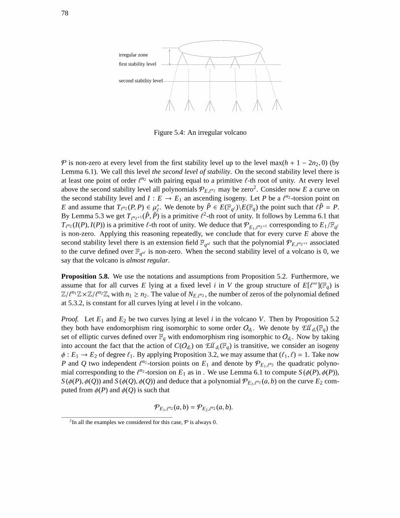
78

irregular zone

first stability level

second stability level

Figure 5.4: An irregular volcano

P is non-zero at every level from the first stability level up to the level max(h + 1 − 2n2,0) (byLemma 6.1). We call this levelthe second level of stability. On the second stability level there isat least one point of orderℓn2 with pairing equal to a primitiveℓ-th root of unity. At every levelabove the second stability level all polynomialsPE,ℓn2 may be zero2. Consider nowE a curve onthe second stability level andI : E → E1 an ascending isogeny. LetP be aℓn2-torsion point onE and assume thatTℓn2 (P,P) ∈ µ∗

ℓ. We denote byP ∈ E(Fqℓ)\E(Fq) the point such thatℓP = P.

By Lemma 5.3 we getTℓn2+1(P, P) is a primitiveℓ2-th root of unity. It follows by Lemma 6.1 thatTℓn2 (I (P), I (P)) is a primitiveℓ-th root of unity. We deduce thatPE1,ℓ

n2+1 corresponding toE1/Fqℓ

is non-zero. Applying this reasoning repeatedly, we conclude that for every curveE above thesecond stability level there is an extension fieldFqsℓ such that the polynomialPE,ℓn2+s associatedto the curve defined overFqsℓ is non-zero. When the second stability level of a volcano is 0, wesay that the volcano isalmost regular.

Proposition 5.8. We use the notations and assumptions from Proposition 5.2. Furthermore, weassume that for all curvesE lying at a fixed leveli in V the group structure ofE[ℓ∞](Fq) isZ/ℓn1Z×Z/ℓn2Z, with n1 ≥ n2. The value ofNE,ℓn2 , the number of zeros of the polynomial definedat 5.3.2, is constant for all curves lying at leveli in the volcano.

Proof. Let E1 andE2 be two curves lying at leveli in the volcanoV. Then by Proposition 5.2they both have endomorphism ring isomorphic to some orderOdi . We denote byEll di (Fq) theset of elliptic curves defined overFq with endomorphism ring isomorphic toOdi . Now by takinginto account the fact that the action ofC(Odi ) on Ell di (Fq) is transitive, we consider an isogenyφ : E1→ E2 of degreeℓ1. By applying Proposition 3.2, we may assume that (ℓ1, ℓ) = 1. Take nowP and Q two independentℓn2-torsion points onE1 and denote byPE1,ℓ

n2 the quadratic polyno-mial corresponding to theℓn2-torsion onE1 as in . We use Lemma 6.1 to computeS(φ(P), φ(P)),S(φ(P), φ(Q)) andS(φ(Q), φ(Q)) and deduce that a polynomialPE2,ℓ

n2 (a,b) on the curveE2 com-puted fromφ(P) andφ(Q) is such that

PE1,ℓn2 (a,b) = PE2,ℓ

n2 (a,b).

2In all the examples we considered for this case,P is always 0.

79

This means thatNE1,ℓn2 and NE2,ℓ

n2 coincide, which concludes the proof. Moreover, we haveshowed that the value ofk for two curves lying on the same level of a volcano is the same.

Proposition 5.9. Let E be an elliptic curve defined a finite fieldFq and letE[ℓ∞](Fq) be isomorphicto Z/ℓn1Z × Z/ℓn2Z with ℓ ≥ 3 andn1 ≥ n2 ≥ 1. SupposeNE,ℓn2 ∈ 1,2 and letP be aℓn2-torsionpoint with degenerate self-pairing. Then theℓ-isogeny whose kernel is generated byℓn2−1P iseither ascending or horizontal. Moreover, for anyℓn2-torsion pointQ whose self-pairing is non-degenerate, the isogeny with kernel spanned by< ℓn2−1Q > is descending.

Proof. Case 1.SupposeTℓn2 (P,P) ∈ µℓk, k ≥ 1 and thatTℓn2 (Q,Q) ∈ µℓk+1\µℓk. Denote byI1 : E→ E1 the isogeny whose kernel is generated byℓn2−1P andI2 : E→ E2 the isogeny whosekernel is generated byℓn2−1Q. By repeatedly applying lemmas 5.3 and 6.1, we get the followingrelations for points generating theℓn2−1-torsion onE1 andE2:

Tℓn2−1(I1(P), I1(P)) ∈ µℓk−1, Tℓn2−1(ℓI1(Q), ℓI1(Q)) ∈ µℓk−2\µℓk−3

Tℓn2−1(ℓI2(P), ℓI2(P)) ∈ µℓk−3, Tℓn2−1(I2(Q), I2(Q)) ∈ µℓk\µℓk−1.

with the convention thatµℓe = ∅ whenevere ≤ 0. From the relations above, we deduce that ontheℓ-volcano havingE,E1 andE2 as vertices,E1 andE2 do not lie at the same level. Given thefact that there are at leastℓ − 1 descending rationalℓ-isogenies parting fromE and thatQ is anyof theℓ − 1 (or more)ℓn2-torsion points with non-degenerate self-pairing, we conclude thatI1 ishorizontal or ascending and thatI2 is descending.Case 2.Suppose now thatk = 0. Note that the casen2 = 1 was already treated in Proposition 5.6.Otherwise, consider the curveE defined overFqℓ . By Lemma 5.3 we havek = 1 for points onE/Fqℓ , so we may apply Case 1.

Remark5.3. The statement at point (b) of Lemma 5.3 is not true forℓ = 2. The statements inPropositions 5.6 and 5.8 are also true forℓ = 2. Note also that all statements in the proof ofCase1 of Proposition 5.9 are true forℓ = 2 also. The only case that is not clear is the one whenk = 0andn2 ≥ 1. We did not find a proof for the statement in Proposition 5.7 forℓ = 2, but in ourcomputations with MAGMA [68] we did not find any counterexamples either.

A special case.If E is a curve lying under the first stability level and such that

E[ℓ∞](Fq) ≃ Z/ℓn1Z × Z/ℓn2Z,

with n1 > n2, then it suffices to find a pointP1 of orderℓn1 and the pointℓn1−1P1 generates thekernel of an horizontal or ascending isogeny (P1 has degenerate self-pairing).

Crater detection.Note that whenℓ is split inOE, there are two horizontal isogenies fromE andthis is equivalent, by Propositions 5.8 and 5.9, toNE,ℓn2 = 2. Similarly, whenℓ is inert inOE, thereare neither ascending nor horizontal isogenies andNE,ℓn2 = 0. In these two cases, we easily detectthat the curveE is on the crater. These results are summarized in Table 5.1.

Remark5.4. The results presented in this section hold for all curves, regardless of the value of thediscriminant of the endomorphism ring. In particular, they hold for discriminants−3,−4.

80

Table 5.1: Number of roots ofPE,ℓn2 on the volcano

NE,ℓn2 Types of isogenies Level

22→

0ℓ − 1 ↓

11→ or 1↑

i, 0 ≤ i ≤ h− 1ℓ ↓

0 ℓ + 1 ↓ 0ℓ + 1 undecided > second stability level

5.3.3 Numeric examples

In this section we give some examples in order to illustrate the results obtained in the previoussection. We do not sketch volcanoes entirely, but we give only a descending path in each case. Inour tables the notation [a,b] stands for an equation of the typey2 = x3 + ax+ b. For each curve,we give values of self-pairings for three points. Two of these points generate theℓn2-torsion, thethird one is a linear combination of the first two.

Example5.1. Let E be the elliptic curve whose Weierstrass equation is given by

y2 = x3 + 521631762x+ 248125891

defined overF1992187501. The 55-torsion is entirely defined overF1992187501. Our computationsusing pairings and Velu’s formulae gave the following volcano:

E0

E1

E2

E3

Example5.2. This example of 5-volcano that is not regular is taken from [34]. The curves aredefined overF5081. The polynomialPE0,5 is zero. Our computation showed that by consideringE0

overF50815 we get a non-zero polynomialPE0,52 and give the following volcano structure:

Example5.3. This is an example from [71] of a 2-volcano that is non-regular. Note thaton a2-volcanoes, if two self-pairings are degenerate, then any polynomialPE,2n2 is actually zero. Wetherefore make use of Kohel’s and Fouquet-Morain’s techniques to buildthe volcano until wereach the stability level 2. Then we may use pairings and Velu’s formulae to descend to the floor.

81

Level Curve Equation ℓn2 ℓn2-self-pairings isogeny type

0 E0 [521631762,248125891] 55P = (1913305198,8982844016),T55(P,P) ∈ µ55\µ54 ↓

Q = (476410925,1792947402),T55(Q,Q) ∈ µ54 →R= (1833840623,747120419),T55(R,R) ∈ µ54 →

0 E3 [1154518985,1671760359] 55P = (1193992046,1078004656),T55(P,P) ∈ µ55\µ54 ↓

Q = (1888999464,1539567655),T55(Q,Q) ∈ µ54 →R= (1049479475,786278403),T55(R,R) ∈ µ54 →

1 E1 [13045695,1561617081] 54P = (1498339142,899662653),T54(P,P) ∈ µ52 ↑

Q = (537818240,209505883),T54(Q,Q) ∈ µ54\µ53 ↓R= (303596911,620007624),T54(R,R) ∈ µ54\µ53 ↓

2 E2 [951374589,1320401943] 53P = (881997308,908148660),T53(P,P) = 1 ↑

Q = (1032634348,321607146),T53(Q,Q) ∈ µ53\µ52 →R= (1027305622,1924912950),T53(R,R) ∈ µ53\µ52 →

E0

E1

E2

Level Curve Equation ℓn2 ℓn2-self-pairings isogeny type

0 E0 [1355,2505] 5P = (4036,3650),T5(P,P) = 1 undeterminedQ = (3811,2838),T5(Q,Q) = 1 undeterminedR= (1470,2065),T5(R,R) = 1 undetermined

1 E1 [3688,3542] 5P = (4675,4827),T5(P,P) ∈ µ5\1 ↓Q = (2005,4622),T5(Q,Q) ∈ µ5\1 ↓

R= (4681,3860),T5(R,R) = 1 ↑

2 E2 [3332,4679] − − −

5.3.4 Walking on the volcano: new algorithms

In our algorithms, we first need to choose an extension field ofFq to guarantee that the kernels ofall required isogenies are spanned byℓ-torsion points defined on this extension field. As explainedin Corollary 5.1, the degree of this extension field is the order ofq moduloℓ and it can be computedvery quickly after factoringq − 1. Once this is done, assuming that we are starting from a curvebelow the second level of stability, we use Algorithms 9 and 10 to find all ascending or horizontalisogenies from the initial curve. In order to walk a descending path, it suffices to choose any otherisogeny. Note that, in the subsequent steps of a descending path, in the cases where the group

82

E0 E3

E1 E2

E4

E5

Level Curve Equation ℓn2 ℓn2-self-pairings ℓ-torsion

0 E0 y2 = x3 + 206x2 + 144x 2P = (3,0), T2(P,P) = 1 undetermined

Q = (48,0), T2(Q,Q) = 1 undeterminedR= (0,0), T2(R,R) = 1 undetermined

0 E3 y2 = x3 + 206x2 + 195x+ 78 2P = (51,0), T2(P,P) = 1 undeterminedQ = (24,0), T2(Q,Q) = 1 undeterminedR= (233,0), T2(R,R) = 1 undetermined

1 E1 y2 = x3 + 206x2 + 48x+ 224 2P = (45,0), T2(P,P) = 1 undetermined


1 E2 y2 = x3 + 206x2 + 138x+ 150 2P = (10,0), T2(P,P) = 1 undetermined


2 E4 y2 = x3 + 206x2 + 221x+ 33 2P = (121,0), T2(P,P) ∈ µ2\1 ↓

Q = (31,0), T2(Q,Q) = 1 ↑R= (156,0), T2(R,R) ∈ µ2\1 ↓

3 E5 y2 = x3 + 206x2 + 37x+ 66 − − −

structure satisfiesn1 > n2, it is not necessary to run Algorithm 10 as a whole. Indeed, since weknow that we are not on the crater, there is a single ascending isogeny and it is spanned byℓn1−1P1.In order to walk an ascending or horizontal path, it suffices to choose one of the isogenies foundby Algorithm 10, taking care not to backtrack.

5.4 Complexities and efficiency comparison

Before analyzing the complete algorithms, we first compare the costs of takinga single step ona volcano by using the two methods existing in the literature: modular polynomials and classicalVelu’s formulae. Suppose that we wish to take a step from a curveE. With the modular poly-nomial approach, we have to evaluate the polynomialf (X) = Φℓ(X, j(E)) and find its roots inFq. Assuming that the modular polynomial (modulo the characteristic ofFq) is given as inputand using asymptotically fast algorithms to factorf (X), the cost of a step in terms of arithmetic

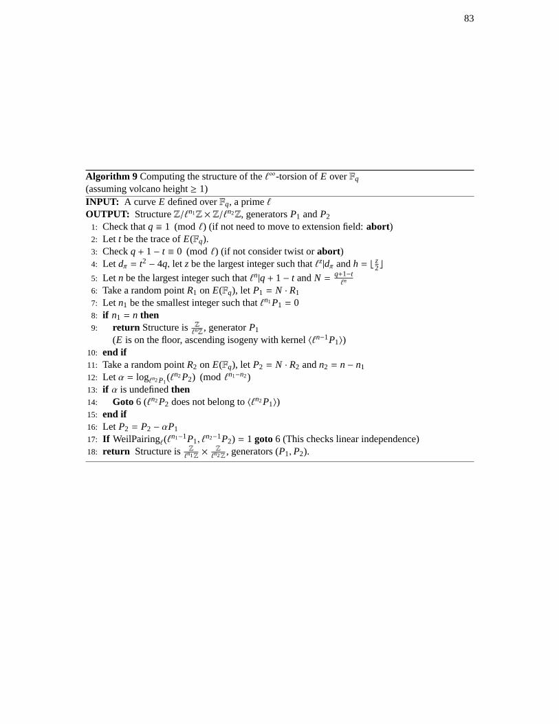
83

Algorithm 9 Computing the structure of theℓ∞-torsion ofE overFq

(assuming volcano height≥ 1)INPUT: A curveE defined overFq, a primeℓOUTPUT: StructureZ/ℓn1Z × Z/ℓn2Z, generatorsP1 andP2

1: Check thatq ≡ 1 (modℓ) (if not need to move to extension field:abort)2: Let t be the trace ofE(Fq).3: Checkq+ 1− t ≡ 0 (modℓ) (if not consider twist orabort)4: Let dπ = t2 − 4q, let z be the largest integer such thatℓz|dπ andh = ⌊ z

2⌋5: Let n be the largest integer such thatℓn|q+ 1− t andN = q+1−t

ℓn

6: Take a random pointR1 on E(Fq), let P1 = N · R1

7: Let n1 be the smallest integer such thatℓn1P1 = 08: if n1 = n then9: return Structure is Z

ℓnZ, generatorP1

(E is on the floor, ascending isogeny with kernel〈ℓn−1P1〉)10: end if11: Take a random pointR2 on E(Fq), let P2 = N · R2 andn2 = n− n1

12: Let α = logℓn2P1(ℓn2P2) (mod ℓn1−n2)

13: if α is undefinedthen14: Goto 6 (ℓn2P2 does not belong to〈ℓn2P1〉)15: end if16: Let P2 = P2 − αP1

17: If WeilPairingℓ(ℓn1−1P1, ℓ

n2−1P2) = 1 goto6 (This checks linear independence)18: return Structure is Z

ℓn1Z× Z

ℓn2Z, generators (P1,P2).

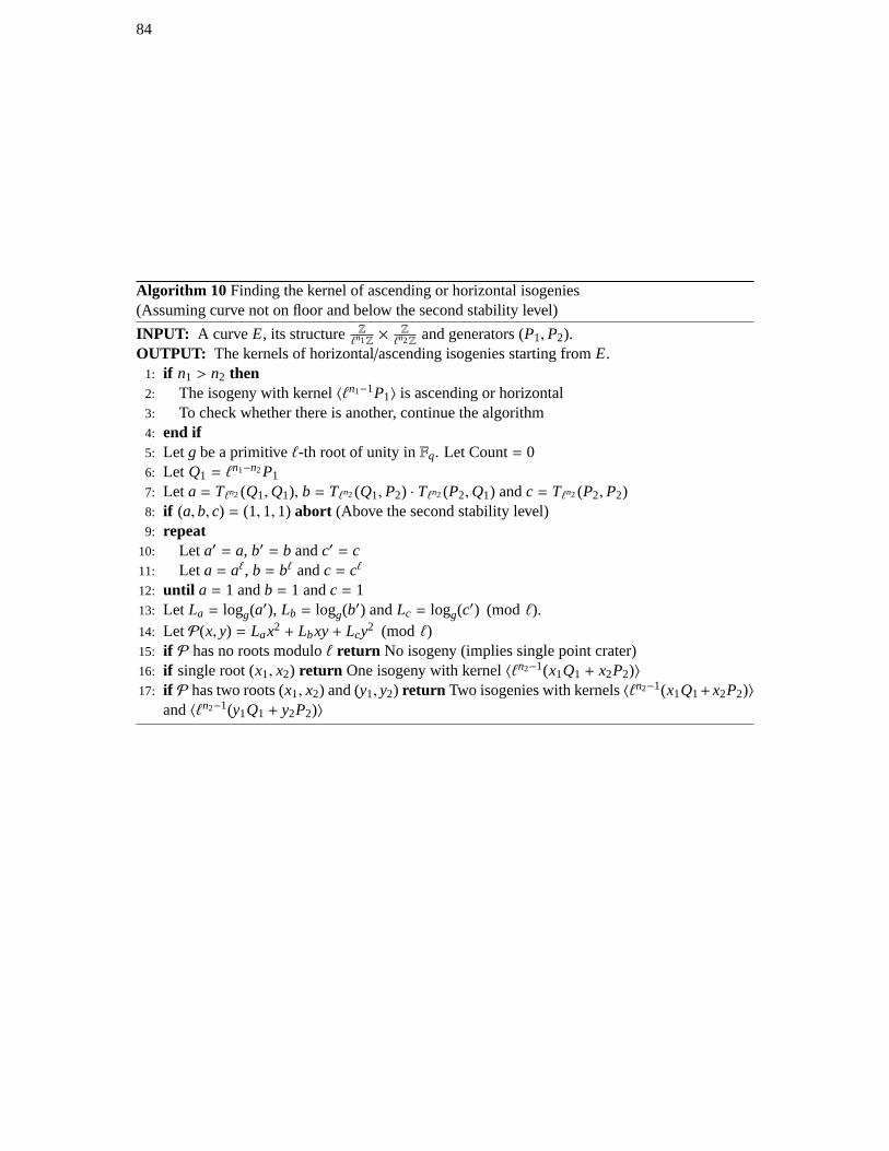
84

Algorithm 10 Finding the kernel of ascending or horizontal isogenies(Assuming curve not on floor and below the second stability level)

INPUT: A curveE, its structure Zℓn1Z× Z

ℓn2Zand generators (P1,P2).

OUTPUT: The kernels of horizontal/ascending isogenies starting fromE.1: if n1 > n2 then2: The isogeny with kernel〈ℓn1−1P1〉 is ascending or horizontal3: To check whether there is another, continue the algorithm4: end if5: Let g be a primitiveℓ-th root of unity inFq. Let Count= 06: Let Q1 = ℓ

n1−n2P1

7: Let a = Tℓn2 (Q1,Q1), b = Tℓn2 (Q1,P2) · Tℓn2 (P2,Q1) andc = Tℓn2 (P2,P2)8: if (a,b, c) = (1,1,1) abort (Above the second stability level)9: repeat

10: Let a′ = a, b′ = b andc′ = c11: Let a = aℓ, b = bℓ andc = cℓ

12: until a = 1 andb = 1 andc = 113: Let La = logg(a′), Lb = logg(b′) andLc = logg(c′) (mod ℓ).14: LetP(x, y) = Lax2 + Lbxy+ Lcy2 (mod ℓ)15: if P has no roots moduloℓ return No isogeny (implies single point crater)16: if single root (x1, x2) return One isogeny with kernel〈ℓn2−1(x1Q1 + x2P2)〉17: if P has two roots (x1, x2) and (y1, y2) return Two isogenies with kernels〈ℓn2−1(x1Q1+x2P2)〉

and〈ℓn2−1(y1Q1 + y2P2)〉

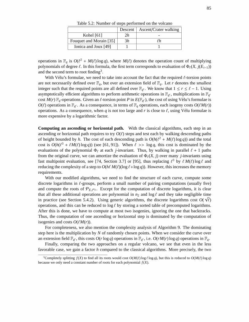
85

Table 5.2: Number of steps performed on the volcano

Descent Ascent/Crater walkingKohel [61] 2h -

Fouquet and Morain [35] 3h ℓhIonica and Joux [49] 1 1

operations inFq is O(ℓ2 + M(ℓ) logq), whereM(ℓ) denotes the operation count of multiplyingpolynomials of degreeℓ. In this formula, the first term corresponds to evaluation ofΦℓ(X, j(Ei−1))and the second term to root finding3.

With Velu’s formulae, we need to take into account the fact that the requiredℓ-torsion pointsare not necessarily defined overFq, but over an extension field ofFq. Let r denotes the smallestinteger such that the required points are all defined overFqr . We know that 1≤ r ≤ ℓ − 1. Usingasymptotically efficient algorithms to perform arithmetic operations inFqr , multiplications inFqr

costM(r) Fq-operations. Given anℓ-torsion pointP in E(Fqr ), the cost of using Velu’s formulae isO(ℓ) operations inFqr . As a consequence, in terms ofFq operations, each isogeny costsO(ℓM(r))operations. As a consequence, whenq is not too large andr is close toℓ, using Velu formulae ismore expensive by a logarithmic factor.

Computing an ascending or horizontal path. With the classical algorithms, each step in anascending or horizontal path requires to tryO(ℓ) steps and test each by walking descending pathsof height bounded byh. The cost of each descending path isO(h(ℓ2 + M(ℓ) logq)) and the totalcost isO(h(ℓ3 + ℓM(ℓ) logq)) (see [61, 91]). Whenℓ >> logq, this cost is dominated by theevaluations of the polynomialΦℓ at eachj-invariant. Thus, by walking in parallelℓ + 1 pathsfrom the original curve, we can amortize the evaluation ofΦℓ(X, j) over manyj-invariants usingfast multipoint evaluation, see [74, Section 3.7] or [95], thus replacingℓ3 by ℓ M(ℓ) logℓ andreducing the complexity of a step toO(hℓ M(ℓ)(logℓ+logq)). However, this increases the memoryrequirements.

With our modified algorithms, we need to find the structure of each curve, compute somediscrete logarithms inℓ-groups, perform a small number of pairing computations (usually five)and compute the roots ofPE,ℓn2 . Except for the computation of discrete logarithms, it is clearthat all these additional operations are polynomial inn2 and logℓ and they take negligible timein practice (see Section 5.4.2). Using generic algorithms, the discrete logarithms costO(

√ℓ)

operations, and this can be reduced to logℓ by storing a sorted table of precomputed logarithms.After this is done, we have to compute at most two isogenies, ignoring the one that backtracks.Thus, the computation of one ascending or horizontal step is dominated by thecomputation ofisogenies and costsO(ℓM(r)).

For completeness, we also mention the complexity analysis of Algorithm 9. The dominatingstep here is the multiplication byN of randomly chosen points. When we consider the curve overan extension fieldFqr , this costsO(r logq) operations inFqr , i.e. O(rM(r) logq) operations inFq.

Finally, comparing the two approaches on a regular volcano, we see that even in the lessfavorable case, we gain a factorh compared to the classical algorithms. More precisely, the two

3Completely splittingf (X) to find all its roots would costO(M(ℓ) logℓ logq), but this is reduced toO(M(ℓ) logq)because we only need a constant number of roots for each polynomialf (X).

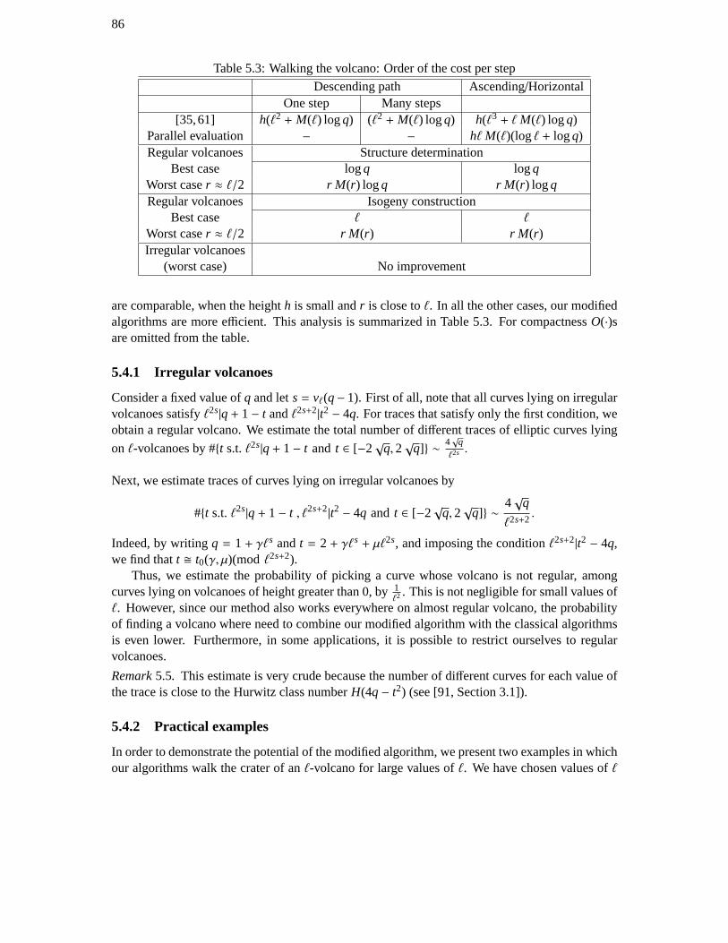
86

Table 5.3: Walking the volcano: Order of the cost per step

Descending path Ascending/HorizontalOne step Many steps

[35,61] h(ℓ2 + M(ℓ) logq) (ℓ2 + M(ℓ) logq) h(ℓ3 + ℓ M(ℓ) logq)Parallel evaluation – – hℓ M(ℓ)(logℓ + logq)Regular volcanoes Structure determination

Best case logq logqWorst caser ≈ ℓ/2 r M(r) logq r M(r) logqRegular volcanoes Isogeny construction

Best case ℓ ℓ

Worst caser ≈ ℓ/2 r M(r) r M(r)Irregular volcanoes

(worst case) No improvement

are comparable, when the heighth is small andr is close toℓ. In all the other cases, our modifiedalgorithms are more efficient. This analysis is summarized in Table 5.3. For compactnessO(·)sare omitted from the table.

5.4.1 Irregular volcanoes

Consider a fixed value ofq and lets= vℓ(q− 1). First of all, note that all curves lying on irregularvolcanoes satisfyℓ2s|q+ 1− t andℓ2s+2|t2 − 4q. For traces that satisfy only the first condition, weobtain a regular volcano. We estimate the total number of different traces of elliptic curves lying

on ℓ-volcanoes by #t s.t.ℓ2s|q+ 1− t and t ∈ [−2√

q,2√

q] ∼ 4√

qℓ2s .

Next, we estimate traces of curves lying on irregular volcanoes by

#t s.t.ℓ2s|q+ 1− t , ℓ2s+2|t2 − 4q and t ∈ [−2√

q,2√

q] ∼4√

q

ℓ2s+2.

Indeed, by writingq = 1+ γℓs andt = 2+ γℓs + µℓ2s, and imposing the conditionℓ2s+2|t2 − 4q,we find thatt t0(γ, µ)(mod ℓ2s+2).

Thus, we estimate the probability of picking a curve whose volcano is not regular, amongcurves lying on volcanoes of height greater than 0, by1

ℓ2 . This is not negligible for small values ofℓ. However, since our method also works everywhere on almost regular volcano, the probabilityof finding a volcano where need to combine our modified algorithm with the classical algorithmsis even lower. Furthermore, in some applications, it is possible to restrict ourselves to regularvolcanoes.

Remark5.5. This estimate is very crude because the number of different curves for each value ofthe trace is close to the Hurwitz class numberH(4q− t2) (see [91, Section 3.1]).

5.4.2 Practical examples

In order to demonstrate the potential of the modified algorithm, we present two examples in whichour algorithms walk the crater of anℓ-volcano for large values ofℓ. We have chosen values ofℓ

87

for which the modular polynomial approach is expensive, in both time and memory (see [88] forprecomputations of modular polynomials).

A favorable case. We consider the favorable case of a volcano of height 2, where all the neces-saryℓ-torsion points are defined over the base fieldFp, wherep = 619074283342666852501391is prime. We chooseℓ = 100003.Let E be the elliptic curve whose Weierstrass equation is

y2 = x3 + 198950713578094615678321x+ 32044133215969807107747.

The groupE[ℓ∞] overFp has structureZℓ4Z. It is spanned by the point

P = (110646719734315214798587,521505339992224627932173).

Taking theℓ-isogenyI1 with kernel〈ℓ3P〉, we obtain the curve

E1 : y2 = x3 + 476298723694969288644436x+ 260540808216901292162091,

with structure of theℓ∞-torsion Zℓ3 × Zℓ and generators

P1 = (22630045752997075604069,207694187789705800930332) and

Q1 = (304782745358080727058129,193904829837168032791973).

Theℓ-isogenyI2 with kernel〈ℓ2P1〉 leads to the curve

E2 : y2 = x3 + 21207599576300038652790x+ 471086215466928725193841,

on the volcano’s crater and with structureZℓ2Z× Z

ℓ2Zand generators

P2 = (545333002760803067576755,367548280448276783133614) and

Q2 = (401515368371004856400951,225420044066280025495795).

Using pairings on these points, we construct the polynomial:

P(x, y) = 97540x2 + 68114x y+ 38120y2,

having homogeneous roots (x, y) = (26568,1) and (72407,1). As a consequence, we have twohorizontal isogenies with kernels〈ℓ(26568P2 + Q2)〉 and〈ℓ(72407P2 + Q2)〉. We can continueand make a complete walk around the crater which contains 22 different curves. Using a crudeimplementation under Magma 2.15-15, a typical execution takes about 154 seconds4 on a singlecore of an Intel Core 2 Duo at 2.66 GHz. Most of the time is taken by the computation of Velu’sformulas (138.3 seconds) and the computation of discrete logarithms (15.2 seconds) which are nottabulated in the implementation. The computation of pairings only takes 40 milliseconds.

4This timing varies between executions. The reason that we first try one root ofP, if it backtracks on the crater, weneed to try the other one. On average, 1.5 root is tried for each step, but this varies depending on the random choices.

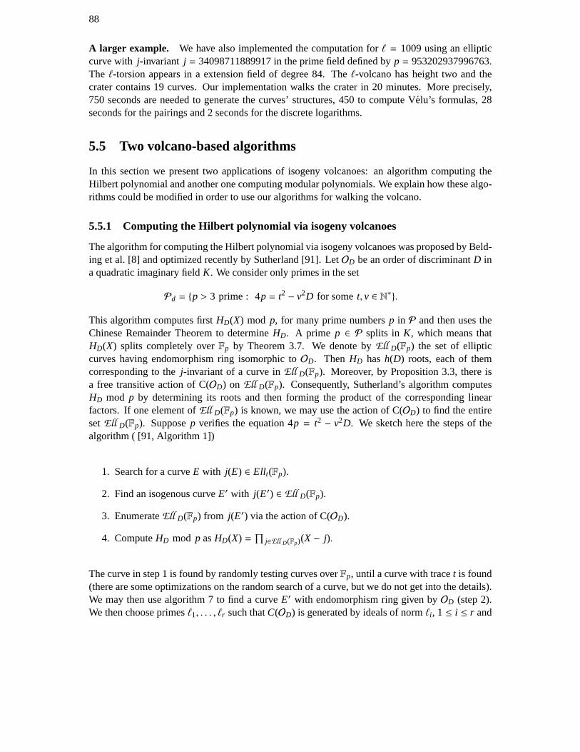
88

A larger example. We have also implemented the computation forℓ = 1009 using an ellipticcurve with j-invariant j = 34098711889917 in the prime field defined byp = 953202937996763.The ℓ-torsion appears in a extension field of degree 84. Theℓ-volcano has height two and thecrater contains 19 curves. Our implementation walks the crater in 20 minutes. More precisely,750 seconds are needed to generate the curves’ structures, 450 to compute Velu’s formulas, 28seconds for the pairings and 2 seconds for the discrete logarithms.

5.5 Two volcano-based algorithms

In this section we present two applications of isogeny volcanoes: an algorithm computing theHilbert polynomial and another one computing modular polynomials. We explain how these algo-rithms could be modified in order to use our algorithms for walking the volcano.

5.5.1 Computing the Hilbert polynomial via isogeny volcanoes

The algorithm for computing the Hilbert polynomial via isogeny volcanoes wasproposed by Beld-ing et al. [8] and optimized recently by Sutherland [91]. LetOD be an order of discriminantD ina quadratic imaginary fieldK. We consider only primes in the set

Pd = p > 3 prime : 4p = t2 − v2D for somet, v ∈ N∗.

This algorithm computes firstHD(X) mod p, for many prime numbersp in P and then uses theChinese Remainder Theorem to determineHD. A prime p ∈ P splits in K, which means thatHD(X) splits completely overFp by Theorem 3.7. We denote byEll D(Fp) the set of ellipticcurves having endomorphism ring isomorphic toOD. Then HD hash(D) roots, each of themcorresponding to thej-invariant of a curve inEll D(Fp). Moreover, by Proposition 3.3, there isa free transitive action of C(OD) on Ell D(Fp). Consequently, Sutherland’s algorithm computesHD mod p by determining its roots and then forming the product of the corresponding linearfactors. If one element ofEll D(Fp) is known, we may use the action of C(OD) to find the entiresetEll D(Fp). Supposep verifies the equation 4p = t2 − v2D. We sketch here the steps of thealgorithm ( [91, Algorithm 1])

1. Search for a curveE with j(E) ∈ Ellt(Fp).

2. Find an isogenous curveE′ with j(E′) ∈ Ell D(Fp).

3. EnumerateEll D(Fp) from j(E′) via the action of C(OD).

4. ComputeHD mod p asHD(X) =∏

j∈Ell D(Fp)(X − j).

The curve in step 1 is found by randomly testing curves overFp, until a curve with tracet is found(there are some optimizations on the random search of a curve, but we do not get into the details).We may then use algorithm 7 to find a curveE′ with endomorphism ring given byOD (step 2).We then choose primesℓ1, . . . , ℓr such thatC(OD) is generated by ideals of normℓi , 1 ≤ i ≤ r and

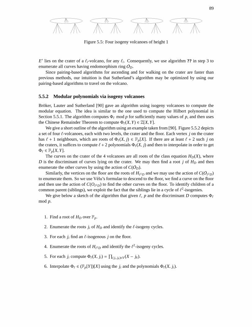
89

Figure 5.5: Four isogeny volcanoes of height 1

E′ lies on the crater of aℓi-volcano, for anyℓi . Consequently, we use algorithm?? in step 3 toenumerate all curves having endomorphism ringOD.

Since pairing-based algorithms for ascending and for walking on the crater are faster thanprevious methods, our intuition is that Sutherland’s algorithm may be optimized byusing ourpairing-based algorithms to travel on the volcano.

5.5.2 Modular polynomials via isogeny volcanoes

Broker, Lauter and Sutherland [90] gave an algorithm using isogeny volcanoes to compute themodular equation. The idea is similar to the one used to compute the Hilbert polynomial inSection 5.5.1. The algorithm computesΦℓ modp for sufficiently many values ofp, and then usesthe Chinese Remainder Theorem to computeΦℓ(X,Y) ∈ Z[X,Y].

We give a short outline of the algorithm using an example taken from [90]. Figure 5.5.2 depictsa set of fourℓ-volcanoes, each with two levels, the crater and the floor. Each vertexj on the craterhasℓ + 1 neighbours, which are roots ofΦℓ(X, j) ∈ Fp[X]. If there are at leastℓ + 2 such j onthe craters, it suffices to computeℓ + 2 polynomialsΦℓ(X, j) and then to interpolate in order to getΦℓ ∈ Fp[X,Y].

The curves on the crater of the 4 volcanoes are all roots of the class equation HD(X), whereD is the discriminant of curves lying on the crater. We may then find a rootj of HD and thenenumerate the other curves by using the action ofC(OD).

Similarly, the vertices on the floor are the roots ofHℓ2D and we may use the action ofC(Oℓ2D)to enumerate them. So we use Velu’s formulae to descend to the floor, we find a curve on the floorand then use the action ofC(Oℓ2D) to find the other curves on the floor. To identify children of acommon parent (siblings), we exploit the fact that the siblings lie in a cycle ofℓ2-isogenies.

We give below a sketch of the algorithm that givenℓ, p and the discriminantD computesΦℓmod p.

1. Find a root ofHD overFp.

2. Enumerate the rootsj i of HD and identify theℓ-isogeny cycles.

3. For eachj i find anℓ-isogenousj on the floor.

4. Enumerate the roots ofHℓ2D and identify theℓ2-isogeny cycles.

5. For eachj i computeΦℓ(X, j i) =∏

( j i , jk)∈V(X − jk).

6. InterpolateΦℓ ∈ (Fp[Y])[X] using thej i and the polynomialsΦℓ(X, j i).

90

We explain how this algorithm could be modified in order to use our pairing-based algorithms.First of all, instead of precomputingHD(X) and then factorizing this polynomial modp in step 1,we could simply search of for a curve of tracet and then use algorithm 10 to ascend to the crater.Note that we can easily recognize a curve on the crater, since the polynomialsPE,ℓn2 have tworoots if and only if we have reached the crater.

All volcanoes are regular, hence we could Velu’s formulae to enumerate all curves lying oncraters and, at the same time, compute the siblings for each of these curves.This is easy since ourpairing-based algorithms can distinguish between points spanning kernels of horizontal isogeniesand points spanning kernels of descendingℓ-isogenies. This method produces, for each curvejon the crater, the polynomialΦℓ. In order to enumerate all the curves inEll (Fp) we also need away to switch from one volcano to another. We may use, for example, the action of C(OD). Notethat no identification ofℓ-cycles orℓ2-cycles is needed in this way and that each curve inEllt(Fp)is only considered once.

Since evaluating complexities of these algorithms is an elaborated task, we do not pretend thismethod would give a faster algorithm. Further work is necessary to make the most of our approachwith pairings.

5.6 Conclusion

In this chapter, we have proposed a method which allows, in the regular part of an isogeny volcano,to determine, given a curveE and aℓ-torsion pointP, the type of theℓ-isogeny whose kernel isspanned byP. In addition, this method also permits, given a system of generators for theℓ-torsion, to find the ascending isogeny (or horizontal isogenies) fromE. Finally, our study ofvolcanoes shows that it is possible to determine the level of a curve on the volcano by simplycomputing a small number of pairings. In particular, we can easily determine if the curve lies onthe crater of the volcano. We expect that our algorithms can be used to improve the performanceof several volcano-based algorithms, such as the computation of the Hilbert’s [91] or modular [90]polynomials.

Part III

Pairings and Cryptography

91

Chapter 6

Efficient Implementation ofCryptographic Pairings

In this chapter, we study the implementation of cryptographic pairings on elliptic curves. Weshow that an efficient implementation of the pairing depends on both the choice of the curve andits parameters and on the efficient representation of points on the elliptic curve. We start by pre-senting in Section 6.2 our formulae for pairing computation in Jacobian coordinates [50]. Weexplain that for curves with even embedding degrees, pairing computation ismost efficient whenpoints are represented as points on the twisted curve. Further, we study endomorphisms on curveswith small embedding degree. Section 6.3 gives a brief survey ondistortion mapson ordinarycurves. Distortion maps are used in cryptography to construct non-degenerate self-pairings. First,we show that due to results obtained in our study of isogeny volcanoes in Chapter 5, it is possibleto construct curves with non-degenerate self-pairings without using distortions (Section 6.4). Sec-ondly, we implicitly obtain subgroups on the elliptic curve which are invariant under the action ofendomorphisms. In Section 6.5 we show that in such subgroups, it is possible to use the actionof the endomorphism in order to compute the pairing efficiently. Our method applies topairingfriendly curvesconstructed by the Cocks-Pinch method presented in Chapter 4.

6.1 Pairings in cryptography

A secure pairing-based cryptosystem needs to be implemented in elliptic curvesubgroupsG1 andG2 with a pairing

e : G1 × G2→ H,

such that the discrete logarithm problem is computationally difficult in G1, G2 and inH ∈ F∗qk.

The best known algorithm for computing discrete logarithms on elliptic curves isthe Pollard-rhomethod [76, 79], which has complexityO(

√r), wherer is the order of the groupsG1 andG2.

Meanwhile, the best known algorithm for solving the discrete logarithm problem in the multi-plicative group of a finite field is the index calculus algorithm, which has sub-exponential runningtime [52,53]. Consequently, in order to achieve the same level of security inboth the elliptic curvesubgroups and in the finite field subgroup, we need to choose aqk which is significantly larger

93

94

thanr. It is therefore interesting to consider the ratio of these sizes:

klog qlog r

.

As the efficiency of the implementation will depend critically on the so-calledρ-value

ρ =logqlog r

,

it is preferable to keep this value as small as possible and increase the valueof the embeddingdegreek, whenever we want a higher level of security the finite field. The followingdefinition isgiven by Teske et al. [36].

Definition 6.1. Let E be a curve defined over a finite fieldFq. We say thatE is pairing friendly ifthe following two conditions hold:

(a) there is a primer dividing E(Fq) such thatr ≥ √q;

(b) the embedding degree with respect tor is less than (logr)/8.

Teske et al. justify the bound on the size ofr in this definition by giving a result due to Lucaand Shparlinski [67], who showed that curves having small embedding degree are abundant ifr <

√q and rare ifr >

√q. The bound onk is based on the requirements for different desired

security levels (see [36] for details).In Chapter 4, we have presented the Cocks-Pinch method to construct curves with small em-

bedding degree andρ-value 2. Research in pairing-based cryptography during the past few years,has focussed on finding pairing-friendly curves whoseρ-value is closer to 1. Up to now, a smallnumber of examples are known. Miyaji, Nakabayashi and Takano [73] found examples of curveswith embedding degrees 3,4,6 andρ ≈ 1, but such curves are very rare. In an exhaustive searchfor such curves, the value of the discriminant of the endomorphism ring ofthe curve grows veryquickly (see [57] and [67]). Barreto and Naehrig [7] gave an exampleof curves withρ-value 1and embedding degree 12. Other examples of families of curves with smallρ-value were foundby Kachisa et al. [56] for embedding degrees 16 and 18. The reader should refer to [36] fora survey of all families of pairing friendly curves withρ-value close to 1. However, note thatVercauteren [36] showed recently that for some discriminants there are no ordinary curves withρ-value smaller than 2.

Proposition 6.1. Let E be an elliptic curve overFq with a subgroup of prime orderr > 3 andembedding degreek > 1 with respect tor. If E has a twistE′/Fq of degreek andr ≥ 4

√q, thenE

is supersingular.

Proof. See [36, Prop. 7.1].

In particular, this means that there are no ordinary curves with embedding degree 2 andρ-value smaller than 2. Moreover, ordinary curves with discriminant−4 and embedding degree 4and those with discriminant−3 and embedding degree 6 haveρ-value at least 2.

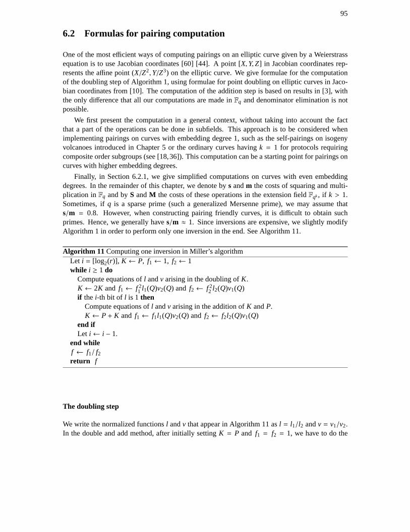
95

6.2 Formulas for pairing computation

One of the most efficient ways of computing pairings on an elliptic curve given by a Weierstrassequation is to use Jacobian coordinates [60] [44]. A point [X,Y,Z] in Jacobian coordinates rep-resents the affine point (X/Z2,Y/Z3) on the elliptic curve. We give formulae for the computationof the doubling step of Algorithm 1, using formulae for point doubling on ellipticcurves in Jaco-bian coordinates from [10]. The computation of the addition step is based onresults in [3], withthe only difference that all our computations are made inFq and denominator elimination is notpossible.

We first present the computation in a general context, without taking into account the factthat a part of the operations can be done in subfields. This approach is tobe considered whenimplementing pairings on curves with embedding degree 1, such as the self-pairings on isogenyvolcanoes introduced in Chapter 5 or the ordinary curves havingk = 1 for protocols requiringcomposite order subgroups (see [18,36]). This computation can be a starting point for pairings oncurves with higher embedding degrees.

Finally, in Section 6.2.1, we give simplified computations on curves with even embeddingdegrees. In the remainder of this chapter, we denote bys andm the costs of squaring and multi-plication inFq and byS andM the costs of these operations in the extension fieldFqk, if k > 1.Sometimes, ifq is a sparse prime (such a generalized Mersenne prime), we may assume thats/m = 0.8. However, when constructing pairing friendly curves, it is difficult to obtain suchprimes. Hence, we generally haves/m ≈ 1. Since inversions are expensive, we slightly modifyAlgorithm 1 in order to perform only one inversion in the end. See Algorithm 11.

Algorithm 11 Computing one inversion in Miller’s algorithmLet i = [log2(r)], K ← P, f1← 1, f2← 1while i ≥ 1 do

Compute equations ofl andv arising in the doubling ofK.K ← 2K and f1← f 2

1 l1(Q)v2(Q) and f2← f 22 l2(Q)v1(Q)

if the i-th bit of l is 1 thenCompute equations ofl andv arising in the addition ofK andP.K ← P+ K and f1← f1l1(Q)v2(Q) and f2← f2l2(Q)v1(Q)

end ifLet i ← i − 1.

end whilef ← f1/ f2return f

The doubling step

We write the normalized functionsl andv that appear in Algorithm 11 asl = l1/l2 andv = v1/v2.In the double and add method, after initially settingK = P and f1 = f2 = 1, we have to do the

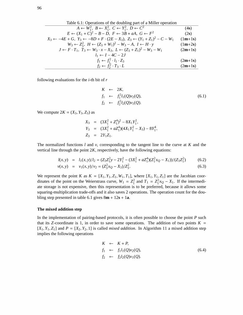
96

Table 6.1: Operations of the doubling part of a Miller operationA←W2

1 , B← X21, C← Y2

1 , D← C2 (4s)E← (X1 +C)2 − B− D, F ← 3B+ aA, G← F2 (2s)

X3← −4E +G, Y3← −8D + F · (2E − X3), Z3← (Y1 + Z1)2 −C −W1 (1m+1s)W3← Z2

3, H ← (Z3 +W1)2 −W3 − A, I ← H · y (1m+2s)J← F · T1, T3←W3 · x− X3, L← (Z3 + Z1)2 −W3 −W1 (2m+1s)

l1← I − 4C − 2Jf1← f 2

1 · l1 · Z3 (2m+1s)f2← f 2

2 · T3 · L (2m+1s)

following evaluations for thei-th bit of r

K ← 2K,

f1 ← f 21 l1(Q)v2(Q), (6.1)

f2 ← f 22 l2(Q)v1(Q).

We compute 2K = (X3,Y3,Z3) as

X3 = (3X21 + Z4

1)2 − 8X1Y21 ,

Y3 = (3X21 + aZ4

1)(4X1Y21 − X3) − 8Y4

1 ,

Z3 = 2Y1Z1.

The normalized functionsl and v, corresponding to the tangent line to the curve atK and thevertical line through the point 2K, respectively, have the following equations:

l(x, y) = l1(x, y)/l2 = (Z3Z21y− 2Y2

1 − (3X21 + aZ4

1)(Z21xQ − X1))/(Z3Z2

1) (6.2)

v(x, y) = v1(x, y)/v2 = (Z23xQ − X3)/Z2

3. (6.3)

We represent the pointK as K = [X1,Y1,Z1,W1,T1], where [X1,Y1,Z1] are the Jacobian coor-dinates of the point on the Weierstrass curve,W1 = Z2

1 andT1 = Z21xQ − X1. If the intermedi-

ate storage is not expensive, then this representation is to be preferred, because it allows somesquaring-multiplication trade-offs and it also saves 2 operations. The operation count for the dou-bling step presented in table 6.1 gives 8m + 12s+ 1a.

The mixed addition step

In the implementation of pairing-based protocols, it is often possible to choosethe pointP suchthat its Z-coordinate is 1, in order to save some operations. The addition of two pointsK =[X1,Y1,Z1] and P = [X2,Y2,1] is calledmixed addition. In Algorithm 11 a mixed addition stepimplies the following operations

K ← K + P,

f1 ← f1l1(Q)v2(Q), (6.4)

f2 ← f2l2(Q)v1(Q).

97

Table 6.2: Operations of the addition part of a Miller operation fork > 2B← X2 ·W1, D← ((Y2 + Z1)2 − R2 −W1) ·W1, H ← B− X1, I ← H2 (2m+2s)

E← 4I , J← H · E, L1← (D − 2Y1), V ← X1 · E, K ← (Y2 + Z3)2 − R2 − T3 (2m+1s)X3← L2

1 − J − 2V; Y3← L1 · (V − X3) − 2Y1 · J (2m+1s)Z3← (Z1 + H)2 −W1 − I , W3← Z2

3, T3←W3 · xQ − X3, l1← 2Z3 · yQ − K − 2L1 · (xQ − X2) (3m+2s)f1← f1 · l1 (1m)

f2← f2 · 2Z3 (1m)

The result of the addition ofK = [X1,Y1,Z1,W1,T1] and P = [X2,Y2,1,1, xQ − X2] is K + P =[X3,Y3,Z3,W3,T3] with

X3 = (X1 + X2Z21)(X1 − X2Z2

1)2 + (Y2Z31 − Y1)2,

Y3 = (Y2Z31 − Y1)(X1(X1 − X2Z2

1)2 − X3) + Y1(X1 − X2Z21)2,

Z3 = Z1(X2Z21 − X1),

W3 = Z23,

T3 = W3xQ − X3.

The linesl andv have the following equations

l = l1/l2 = Z3y− Y2Z3 − (2Y2Z31 − 2Y1)(xQ − X2)/Z3,

v = (W3xQ − X3)/W3.

We precomputeR2 = Y22 and A = xQ − X2. Efficient mixed addition formulas were given by

Arene et al. [3]. We slightly modified their operation count in order to adapt it tothe general case.Detailed operations are presented in table 6.2 and the total cost is 11m + 6s.

6.2.1 The Case of Curves with Even Embedding Degree

Pairing computation for curves with embedding degree greater than 1 is different from the com-putation presented in the previous section, due to the fact that many computations are done insubfields ofFqk. For efficiency reasons, the pointP can be chosen such that〈P〉 is the uniquesubgroup of orderr in E(Fq). We may thus describe this subgroup as

G1 = E[r] ∩ Ker(π − [1]). (6.5)

In order to get a non-degenerate pairing, we need to defineG2 as a subgroup of orderr inE(Fqk)\E(Fq). In this section we show that by taking

G2 = E[r] ∩ Ker(π − [q]), (6.6)

we get a non-degenerate pairing, as well as an efficient implementation of Miller’s algorithm. Thefollowing result and its proof are taken from [47].

Theorem 6.1. Let E be an ordinary elliptic curve overFq admitting a twist of degreee. Assumethatr > 6 satisfiesr ||#E(Fq) andr2||#E(Fqe). Then there is a unique twistE′ of degreee such that

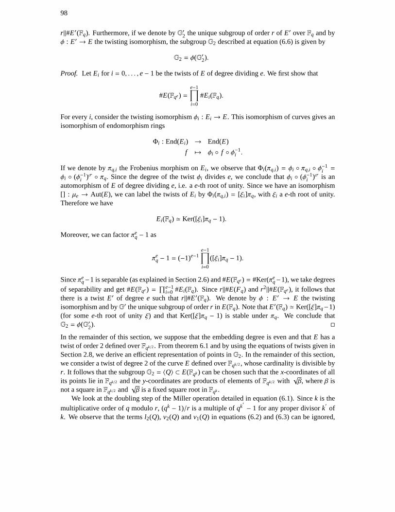
98

r ||#E′(Fq). Furthermore, if we denote byG′2 the unique subgroup of orderr of E′ overFq and byφ : E′ → E the twisting isomorphism, the subgroupG2 described at equation (6.6) is given by

G2 = φ(G′2).

Proof. Let Ei for i = 0, . . . ,e− 1 be the twists ofE of degree dividinge. We first show that

#E(Fqe) =e−1∏

i=0

#Ei(Fq).

For everyi, consider the twisting isomorphismφi : Ei → E. This isomorphism of curves gives anisomorphism of endomorphism rings

Φi : End(Ei) → End(E)

f 7→ φi f φ−1i .

If we denote byπq,i the Frobenius morphism onEi , we observe thatΦi(πq,i) = φi πq,i φ−1i =

φi (φ−1i )σ πq. Since the degree of the twistφi dividese, we conclude thatφi (φ−1

i )σ is anautomorphism ofE of degree dividinge, i.e. ae-th root of unity. Since we have an isomorphism[] : µe → Aut(E), we can label the twists ofEi by Φi(πq,i) = [ξi ]πq, with ξi a e-th root of unity.Therefore we have

Ei(Fq) ≃ Ker([ξi ]πq − 1).

Moreover, we can factorπeq − 1 as

πeq − 1 = (−1)e−1

e−1∏

i=0

([ξi ]πq − 1).

Sinceπeq−1 is separable (as explained in Section 2.6) and #E(Fqe) = #Ker(πe

q−1), we take degreesof separability and get #E(Fqe) =

∏e−1i=0 #Ei(Fq). Sincer ||#E(Fq) andr2||#E(Fqe), it follows that

there is a twistE′ of degreee such thatr ||#E′(Fq). We denote byφ : E′ → E the twistingisomorphism and byG′ the unique subgroup of orderr in E(Fq). Note thatE′(Fq) ≃ Ker([ξ]πq−1)(for somee-th root of unity ξ) and that Ker([ξ]πq − 1) is stable underπq. We conclude thatG2 = φ(G′2).

In the remainder of this section, we suppose that the embedding degree is even and thatE has atwist of order 2 defined overFqk/2. From theorem 6.1 and by using the equations of twists given inSection 2.8, we derive an efficient representation of points inG2. In the remainder of this section,we consider a twist of degree 2 of the curveE defined overFqk/2, whose cardinality is divisible byr. It follows that the subgroupG2 = 〈Q〉 ⊂ E(Fqk) can be chosen such that thex-coordinates of allits points lie inFqk/2 and they-coordinates are products of elements ofFqk/2 with

√β, whereβ is

not a square inFqk/2 and√β is a fixed square root inFqk.

We look at the doubling step of the Miller operation detailed in equation (6.1). Sincek is themultiplicative order ofq modulor, (qk − 1)/r is a multiple ofqk

′− 1 for any proper divisork

′of

k. We observe that the termsl2(Q), v2(Q) andv1(Q) in equations (6.2) and (6.3) can be ignored,

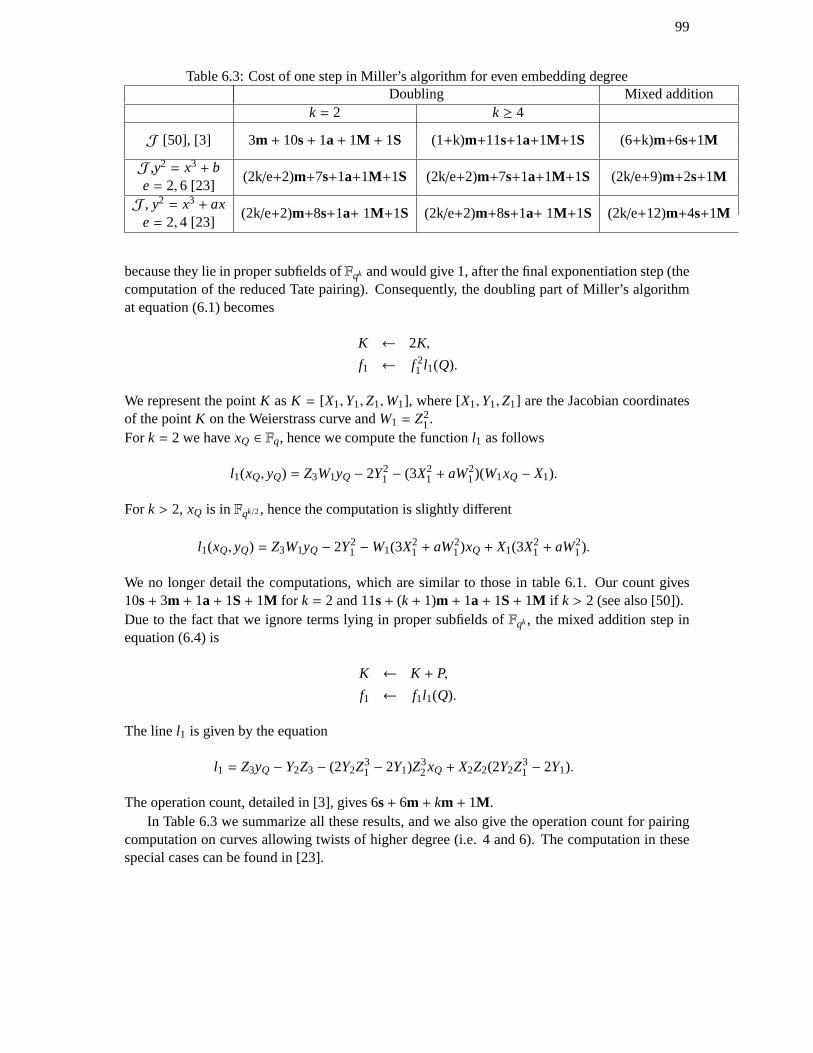
99

Table 6.3: Cost of one step in Miller’s algorithm for even embedding degreeDoubling Mixed addition

k = 2 k ≥ 4

J [50], [3] 3m + 10s+ 1a+ 1M + 1S (1+k)m+11s+1a+1M+1S (6+k)m+6s+1M

J ,y2 = x3 + b(2k/e+2)m+7s+1a+1M+1S (2k/e+2)m+7s+1a+1M+1S (2k/e+9)m+2s+1M

e= 2,6 [23]J , y2 = x3 + ax

(2k/e+2)m+8s+1a+ 1M+1S (2k/e+2)m+8s+1a+ 1M+1S (2k/e+12)m+4s+1Me= 2,4 [23]

because they lie in proper subfields ofFqk and would give 1, after the final exponentiation step (thecomputation of the reduced Tate pairing). Consequently, the doubling partof Miller’s algorithmat equation (6.1) becomes

K ← 2K,

f1 ← f 21 l1(Q).

We represent the pointK asK = [X1,Y1,Z1,W1], where [X1,Y1,Z1] are the Jacobian coordinatesof the pointK on the Weierstrass curve andW1 = Z2

1.For k = 2 we havexQ ∈ Fq, hence we compute the functionl1 as follows

l1(xQ, yQ) = Z3W1yQ − 2Y21 − (3X2

1 + aW21)(W1xQ − X1).

For k > 2, xQ is in Fqk/2, hence the computation is slightly different

l1(xQ, yQ) = Z3W1yQ − 2Y21 −W1(3X2

1 + aW21)xQ + X1(3X2

1 + aW21).

We no longer detail the computations, which are similar to those in table 6.1. Our count gives10s+ 3m + 1a+ 1S+ 1M for k = 2 and 11s+ (k+ 1)m + 1a+ 1S+ 1M if k > 2 (see also [50]).Due to the fact that we ignore terms lying in proper subfields ofFqk, the mixed addition step inequation (6.4) is

K ← K + P,

f1 ← f1l1(Q).

The linel1 is given by the equation

l1 = Z3yQ − Y2Z3 − (2Y2Z31 − 2Y1)Z3

2xQ + X2Z2(2Y2Z31 − 2Y1).

The operation count, detailed in [3], gives 6s+ 6m + km + 1M .In Table 6.3 we summarize all these results, and we also give the operation count for pairing

computation on curves allowing twists of higher degree (i.e. 4 and 6). The computation in thesespecial cases can be found in [23].

100

6.3 Self-pairings and distortion maps

We say that an endomorphismφ : E→ E is adistortion mapon E with respect to a pointP on Eif φ(P) < 〈P〉.Example6.1. We consider the curve given by the equation

y2 = x3 + ax, (6.7)

whereq ≡ 3 (mod 4). The latter condition ensures that−1 is not a square inFq. A distorsion mapfor points (x, y) defined overFq is given byφ(x, y) = (−x, iy), with i2 = −1.

The curve in Example 6.7 is supersingular. Verheul [94] showed that onsupersingular curvesall points have distortion maps.

In cryptography, special attention has been paid to distortion maps because they enable theconstruction of non-degenerate self-pairings. Indeed, in the case ofthe Tate pairing, ifTr (P,P) =1, thenTr (P, φ(P)) , 1 if φ(P) < 〈P〉. This is due to the non-degeneracy of the pairing. Firstof all, this can be used in the implementation of protocols which require pairings with G1 = G2.Secondly, this property can be used to solve the DDH hypothesis on some orderr groups. Indeed,given a 4-uple (P,aP,bP, cP), we can decide whetherab≡ c (mod r) by verifying if

Tr (aP, φ(bP)) = Tr (P, φ(cP)).

Since in this dissertation we focus on ordinary curves, we survey resultson distortion maps onthese curves. The following result is due to Charles [24].

Theorem 6.2. Let E be an ordinary elliptic curve defined over a finite fieldFq and denote byO,the endomorphism ring ofE. O is an order in a quadratic imaginary field with maximal orderOK

and discriminantdK . Supposer is a prime such thatE[r] ⊂ Fq, but no point of orderr is definedover a smaller extension field.

(a) If r | [OK : O], then there are no distortion maps.

(b) If r ∤ [OK : O]dK and

(i) r is inert inOK , then there are distortion maps for every (orderr) subgroup ofE[r];

(ii) r is split inOK , then all but two subgroups ofE[r] have distortion maps.

(c) If r ∤ [OK : O] andr |dK , so thatr is ramified inOK , then all (except one) subgroups ofE[r]have distortion maps.

Proof. It is easy to see that ifr | [OK : O] there are no distortion maps, because the reductionmodulor of every endomorphism is the multiplication by a scalar. Suppose now thatr ∤ [OK : O].We have

OK/(r) O/(r).

If r ∤ dK and r is inert inOK , thenO/(r) Fr2. We takeα ∈ O such thatα (mod r) does notlie in Fr . Then the action ofα on E[r] is irreducible overFr , since the characteristic equation isirreducible. It follows that no subgroup of orderr is stabilized byα, henceα is a distortion map

101

for all points inE[r]. If r ∤ dK andr is split inOK , thenO/(r) Fr [X]/(X − a)(X − b) (Z/rZ)2

(wherea , b). The action of anyα ∈ OK corresponds toX in Fr (X)/(X−a)(X−b) and is conjugateto a matrix of the form (

γ 00 δ

)

Distortion maps exist for all but two subgroups ofE[r]. Finally, if r is ramified,O/(r) Fr [X]/(X−a)2. Consider the mapα ∈ O that corresponds toX in the ringFr [X]/(X − a)2. Then the action ofα on E[r] is given by the matrix (

1 β

0 1

)

with β , 0. We conclude that there are distortion maps for all but one subgroup ofE[r].

Suppose now that the embedding degreek with respect tor is greater than 1. For any pointP ∈ E(Fqk), we define the trace map as

Tr(P) =k−1∑

i=0

πi(P).

This map was proposed as a distortion map in [16] and [17]. We consider twopoints P ∈ G1

andQ ∈ G2, whereG1 andG2 are the subgroups defined at equations (6.5) and (6.6). It is easyto check that forR = aP+ bQ, with ab , 0, thenTr(R) = kaP. This means that the trace is adistortion map for all points of orderr that are neither inG1, nor inG2. Verheul [94] shows thatthere are no distortion maps for points inG1 andG2.

Theorem 6.3. Let E be an ordinary curve defined overFq and letP be a point overE of primeorderr , char(Fq). Suppose the embedding degreek is greater than 1 and denote byQ the pointdefined overFqk, such thatπ(Q) = qQ. Then there are no distorsion maps forP andQ.

Proof. Suppose there is a distortionφ of 〈P〉. Then we have

φ(π(P)) = π(φ(P)) andφ(π(P)) = φ(P). (6.8)

The first equality comes from the fact that the ring End(E) is commutative, while the second oneis due to the fact thatP ∈ E(Fq). It follows thatπ(φ(P)) = φ(P), henceφ(P) is an eigenvector forthe eigenvalue 1 ofπ. This means thatφ(P) ∈ 〈P〉. The proof forQ is similar.

The conclusion is that by choosing to implement the pairing onG1 × G2, we get efficient pairingimplementation and also work in subgroups for which the DDH problem is difficult.

6.4 Constructing non-degenerate self-pairings on ordinary curves

As explained in the previous section, in some pairing-based protocols we need a non-degenerateself-pairing

e : G × G→ H.

102

On ordinary curves, a first way to construct such pairings is to use theorem 6.2. One may choosea large primer and an orderO in a quadratic imaginary fieldK. Suppose that the discriminantD of O is such that

(Dr

)= −1. We construct a curve with embedding degree 1 and discriminant

D by the complex multiplication method (for example using the Cocks Pinch method). Inthiscase,E[r] ⊆ E(Fq) and any endomorphism is a distortion map for all points of orderr on thecurve. Hence we can build non-degenerate self-pairings using the distortion. If D is small, we canefficiently compute endomorphisms and use this method.

A second possibility is to use the trace map defined at (6.8) on curves withk > 1, but theimplementation of the pairing is very expensive, since we use a subgroupG which is differentfromG1 andG2. More precisely, all the operations during the pairing computation are performedin Fqk, since we do not have an efficient representation for points inG.

Suppose now thatr is a prime such thatE has embedding degree 1 with respect tor and thatE[r] ⊆ E(Fq). Proposition 5.7 shows that ifE is on the crater of a regular volcano and there is nopoint of orderr2 in E(Fq), there will be at least point of orderr with non-degenerate self-pairingon E. The number of subgroups with non-degenerate self-pairings on a curve is in fact given bythe shape of the crater. More precisely, we have

1. If r is inert inOK , then all subgroups of orderr have non-degenerate self-pairing.

2. If r is split inOK , then all but two subgroups have non-degenerate self-pairings.

3. If r is ramified inOK , then all (except one) subgroups of orderr have non-degenerate self-pairings.

Note that our result is similar to the one given in theorem 6.2. We chooser and the discriminantDsuch that

(Dr

)= −1. We use the Cocks-Pinch method to construct curves with embedding degree

1 with respect tor and discriminantD. The algorithm will produce a prime number of the formp = (4+ 4sr − D(vr)2)/4. If r is large enough,v will not be divisible byr and ther-volcano hasheight 1. Since #E(Fp) = p− 1, we haver2||#E(Fp). Note that the curve constructed by the CMmethod lies on the crater of the volcano, hence the structure of ther-torsion is

E[r] ≃ Z/rZ × Z/rZ.

Since the volcano is regular, any point of orderr on E will have non-degenerate self-pairing.

Example6.2. A toy example:

D = −4 · 5,r = 1048613,

p = 19792606027842001,

E : y2 + xy= x3 + 18940287523734171x+ 5474270604842005,

P = (13679054837080486 : 14162470055178600 : 1),

Tr (P,P) = 11431087027967778∈ µ∗r .

We have given a method to to find non-degenerate self-pairings on curves with embeddingdegree 1. Since our curves are such that the group of points of orderr is defined overFp, they haveρ-value 2. Thus pairing implementation on these curves will be less efficient than implementation

103

of self-pairings obtained using distortion maps on supersingular curves with k = 2. Moreover, fork > 1, hashing to points on the elliptic curve is possible due to the properties of the Frobeniusendomorphism. Hence, we do not know whether it is possible to hash to pointson our curves withembedding degree 1.

6.5 Speeding up pairing computation using isogenies

To our knowledge, the first time isogenies were proposed to speed up pairing computation was ina paper by Barreto, Galbraith, O’HEigeartaigh and Scott [6]. They introduced the Eta pairing andshowed how the Tate pairing can be calculated from it using a loop of only half the size of theloop in Miller’s algorithm. This idea was extended by Hess, Smart and Vercauteren in [47]. Wepresent the main result in [47], without giving the proof.

Theorem 6.4. Let E be an elliptic curve defined overFq andr a large prime withr |#E(Fq). Wedenote byk the embedding degree and byt the trace of the Frobenius.

(a) ForT = t − 1, Q ∈ G2 = E[r] ∩ Ker(π − [q]), andP ∈ G1 = E[r] ∩ Ker(π − [1]) we have

(i) fT,Q(P) defines a bilinear pairing, which we callthe Ate pairing.

(ii) Let N = gcd(Tk − 1,qk − 1) andTk − 1 = LN. Then

tr (Q,P)L = fT,Q(P)c(qk−1)/N,

where c =∑k−1

i=0 Tk−1−iqi ≡ kqk−1 (mod r). For r ∤ L, the Ate pairing is non-degenerate.

(b) Assume thatE has a twist of degreee and setm = gcd(k,e) and f = k/m. We denote byc =

∑m−1i=0 T f (m−1−i)qf i ≡ mqf (m−1) mod r. We have

(i) fT f ,P(Q) defines a bilinear pairing, which we callthe twisted Eta pairing.

(ii) tr (P,Q)L = fT f ,P(Q)c(qk−1)/N and the twisted Eta pairing is non-degenerate ifr ∤ L.

The loop in Miller’s algorithm for computing the Ate (twisted Eta) pairing has lengthlog t(log t f ). When the tracet is small, this gives an algorithm that is more efficient than the onecomputing the Tate pairing. Many families of pairing friendly curves have smalltrace and giveefficient implementations of the Ate pairing (see [47] for details).

Notation 6.1. In the sequel we denote the correction of two pointsR1 andR2 as follows:

corrR1,R2 =lR1,R2

vR1+R2

,

wherelR1,R2 is the line passing throughR1 andR2 andvR1+R2 is the vertical line throughR1 + R2.

Our starting idea is a method to exploit efficiently computable endomorphisms in pairing com-putation suggested by Scott [83], for a family of curves called NSS. These curves are defined overFq with q ≡ 1 mod 3 and given by an equation of the formy2 = x3+ B. Since they havek = 2 andρ ∼ 2, the Eta and Ate pairings will not bring any improvement to pairing computation.However,

104

these curves admit an endomorphismφ : (x, y) → (βx, y), whereβ is a non-trivial cube root ofunity. Its characteristic equation isφ2 + φ + 1 = 0. If P is an eigenvalue ofφ such thatφ(P) = λP,thenλ verifies the equation

λ2 + λ + 1 = cr.

We obtain

f cr,P(Q) = fλ2+λ,P(Q) = fλ(λ+1),P(Q) = f λ+1

λ,P (Q) · fλ+1,[λ]P(Q) · l[λ]P,P

v[λ+1]P.

Since forP = (x, y), λP is given by (βx, y), we can easily computefλ,λP(Q) and fλ,P(Q) at thesame time when running Miller’s algorithm, by replacingx with βx when computing doublings,additions and line equations. Note that pairing computation on these curves has been recentlyimproved by Zhao and al. [96].

We apply similar techniques to curves with endomorphisms that verify a characteristic equa-tion x2 + ax+ b = 0, with a,b small. In all cases, we use the Cocks-Pinch method to constructcurves such that there is aλ ∼

√r which verifiesλ2+aλ+b = cr. This can be done by exhaustive

search onλ. Thanks to the density of prime numbers, we are able to produce couples (λ, r) withinseconds with MAGMA.

We obtain a new algorithm for pairing computation, whose loop is shorter than that of thealgorithm computing the Tate pairing.

Lemma 6.1. Let E be an elliptic curve defined over a finite fieldFq andφ an endomorphism ofE whose degree isb. Let P,Q be two points on the curveE. Then for any integerλ the followingequality is true up to a constant:

fλ,φ(P)(φ(Q)) = f bλ,P(Q)

∏

K∈Kerφ\P∞corrP,K(Q)

λ ∏

K∈Kerφ\P∞corrλP,K(Q)

−1

Proof. We have

φ∗( fλ,φ(P)) = λ∑

K∈Kerφ

(P+ K) −∑

K∈Kerφ

(λP+ K) − (λ − 1)∑

K∈Kerφ

(K)

= λ∑

K∈Kerφ

((P+ K) − (K)) −∑

K∈Kerφ

((λP+ K) − (K))

= λ∑

K∈Kerφ

((P) − (O)) −∑

K∈Kerφ

(λP) − (O) + div

∏

K∈Kerφ

lK,PvK+P

λ

−div

∏

K∈Kerφ

lK,λP

vK+λP

= div( fλ,P) + div

∏

K∈Kerφ\P∞corrλP,K

−div

∏

K∈Kerφ\P∞corrλP,K

.

Using the fact thatφ∗( fλ,φ(P)) = fλ,φ(P) φ, we obtain the equality we have announced.

105

In the sequel, we make use of the following relation which holds for allm,n ∈ Z and any pointP on the elliptic curve

fmn,P = f nm,P · fn,mP. (6.9)

This equality can be easily checked using divisors.

Theorem 6.5. Let E be an elliptic curve defined over a finite fieldFq , r a prime number suchthat r |#E(Fq) andk the embedding degree with respect tor. Let φ be an efficiently computableseparable endomorphism ofE, whose characteristic equation isX2 + aX+ b = 0. LetG1 andG2

be the the subgroups of orderr whose elements are eigenvectors ofφ defined overFq andFqk,respectively. Letλ be the eigenvalue ofφ onG1, verifyingλ2 + aλ + b = cr, with r ∤ bc. Then themapaφ(·, ·) : G1 × G2→ F∗qk/(F

∗qk)

r given by

aφ(P,Q) = f λ+aλ,P (bQ) f b

λ,P(φ(Q)) fa,λP(bQ) fb,P(bQ)

∏

K∈Kerφ\P∞corrP,K(φ(Q))

λ

·

∏

K∈Kerφ\P∞corrλP,K(φ(Q))

−1

corrλ2P,aλP(bQ) lλ2P+aλP,bP(bQ)

is a bilinear non-degenerate pairing.

Proof. The following equality is obtained by repeatedly applying the equality at (6.9)

fλ2+aλ+b,P = ( f λλ,P) · ( fλ,λP) · ( f aλ,P) · ( fa,λP) · ( fb,P)

·corrλ2P,aλP · lλ2P+aλP,bP (6.10)

By applying Lemma 6.1, we obtain

fλ,λP(bQ) = f bλ,P(φ(Q))

∏


λ

·

∏

K∈Kerφ\P∞corrλP,K(φ(Q))

−1

By replacing this term in equation (6.10), we derive thataφ(P,Q) is a power oftr (P,Q). Since(bc, r) = 1, we conclude thataφ defines a non-degenerate pairing onG1 × G2.

If the value ofλ is close to√

r anda andb are small, Theorem 6.5 gives an efficient algorithmto compute the Tate pairing (actually a small power of the Tate pairing). This is Algorithm 12.The complexity of the new algorithm isO(logabλ).

106

Algorithm 12 Our algorithm for pairing computation for curves with an efficiently computableendomorphism

INPUT: An elliptic curveE, P,Q points onE andφ such thatφ(P) = λP, Q′ = φ(Q).OUTPUT: A power of the Tate pairingTr (P,Q).

1: Let i = [log2(λ)], K ← P, f ← 1, g← 12: while i ≥ 1 do3: Compute equation ofl arising in the doubling ofK4: K ← 2K and f ← f 2l(bQ) andg← g2l(Q′)5: if the i-th bit of λ is 1 then6: Compute equation ofl arising in the addition ofK andP7: K ← P+ K and f ← f l(bQ) andg← gl(Q′)8: end if9: Let i ← i − 1

10: end while11: ComputeA← f λ+a

12: ComputeB← gb

13: ComputeC←(∏

K∈Kerφ\P∞ corrP,K(Q′))λ (∏

K∈Kerφ\P∞ corrλP,K(Q′))−1

14: ComputeD← fa,λP(bQ) fb,P(bQ)15: F ← corrλ2P,aλP(bQ)lλ2P+aλP,bP(bQ)16: ReturnA · B ·C · D · F

6.6 Computational costs

Suppose we use an endomorphismφ whose characteristic equation is

φ2 + aφ + b = 0,

with a andb small. We also neglect the cost of computing the dual ofφ at Q, φ(Q), becauseφ canbe precomputed by Velu’s formulae in Section 4.5 and is given by polynomials of small degree.Note that in some protocolsQ is a fixed point, so all the precomputations on this point may bedone before the computation of the pairing.

We also note that the endomorphism is defined overFq, because the curveE is ordinary.Moreover, the points in Kerφ are eigenvectors for the Frobenius endomorphism. Indeed, sinceEnd(E) is a commutative ring, we haveφ(π(K)) = π(φ(K)) = O, for all K ∈ Kerφ. It follows thatπ(K) ∈ Kerφ. Thus the points of Kerφ are defined over an extension field ofFq of degree smallerthanb. Furthermore, if Kerφ is cyclic, we have

∏


∈ Fqk.

Consequently, given that the degree ofφ is small, we assume that the number of operations neededto compute the correction

∏K∈Kerφ corrP,K(φ(Q)) is negligible. Sincea andb are small, we also

assume that the costs of the exponentiation at line 12 and that of the computationof functions atline 14 of Algorithm 12 are negligible.

107

Table 6.4: Our method versus the Tate pairingbit length ofr k = 2 k ≥ 4 andD , 4

Tate pairing This work Tate pairing This work160 bits 3040 2400 5120 4880

Since in practice we usually consider curves with even embedding degree,we present onlyresults for these curves. We assume that the curves have an efficiently computable endomorphismand eigenvalues of size

√r. In our evaluation, we only counted the number of operations per-

formed in the doubling part of Miller’s algorithm, because we suppose thatλ and r have lowHamming weight (which is possible if the curve is constructed with the Cocks-Pinch method).For operations in extension fields of degree 2, we use tower fields. For example, to construct anextension field of degree 4 we have

Fq ⊂ Fq2 ⊂ Fq4.

With Karatsuba’s method the cost of an operation in the extension field of degree 2 is three timesthe cost of the same operation in the base field, while with Toom-Cook a multiplicationin anextension field of degree 3 costs 5 multiplications in the base field. Using the formulas in Table 6.3the total cost of the doubling step in Algorithm 12 and of the exponentiation at line 11 is

(11s+ (1+ 2k)m + 2M + 2S) logλ + logλM if D , 3,4.

Our computations showed that our method gives better performances than the Tate pairing forsome families of ordinary curves with embedding degree 2, 3 and 4. Indeed, using the complexityestimations above and making the assumption thats ≈ m, our algorithm is faster than the Tatepairing if and only if

(12+ 2k)m + 5M > 2((12+ k)m + 2M ).

A simple computation shows that this is true if and only ifk ≤ 4. In Table 6.4, we compare theperformances of our method to those of Miller’s algorithm, for curves with embedding degree 2and 4 constructed via the Cocks-Pinch method. Note that fork = 2, the Eta pairing algorithm(and its variants) is not faster than the Tate pairing algorithm, becauset ≈ r. We assume that forcurves with embedding degree 4 the CM discriminant is not−4, because for such curves the Tateand the twisted Ate pairing have comparable costs. Note that forD = −4 the twisted Ate pairingcomputation has complexityO(log t) and is thus faster than the Tate pairing and also faster thanour method ift is careffully chosen of small size.

6.7 Conclusion

In this chapter we have presented an efficient implementation of Miller’s algorithm on the Weier-strass form of an elliptic curve. We have explained that by making use of twists, we reduce thecosts of the pairing computation onG1 × G2, whenG1 andG2 are generated by eigenvectors ofthe Frobenius map. We have also shown that endomorphisms of small degreecan be used tospeed up pairing computation for curves with small embedding degree, whenever loop shorteningtechniques do not work.

Chapter 7

Pairings on Edwards curves

In 2007, H. Edwards found a new form for elliptic curves and showed that on this form the additionlaw on the elliptic curve had a surprisingly simple, symmetric form. Little later, Bernstein andLange introduced this addition in cryptography, by proving that it provided very efficient formulaefor addition and doubling on elliptic curves. Moreover, this formulae were unified, which meantthat they worked for both addition and doubling. The Edwards coordinates were thus also offeringprotection against side-channel attacks. This provided enough motivation to implement pairingbased protocols entirely in Edwards coordinates. Using isogenies, we have given the first formulaefor efficient computation of pairings in Edwards coordinates [50].

In Section 7.2, we present an algorithm for pairing computation in Edwards coordinates andcompare our complexities to those of algorithms computing pairings on Weierstrass curves. Sec-tion 7.3 briefly presents another recent algorithm computing pairings on Edwards curves. Sec-tion 7.4 gives an algorithm which performs efficient scalar multiplication on Edwards curves forwhich the addition law is not defined for all points.

7.1 Edwards curves

H. Edwards gave a new normal form for elliptic curves defined over algebraic number fields. Moreprecisely, he showed in [32] that every elliptic curveE defined over an algebraic number field isbirationally equivalent over some extension of that field to a curve given by the equation

x2 + y2 = c2(1+ x2y2). (7.1)

Bernstein and Lange stated a similar result in the context of finite fields [12].The followingtheorem was given in [11].

Theorem 7.1. Fix a finite fieldFq with char(Fq) , 2 and letE be an elliptic curve overFq. E isbirationally equivalent overFq to a curveEd : x2 + y2 = 1+ dx2y2 if and only if the groupE(Fq)has an element of order 4.

In this dissertation, we call the curveEd given byx2 + y2 = 1+ dx2y2 an Edwards curve. Inthis chapter, we denote byd the parameter giving the equation of an Edwards curve.

109

110

Suppose now thatE is an elliptic curve given by a Weierstrass equation, having a point oforder 4, that we denote byP = (u4, v4) of E. We may assume, without loss of generality, that (0,0)is a point on the curve, so the Weierstrass equation ofE is

E : y2 = x3 + a2x2 + a4x.

We may also assume, without restraining the generality, that 2P = (0,0). This means that thetangent line toE at P passes through (0,0). This gives 3u3

4 + 2a2u24 + a4u4 = 2v2

4. Further, wehave 2u3

4 + 2a2u24 + 2a4u4 = 2v2

4. Subtracting one equation from another we getu34 = u4a4, hence

u24 = a4. Moreover,a2 = (v2

4−u34−a4u4)/u2

4 = v24/u

24−2u4. We defined = 1−4u3

4/v24 and consider

the corresponding Edwards curveEd. We obtain the rational map

ψ : E → Ed (7.2)

(u, v) 7→ (x, y) = (v4u/u4v, (u− u4)/(u+ u4)).

This map has a finite number of exceptional cases, i.e. points whereu4v = 0 or u = −u4. Itsinverse is

ψ−1 : Ed → E (7.3)

(x, y) 7→ (u4(1+ y)/(1− y), v4(1+ y)/(1− y)x). (7.4)

This map has a finite number of exceptional casesy = 1 or x = 0. Henceψ is a birationalequivalence betweenE andEd.

Edwards showed that on an Edwards curve, the addition law has the following symmetric form

(x1, y1), (x2, y2)→(

x1y2 + y1x2

1+ dx1x2y1y2,

y1y2 − x1x2

1− dx1x2y1y2

). (7.5)

The neutral element of this addition law isO = (0,1). For every pointP = (x, y) the inverseelement is−P = (−x, y). The curve has a 4-torsion subgroup defined overFq. We noteT2 = (0,−1)the point of order 2 andT4 = (1,0), −T4 = (−1,0) the two points of order 4. There are twosingular points on the Edwards curve:Ω1 = [0,1,0] andΩ2 = [1,0,0]. Resolving them producesfour points defined overFq(

√d) on the desingularization of the curve (the reader is referred to [45]

for a definition of desingularization).In [12], Bernstein and Lange showed that the Edwards addition law iscompletewhend is

not a square. This means it is defined for all pairs of input points on the Edwards curve with noexceptions for doublings, neutral element etc. Moreover, this addition lawis the same as the oneinduced by the birational map described above, i.e.P1 + P2 = ψ−1(ψ(P1) + ψ(P2)), where thefirst + stands for the addition law on the Edwards curveEd and the last+ stands for the standardaddition law on the curveE.

Edwards curves in cryptography

Bernstein and Lange [12] showed that by using projective coordinatesto represent points on theEdwards curve, they obtained formulae faster than all addition and doubling formulae knownat that time. A point [X,Y,Z] in projective Edwards coordinates corresponds to the affine point

111

Table 7.1: Performance evaluation: Edwards versus JacobianEdwards coordinates inverted Edwards coordinatesJacobian coordinates

addition 10m+1s+1d 9m+1s+1d 11m+5s

doubling 3m+4s 3m+4s+1d1m+8s+1a

or 3m+5s for a = −3mixed addition 9m+1s+1d 8m+1s+1d 7m+4s

(X/Z,Y/Z) on the curvex2+y2 = 1+dx2y2. Table 7.1 gives a cost comparison between operationsof addition, doubling and mixed addition on the Edwards curve and on the Weierstrass curve inJacobian coordinates. We assume that the Weierstrass curve is given byan equationy2 = x3+ax+b,with a,b ∈ Fq. For Edwards curves, we present costs in projective Edwards coordinates and ininverted Edwards coordinates[13]. In inverted Edwards coordinates, a point [X,Y,Z] stands for(Z/X,Z/Y) on the affine Edwards curve. We denote bym the cost of a field multiplication, bysthe cost of a field squaring inFq and bya andd the costs of multiplication by the constantsa andd, respectively. Results are taken from [10].

Moreover the addition formulae at (7.5) are unified formulae, i.e. they workfor both additionand doubling, offering protection against side-channel attacks (see also [12]).

7.2 Pairing computation in Edwards coordinates

Given that addition on the elliptic curve was faster on Edwards curves thanon curves in Weier-strass form, it is natural that Edwards curves were proposed for pairing based cryptography. Ex-amples of pairing friendly Edwards curves were given in [26] and [3].

Example7.1. The following example is given in [26]. ConsiderE : y2 = x3 + x overFq, withq ≡ 3 mod 4. This curve is supersingular and its corresponding Edwards form isx2+y2 = 1−(xy)2,henced = −1. One may choose for instanceq = 2520 + 2363 − 2360 − 1, r = 2160 + 23 − 1 orq = 21582+ 21551− 21326− 1, r = 2256+ 2225− 1. These curves have embedding degree 2.

Example7.2. This example was given by Arene et al. [3] and is based on the construction from [40].We consider the Edwards curveEd defined overFq, with q andd given by:

q = 2051613663768129606093583432875887398415301962227490187508801

d = 1100661309421493056836745159318889208210931380459417578976626.

This is an elliptic curve with discriminant−7230 and embedding degree 6. It hasρ ≈ 1.22.

However, computing pairings on Edwards curves efficiently was proven to be a complex prob-lem. The main difficulty when trying to express Miller’s algorithm in Edwards coordinates wasthat it was hard to find the equations of rational functions that needed to beevaluated at eachaddition step. On a curve in Weierstrass form, these equations correspondto straight lines. Forcurves in Edwards form matters are more complex. The natural approachwas to use the mapψ and compute the equations of these functions as pullbacks of lines on a Weierstrass curve.This gave complicated equations, which resulted in a highly inefficient algorithm. However, Dasand Sarkar [26] managed to simplify these equations in the case of supersingular curves given

112

in example 7.1 and obtained a fast algorithm. In this section we present our approach to pairingcomputation in Edwards curves, which uses an isogeny of small degree.

7.2.1 An isogeny of degree4

Let Ed denote an Edwards curve defined over some finite fieldFq of odd characteristic. Letus take a look at the action of the 4-torsion subgroup defined overFq on a fixed point on theEdwards curveR = (x, y) with xy , 0. A simple computation shows thatR + T4 = (y,−x),R+T2 = (−x,−y) andR−T4 = (−y, x). We notice then that by lettingp = (xy)2 ands= x/y−y/x,the pair (p, s) characterizes the pointP up to an addition with a 4-torsion point. This leads usto consider the following morphism from the Edwards curve to a curve given by the equationEs,p : s2p = (1+ dp)2 − 4p

φ : Ed → Es,p (7.6)

(x, y) → ((xy)2,xy− y

x).

We will study the arithmetic of the curveEs,p, our objective being to establish Miller’s equationon this curve. By taking the pullback of this equation on the Edwards curve,we derive Miller’sequation on the Edwards curve. This yields all the tools needed to apply Miller’s algorithm on theEdwards curve.

The equation ofEs,p in homogeneous coordinates (P, S, Z) is given byS2P = (Z + dP)2Z −4PZ2. If we dehomogenize this equation by settingP to 1, we get the Weierstrass equation of anelliptic curve

s2 = z3 + (2d − 4)z2 + d2z. (7.7)

We denote byOs,p = [0,1,0] the point at infinity andT2,s,p = [1,0,0] which is a two torsionpoint on the curveEs,p. The following definition is simply another way to write the addition lawon an elliptic curve in (p, s) coordinates.

Definition 7.1. Let S,T ∈ Es,p, L the line connectingS andT (tangent line toEs,p if S = T),andR the third point of intersection ofL with E. Let L

′be the vertical line throughR (of equation

p = pR). ThenS + T is the point such thatL′intersectsEs,p at R andS + T (the point symmetric

to R with respect to thep-axis).

Figure 7.2.1 illustrates this definition.Note that we can extend the mapφ to the 4-torsion points byφ(O) = φ(T2) = φ(T4) = φ(−T4) =Os,p.

Theorem 7.2. Let P = (x1, y1) andQ = (x2, y2) be two points on the Edwards curve andP + Qtheir sum. Thenφ(P+ Q) is the sum ofφ(P) andφ(Q) in the addition law of definition 7.1.

Proof. Considerψ : E → Ed the map defined in equation (7.2). By using Theorem 2.1 one caneasily see thatφψ is a morphism fromE to the elliptic curveEs,p. Asφψ(O′) = Os,p (whereO′

is the point at infinity ofE), we deduce thatφ ψ is an isogeny. Moreover, the Edwards additionlaw onEd is the same as the addition law induced byψ. It follows that the addition law inducedby φ is the same as the standard addition law on the elliptic curve, so it correspondsto the additionlaw described at definition 7.1.

113

Figure 7.1: Addition law on theEs,p curve

In the sequel we need to compute the pullback of certain functions on the curve Es,p. Before that,we compute the degree ofφ.

Proposition 7.1. The mapφ : Ed → Es,p is separable of degree 4.

Proof. Let P = (x, y) be a point on the Edwards curve. The doubling formula gives

2P =

(2xy

1+ d(xy)2,

y2 − x2

1− d(xy)2

)=

(2xy

x2 + y2,

y2 − x2

2− (x2 + y2)

).

If xy, 0 then by lettingp = (xy)2 ands= x/y− y/x, we can write

4P =

(4ps(1− d2p2)

(1− d2p2)2 − 4dp2s2,

4p(1+ dp)2 − ps2

(1− d2p2)2 + 4dp2s2

).

This means that by defining

θ : Es,p → E

(p, s) →(

4ps(1− d2p2)(1− d2p2)2 − 4dp2s2

,4p(1+ dp)2 − ps2

(1− d2p2)2 + 4dp2s2

),

we get a rational mapψ such thatφ θ = [4] on E. It follows that degφ divides 16. As theinseparable degree degi φ is a power of the characteristic ofFq, we deduce thatφ is a separablemap (we have supposed that char(Fq) , 2). By puttingφ(P) = Q we easily getφ−1(Q) = P,P+T2,P+ T4,P− T4. We conclude that degφ = 4.

114

7.2.2 Miller’s algorithm on the Edwards curve

Let P be anr-torsion point on the Edwards curve. We consider slightly modified functions f (4)i,P :

f (4)i,P = i((P) + (P+ T4) + (P+ T2) + (P− T4)) − ((iP) + (iP + T4)

+(iP + T2) + (iP − T4)) − (i − 1)((O) + (T4) + (T2) + (−T4)).

Then f (4)r,P = r((P) + (P+ T4) + (P+ T2) + (P− T4)) − r((O) + (T4) + (T2) + (−T4)), which means

that we can compute the Tate pairing up to a 4-th power:

Tr (P,Q)4 = f (4)r,P(Q)

qk−1r .

We also get the following Miller equation

f (4)i+ j,P = f (4)

i,P f (4)j,P

lv, (7.8)

wherel/v is the function of divisor

div (l/v) = ((iP) + (iP + T4) + (iP + T2) + (iP − T4))

+(( jP) + ( jP + T4) + ( jP + T2) + ( jP − T4))

−(((i + j)P) + ((i + j)P+ T4) + ((i + j)P+ T2) + ((i + j)P− T4)))

−((O) + (T4) + (T2) + (−T4)).

Let P′= φ(P) and letls,p andvs,p be functions on theEs,p curve such that div (ls,p) = (iP

′) +

( jP′) + (−(i + j)P

′) − 2(T2,s,p) − (Os,p) and div (vs,p) = ((i + j)P

′) + (−(i + j)P

′) − 2(T2,s,p).

We observe that we havel/v = φ∗(ls,p/vs,p) up to constants inFq. It is easy to find theequations of linesls,p andvs,p that appear in the definition of the sumiP

′+ jP

′, namelyls,p is the

line connectingiP′

and jP′, andvs,p is the vertical line through (i + j)P

′. As we will see in the

next section, we can compute their pullback via the mapφ without any significant computationalcost.

7.2.3 Pairing computation in Edwards coordinates

Just like in Chapter 6, we denote bym, s the costs of multiplication and squaring in the fieldFq

and byM ,S the costs of these operations in the extension fieldFqk. We take a look into the detailsof the computation of a Miller iteration. We first detail the computation for the doubling step, andthen the one for the mixed addition step.

Doubling step

We noteK = [X1,Y1,Z1]. Following [12], the doubling formulas for 2K = [X3,Y3,Z3] are:

X3 = 2X1Y1(2Z21 − (X2

1 + Y21)),

Y3 = (X21 + Y2

1)(Y21 − X2

1),

Z3 = (X21 + Y2

1)(2Z21 − (X2

1 + Y21)).

115

On the curveEs,p, let ls,p be the tangent line to the curve atφ(K) = (p1, s1) andvs,p the verticalline passing throughφ(2K) = (p3, s3). These lines have the following equations:

ls,p(s, p) = 2p21s1(s− s1) − p1(2d(1+ dp1) − (s2

1 + 4))(p− p1),

vs,p(s, p) = p− p3.

Using the equation of the curveEs,p and then the expressions forsandp we get

ls,p = 2p21s1(s− s1) − (2d(1+ dp1)p1 − (1+ dp1)2)(p− p1)

= 2p21s1(s− s1) + (1− dp1)(1+ dp1)(p− p1)

= (x1y1)2(x21 − y2

1)(2x1y1(x/y− y/x) − 2(x21 − y2

1))

+(2− x21 − y2

1)(x21 + y2

1)((xy)2 − (x1y1)2).

Consequently, making use of the Edwards curve equation, we get the following equations of nor-malized functionsl andv defined at equation (7.8)

l(x, y) = l1(x, y)/l2 = ((X21 + Y2

1 − Z21)(X2

1 − Y21)(2X1Y1(x/y− y/x)

−2(X21 − Y2

1)) + Z3(dZ21(xy)2 − (X2

1 + Y21 − Z2

1)))/

(2X1Y1(X21 + Y2

1 − Z21)(X2

1 − Y21)),

v(x, y) = v1(x, y)/v2 = (dZ23(xy)2 − (X2

3 + Y23 − Z2

3))/(X23 + Y2

3 − Z23).

We establish the following equation

v2/l2 = 4Z21(Y2

1 − X21)/2X1Y1.

Therefore we may write the doubling part given in equation 6.1 as follows

K ← 2K,

f (4)1 ← ( f (4)

1 )2l1(Q)4I ,

f (4)2 ← ( f (4)

2 )2l2(Q)C.

We represent the pointK asK = [X1,Y1,Z1,U1,V1,W1,T1], where [X1,Y1,Z1] are the projectivecoordinates of the pointK on the Edwards curve,U1 = X2

1, V1 = Y21, W1 = Z2

1 andT1 = dZ21(xy)2−

(X21+Y2

1−Z21). The operation count is presented in Table 7.2; the doubling part costs 8s+11m+1d.

Mixed addition

Next, we take a look at the mixed addition step in a Miller iteration. We count the number ofoperations that must be executed when addingK = [X1,Y1,Z1] andP = [X0,Y0,1]. The result isK + P = (X3,Y3,Z3) with

X3 = Z1(X0Y1 + Y0X1)(Z21 − dX0X1Y0Y1),

Y3 = Z1(Y0Y1 − X0X1)(Z21 + dX0X1Y0Y1),

Z3 = (Z21 + dX0X1Y0Y1)(Z2

1 − dX0X1Y0Y1).

116

Table 7.2: Operations of the doubling part of the Miller operationC← (X1 + Y1)2, D← U1 + V1, (1s)

E← C − D, F ← V1 − U1, H ← 2W1 − D,X3← E · H, Y3← D · F, Z3← D · H, U3← X2

3, V3← Y23 , W3← Z2

3, (3s+3m)I ←W1 · F, J← I − Y3, K ← E · (x/y− y/x), L← J · (K − 2F), (3m)T3← dW3 · (xy)2 − (U1 + V1 −W1), P← 2Z3 · T3, l1← L − P, (2m)

f (4)1 ← ( f (4))2 · l1 · (4I ) (2m+1s)f (4)2 ← ( f (4))2 · l2 ·C (2m+1s)

On the curveEs,p, we considerls,p the straight line passing throughφ(K) = (p1, s1) andφ(P) = (p0, s0) andvs,p the vertical line passing through the pointφ(K) + φ(P) = (p3, s3). We get

ls,p(s, p) = (p0 − p1)(s− s1) − (s0 − s1)(p− p1),

vs,p(s, p) = p− p3.

Replacingp0, p1, s0, s1 by their expressions and multiplying the equation above by (x1y1) we have

ls,p(s, p) = ((x1y1)2 − (x0y0)2)(x1y1(x/y− y/x) − (x21 − y2

1))

−(x21 − y2

1 − x1y1(x20 − y2

0))((xy)2 − (x1y1)2).

We obtain normalized functionsl andv with equations

l(x, y) = l1(x, y)/l2 = ((X21 + Y2

1 − Z21 − dZ2

1(X0Y0)2)

(X1Y1(

xy− y

x) − (X2

1 − Y21)

)

−(X2

1 − Y21 − X1Y1

(X0

Y0− Y0

X0

))

·(dZ21(xy)2 − (X2

1 + Y21 − Z2

1)))

/(X1Y1(X21 + Y2

1 − Z21 − dZ2

1(X0Y0)2));

v(x, y) = v1(x, y)/v2 = (dZ23(xy)2 − (X2

3 + Y23 − Z2

3))/(X23 + Y2

3 − Z23).

Therefore we may write the mixed addition part as follows

K ← K + P,

f (4)1 ← f (4)

1 l1(Q)v2(Q),

f (4)2 ← f (4)

2 l2(Q)v1(Q).

The steps of the computation are detailed in Table 7.3. We count 4s+ 19m+ 1d. In the beginning,we precompute expressions such as 2X0Y0, dX0Y0, (X0Y0)2 and X0

Y0− Y0

X0. In Table 7.4 we present

a comparison between costs of pairings computed in Edwards coordinates and those of pairingscomputed in Jacobian coordinates.

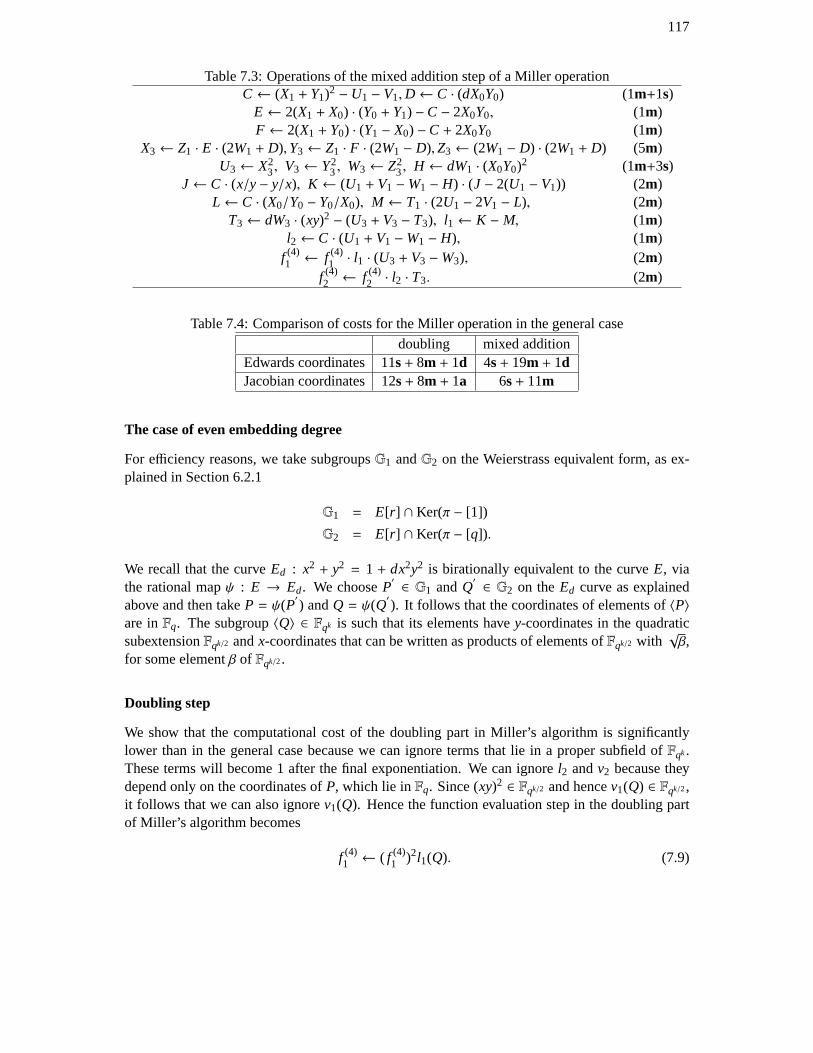
117

Table 7.3: Operations of the mixed addition step of a Miller operationC← (X1 + Y1)2 − U1 − V1,D← C · (dX0Y0) (1m+1s)

E← 2(X1 + X0) · (Y0 + Y1) −C − 2X0Y0, (1m)F ← 2(X1 + Y0) · (Y1 − X0) −C + 2X0Y0 (1m)

X3← Z1 · E · (2W1 + D),Y3← Z1 · F · (2W1 − D),Z3← (2W1 − D) · (2W1 + D) (5m)U3← X2

3, V3← Y23 , W3← Z2

3, H ← dW1 · (X0Y0)2 (1m+3s)J← C · (x/y− y/x), K ← (U1 + V1 −W1 − H) · (J − 2(U1 − V1)) (2m)

L← C · (X0/Y0 − Y0/X0), M ← T1 · (2U1 − 2V1 − L), (2m)T3← dW3 · (xy)2 − (U3 + V3 − T3), l1← K − M, (1m)

l2← C · (U1 + V1 −W1 − H), (1m)f (4)1 ← f (4)

1 · l1 · (U3 + V3 −W3), (2m)f (4)2 ← f (4)

2 · l2 · T3. (2m)

Table 7.4: Comparison of costs for the Miller operation in the general case

doubling mixed additionEdwards coordinates 11s+ 8m + 1d 4s+ 19m + 1dJacobian coordinates12s+ 8m + 1a 6s+ 11m

The case of even embedding degree

For efficiency reasons, we take subgroupsG1 andG2 on the Weierstrass equivalent form, as ex-plained in Section 6.2.1

G1 = E[r] ∩ Ker(π − [1])

G2 = E[r] ∩ Ker(π − [q]).

We recall that the curveEd : x2 + y2 = 1 + dx2y2 is birationally equivalent to the curveE, viathe rational mapψ : E → Ed. We chooseP

′ ∈ G1 andQ′ ∈ G2 on theEd curve as explained

above and then takeP = ψ(P′) andQ = ψ(Q

′). It follows that the coordinates of elements of〈P〉

are inFq. The subgroup〈Q〉 ∈ Fqk is such that its elements havey-coordinates in the quadraticsubextensionFqk/2 andx-coordinates that can be written as products of elements ofFqk/2 with

√β,

for some elementβ of Fqk/2.

Doubling step

We show that the computational cost of the doubling part in Miller’s algorithm issignificantlylower than in the general case because we can ignore terms that lie in a proper subfield ofFqk.These terms will become 1 after the final exponentiation. We can ignorel2 andv2 because theydepend only on the coordinates ofP, which lie inFq. Since (xy)2 ∈ Fqk/2 and hencev1(Q) ∈ Fqk/2,it follows that we can also ignorev1(Q). Hence the function evaluation step in the doubling partof Miller’s algorithm becomes

f (4)1 ← ( f (4)

1 )2l1(Q). (7.9)

118

Note that multiplications by (xy)2 and x/y − y/x cost (k/2)m each (x/y − y/x is the product ofsome element inFqk/2 with

√β). Also note that computingx/y− y/x once at the beginning costs

one inversion inFqk/2. In some protocolsQ is a fixed point, so we can precomputex/y− y/x.If k = 2, we actually have (xy)2 ∈ Fq and we computel1 as

l1(x, y) = ((X21 + Y2

1 − Z21)(X2

1 − Y21)) · 2X1Y1(x/y− y/x) − ((X2

1 + Y21 − Z2

1)

·(X21 − Y2

1)) · 2(X21 − Y2

1) − Z3 · (dZ21 · (xy)2 − (X2

1 + Y21 − Z2

1)),

For k > 2 some operations are done inFqk and others inFq, hence we computel1 as

l1(x, y) = ((X21 + Y2

1 − Z21)(X2

1 − Y21)) · 2X1Y1(x/y− y/x) − ((X2

1 + Y21 − Z2

1)

·(X21 − Y2

1)) · 2(X21 − Y2

1) − Z3 · dZ21 · (xy)2 + Z3 · (X2

1 + Y21 − Z2

1),

Computations do not differ much from those in Table 7.2 and we do not detail them. Results aresummarized in Table 7.5.

Table 7.5: Comparison of costs for the doubling step of the Miller operation in the case ofk even

k = 2 k ≥ 4Jacobian coordinates 10s+ 3m + 1a+ S+M 11s+ (k+ 1)m + 1a+ S+M

Das/Sarkar Edwards coordinates6s+ 9m + S+M -

(supersingular curves)Das/Sarkar Edwards inverted

6s+ 9m + S+M -coordinates (supersingular curves)

Edwards coordinates 4s+ 9m + 1d + S+M 4s+ (k+ 8)m + 1d + S+M

Mixed addition

Following a similar technique as the one for the doubling case, we obtain the mixedaddition stepfor evenk

f (4)1 ← ( f (4)

1 )2l1(Q). (7.10)

The detailed computations are similar to those in Table 7.3. Since computingX0Y0− Y0

X0costs one

inversion inFq, in some cases it will be less expensive to work withl′1 = (X0Y0)l1 instead ofl1.

For protocols in whichQ is a fixed point, we may precomputexy −

yx. This would give an inversion

free algorithm. Results and performance comparison are summarized Table 7.6.

Comparison

By looking at tables 7.5 and 7.6, one can see that in the case of curves with even embedding degreethe cost of an implementation of Miller’s algorithm in Edwards coordinates will beslightly moreexpensive than an implementation in Jacobian coordinates. We also checkedperformances of ourmethod in inverted Edwards coordinates, but we did not obtain better results. We underline theidea that, independently of the representation of curves and points chosen in an implementation

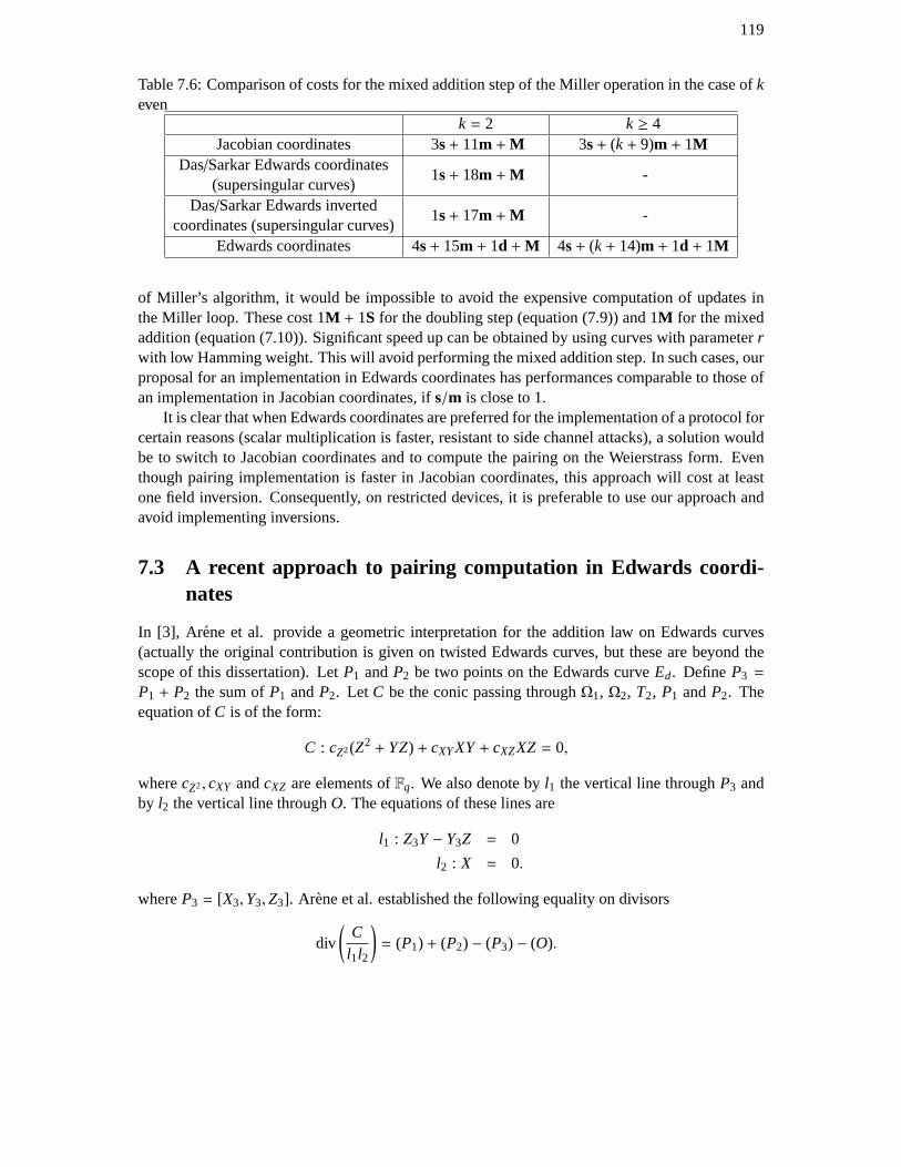
119

Table 7.6: Comparison of costs for the mixed addition step of the Miller operationin the case ofkeven

k = 2 k ≥ 4Jacobian coordinates 3s+ 11m +M 3s+ (k+ 9)m + 1M

Das/Sarkar Edwards coordinates1s+ 18m +M -

(supersingular curves)Das/Sarkar Edwards inverted

1s+ 17m +M -coordinates (supersingular curves)

Edwards coordinates 4s+ 15m + 1d +M 4s+ (k+ 14)m + 1d + 1M

of Miller’s algorithm, it would be impossible to avoid the expensive computation ofupdates inthe Miller loop. These cost 1M + 1S for the doubling step (equation (7.9)) and 1M for the mixedaddition (equation (7.10)). Significant speed up can be obtained by usingcurves with parameterrwith low Hamming weight. This will avoid performing the mixed addition step. In such cases, ourproposal for an implementation in Edwards coordinates has performancescomparable to those ofan implementation in Jacobian coordinates, ifs/m is close to 1.

It is clear that when Edwards coordinates are preferred for the implementation of a protocol forcertain reasons (scalar multiplication is faster, resistant to side channel attacks), a solution wouldbe to switch to Jacobian coordinates and to compute the pairing on the Weierstrass form. Eventhough pairing implementation is faster in Jacobian coordinates, this approachwill cost at leastone field inversion. Consequently, on restricted devices, it is preferable to use our approach andavoid implementing inversions.

7.3 A recent approach to pairing computation in Edwards coordi-nates

In [3], Arene et al. provide a geometric interpretation for the addition law on Edwards curves(actually the original contribution is given on twisted Edwards curves, butthese are beyond thescope of this dissertation). LetP1 andP2 be two points on the Edwards curveEd. DefineP3 =

P1 + P2 the sum ofP1 andP2. Let C be the conic passing throughΩ1, Ω2, T2, P1 andP2. Theequation ofC is of the form:

C : cZ2(Z2 + YZ) + cXYXY+ cXZXZ = 0,

wherecZ2, cXY andcXZ are elements ofFq. We also denote byl1 the vertical line throughP3 andby l2 the vertical line throughO. The equations of these lines are

l1 : Z3Y− Y3Z = 0

l2 : X = 0.

whereP3 = [X3,Y3,Z3]. Arene et al. established the following equality on divisors

div

(C

l1l2

)= (P1) + (P2) − (P3) − (O).

120

Table 7.7: Comparison of costs for the mixed addition step of the Miller operationin the case ofevenk

doubling mixed additionE [50] 4s+ (8+ k)m + 1d + 1S+ 1M 4s+ (k+ 14)m + 1d + 1ME [3] 5s+ 6m + 1S+ 1M (12+ k)m + 1M

J [50] [3] 11s+ (1+ k)m + 1a+ 1S+ 1M 6s+(6+k)m+1MJ ,y2 = x3 + b

(2k/e+2)m+7s+1a+1M+1S (2k/e+9)m+2s+1Me= 2,6 [23]J , y2 = x3 + ax

(2k/e+2)m+8s+1a+ 1M+1S (2k/e+12)m+4s+1Me= 2,4 [23]

This gives the Miller equation on the Edwards curve and, consequently, an efficient algorithm forpairing computation. We present in Table 7.7 the cost of their algorithm, in terms of the numberof operation in the doubling and the mixed addition steps of the Miller loop, in the case of curveswith even embedding degree. The casek = 1 is not evaluated in their paper.

To sum up, the Algorithm in [3] for pairing computation in Edwards coordinates is faster thanthen the method described in Section 7.2.3. However, ifs = 0.8m, a simple computation showsthat pairing computation is still fastest in Jacobian coordinates. Otherwise, whens/m is close to1, Edwards coordinates are to be preferred. Moreover, in the case of curves allowing twists ofdegree 4 or 6, it is not known whether we can represent the points inG2 as points overFqk/e, inorder to save multiplications.

7.4 An algorithm for scalar multiplication on incomplete Edwardscurves

SupposeEd is an Edwards curve overFq given by the equation

x2 + y2 = 1+ d(xy)2,

with d a square inFq. As explained in Section 7.1, this curve is notcomplete, i.e. the Edwardsaddition law is not complete. We denote byα a square root of 1/d. We consider the map:

τ : Ed → Ed

[x, y,1] 7→ [α

x,α

y,1]. (7.11)

One can easily check thatτ([x, y,1]) is a point on the Edwards curve. On special points we extendthis map as follows:

τ[0,1,1] = [1,0,0] andτ[1,0,0] = [0,1,1]

τ[1,0,1] = [0,1,0] andτ[0,1,0] = [1,0,1]

We show that the mapτ is in fact a translation map by a point of order 2, with respect to theaddition law on the elliptic curve.

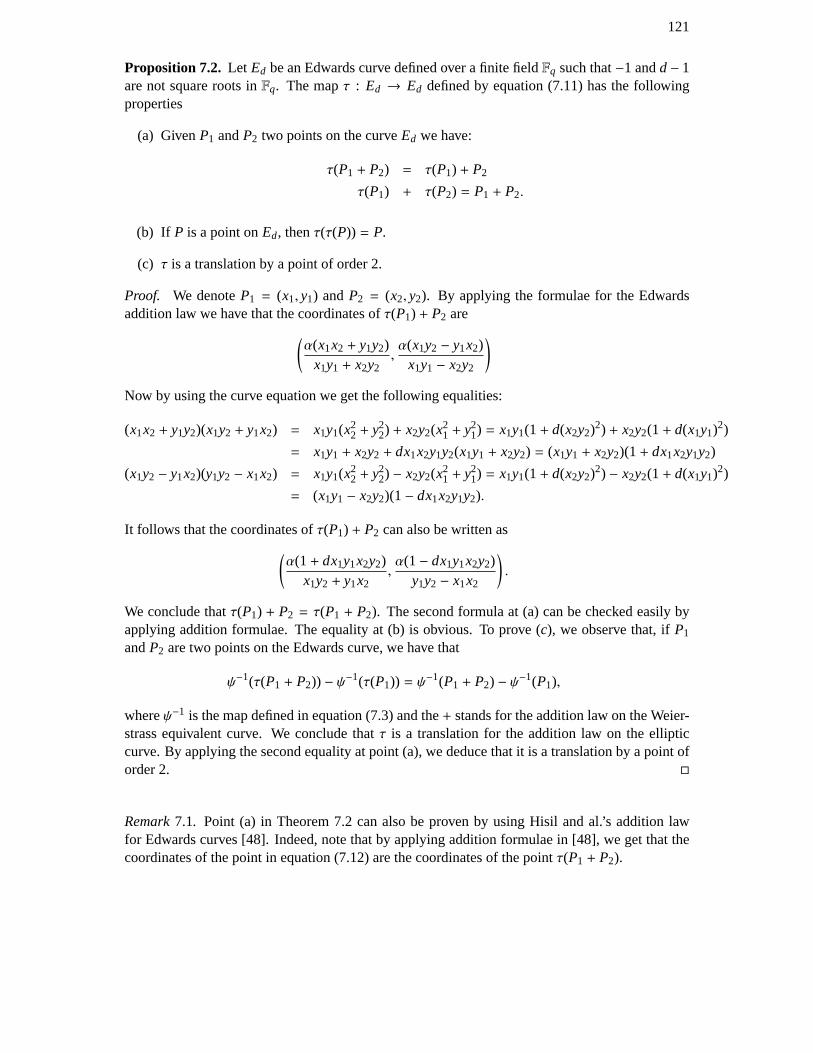
121

Proposition 7.2. Let Ed be an Edwards curve defined over a finite fieldFq such that−1 andd− 1are not square roots inFq. The mapτ : Ed → Ed defined by equation (7.11) has the followingproperties

(a) GivenP1 andP2 two points on the curveEd we have:

τ(P1 + P2) = τ(P1) + P2

τ(P1) + τ(P2) = P1 + P2.

(b) If P is a point onEd, thenτ(τ(P)) = P.

(c) τ is a translation by a point of order 2.

Proof. We denoteP1 = (x1, y1) andP2 = (x2, y2). By applying the formulae for the Edwardsaddition law we have that the coordinates ofτ(P1) + P2 are

(α(x1x2 + y1y2)

x1y1 + x2y2,α(x1y2 − y1x2)

x1y1 − x2y2

)

Now by using the curve equation we get the following equalities:

(x1x2 + y1y2)(x1y2 + y1x2) = x1y1(x22 + y2

2) + x2y2(x21 + y2

1) = x1y1(1+ d(x2y2)2) + x2y2(1+ d(x1y1)2)

= x1y1 + x2y2 + dx1x2y1y2(x1y1 + x2y2) = (x1y1 + x2y2)(1+ dx1x2y1y2)

(x1y2 − y1x2)(y1y2 − x1x2) = x1y1(x22 + y2

2) − x2y2(x21 + y2

1) = x1y1(1+ d(x2y2)2) − x2y2(1+ d(x1y1)2)

= (x1y1 − x2y2)(1− dx1x2y1y2).

It follows that the coordinates ofτ(P1) + P2 can also be written as

(α(1+ dx1y1x2y2)

x1y2 + y1x2,α(1− dx1y1x2y2)

y1y2 − x1x2

).

We conclude thatτ(P1) + P2 = τ(P1 + P2). The second formula at (a) can be checked easily byapplying addition formulae. The equality at (b) is obvious. To prove (c), we observe that, ifP1

andP2 are two points on the Edwards curve, we have that

ψ−1(τ(P1 + P2)) − ψ−1(τ(P1)) = ψ−1(P1 + P2) − ψ−1(P1),

whereψ−1 is the map defined in equation (7.3) and the+ stands for the addition law on the Weier-strass equivalent curve. We conclude thatτ is a translation for the addition law on the ellipticcurve. By applying the second equality at point (a), we deduce that it is atranslation by a point oforder 2.

Remark7.1. Point (a) in Theorem 7.2 can also be proven by using Hisil and al.’s addition lawfor Edwards curves [48]. Indeed, note that by applying addition formulae in [48], we get that thecoordinates of the point in equation (7.12) are the coordinates of the pointτ(P1 + P2).

122

Algorithm 13 Scalar multiplication on incomplete Edwards curvesINPUT: An Edwards curveEd/Fq, with d a square root inFq, a pointP on E andλ ∈ Z.OUTPUT: The pointλP.

1: Let i = [log2(λ)], K ← P, f ← 1, l ← 0.2: while i ≥ 1 do3: if 2K is definedthen4: K ← 2K5: end if6: elseK ← τ(K) + K; l ← l + 1.7: if the i-th bit of λ is 1 then8: if K + P is definedthen9: K ← K + P.

10: end if11: elseK ← τ(K) + P; l ← l + 1.12: end if13: end while14: if l mod 2 = 1 then15: K ← τ(K).16: end if17: return K.

The correctness of Algorithm 13 is transparent from Proposition 7.2. The conditions that−1andd − 1 are not squares ensure that whenever the Edwards additionP1 + P2 is not defined, themodified additionτ(P1) + P2 is defined (we no longer detail the computations). Hence Algo-rithm 13 works for all points on the curve. The algorithm is based on the square-and-multiplymethod, hence its complexity isO(logλ) in time. The cost of an addition of two points during theprocess is of 10m + 1s+ 1d, if performed in projective coordinates. We now evaluate the cost ofperforming the additionτ(P1) + P2, instead ofP1 + P2.

SupposeP1 = (X1,Y1,Z1) and P2 = (X2,Y2,Z2) two points we want to add. In projectivecoordinates, the formulae for computingτ(P1) + P2 are as follows

X3 = α(Z21Z2

2 + dX1X2Y1Y2)(Y1Y2 − X1X2)

Y3 = α(Z21Z2

2 − dX1X2Y1Y2)(X1Y2 + Y1X2)

Z3 = Z1Z2(X1Y2 + Y1X2)(Y1Y2 − X1X2)

This computation is performed as shown in Table 7.8. The operation count gives 9m+1s+1d+2αfor one addition. This is faster than addition in projective coordinates and as fast as addition ininverted Edwards coordinates.

Table 7.8: Complete addition for incomplete Edwards curvesA← Z1 · Z2, B← A2, C← X1 · X2, D← Y1 · Y2 (1s+3m)

E← dC · D, F ← B− E, G← B+ E, X3← α ·G · (D −C), H ← (X1 + Y1) · (X2 + Y2) −C − D (3m)Y3← α · F · H, Z3← A · H · (D −C) (3m)

We have given an efficient algorithm for scalar multiplication for Edwards curves whose addi-

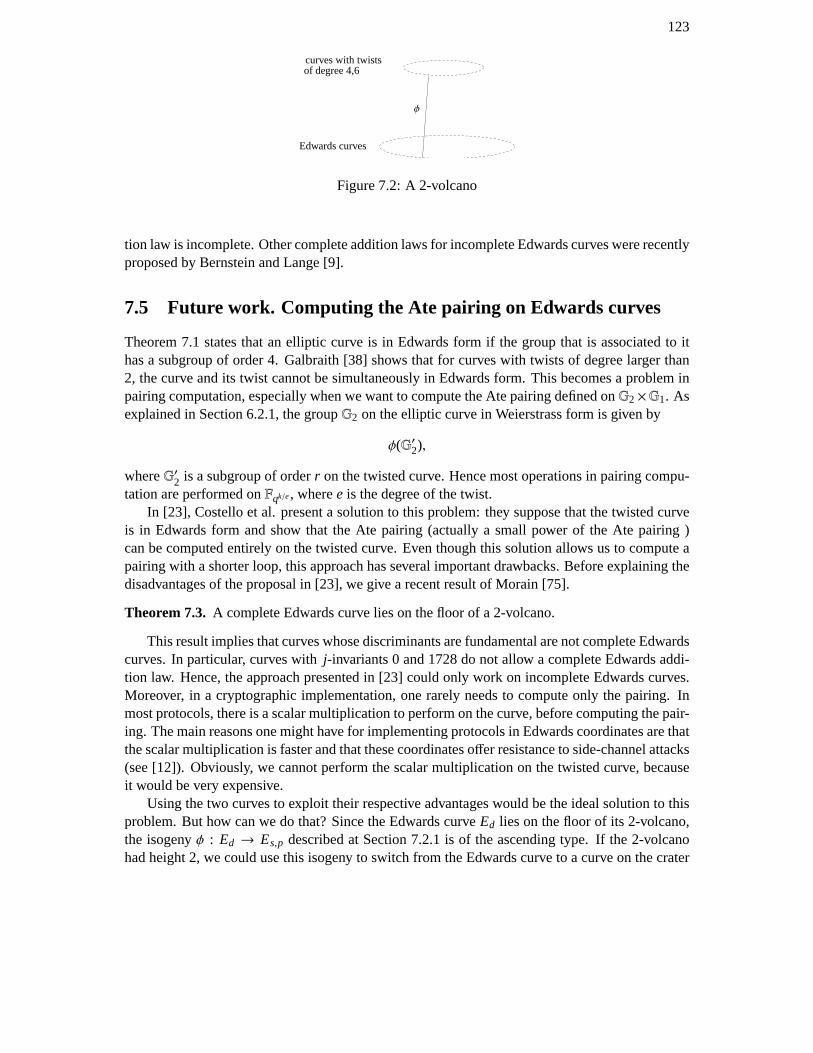
123

Edwards curves

curves with twistsof degree 4,6

φ

Figure 7.2: A 2-volcano

tion law is incomplete. Other complete addition laws for incomplete Edwards curveswere recentlyproposed by Bernstein and Lange [9].

7.5 Future work. Computing the Ate pairing on Edwards curves

Theorem 7.1 states that an elliptic curve is in Edwards form if the group that isassociated to ithas a subgroup of order 4. Galbraith [38] shows that for curves with twists of degree larger than2, the curve and its twist cannot be simultaneously in Edwards form. This becomes a problem inpairing computation, especially when we want to compute the Ate pairing definedonG2×G1. Asexplained in Section 6.2.1, the groupG2 on the elliptic curve in Weierstrass form is given by

φ(G′2),

whereG′2 is a subgroup of orderr on the twisted curve. Hence most operations in pairing compu-tation are performed onFqk/e, wheree is the degree of the twist.

In [23], Costello et al. present a solution to this problem: they suppose thatthe twisted curveis in Edwards form and show that the Ate pairing (actually a small power of theAte pairing )can be computed entirely on the twisted curve. Even though this solution allows us to compute apairing with a shorter loop, this approach has several important drawbacks. Before explaining thedisadvantages of the proposal in [23], we give a recent result of Morain [75].

Theorem 7.3. A complete Edwards curve lies on the floor of a 2-volcano.

This result implies that curves whose discriminants are fundamental are notcomplete Edwardscurves. In particular, curves withj-invariants 0 and 1728 do not allow a complete Edwards addi-tion law. Hence, the approach presented in [23] could only work on incomplete Edwards curves.Moreover, in a cryptographic implementation, one rarely needs to compute only the pairing. Inmost protocols, there is a scalar multiplication to perform on the curve, before computing the pair-ing. The main reasons one might have for implementing protocols in Edwards coordinates are thatthe scalar multiplication is faster and that these coordinates offer resistance to side-channel attacks(see [12]). Obviously, we cannot perform the scalar multiplication on the twisted curve, becauseit would be very expensive.

Using the two curves to exploit their respective advantages would be the ideal solution to thisproblem. But how can we do that? Since the Edwards curveEd lies on the floor of its 2-volcano,the isogenyφ : Ed → Es,p described at Section 7.2.1 is of the ascending type. If the 2-volcanohad height 2, we could use this isogeny to switch from the Edwards curve toa curve on the crater

124

of the volcano. However, this approach implies performing some inversionsin the finite field. Wehave found another isogeny of degree 4 from the Edwards curve to a curve in Weierstrass form,whose equation gives a method to switch between the two representations without performinginversions. We define the following isogeny from an Edwards curveEd to the curveE′s,p ofequationE′s,p : s2 = d2p3 + 2(d − 2)p2 + p

ϕ : Ed → E′s,p

(x, y) 7→ (xy(x2 − y2), (xy)2)

Suppose that3√d ∈ Fq. Then we substitute (s, p) for (s, p

3√d2

). We obtain a new equation for the

curveE′s,p:

s2 = p3 +2(d − 2)

d3√d

p2 +p

3√d2.

The kernel ofϕ is the 4-torsion subgroupO,T2,T4,−T4. It follows thatϕ is not a new isogeny,the curveE′s,p being actually isomorphic toEs,p.

Remark7.2. We have tried to useϕ to give an algorithm computing a 4-th power of the Tatepairing, using similar techniques to those in Section 7.2.3. Unfortunately, we have obtained analgorithm which is slower than the one in Section 7.2.3.

We believe that this isogeny may be the solution to efficiently computing the Ate pairing inEdwards coordinates on curves with discriminants−4 and−3. Moreover, this could also representa solution to the problem of using twists of high degree to compute the Tate pairing. Furtherinvestigation is needed to make sure we can actually employ the twists in these algorithms.

7.6 Conclusion

Efficiently implementing pairings on Edwards curves is a difficult problem. Some questions inthis research area remain open. For example, it is not possible to implement protocols using theAte pairing entirely in Edwards coordinates. Moreover, many families of pairing friendly curvescannot be given in Edwards form, because they do not fulfill the condition on the curve grouporder.

Chapter 8

Conclusion

At a first glance, this thesis treats two different subjects. The first one is a study of isogeny volca-noes using pairings, while the second one refers to the efficient implementation of cryptographicpairings using isogenies. In fact, the starting idea of our work is the following observation. GivenP andQ two ℓ-torsion points on the elliptic curve, the value of the pairingeℓ(P,Q) and an isogenyI : E→ E′, we have

eℓ(φ(P), φ(Q)) = eℓ(P,Q)degφ.

Part two of this dissertation relates this result to the isogeny classEllt(Fq). To every curveEin Ellt(Fq) we associate a quadratic formPE,ℓn2 which is an invariant of the set of curves havingthe same endomorphism ring asE. We show that the zeros of this quadratic form correspond topoints of orderℓ generating the kernel of horizontal or vertical isogenies in theℓ-isogeny volcanoof E. The remaining points of orderℓ generate the kernels of descending isogenies.

This discovery has important consequences on algorithms used to travel on the isogeny vol-cano. First of all, by evaluating the number of zeros of the quadratic formPE,ℓn2 , we give a methodto decide whether the curveE is on the crater of theℓ-volcano or not. Secondly, we give a methodto decide in advance, when taking a step on the volcano, whether this step is horizontal or de-scending, ascending or descending. Our method is very efficient, because it involves only thecomputation of a small number of pairings. The immediate consequence is that wehave foundvery simple algorithms, allowing to travel on the graph from one point to another.

In the third part, the approach is completely different. This time our goal is to make use ofthe isogeny in order to speed up the computation of the pairing valuee(P,Q). A first result isobtained by considering endomorphisms of small degree for pairing friendly elliptic curves. En-domorphisms were already used before in pairing computation [83] [47] [96]. However, until now,only endomorphisms with trivial kernel, such as the Frobenius endomorphism or automorphisms,were proposed. We propose endomorphisms having a kernel of small order. This gives a smallcorrection factor in the computation of the pairing, but the cost of the computation of this fac-tor is negligible. Our algorithm has better performances than Miller’s algorithmfor curves withembedding degree 2,3 and 4.

The second contribution in this area is an efficient algorithm to compute pairings on Edwardscurves. We used an isogeny of degree 4 between the Edwards curve and another curve of genus 1and derived formulae for efficient pairing computation on the Edwards curve.

125

126

8.1 Limitations of our methods and open problems

Isogeny volcanoes.Unfortunately, on some volcanoes, our method for determining the directionof an isogeny is very expensive in the upper part of the volcano, above the second stability level.Given a curveE lying on a level above the second stability level, all self-pairings ofℓ-torsionpoints ofE/Fq may be degenerate. Consequently, if we restrain to the volcano defined over thebase field, we cannot distinguish between a point spanning the kernel ofan horizontal isogenyfrom the point spanning the kernel of a descending isogeny, or the pointspanning the kernel ofthe ascending isogeny from the point spanning the kernel of the descending isogeny. However,we have shown that by considering the curve defined over an extensionfield Fq, with degree amultiple of ℓ, we find non-degenerate self-pairings ofℓ-torsion points. The only problem is thatcomputing these pairings may be very expensive, and the algorithms derived in this way will behighly inefficient. The question of how to predict directions of isogenies in the irregularpart ofthe volcano remains thus open. We only note that the non-degenerate pairings obtained over theextension fieldFqsℓ have values over the base fieldFq. This rises the question whether it would bepossible to compute these pairings more efficiently.

Isogeny volcanoes and cryptography.In Section 5.5.1, we presented a volcano-based algorithmto compute the Hilbert polynomial. Apart from the theoretical importance of this computation,advances in this area also have quickly found application in cryptography. Interest in algorithmsallowing to compute this polynomial has arisen because of the key role this polynomial plays inmethods to construct pairing friendly curves.

As explained in section 6.1, some families of pairing friendly curves are veryrare, and findingcurves in such families depends drastically on our ability to computeHD(X) for large discriminantsD. We explain this idea by an example. For MNT curves with embedding degree 6,Sutherland’scomputations [89] gave 500 discriminantsD, with D < 1012 which provide pairing friendly curvesat 80 bits security level (according to [36]).

Consequently, a logical continuation of the work in this thesis would be to adapt Sutherland’salgorithm to our methods and see whether this results into obtaining the class equations for largerdiscriminants.

The same considerations are valid for the algorithm computing modular polynomials[90],which are needed in cryptography since certain algorithms (such as Schoof’s algorithm) use pre-computations of this polynomial.

Cryptographic non-degenerate self pairings.We explained in Chapter 6 that non-degenerateself-pairings have many cryptographic applications. While on supersingular curves, constructingsuch pairings is rather easy thanks to distortion maps, on ordinary curvesmatters are more compli-cated. In Section 6.4 we have given a method to construct ordinary curves having non-degenerateself-pairings for all points of orderr. Our construction is the first construction of this kind whichdoes not use distortion maps.

The curves have embedding degree 1 andρ-value is approximately 2. Unfortunately, becauseof the highρ-value, we estimate that pairing computation is less efficient on these curves than onsupersingular curves with embedding degree 2. The questions of how to implement these pairingsefficiently and how to hash to these curves efficiently remain open.

127

Pairing implementation using endomorphisms. In Chapter 6 we have given a method to useendomorphisms to speed up pairing computation on curves with small discriminant.We havesurveyed many existing constructions of pairing friendly curves with small discriminant to seewhether our method applies to these constructions. More precisely, we were interested in findingcurves for which the size of the eigenvalueλ of the endomorphism is approximately

√r. We have

found that our method works on curves constructed with the Cocks-Pinchmethod, which is veryflexible in choosing the value ofr. Unfortunately, because of the high value of the parameterρ,these curves are far from being optimal for pairing based cryptography. We raise the questionwhether it would be possible to construct by complex multiplication curves having eigenvaluesλ ≈√

r and betterρ-value.

Pairing on Edwards curves. We have given an isogeny of degree 4 from the Edwards curve toa curve in Weierstrass form. F. Morain [75] showed recently that completeEdwards curves lieon the floor of 2-volcanoes. This result implies that on a 4-volcano, our isogeny is ascending. Inthe case of curves with discriminant−4 and−3 lying on a 2-volcano of height 2, this allows usto transport points from the Edwards curve lying on the floor to a curve lying on the crater. Thisgives an inversion free algorithm to compute the Ate pairing on the Weierstrass curve, by makinguse of twists of degree 4 and 6. However, we do not know whether it is possible, by using theisogeny or its dual, to find an algorithm which computes the Ate pairing (or a smallpower of theAte pairing) entirely in the Edwards form.

Bibliography

[1] T. Okamoto A. Menezes and S.A. Vanstone. Reducing elliptic curve logarithms to logarithmsin the finite field. InProceedings 23rd Annual ACM Symposium on Theory of Computing(STOC), pages 80–89. ACM Press, 1991.

[2] L.M. Adleman, J. DeMarrais, and M.-D. Huang. A subexponential algorithm for discretelogarithms over hyperelliptic curves of large genus over GF (q).Theoretical Computer Sci-ence, 226(1-2):7–18, 1999.

[3] C. Arene, T. Lange, M. Naehrig, and C. Ritzenthaler. Faster Computation of theTate Pairing.http://eprint.iacr.org/2009/155.

[4] M. Atiyah and I. Macdonald.Introduction to Commutative Algebra. Addison-Wesley, 1969.

[5] A.O.L. Atkin. The number of points on an elliptic curve modulo a prime. E-mail on theNumber Theory Mailing List, 1988.

[6] P. Barreto, S. Galbraith, C. Heigeartaigh, and M. Scott. Efficient Pairing Computation onSupersingular Abelian Varieties.Des. Codes Cryptography, 42(3):239–271, 2007.

[7] P. Barreto and M. Naehrig. Pairing-friendly elliptic curves of prime order. In B. Preneel andS. Tavares, editors,Selected Areas in Cryptography - SAC 2005, volume 3897 ofLectureNotes in Computer Science, pages 319 –331. Springer, 2006.

[8] J. Belding, R. Broker, A. Enge, and K. Lauter. Computing Hilbert class polynomials. In A.J.van der Poorten and A. Stein, editors,Algorithmic Number Theory Symposium-ANTS VIII,volume 5011 ofLecture Notes in Computer Science, pages 282–295. Springer Verlag, 2008.

[9] D. Bernstein and T. Lange. A complete set of addition laws for incompleteEdwards curves.http://eprint.iacr.org/2009/580.

[10] D. Bernstein and T. Lange. Explicit formulas-database. http://www.hyperelliptic.org/EFD,2007.

[11] D. J. Bernstein, P. Birkner, M. Joye, T. Lange, and C. Peters.Twisted Edwards curves. InS. Vaudenay, editor,AFRICACRYPT, volume 5023 ofLecture Notes in Computer Science,pages 389–405. Springer Verlag, 2008.

129

130

[12] D. J. Bernstein and T. Lange. Faster addition and doubling on elliptic curves. In K. Kuro-sawa, editor,Advances in Cryptology – ASIACRYPT 2007, volume 4833 ofLecture Notes inComputer Science, pages 29–50. Springer Verlag, 2007.

[13] D. J. Bernstein and T. Lange. Inverted Edwards coordinates. In S. Boztas and H.F. Lu,editors,AAECC 2007, volume 4851 ofLecture Notes in Computer Science, pages 20–27.Springer Verlag, 2007.

[14] G. Bisson and A. Sutherland. Computing the endomorphism ring of an ordinary ellipticcurve over a finite field. http://eprint.iacr.org/2009/100, 2009.

[15] I. F. Blake, G. Seroussi, and N. P. Smart.Advances in Elliptic Curve Cryptography, volume317 of London Mathematical Society Lecture Note Series. Cambridge University Press,2005.

[16] D. Boneh and M. K. Franklin. Identity-based encryption from the Weil pairing. In J. Kilian,editor,Advances in Cryptology – CRYPTO 2001, volume 2139 ofLecture Notes in ComputerScience, pages 213–229. Springer Verlag, 2001.

[17] D. Boneh, B. Lynn, and H. Shacham. Short signatures from the Weil pairing. In C. Boyd,editor,Advances in Cryptology – ASIACRYPT 2001, volume 2248 ofLecture Notes in Com-puter Science, pages 514–532. Springer Verlag, 2001.

[18] D. Boneh, K. Rubin, and A. Silverberg. Finding composite order ordinary elliptic curvesusing the Cocks-Pinch method. to appear in Journal of Number Theory.

[19] Z.I. Borevitch and I.R. Chafarevitch.Theorie des nombres. Gauthiers-Villars, Paris, 1967.

[20] F. Brezing and A. Weng. Elliptic curves suitable for pairing based cryptography.Des CodesCryptography, 37(1):133–141, 2005.

[21] R. Broker.Constructing elliptic curves of prescribed order. PhD thesis, Universiteit Leiden,2006.

[22] R. Broker and P. Stevenhagen. Constructing elliptic curves of primeorder. ContemporaryMathematics, (463):17–28, 2008.

[23] T. Lange C. Costello and M. Naehrig. Faster Pairing Computations on Curves with High-Degree Twists. In P. Q. Nguyen and D. Pointcheval, editors,Public Key Cryptography-PKC2010, Lecture Notes in Computer Science, pages 224–242. Springer, 2010.

[24] D. Charles. On the existence of distortion maps on ordinary curves.http://eprint.iacr.org/2006/128.

[25] D. A. Cox. Primes of the Form x2 + ny2: Fermat, class field theory, and complex multiplica-tion. John Wiley & Sons, Inc, 1989.

[26] M. Prem Laxman Das and P. Sarkar. Pairing computation on twisted Edwards form ellipticcurves. In S. Galbraith and K. Paterson, editors,Pairing, volume 5209 ofLecture Notes inComputer Science, pages 192–210. Springer Verlag, 2008.

131

[27] M. Deuring.Die Typen der Multiplikatorenringe elliptischer Funktionenkorper. Abh. Math.Sem. Hansischen Univ. 14, 1941.

[28] L. Dewaghe. Un corollaire aux formules de Velu. Draft, 1995.

[29] C. Diem. The GHS attack in odd characteristic.Journal of Ramanujan Mathematical Society,18(1):1–32, 2003.

[30] W. Diffie and M. Hellman. New Directions in Cryptography.IEEE Transcations on Infor-matics Theory, IT-22(6):644–654, 1976.

[31] S. Duquesne and G. Frey. Background on pairings, Chapter 6.In Handbook of ellipticand hyperelliptic curve cryptography, pages 115–132. Chapman and Hall/CRC, Taylor andFrancis Group, 2006.

[32] H. M. Edwards. A normal form for elliptic curves.Bull. AMS, 44:393–422, 2007.

[33] N.D. Elkies. Explicit isogenies. Draft, 1991.

[34] M. Fouquet.Anneau d’endomorphismes et cardinalite des courbes elliptiques: aspects al-gorithmiques. PhD thesis, Ecole Polytechnique, 2001.

[35] M. Fouquet and F. Morain. Isogeny volcanoes and the SEA algorithm. In C. Fieker andD. R. Kohel, editors,ANTS-V, volume 2369 ofLecture Notes in Computer Science, pages276–291. Springer, 2002.

[36] D. Freeman, M. Scott, and E. Teske. A taxonomy of pairing-friendlyelliptic curves.Journalof Cryptology, (23):224–280, 2006.

[37] G. Frey and H.-G. Ruck. A remark concerningm-divisibility and the discrete logarithmproblem in the divisor class group of curves.Math.Comp., 62:865–874, 1994.

[38] S. Galbraith. Twists of Edwards curves. Draft, 2009.

[39] S. Galbraith, F. Hess, and N. Smart. Extending the GHS Weil-descentattack. In L. R. Knud-sen, editor,EUROCRYPT02, volume 2332 ofLecture Notes in Computer Science, pages29–44. Springer, 2002.

[40] S. Galbraith, J.F McKee, and P.C. Valenca. Ordinary abelian varieties having small embed-ding degree.Finite Fields and their Applications, (13):800–814, 2007.

[41] P. Gaudry. An algorithm for solving the discrete log probleme on hyperelliptic curves. InB. Preneel, editor,EUROCRYPT00, volume 1807 ofLecture Notes in Computer Science,pages 19–34. Springer, 2000.

[42] P. Gaudry, E. Thome, N. Theriault, and C. Diem. A double large prime variation for smallgenus hyperelliptic index calculus.Mathematics of Computation, 76(257):475–492, 2007.

[43] R. Granger, F. Hess, R. Oyono, N. Theriault, and F. Vercauteren. Ate pairing on hyperellipticcurves. In M. Naor, editor,EUROCRYPT07, Lecture Notes in Computer Science, pages 430–447. Springer, 2007.

132

[44] R. Granger, D. Page, and N. P. Smart. High security pairing-based cryptography revisited. InF. Hess, S. Pauli, and M. E. Pohst, editors,ANTS, volume 4076 ofLecture Notes in ComputerScience, pages 480–494, 2006.

[45] R. Hartshorne.Algebraic Geometry, volume 52 ofGraduate Texts in Mathematics. Springer,1977.

[46] F. Hess. A note on the Tate pairing of curves over finite fields.Arch. Math, 82:28–32, 2004.

[47] F. Hess, N. P. Smart, and F. Vercauteren. The Eta pairing revisited.IEEE Transactions onInformation Theory, 52:4595–4602, 2006.

[48] Huseyin Hisil, Kenneth Koon-Ho Wong, Gary Carter, and Ed Dawson. Twisted edwardscurves revisited. InASIACRYPT ’08: Proceedings of the 14th International Conferenceon the Theory and Application of Cryptology and Information Security, pages 326–343.Springer-Verlag, 2008.

[49] S. Ionica and A. Joux. Pairing the volcano. InAlgorithmic Number Theory. 9th InternationalSymposium, Nancy, France, ANTS-IX, July 19-23, 2010, Proceedings, To appear.

[50] S. Ionica and A. Joux. Another approach to pairing computation in Edwards coordinates.In D. R. Chowdhury, V. Rijmen, and A. Das, editors,Progress in Cryptography- Indocrypt2008, volume 5365 ofLecture Notes in Computer Science, pages 400–413. Springer, 2008.

[51] A. Joux. A one round protocol for tripartite Diffie-Hellman. Journal of Cryptology,17(4):263–276, September 2004.

[52] A. Joux and R. Lercier. The Function Field Sieve in the Medium Prime Case. InAdvancesin Cryptology: Eurocrypt 2006.

[53] A. Joux, R. Lercier, N. Smart, and F. Vercauteren. The Number Field Sieve in the MediumPrime Case. In Cynthia Dwork, editor,Advances in Cryptology- CRYPTO 2006, volume4117 ofLecture Notes in Computer Science, pages 326–344, 2006.

[54] A. Joux and K. Nguyen. Separating Decision Diffie Hellman from Computational DiffieHellman in Cryptographic Groups.Journal of Cryptology, 16(4):239–247, 2003.

[55] H.W. Lenstra Jr. Complex multiplication structure of elliptic curves.Journal of NumberTheory, 56(2):227–241, 1996.

[56] E. Kachisa, E. Schaefer, and M. Scott. Constructing Brezing-Weng pairing friendly ellipticcurves using elements in the cyclotomic field. In S. Galbraith and K. Paterson,editors,Pair-ing Based Cryptography-Pairing 2008, volume 5209 ofLecture Notes in Computer Science,pages 126–135, 2008.

[57] K. Karabina and E. Teske. On prime order elliptic curves with embedding degrees 3,4 and6. In A.J. van der Poorten and A. Stein, editors,Algorithmic Number Theory Symposium-ANTS-VIII, volume 5011 ofLecture Notes in Computer Science, pages 102–117. Springer,2008.

133

[58] N. Koblitz. Elliptic curve cryptosystems.Mathematics of Computation, 48(177):203–209,1987.

[59] N. Koblitz. Hyperelliptic curve cryptosystems.Journal of Cryptology, 1:139–150, 1989.

[60] N. Koblitz and A. Menezes. Pairing-based cryptography at high security levels. In N. P.Smart, editor,Proceedings of Cryptography and Coding 2005, volume 3796 ofLecture Notesin Computer Science, pages 13–36, 2005.

[61] D. Kohel. Endomorphism rings of elliptic curves over finite fields. PhD thesis, University ofCalifornia, Berkeley, 1996.

[62] S. Lang.Elliptic Functions, volume 112 ofGraduate Texts in Mathematics. Springer Verlag,1987.

[63] S. Lang.Algebraic Number Theory, volume 110 ofGraduate Texts in Mathematics. SpringerVerlag, 1994.

[64] R. Lercier. Algorithmique des Courbes Elliptiques dans les Corps Finis. PhD thesis,Ecolepolytechnique, Palaiseau, 1997.

[65] R. Lercier, D. Lubicz, and F. Vercauteren. Point counting on elliptic and hyperelliptic curves,Chapter 17. InHandbook of elliptic and hyperelliptic curve cryptography, pages 407–454.Chapman and Hall/CRC, Taylor and Francis Group, 2006.

[66] S. Lichtenbaum. Duality theorems for curves overp-adic fields.Invent.Math.7, pages 120–136, 1969.

[67] F. Luca and I. Shparlinski. Elliptic curves with small embedding degree. Journal of Cryp-tology, (19):553–562, 2006.

[68] MAGMA Computational Algebra System. MAGMA version V2.16-5, 2010.http://magma.maths.usyd.edu.au/magma.

[69] V. Miller. Use of elliptic curves in cryptography. In A. M. Odlyzko, editor, Advances inCryptology – CRYPTO’86, volume 263, pages 417–426. Springer Verlag, 1986.

[70] V. Miller. The Weil pairing, and its efficient calculation.Journal of Cryptology, 17(4):235–261, September 2004.

[71] J. Miret, R. Moreno, D. Sadornil, J. Tena, and M. Valls. An algorithm to compute volcanoesof 2-isogenies on elliptic curves over finite fields.Applied Mathematics and Computation,176(2):736–750, 2006.

[72] J. Miret, R. Moreno, D. Sadornil, J. Tena, and M. Valls. Computing the height of volcanoesof l-isogenies of elliptic curves over finite fields.Applied Mathematics and Computation,196(1):67–76, 2008.

[73] A. Miyaji, M. Nakabayashi, and S. Takano. New explicit of elliptic curve traces for FR-reduction.IEICE Transactions on Fundamentals, E84-A5(5):1234–1343, 2001.

134

[74] P.L. Montgomery.A FFT extension of the elliptic curve method of factorization. PhD thesis,University of California, 1992.

[75] F. Morain. Edwards curves and CM multiplication. http://hal.inria.fr/inria-00375427/fr.

[76] P.C.van Oorschot and M.J.Wiener. Parallel collision search with cryptanalytic applications.Journal of Cryptology, (12):1–18, 1999.

[77] The PARI Group, Bordeaux.PARI/GP, version 2.1.5, 2005. http://pari.math.u-bordeaux.fr.

[78] S. Pohlig and M. Hellmann. An improved algorithm for computing logarithms over GF(p)and its cryptographic significance.IEEE Transactions in Information Theory, IT-24:106–110, 1978.

[79] J. Pollard. Monte Carlo methods for index computation (modp). Mathematics of Computa-tion, (32):918–924, 1978.

[80] H.-G. Ruck. A note on elliptic curves over finite fields.Mathematics of Computation,179:301–304, 1987.

[81] T. Satoh and K. Araki. Fermat quotients and the polynomial time discrete log algorithm foranomalous curves.Comm. Math. Univ. Sancti Pauli, 47:81–92, 1998.

[82] R. Schoof. Counting points on elliptic curves over finite fields.Journal de Theorie desNombres de Bordeaux, 7:219–254, 1995.

[83] M. Scott. Faster pairings using an elliptic curve with an efficient endomorphism. In S. Maitra,C. E. V. Madhavan, and R. Venkatesen, editors,INDOCRYPT 2005, volume 3797 ofLectureNotes in Computer Science, pages 258–269. Springer, 2005.

[84] A. Shamir. Identity-based cryptosystems and signature schemes. InG. R. Blakley andD. Chaum, editors,CRYPTO84, volume 196 ofLecture Notes in Computer Science, pages47–53. Springer, 1985.

[85] D. Shanks. Class number, a theory of factorization, and genera.In Proceedings of Symposiumof Pure Mathematics, volume 20, pages 415–440. American Mathematical Society, 1971.

[86] J. H. Silverman.The Arithmetic of Elliptic Curves, volume 106 ofGraduate Texts in Mathe-matics. Springer, 1986.

[87] J.H. Silverman.Advanced Topics in the Arithmetic of Elliptic Curves, volume 151 ofGrad-uate Texts in Mathematics. Springer, 1994.

[88] A. Sutherland. Pairing-friendly curves suitable for cryptography. http://www-math.mit.edu/ drew/WeberModPolys.html.

[89] A. Sutherland. Pairing-friendly curves suitable for cryptography. http://www-math.mit.edu/ drew/MNTCurves.

[90] A. Sutherland. Modular polynomials via isogeny volcanoes. http://arxiv.org/abs/1001.0402,2009.

135

[91] Andrew Sutherland. Computing Hilbert Class Polynomials with the CRT.http://arxiv.org/abs/0903.2785, 2009.

[92] J. Tate. WC-groups overp-adic fields. InSeminaire Bourbaki; 10e annee: 1957/1958. Textesdes conferences;Exposes 152 a 168; 2e ed. corrigee,Expose 156, volume 13. Secretariatmathematique, Paris, 1958.

[93] J. Velu. Isogenies entre courbes elliptiques.Comptes Rendus De Academie Des SciencesParis, Serie I-Mathematique, Serie A., 273:238–241, 1971.

[94] E.R. Verheul. Evidence that XTR is more secure that supersingularelliptic curve cryptosys-tems. In B. Pfitzmann, editor,Advances in Cryptography: EUROCRYPT 2001, volume 2045of Lecture Notes in Computer Science, pages 195–201. Springer, 2001.

[95] J. von zur Gathen and V. Shoup. Computing Frobenius maps and factoring polynomials.Computational Complexity, 2:187–224, 1992.

[96] C. Zhao and F. Zhang. Computing the Bilinear Pairings on Elliptic Curveswith Automor-phisms. http://eprint.iacr.org/2008/209.

137

Resume

Les couplages sont utilises en cryptographie pour mener des attaques contre le logarithme discretsur certaines courbes elliptiques, ainsi que pour la construction des schemas cryptographiques.Depuis 2000, la cryptographiea base des couplages a connu un grand essor.

Dans cette these, nous nous interessons dans un premier tempsa l’implementation des cou-plages en utilisant des isogenies. Ces travaux incluent une methode pour le calcul du couplagesur des courbes elliptiques ayant des endomorphismes de petit degre. Nous proposons par ailleursun algorithme qui calcule le couplage sur la courbe d’Edwards,a l’aide d’une isogenie de degre 4entre la courbe d’Edwards et une autre courbe de genre 1.

Dans un deuxieme temps, nous proposons les couplages pour l’etude des volcans d’isogenies.Les volcans d’isogenies sont des graphes dont les noeuds sont des courbes elliptiques et les aretessont des l-isogenies entre les courbes. En 1996, Kohel propose l’utilisation du parcours en pro-fondeur de ces graphes dans un algorithme qui calcule l’anneau d’endomorphismes d’une courbeelliptique. Fouquet et Morain (2001) ont propose d’autres algorithmes pour le parcours de cesgraphes. Cependant, jusqu‘a present, il n’etait pas possible de predire la direction d’un pas sur levolcan; de fait, un grand nombre de pas successifsetait necessaire avant de determiner la directionprise. Nous introduisons une methode qui permet de calculer, pour une courbe elliptique E, lespoints d’ordre l qui engendrent les noyaux des isogenies descendantes, ascendantes ou horizon-tales. Notre methode, basee sur le calcul de quelques couplages, est tres efficace et donne, dansbeaucoup de cas, des algorithmes plus rapides que les methodes existantes pour le parcours desvolcans d’isogenies.

Abstract

Pairings are used in cryptography to attack the discrete logarithm problem on some curves andalso in building cryptosystems. Since 2000, pairing based cryptography has been an active area ofresearch.

In this thesis, we first study algorithms for pairing computation combined with isogenies. Wegive an algorithm for pairing computation using endomophisms of small degreeand an efficientimplementation of pairings on an Edwards curve, by making use of an isogenyof degree 4 betweenthe Edwards curve and another genus one curve.

Secondly, we propose pairings in the study of isogeny volcanoes. Isogeny volcanoes are graphswhose vertices are elliptic curves and whose edges are l-isogenies. Algorithms allowing to travelon these graphs were developed by Kohel in his thesis (1996) and later on, by Fouquet and Morain(2001). However, up to now, no method was known, to predict, before taking a step on the volcano,the direction of this step. To solve this issue, we develop a method to determine onan elliptic curvethe points of order l that generate kernels of descending, ascending and horizontal isogenies. Ourmethod, based on the computation of a few pairings, is very efficient and gives, in most cases,simple algorithms, allowing to either walk on the crater, descend from the craterto the floor orascend from the floor to the crater.

Algorithmique des couplages et cryptographie - Lix

Documents

Transcript of Algorithmique des couplages et cryptographie - Lix