Agreement strategies for multi-robot systems · 2015-01-21 · aleVntina, Wenjuan and Dung, for all...
232
THÈSE Pour obtenir le grade de DOCTEUR DE L’UNIVERSITÉ DE GRENOBLE Spécialité : Automatique et Productique Arrêté Ministériel : 7 août 2006 Présentée par Gabriel RODRIGUES DE CAMPOS Thèse dirigée par Carlos CANUDAS DE WIT et codirigée par Alexandre SEURET préparée au sein du laboratoire GIPSA-Lab, Département Automatique, du centre de recherche INRIA Grenoble Rhône-Alpes et de l’école doctorale Électronique, Électrotechnique, Automatique et Traitement du Signal Agreement strategies for multi-robot systems Stratégies de commande collaborative pour des systèmes multi-robots Thèse soutenue publiquement le 23 novembre 2012, devant le jury composé de : Mazen ALAMIR, Président Directeur de Recherche CNRS, GIPSA-Lab (Grenoble, France) António PASCOAL, Rapporteur Professeur, Instituto Superior Técnico (Lisbonne, Portugal) Christopher EDWARDS, Rapporteur Professeur, University of Leicester (Leicester, Angleterre) Sandra HIRCHE, Rapporteur Professeur, Technische Universität München (Munich, Allemagne) Dimos DIMAROGONAS, Examinateur Assistant Professor, Royal Institute of Technology (Stockholm, Suède) Alexandre SEURET, Codirecteur de thèse Chargé de Recherche CNRS, GIPSA-Lab (Grenoble, France)
Transcript of Agreement strategies for multi-robot systems · 2015-01-21 · aleVntina, Wenjuan and Dung, for all...
THÈSEPour obtenir le grade de
DOCTEUR DE L’UNIVERSITÉ DE GRENOBLESpécialité : Automatique et Productique
Arrêté Ministériel : 7 août 2006
Présentée par
Gabriel RODRIGUES DE CAMPOS
Thèse dirigée par Carlos CANUDAS DE WITet codirigée par Alexandre SEURET
préparée au sein du laboratoire GIPSA-Lab, Département Automatique,du centre de recherche INRIA Grenoble Rhône-Alpeset de l’école doctorale Électronique, Électrotechnique, Automatique etTraitement du Signal
Agreement strategies for multi-robotsystemsStratégies de commande collaborative pour des systèmesmulti-robots
Thèse soutenue publiquement le 23 novembre 2012,devant le jury composé de :
Mazen ALAMIR, PrésidentDirecteur de Recherche CNRS, GIPSA-Lab (Grenoble, France)António PASCOAL, RapporteurProfesseur, Instituto Superior Técnico (Lisbonne, Portugal)Christopher EDWARDS, RapporteurProfesseur, University of Leicester (Leicester, Angleterre)Sandra HIRCHE, RapporteurProfesseur, Technische Universität München (Munich, Allemagne)Dimos DIMAROGONAS, ExaminateurAssistant Professor, Royal Institute of Technology (Stockholm, Suède)Alexandre SEURET, Codirecteur de thèseChargé de Recherche CNRS, GIPSA-Lab (Grenoble, France)


This thesis received the European Label

No one can whistle a symphony.
It takes a whole orchestra to play it.
— H. E. Luccock


To my parents

Acknowledgments
First of all, I would like to thank all the members of my committee for their involve-ment, questions and feedback: to Prof. Mazen Alamir for accepting to be the committeepresident; to Prof. Antonio Pascoal, Prof. Christopher Edwards and Prof. SandraHirche for kindly accepting to review this document; to Dr. Dimos V. Dimaragonas, notonly for his guidance while staying at KTH but also for accepting to join us in Grenobleto participate at the discussion of this work. Their comments, observations, and sug-gestions greatly helped me to improve this thesis and their commitment was crucial forobtaining the European Label for this work.
I would like to thank my supervisor, Carlos Canudas de Wit, for the opportunityof joining the NeCS team. For his advice, support, and mostly for all the challengingpossibilities he oered me during this period, especially throughout the FeedNetBack andConnect projects and the international mobility period I enjoyed. I am also thankfulto my co-supervisor, Alexandre Seuret, for his trust and his encouraging guidance. Notonly I found his support to all my projects and aspirations but I could develop with himan unforgettable friendship.
I was fortunate enough to undertake some of the work for this thesis in Sweden, whereI spent an amazing six months at KTH. My gratitude goes to Prof. Karl H. Johanssonand Dr. Dimos V. Dimarogonas, who provide me with their precious help and guidanceand oered me the possibility of joining the Automatic Control Lab at KTH. This periodwas a particularly great experience for me, mainly because of all the wonderful peopleI had the chance to meet in Sweden. Finally, I also acknowledge Grenoble INP for thenancial support that made this research visit possible.
I am very grateful to Janan Zaytoon and Noureddine Manamanni, for their helpfulpresence during my studies at Reims and for my rst insight to academia and research,and to all the people that provide me with comments and suggestions regarding thisdocument, especially to Prof. Linda Simões.
During these three years, I met great people and shared amazing experiences atthe Gipsa- Lab. I would like to thank all its members, and in particular those from theDepartment of Automatic Control. Thank you to my oce colleagues and friends Emilie,
9

Valentina, Wenjuan and Dung, for all your daily smiles, jokes and support. Thank you toall PhD students and in particular to Nicolas, Lara B., and Augustin for their friendships,tips and all the cool moments.
Thank you to all the team members I had the pleasure to work with at the GipsADoc,especially to Antoine, Chloe, Emilie, Yo and Vincent. I also acknowledge Prof. Jean-Marc Thiriet and Dr. Nicolas Marchand for their support to student's initiatives ingeneral.
I am especially grateful to the people that shared my life during these three yearsand to my friends with who I lived so many adventures and experiences: Marco, Lara J.and Elsa for their unconditional friendship, all my "amis grenoblois" and all the friendsI had the chance to meet through conferences, meetings and projects.
I could not nish without mentioning my family, especially my brothers, who havealways stood by me. Finally, I would like to express my gratitude to my parents forsupporting me, my dreams and aspirations. This thesis is dedicated to them.
Lastly, I would like to thank everyone that, in a way or another, shared momentswith me and contribute to this accomplishment.
Gabriel Campos
Grenoble, 2012
10
Abstract
The idea of deploying formations of relatively unsophisticated autonomous robotsto accomplish complicated tasks has roots in the early works studying the ocking andforaging behaviors among birds. The main question was how one can mimic dierentbehaviors witnessed in populations of birds, animals, insects, etc. among a population ofarticial agents. The emerging use of large-scale multi-agent and multi-vehicle systemsin various modern applications has recently raised the need for the design of controllaws to perform challenging spatially-distributed tasks such as search and recovery op-erations, exploration, surveillance, environmental monitoring or pollution detection andestimation, among many others.
This dissertation focuses on distributed control strategies for a set of mobile robots,with a particular attention to agreement protocols. A signicant part of the manuscriptdeals with consensus algorithms of arbitrary linear heterogeneous agents, representing,for example, dierent models or generations of robots. Motivated by the fact that only afew works consider heterogeneous cases of the synchronization problem, a control strategyis proposed based on a consensus algorithm which is decoupled from the original system.The new algorithm oers the major advantage to separate the stability analysis of eachagent and the convergence analysis of the distributed consensus algorithm.
A second aspect of the work focusses on the consensus algorithm's convergence rate.Focusing in memory based approaches, the stabilizing delay principle is used. Moreprecisely, a correctly weighted state sampled component is added to the control lawallowing us to articially manipulate the graph's algebraic connectivity.
Finally, algorithms for the compact deployment of agents are designed and ana-lyzed. This manuscript proposes a completely distributed algorithm allowing swarmself-organization while improving the network's connectivity properties. For these pro-tocols, the desired formation is entirely specied by the angles formed by agents withinthe formation.
11
12
Abrégé
L'idée de déployer des robots autonomes pour accomplir des tâches complexes puiseses racines dans des travaux qui étudient les comportements migratoires et l'organisationdes populations d'animaux. La principale question à l'époque était de savoir commentimiter les diérents comportements visibles dans les populations d'oiseaux, d'insectes,de poissons, etc., pour les appliquer à un groupe de robots. L'utilisation de plus enplus fréquente des réseaux multi-agents et des systèmes multi-véhicules dans diversesapplications modernes révèle souvent la nécessité de lois de commande pour des scénarioscompliqués tels que des opérations de sauvetage, d'exploration, de surveillance ou dedétection de pollution, parmi beaucoup d'autres.
Cette thèse porte sur des stratégies de contrôle distribué pour un système multi-robots, avec une attention particulière aux protocoles de consensus. Une grande partiedu document se focalise sur les algorithmes de consensus pour des agents hétérogènes quipeuvent représenter, par exemple, diérents modèles ou générations de robots. Du faitque seuls quelques travaux abordent ce problème, on propose ici une stratégie de contrôleoù l'algorithme de consensus est découplé du système original. Le nouvel algorithme orel'avantage d'une analyse séparée de la stabilité de chaque agent et de celle de l'algorithmede consensus distribué. Un deuxième aspect de ce travail met l'accent sur le taux deconvergence des algorithmes de consensus. On présente, en particulier, des protocolesavec mémoire, en utilisant le concept du délai stabilisant.
On s'occupe, nalement, de la dénition et de l'analyse des algorithmes pour ledéploiement compact d'agents. Des algorithmes totalement distribués sont proposés : ilspermettent l'auto organisation d'un groupe de robots, tout en améliorant les propriétésde connectivité du réseau de communication, et ils ont la particularité de dénir laformation souhaitée ayant pour base les angles inter-agents.
13

14
Contents
Acknowledgments 9
Abstract 11
Abrégé 13
Table of Contents 15
List of Figures 21
List of Acronyms 25
List of Notations and Definitions 27
Preface 29
P.1 Problem statement and contributions . . . . . . . . . . . . . . . . . . . . 30
P.2 Dissertation outline . . . . . . . . . . . . . . . . . . . . . . . . . . . . . . 32
P.3 List of publications . . . . . . . . . . . . . . . . . . . . . . . . . . . . . . 34
1 Introduction 37
1.1 Nature, source of inspiration . . . . . . . . . . . . . . . . . . . . . . . . . 38
1.2 Engineering perception: towards multi-robot systems . . . . . . . . . . . 41
1.2.1 What is an agent? . . . . . . . . . . . . . . . . . . . . . . . . . . 42
1.2.2 Networking . . . . . . . . . . . . . . . . . . . . . . . . . . . . . . 45
15
1.2.3 Graph theory: concepts and tools . . . . . . . . . . . . . . . . . . 47
1.2.4 Distributed control strategies . . . . . . . . . . . . . . . . . . . . 51
1.2.5 Multi-robot systems, their applications and challenges . . . . . . . 59
1.3 General objectives . . . . . . . . . . . . . . . . . . . . . . . . . . . . . . 62
1.4 Contributions of the thesis . . . . . . . . . . . . . . . . . . . . . . . . . . 65
1.4.1 Chapter 2: MAS rendezvous . . . . . . . . . . . . . . . . . . . . . 65
1.4.2 Chapter 3: MAS deployment . . . . . . . . . . . . . . . . . . . . . 66
2 Consensus strategies for heterogeneous multi-agent systems 67
2.1 Context . . . . . . . . . . . . . . . . . . . . . . . . . . . . . . . . . . . . 68
2.2 Problem statement and preliminaries . . . . . . . . . . . . . . . . . . . . 71
2.3 Controllers design . . . . . . . . . . . . . . . . . . . . . . . . . . . . . . . 72
2.3.1 Local control law . . . . . . . . . . . . . . . . . . . . . . . . . . . 73
2.3.2 Distributed consensus algorithm . . . . . . . . . . . . . . . . . . . 74
2.4 Stability analysis . . . . . . . . . . . . . . . . . . . . . . . . . . . . . . . 76
2.5 Extensions to more complex situations . . . . . . . . . . . . . . . . . . . 78
2.5.1 Consensus algorithms with transmission delays . . . . . . . . . . . 79
2.5.2 Consensus algorithms with external reference . . . . . . . . . . . . 80
2.6 Simulation results . . . . . . . . . . . . . . . . . . . . . . . . . . . . . . . 82
2.7 Conclusions . . . . . . . . . . . . . . . . . . . . . . . . . . . . . . . . . . 87
3 Improved stability of consensus algorithms 89
3.1 Context . . . . . . . . . . . . . . . . . . . . . . . . . . . . . . . . . . . . 90
3.2 Simple integrator dynamics . . . . . . . . . . . . . . . . . . . . . . . . . 91
3.2.1 Problem statement and preliminaries . . . . . . . . . . . . . . . . 91
3.2.2 Partial memory . . . . . . . . . . . . . . . . . . . . . . . . . . . . 92
3.2.3 Global memory . . . . . . . . . . . . . . . . . . . . . . . . . . . . 99
3.3 Double integrator dynamics . . . . . . . . . . . . . . . . . . . . . . . . . 102
16
3.3.1 Problem statement and preliminaries . . . . . . . . . . . . . . . . 102
3.3.2 Controller design . . . . . . . . . . . . . . . . . . . . . . . . . . . 104
3.3.3 Denition of an appropriate model . . . . . . . . . . . . . . . . . 105
3.3.4 Stability analysis . . . . . . . . . . . . . . . . . . . . . . . . . . . 106
3.4 Simulation results . . . . . . . . . . . . . . . . . . . . . . . . . . . . . . . 108
3.5 Conclusions . . . . . . . . . . . . . . . . . . . . . . . . . . . . . . . . . . 122
4 Control strategies for multi-agent systems compact formations 123
4.1 Context . . . . . . . . . . . . . . . . . . . . . . . . . . . . . . . . . . . . 124
4.2 Problem statement and preliminaries . . . . . . . . . . . . . . . . . . . . 130
4.2.1 System description . . . . . . . . . . . . . . . . . . . . . . . . . . 130
4.2.2 Denition of the potential functions . . . . . . . . . . . . . . . . . 133
4.3 Dispersion algorithm . . . . . . . . . . . . . . . . . . . . . . . . . . . . . 135
4.3.1 Controller design . . . . . . . . . . . . . . . . . . . . . . . . . . . 135
4.3.2 Stability analysis . . . . . . . . . . . . . . . . . . . . . . . . . . . 137
4.4 Compactness controller . . . . . . . . . . . . . . . . . . . . . . . . . . . . 139
4.4.1 Controller design . . . . . . . . . . . . . . . . . . . . . . . . . . . 139
4.4.2 Stability analysis . . . . . . . . . . . . . . . . . . . . . . . . . . . 141
4.4.3 Improved controller with variable gain . . . . . . . . . . . . . . . 146
4.5 Sequential controller . . . . . . . . . . . . . . . . . . . . . . . . . . . . . 149
4.5.1 Controller design . . . . . . . . . . . . . . . . . . . . . . . . . . . 150
4.5.2 Stability analysis . . . . . . . . . . . . . . . . . . . . . . . . . . . 151
4.6 Simulation results . . . . . . . . . . . . . . . . . . . . . . . . . . . . . . . 152
4.7 Conclusions . . . . . . . . . . . . . . . . . . . . . . . . . . . . . . . . . . 155
5 Conclusions and future works 157
5.1 Review of the contributions and conclusions . . . . . . . . . . . . . . . . 158
5.1.1 Consensus algorithms . . . . . . . . . . . . . . . . . . . . . . . . . 158
17
5.1.2 Compact formations . . . . . . . . . . . . . . . . . . . . . . . . . 160
5.2 Ongoing and future works . . . . . . . . . . . . . . . . . . . . . . . . . . 161
5.2.1 Perspectives in consensus algorithms . . . . . . . . . . . . . . . . 161
5.2.2 Perspectives in compact formations control . . . . . . . . . . . . . 162
5.2.3 Perspectives in distributed labeling in articial populations . . . . 163
Appendices 165
A Fundamentals on stability of sampled-data systems 165
A.1 Context . . . . . . . . . . . . . . . . . . . . . . . . . . . . . . . . . . . . 166
A.2 Problem statement . . . . . . . . . . . . . . . . . . . . . . . . . . . . . . 167
A.3 Asymptotic and exponential stability analysis . . . . . . . . . . . . . . . 168
A.3.1 Asymptotic stability criteria . . . . . . . . . . . . . . . . . . . . . 168
A.3.2 Exponential stability criteria . . . . . . . . . . . . . . . . . . . . . 169
B Résumé en Français 171
B.1 Préface . . . . . . . . . . . . . . . . . . . . . . . . . . . . . . . . . . . . . 173
B.1.1 Introduction . . . . . . . . . . . . . . . . . . . . . . . . . . . . . . 173
B.1.2 Contexte de la thèse . . . . . . . . . . . . . . . . . . . . . . . . . 176
B.1.3 Structure du document . . . . . . . . . . . . . . . . . . . . . . . . 176
B.2 Stratégies de consensus pour des systèmes multi-agents hétérogènes . . . 179
B.2.1 Contexte . . . . . . . . . . . . . . . . . . . . . . . . . . . . . . . . 179
B.2.2 Dénition du problème . . . . . . . . . . . . . . . . . . . . . . . . 181
B.2.3 Synthèse des lois de commande . . . . . . . . . . . . . . . . . . . 182
B.2.4 Loi de commande locale . . . . . . . . . . . . . . . . . . . . . . . 183
B.2.5 Loi de commande distribuée . . . . . . . . . . . . . . . . . . . . . 183
B.2.6 Extensions à des situations plus complexes . . . . . . . . . . . . . 184
B.2.7 Résultats théoriques . . . . . . . . . . . . . . . . . . . . . . . . . 185
B.2.8 Résultats de simulation . . . . . . . . . . . . . . . . . . . . . . . . 185
18
B.2.9 Conclusions . . . . . . . . . . . . . . . . . . . . . . . . . . . . . . 189
B.3 Algorithmes de consensus améliorés par un échantillonnage approprié . . 189
B.3.1 Contexte . . . . . . . . . . . . . . . . . . . . . . . . . . . . . . . . 189
B.3.2 Synthèse des contrôleurs . . . . . . . . . . . . . . . . . . . . . . . 192
B.3.3 Dénition d'un modèle approprié et résultats théoriques . . . . . 192
B.3.4 Résultats de simulation . . . . . . . . . . . . . . . . . . . . . . . . 194
B.3.5 Conclusions . . . . . . . . . . . . . . . . . . . . . . . . . . . . . . 198
B.4 Commande distribuée pour le déploiement compact d'agents . . . . . . . 198
B.4.1 Contexte . . . . . . . . . . . . . . . . . . . . . . . . . . . . . . . . 198
B.4.2 Dénition du problème et préliminaires . . . . . . . . . . . . . . . 200
B.4.3 Description du système . . . . . . . . . . . . . . . . . . . . . . . . 200
B.4.4 Dénition des fonctions potentielles . . . . . . . . . . . . . . . . . 202
B.4.5 Algorithmes de dispersion . . . . . . . . . . . . . . . . . . . . . . 203
B.4.6 Synthèse des contrôleurs . . . . . . . . . . . . . . . . . . . . . . . 203
B.4.7 Algorithmes de contrôle de la compacité d'une formation . . . . . 204
B.4.8 Contrôleur séquentiel . . . . . . . . . . . . . . . . . . . . . . . . . 205
B.4.9 Résultats théoriques et de simulation . . . . . . . . . . . . . . . . 206
B.4.10 Conclusions . . . . . . . . . . . . . . . . . . . . . . . . . . . . . . 207
B.5 Conclusions générales . . . . . . . . . . . . . . . . . . . . . . . . . . . . . 208
B.5.1 Algorithmes de consensus . . . . . . . . . . . . . . . . . . . . . . 208
B.5.2 Déploiement compact d'agents . . . . . . . . . . . . . . . . . . . . 209
Bibliography 210
19

20
List of Figures
1.1 Flock of amingos ying in formation . . . . . . . . . . . . . . . . . . . . 38
1.2 Examples of cooperative behaviors in Nature . . . . . . . . . . . . . . . . 40
1.3 Illustration of communication topologies . . . . . . . . . . . . . . . . . . 50
1.4 Illustration of agents with limited sensing . . . . . . . . . . . . . . . . . . 56
1.5 Illustration of a potential eld function . . . . . . . . . . . . . . . . . . . 57
1.6 Illustration of ocking . . . . . . . . . . . . . . . . . . . . . . . . . . . . 58
1.7 Illustration of rendezvous . . . . . . . . . . . . . . . . . . . . . . . . . . . 58
1.8 Military applications . . . . . . . . . . . . . . . . . . . . . . . . . . . . . 62
1.9 Contribution of the thesis . . . . . . . . . . . . . . . . . . . . . . . . . . 62
1.10 Objectives of Chapters 2 and 3 . . . . . . . . . . . . . . . . . . . . . . . 64
1.11 Objectives of Chapter 4 . . . . . . . . . . . . . . . . . . . . . . . . . . . 64
2.1 Context of Chapters 2 and 3 . . . . . . . . . . . . . . . . . . . . . . . . 68
2.2 Illustration of heterogeneous agents rendezvous . . . . . . . . . . . . . . 70
2.3 Illustration of the control architecture . . . . . . . . . . . . . . . . . . . . 73
2.4 Application framework . . . . . . . . . . . . . . . . . . . . . . . . . . . . 83
2.5 Simulation results of heterogeneous consensus algorithms . . . . . . . . . 84
2.6 Simulation results of reference-based control strategies with non-identicalreference signals . . . . . . . . . . . . . . . . . . . . . . . . . . . . . . . . 85
2.7 Simulation results of reference-based control strategies with identical ref-erence signals . . . . . . . . . . . . . . . . . . . . . . . . . . . . . . . . . 86
21
3.1 Illustration of simple integrator rendezvous . . . . . . . . . . . . . . . . 92
3.2 Illustration of the sampling period . . . . . . . . . . . . . . . . . . . . . . 93
3.3 Illustration of the improved control strategy for SI with partial memory . 94
3.4 Illustration of the improved control strategy for SI with global memory . 100
3.5 Illustration of double integrator rendezvous . . . . . . . . . . . . . . . . . 103
3.6 Illustration of the improved control strategy for DI with partial memory . 105
3.7 Communication graphs . . . . . . . . . . . . . . . . . . . . . . . . . . . . 109
3.8 Optimization results for SI consensus with partial memory for graph 𝐺0 . 110
3.9 Optimization results for SI consensus with partial memory for graph 𝐺1 . 110
3.10 Simulation results for SI consensus with partial memory for graph 𝐺0 . . 111
3.11 Simulation results for SI consensus with partial memory for graph 𝐺1 . . 112
3.12 Optimization results for SI consensus with global memory for graph 𝐺0 . 113
3.13 Simulation results for SI consensus with partial and global memory forgraph 𝐺0 . . . . . . . . . . . . . . . . . . . . . . . . . . . . . . . . . . . . 114
3.14 Simulation results for SI consensus with partial and global memory forgraph 𝐺1 . . . . . . . . . . . . . . . . . . . . . . . . . . . . . . . . . . . . 114
3.15 Optimization results for DI consensus with partial memory for graph 𝐺1 115
3.16 Optimization results for DI consensus with partial memory for graph 𝐺2 116
3.17 Simulation results for DI consensus with partial memory for graph 𝐺1 . . 117
3.18 Simulation results for DI consensus with partial memory for graph 𝐺2 . . 118
3.19 Simulation results of rendezvous algorithms for SI dynamics . . . . . . . 120
3.20 Simulation results of rendezvous algorithms for DI dynamics . . . . . . . 121
4.1 Context of Chapter 4 . . . . . . . . . . . . . . . . . . . . . . . . . . . . . 124
4.2 Illustration of several motion control approaches . . . . . . . . . . . . . . 127
4.3 Objectives of Chapter 4 . . . . . . . . . . . . . . . . . . . . . . . . . . . 129
4.4 Communication setup and potential functions . . . . . . . . . . . . . . . 131
4.5 Dispersion controller's principle . . . . . . . . . . . . . . . . . . . . . . . 135
4.6 Dispersion controller's scheduling . . . . . . . . . . . . . . . . . . . . . . 136
22
4.7 Compactness controller's principle . . . . . . . . . . . . . . . . . . . . . . 140
4.8 Conguration of three agents . . . . . . . . . . . . . . . . . . . . . . . . 141
4.9 Conguration of four agents . . . . . . . . . . . . . . . . . . . . . . . . . 143
4.10 Conguration of ve agents . . . . . . . . . . . . . . . . . . . . . . . . . 145
4.11 Stability zones for a conguration of ve agents . . . . . . . . . . . . . . 146
4.12 Singular formation . . . . . . . . . . . . . . . . . . . . . . . . . . . . . . 147
4.13 Variable gain's evolution . . . . . . . . . . . . . . . . . . . . . . . . . . . 148
4.14 Sequential controller's scheduling . . . . . . . . . . . . . . . . . . . . . . 150
4.15 Simulation results for a conguration of three agents . . . . . . . . . . . 153
4.16 Simulation results for a conguration of four agents . . . . . . . . . . . . 154
4.17 Simulation results for a conguration of eight agents . . . . . . . . . . . . 154
4.18 Simulation results for a singular conguration of four agents . . . . . . . 155
A.1 Illustration of stability conditions . . . . . . . . . . . . . . . . . . . . . . 169
B.1 Nuée de amants roses volant en formation . . . . . . . . . . . . . . . . . 174
B.2 Exemples de comportements coopératifs dans la nature . . . . . . . . . . 175
B.3 Contexte des chapitres 2 et 3 . . . . . . . . . . . . . . . . . . . . . . . . 179
B.4 Illustration d'un protocole de rendezvous pour des systèmes hétérogènes. 180
B.5 Illustration de la structure de contrôle . . . . . . . . . . . . . . . . . . . 182
B.6 Illustration des cas d'application . . . . . . . . . . . . . . . . . . . . . . . 186
B.7 Résultats de simulation d'algorithmes de consensus pour des systèmeshétérogènes . . . . . . . . . . . . . . . . . . . . . . . . . . . . . . . . . . 187
B.8 Résultats de simulation basés sur des signaux de référence non identiques 187
B.9 Résultats de simulation basés sur des signaux de référence identiques . . 188
B.10 Illustration des protocoles de rendez-vous pour des agents du type simpleintégrateur. . . . . . . . . . . . . . . . . . . . . . . . . . . . . . . . . . . 190
B.11 Illustration du signal d'échantillonnage . . . . . . . . . . . . . . . . . . . 191
B.12 Illustration de la structure de contrôle pour des systèmes du type SI avecmémoire partielle . . . . . . . . . . . . . . . . . . . . . . . . . . . . . . . 193
23
B.13 Graphes de Communication . . . . . . . . . . . . . . . . . . . . . . . . . 194
B.14 Résultats de l'optimisation de 𝛼 pour des systèmes du type SI avec mé-moire partielle et graphe 𝐺0 . . . . . . . . . . . . . . . . . . . . . . . . . 195
B.15 Résultats de l'optimisation de 𝛼 pour des systèmes du type SI avec mé-moire partielle et graphe 𝐺1 . . . . . . . . . . . . . . . . . . . . . . . . . 196
B.16 Résultats de simulation pour des systèmes du type SI avec mémoire par-tielle et graphe 𝐺0 . . . . . . . . . . . . . . . . . . . . . . . . . . . . . . 196
B.17 Résultats de simulation pour des systèmes du type SI avec mémoire par-tielle et graphe 𝐺0 . . . . . . . . . . . . . . . . . . . . . . . . . . . . . . 197
B.18 Contexte du Chapitre 4 . . . . . . . . . . . . . . . . . . . . . . . . . . . . 199
B.19 Objectifs du Chapitre 4 . . . . . . . . . . . . . . . . . . . . . . . . . . . 200
B.20 Représentation d'un agent 𝑖 et de ses fonctions potentielles . . . . . . . . 201
B.21 Principe de la dispersion . . . . . . . . . . . . . . . . . . . . . . . . . . . 203
B.22 Structure de l'algorithme de dispersion . . . . . . . . . . . . . . . . . . . 204
B.23 Principe du contrôle de la compacité d'une formation. . . . . . . . . . . . 205
B.24 Structure du contrôleur séquentiel . . . . . . . . . . . . . . . . . . . . . . 206
B.25 Résultats de simulation pour une conguration de trois agents . . . . . . 207
24
List of Acronyms
MAS Multi-Agent Systems . . . . . . . . . . . . . . . . . . . . . . . . . . . . . . . . . . . . . . . . . . . . . . . . . . . . . . . . 30
ANR Agence Nationale de la Recherche . . . . . . . . . . . . . . . . . . . . . . . . . . . . . . . . . . . . . . . . . . . 31
GDRI Groupement International de Recherche . . . . . . . . . . . . . . . . . . . . . . . . . . . . . . . . . . . . 31
CNRS Centre National de la Recherche Scientique . . . . . . . . . . . . . . . . . . . . . . . . . . . . . . . 31
GPS Global Position System . . . . . . . . . . . . . . . . . . . . . . . . . . . . . . . . . . . . . . . . . . . . . . . . . . . . . . 34
MRS Multi-Robot Systems . . . . . . . . . . . . . . . . . . . . . . . . . . . . . . . . . . . . . . . . . . . . . . . . . . . . . . . . 41
NCS Networked Control Systems . . . . . . . . . . . . . . . . . . . . . . . . . . . . . . . . . . . . . . . . . . . . . . . . . . 41
WSN Wireless Sensor Network . . . . . . . . . . . . . . . . . . . . . . . . . . . . . . . . . . . . . . . . . . . . . . . . . . . . 41
SI Simple Integrator . . . . . . . . . . . . . . . . . . . . . . . . . . . . . . . . . . . . . . . . . . . . . . . . . . . . . . . . . . . . . . . 44
DI Double Integrator . . . . . . . . . . . . . . . . . . . . . . . . . . . . . . . . . . . . . . . . . . . . . . . . . . . . . . . . . . . . . . 44
AUVs Autonomous Underwater Vehicles . . . . . . . . . . . . . . . . . . . . . . . . . . . . . . . . . . . . . . . . . . . 45
UAVs Unmanned Aerial Vehicles . . . . . . . . . . . . . . . . . . . . . . . . . . . . . . . . . . . . . . . . . . . . . . . . . . 45
LAN Local Area Network. . . . . . . . . . . . . . . . . . . . . . . . . . . . . . . . . . . . . . . . . . . . . . . . . . . . . . . . . .46
NeCS Networked Control System Team. . . . . . . . . . . . . . . . . . . . . . . . . . . . . . . . . . . . . . . . . . . .60
25
GIPSA-lab Grenoble Images Parole Signal Automatique-Laboratoire . . . . . . . . . . . . . . 60
LMI Linear Matrix Inequality . . . . . . . . . . . . . . . . . . . . . . . . . . . . . . . . . . . . . . . . . . . . . . . . . . . . 108
KTH Kungliga Tekniska Högskolan . . . . . . . . . . . . . . . . . . . . . . . . . . . . . . . . . . . . . . . . . . . . . . . 130
Grenoble INP Institut National Polytechnique de Grenoble. . . . . . . . . . . . . . . . . . . . . .130
LK Lyapunov-Krasovskii . . . . . . . . . . . . . . . . . . . . . . . . . . . . . . . . . . . . . . . . . . . . . . . . . . . . . . . . . 166
26

List of Notations and Definitions
∙ R𝑛 is the real vector space of dimension 𝑛.∙ R𝑛×𝑝 is the set of real-valued matrices with dimension 𝑛× 𝑝.∙ 𝑁 is the number of agents.∙ 𝑞𝑖 represents the state of agent 𝑖 such that 𝑞𝑖 = [𝑥𝑖, 𝑦𝑖]
𝑇 ∈ R2.∙ 𝑥𝑖 represents the position of 𝑞𝑖 on the x-axis.∙ 𝑦𝑖 represent the position of 𝑞𝑖 on the y-axis.∙ 0 denotes a vector or a matrix lled with 0's, of appropriate dimension.∙ 1 denotes a vector or a matrix lled with 1's, of appropriate dimension.∙ L denotes the Laplacian matrix for a given communication graph.∙ 𝐼 denotes the identity matrix of appropriate dimension.∙ 𝑀𝑇 designates the transpose of a matrix 𝑀 .∙ 𝜆𝑖 represents the 𝑖𝑡ℎ eigenvalue of a matrix 𝑀 .∙ min𝑎; 𝑏 gives the minimum between the scalar values 𝑎 and 𝑏.∙ He𝐴 > 0 denotes 𝐴+ 𝐴𝑇 > 0, for any matrix 𝐴 ∈ R𝑛×𝑛.
27

28
Preface
Contents
P.1 Problem statement and contributions . . . . . . . . . . . . . 30
P.2 Dissertation outline . . . . . . . . . . . . . . . . . . . . . . . . 32
P.3 List of publications . . . . . . . . . . . . . . . . . . . . . . . . 34
Preface
P.1 Problem statement and contributions
This preface aims to present the problem treated throughout this manuscript and togive a general overview of the content and contributions of this thesis.
Though organisms are inherently competitive, cooperation is widespread. Genes co-operate in genomes; cells cooperate in tissues; individuals cooperate in societies. Animalsocieties, in which collective action emerges from cooperation among individuals, rep-resent extreme social complexity. Cooperative behavior in large groups of individuals,inherent to these societies, appear abundantly in nature. There exist well known exam-ples of such behaviors such as schools of sh, ocks of birds or collective food-gathering inant colonies, see Figure 1.2. These behaviors can be explained as swarm intelligence, orswarm theory, i.e., the collective behavior of decentralized, self-organizing systems. Thefundamental property of this cooperation is that the group behavior is not dictated byone of the individuals [207]. In swarm intelligence, simple creatures follow simple rules,each one acting on local information. No individual sees the big picture. No individualtells any other one what to do.
Curious and intrigued by how and why groups form and how individual behavioralroles are determined within groups, scientists have been trying to theorize such systems,symbols of a remarkable collective intelligence. The question of interest is how onecan mimic dierent cooperation behaviors witnessed in populations of birds, insects,etc., among a population of articially constructed stuctures/individuals. By leveragingthese kinds of consensus-based systems, groups of independently-acting agents shouldsolve problems more eciently than they could if they were centrally controlled. CraigReynolds was one of the rst to be interested in this collective intelligence. In 1987, thebehaviour of a ock of birds in motion was modeled and simulated in [227]. Reynolds'work, which was able to mimic swarm behavior, led to a frenetic study of self-organizingmodels, also called Multi-Agent Systems (MAS).
Self-organized swarming behaviors in biological groups with distributed agent-to-agent interactions have become the scientic motivation for studying coordination mech-anisms of articial mobile robots. See [225] for an overview of recent research. Nowadays,autonomous robots are recurrently used to help humans to perform certain tasks withimproved performances and in better safety conditions. The deployment of large groupsof autonomous vehicles is now possible because of technological advances in network-ing and in miniaturization of electromechanical systems. Indeed, groups of autonomousrobots with computing, communication, and mobility capabilities have become econom-ically feasible and can perform a variety of spatially distributed sensing tasks such assearch and recovery operations, manipulation in hazardous environments, exploration,surveillance, environmental monitoring for pollution detection and estimation. etc. Em-ploying teams of robots oers several advantages. For instance, certain tasks are dicult,
30
P.1 Problem statement and contributions
if not impossible, when performed by a single vehicle. Furthermore, a group of vehiclesinherently provides robustness to failures of single agents or communication links.
For several applications, teams of mobile autonomous agents need the ability to de-ploy over a region, assume a specied pattern, rendezvous at a common point, or move ina synchronized manner. Such abilities ask for motion coordination tasks, i.e., collabora-tive behavior of a group of mobile agents in order to reach a common aim. Furthermore,coordination tasks must often be achieved with minimal communication between agentsand, therefore, with limited information about the system. A recent survey on distributedcoordination can be found in [165]. Currently engineering, and control engineers in par-ticular, have to cope with many new problems arising from networked systems whendesigning complex systems. Indeed, many interesting questions still remain unansweredin the area of multi-agent systems. Something that was widely unclear a few years ago,but better understood today, is how to design local laws which yield a prescribed globalbehavior. In fact, this is clear in some specic and simple cases, such as, for instance, thedistributed averaging problem. But even in this simple example there is still enormousspace for improvement, specially in terms of robustness to failures, exibility, reliabilityand adaptivity.
This thesis focuses on distributed agreement strategies to control a set of mobilerobots. Several technical challenges are addressed in this dissertation such as agreementalgorithms, communication constrained control design, connectivity maintenance andpattern control. It is also related to the European project FeedNetBack 1 supported bythe European Commission, to the Connect 2 project supported by the Agence Nationalede la Recherche (ANR) and to the Groupement International de Recherche (GDRI)DelSys, supported by the Centre National de la Recherche Scientique (CNRS).
In order to propose solutions to MAS control problems, the dissertation is partitionedinto two main contributions:
Multi-agent systems rendezvous algorithms
A signicant part of this manuscript deals with consensus algorithms of arbitrarylinear heterogeneous agents, representing, for example, dierent models or genera-tions of robots. Motivated by the fact that only a few works consider heterogeneouscases of the synchronization problem, we proposed a control strategy based on aconsensus algorithm which is decoupled from the original system. In a second setof works, we focus on the consensus algorithm's convergence rate and more par-ticularly, in accelerating it. Using the stabilizing delay principle, we add a statesampled component to the control law that can be seen as an articial way tomanipulate graph's algebraic connectivity.
1. www.feednetback.eu/2. www.gipsa-lab.inpg.fr/projet/connect/
31
Preface
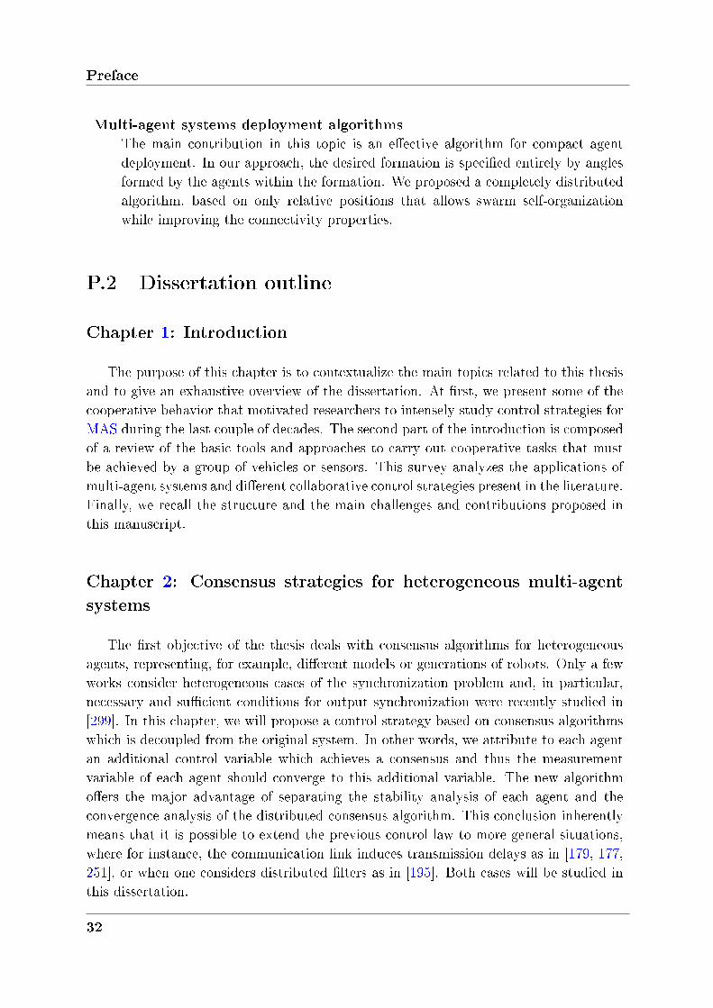
Multi-agent systems deployment algorithms
The main contribution in this topic is an eective algorithm for compact agentdeployment. In our approach, the desired formation is specied entirely by anglesformed by the agents within the formation. We proposed a completely distributedalgorithm, based on only relative positions that allows swarm self-organizationwhile improving the connectivity properties.
P.2 Dissertation outline
Chapter 1: Introduction
The purpose of this chapter is to contextualize the main topics related to this thesisand to give an exhaustive overview of the dissertation. At rst, we present some of thecooperative behavior that motivated researchers to intensely study control strategies forMAS during the last couple of decades. The second part of the introduction is composedof a review of the basic tools and approaches to carry out cooperative tasks that mustbe achieved by a group of vehicles or sensors. This survey analyzes the applications ofmulti-agent systems and dierent collaborative control strategies present in the literature.Finally, we recall the structure and the main challenges and contributions proposed inthis manuscript.
Chapter 2: Consensus strategies for heterogeneous multi-agent
systems
The rst objective of the thesis deals with consensus algorithms for heterogeneousagents, representing, for example, dierent models or generations of robots. Only a fewworks consider heterogeneous cases of the synchronization problem and, in particular,necessary and sucient conditions for output synchronization were recently studied in[299]. In this chapter, we will propose a control strategy based on consensus algorithmswhich is decoupled from the original system. In other words, we attribute to each agentan additional control variable which achieves a consensus and thus the measurementvariable of each agent should converge to this additional variable. The new algorithmoers the major advantage of separating the stability analysis of each agent and theconvergence analysis of the distributed consensus algorithm. This conclusion inherentlymeans that it is possible to extend the previous control law to more general situations,where for instance, the communication link induces transmission delays as in [179, 177,251], or when one considers distributed lters as in [195]. Both cases will be studied inthis dissertation.
32
P.2 Dissertation outline
Chapter 3: Improved stability of consensus algorithms
While in the previous chapter we focused on the design of eective consensus algo-rithms, in this chapter we will pay special attention to consensus algorithm's convergencerate. The speed of convergence of a consensus algorithm turns out to be equal to thesecond smallest eigenvalue of L, also called algebraic connectivity. Accelerating the con-vergence of distributed synchronization algorithms have been studied in literature basedon two main approaches: optimizing the topology-respecting weight matrix, summarizingthe updates at each node [304], or incorporating memory into the distributed averagingalgorithm. This approach will be studied throughout this manuscript. Although for mostapplications delays lead to a reduction of performances or can even lead to instability,there exist some cases where the introduction of a delay in the control loop can help tostabilize a system. This has been studied in [110] and [252]. For this second approach,adding a state sampled component to the control law can be seen as an articial wayto manipulate L's eigenvalues, by getting them further into the left part of the complexplan. This inherently means that the speed of convergence will change, and our objectiveis to maximize this value.
Chapter 4: Distributed control strategies for multi-agent systems
compact formations
This third chapter addresses the design and analysis of an algorithm for compactagent deployment. In our approach, the desired formation is specied entirely by anglesformed by the agents within the formation. We propose a completely leaderless anddistributed algorithm that allows swarm self-organization. The rst contribution corre-sponds to an extension of [76] for swarm dispersion, by adding a connectivity maintenanceforce. Each agent is equipped with potential functions that will, simultaneously, isolateit from any other agent and impose connectivity-maintenance, using only information ofthose located within each agent's sensing zone (a circular area around each agent andcommon for all nodes). We can nd in the literature several applications of this typeof algorithm including coverage control and optimal placement of a multi-robot teamin small areas [63, 90]. On the other hand, and even though bearing-based algorithmswere specically applied to a triangular formation in [9], where the desired formationis specied entirely by the internal triangle angles, the approach that is going to bepresented in the sequel consists of a completely distributed algorithm that allows largescale swarm self-organization. In fact, the second contribution consists of direct anglecontrol using only relative positions. To the best of the author's knowledge, the designof a control law capable of establishing a specic formation acting on inter-agent angleshas not been addressed so far. Two independent problems will be treated separately:dispersion and compactness. An individual stability analysis for these two strategies
33
Preface
will be provided, but we will also propose a sequential control strategy gathering thetwo components. Theoretical arguments and calculations supporting the argument thatsuch system corresponds to a hybrid system will also be discussed. We assume that noglobal positioning system such as the Global Position System (GPS) is available andthat agents interact locally.
Chapter 5: Conclusion and future works
In the last chapter of the thesis, we make a general conclusion, which summarizesthe dissertation contributions and describes ongoing and possible future extensions. Ap-pendix A reviews the fundamentals of sampled systems needed for a complete under-standing of the technical developments of this thesis.
P.3 List of publications
Journal articles under preparation
∙ Gabriel Rodrigues de Campos, Alexandre Seuret, Improved stability of con-
sensus algorithms for MAS using appropriated sampling .∙ Gabriel Rodrigues de Campos, Dimos Dimarogonas, Alexandre Seuret, Karl HenrikJohansson Distributed control strategy for MAS compact Formations .
Proceedings of peer-reviewed international conferences
∙ Gabriel Rodrigues de Campos, Alexandre Seuret, Improved consensus algo-
rithms using memory effects . In Proceedings of the 50𝑡ℎ IEEE Conferenceon Decision and Control and European Control Conference (IEEE CDC/ECC'11),Orlando, USA, 2011
∙ Gabriel Rodrigues de Campos, Alexandre Seuret, Continuous-time double in-
tegrator consensus algorithms improved by an appropriate sampling . InProceedings of the 2𝑛𝑑 IFAC Workshop on Distributed Estimation and Control inNetworked Systems (NecSys'10), Annecy, France, 2010
∙ Gabriel Rodrigues de Campos, Lara Briñón-Arranz, Alexandre Seuret, and SiviuNiculescu, On the consensus of heterogeneous multi-agent systems: a de-
coupling approach . In Proceedings of the 3𝑟𝑑 IFAC Workshop on DistributedEstimation and Control in Networked Systems (NecSys'12), Santa Barbara, USA,2012
34
P.3 List of publications
Peer-reviewed national conference papers
∙ Gabriel Rodrigues de Campos, Alexandre Seuret, Algorithmes de consensus
pour des systèmes double intégrateur continus améliorés par un échan-
tillonnage approprié . In 4𝑚𝑒𝑠 Journées Doctorales /Journées Nationales MACS,Marseille, France, 2011
Extended abstracts
∙ Gabriel Rodrigues de Campos, Iman Shames and Adrian Bishop, Distributedlabeling in autonomous agent populations . In 20𝑡ℎ International Symposiumon Mathematical Theory of Networks and Systems, 2012.
Technical reports
∙ Alexandre Seuret, Daniel Simon, Emilie Roche, Lara Briñón-Arranz and GabrielRodrigues de Campos, Multi-agent systems architecture . D01.03 Buildingblocks and architectures, Deliverable FeedNetBack project, 26 February 2010
35

Preface
36
Chapter 1
Introduction
Contents
1.1 Nature, source of inspiration . . . . . . . . . . . . . . . . . . . 38
1.2 Engineering perception: towards multi-robot systems . . . . 41
1.2.1 What is an agent? . . . . . . . . . . . . . . . . . . . . . . . . . 42
1.2.2 Networking . . . . . . . . . . . . . . . . . . . . . . . . . . . . . 45
1.2.3 Graph theory: concepts and tools . . . . . . . . . . . . . . . . . 47
1.2.4 Distributed control strategies . . . . . . . . . . . . . . . . . . . 51
1.2.5 Multi-robot systems, their applications and challenges . . . . . 59
1.3 General objectives . . . . . . . . . . . . . . . . . . . . . . . . . 62
1.4 Contributions of the thesis . . . . . . . . . . . . . . . . . . . . 65
1.4.1 Chapter 2: MAS rendezvous . . . . . . . . . . . . . . . . . . . . 65
1.4.2 Chapter 3: MAS deployment . . . . . . . . . . . . . . . . . . . 66
Chapter 1. Introduction
1.1 Nature, source of inspiration
Many infrastructures and service systems nowadays can naturally be described as net-works of a huge number of simple interacting units. Examples come from a large rangeof domains and include biological systems (genetic regulation, ecosystems), economicnetworks (production and distribution networks, nancial networks), social networks(Facebook, Twitter or scientic networks) and, of course, technological networks (inter-net, sensor networks, robotics,...). For example, internet service relays on thousands ofrouters transmitting information all over the world [264], in power networks hundredsof power generators have to synchronize for correct performances [203], and inter-modaltransportation systems consist of many trains, cars or airplanes [116]. All these cases askfor distributed decision making, where the process succeeds if all individuals eventuallyagree on some quantity of interest.
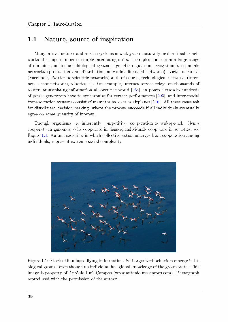
Though organisms are inherently competitive, cooperation is widespread. Genescooperate in genomes; cells cooperate in tissues; individuals cooperate in societies, seeFigure 1.1. Animal societies, in which collective action emerges from cooperation amongindividuals, represent extreme social complexity.
Figure 1.1: Flock of amingos ying in formation. Self-organized behaviors emerge in bi-ological groups, even though no individual has global knowledge of the group state. Thisimage is property of António Luís Campos (www.antonioluiscampos.com). Photographreproduced with the permission of the author.
38
1.1 Nature, source of inspiration
Such societies are not only common in insects, mammals, and birds, but exist evenin simple species like amoebas [268]. During the evolution process that has been takingplace for the last thousands of years, individuals wondering whether to join or not a groupnecessarily weighed the cost-benet ratio of living solitarily versus with others. Whenthe benets of living together outweigh the costs of living alone, animals will tend toform groups. Group-living typically provides benets to individual group members thatmay include receiving assistance to deal with pathogens, easier mating opportunities,better conservation of heat, and reduced energetic costs of movements. However, livingin groups may also confer costs to members such as increased predator attack rate,increased parasite burdens, misdirected parental care, greater reproductive competitionor even increased competition for food. Furthermore, individuals may form short-term,unstable groups, e.g., herds of wildebeest, colonies of gulls, or form long-term, stablesocial groups where interactions among members often appears to be altruistic. Forexample, when a meerkat or a squirrel sounds an alarm call to warn other group membersof a nearby predator, it draws the predator's attention and increases the group's survivalodds [55].
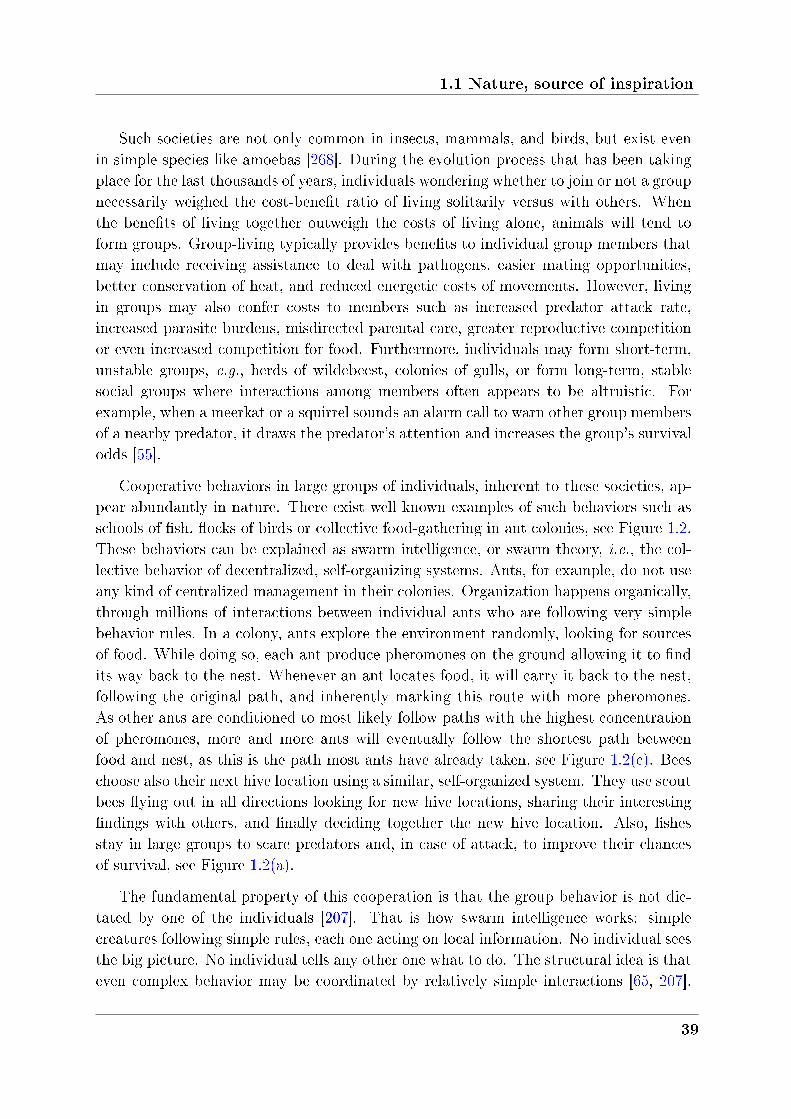
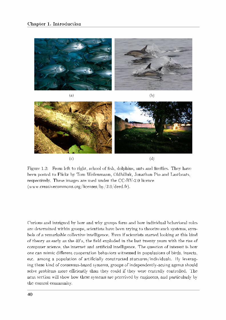
Cooperative behaviors in large groups of individuals, inherent to these societies, ap-pear abundantly in nature. There exist well known examples of such behaviors such asschools of sh, ocks of birds or collective food-gathering in ant colonies, see Figure 1.2.These behaviors can be explained as swarm intelligence, or swarm theory, i.e., the col-lective behavior of decentralized, self-organizing systems. Ants, for example, do not useany kind of centralized management in their colonies. Organization happens organically,through millions of interactions between individual ants who are following very simplebehavior rules. In a colony, ants explore the environment randomly, looking for sourcesof food. While doing so, each ant produce pheromones on the ground allowing it to ndits way back to the nest. Whenever an ant locates food, it will carry it back to the nest,following the original path, and inherently marking this route with more pheromones.As other ants are conditioned to most likely follow paths with the highest concentrationof pheromones, more and more ants will eventually follow the shortest path betweenfood and nest, as this is the path most ants have already taken, see Figure 1.2(c). Beeschoose also their next hive location using a similar, self-organized system. They use scoutbees ying out in all directions looking for new hive locations, sharing their interestingndings with others, and nally deciding together the new hive location. Also, shesstay in large groups to scare predators and, in case of attack, to improve their chancesof survival, see Figure 1.2(a).
The fundamental property of this cooperation is that the group behavior is not dic-tated by one of the individuals [207]. That is how swarm intelligence works: simplecreatures following simple rules, each one acting on local information. No individual seesthe big picture. No individual tells any other one what to do. The structural idea is thateven complex behavior may be coordinated by relatively simple interactions [65, 207].
39
Chapter 1. Introduction
(a) (b)
(c) (d)
Figure 1.2: From left to right, school of sh, dolphins, ants and reies. They havebeen posted to Flickr by Tom Weilenmann, Oldbilluk, Jonathan Pio and Lastbeats,respectively. These images are used under the CC-BY-2.0 licence(www.creativecommons.org/licenses/by/2.0/deed.fr).
Curious and intrigued by how and why groups form and how individual behavioral rolesare determined within groups, scientists have been trying to theorize such systems, sym-bols of a remarkable collective intelligence. Even if scientists started looking at this kindof theory as early as the 40′𝑠, the eld exploded in the last twenty years with the rise ofcomputer science, the internet and articial intelligence. The question of interest is howone can mimic dierent cooperation behaviors witnessed in populations of birds, insects,etc. among a population of articially constructed stuctures/individuals. By leverag-ing these kind of consensus-based systems, groups of independently-acting agents shouldsolve problems more eciently than they could if they were centrally controlled. Thenext section will show how these systems are perceived by engineers, and particularly bythe control community.
40
1.2 Engineering perception: towards multi-robot systems
1.2 Engineering perception: towards multi-robot sys-
tems
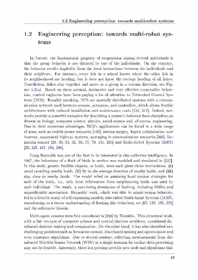
In Nature, the fundamental property of cooperation among several individuals isthat the group behavior is not dictated by one of the individuals. On the contrary,the behavior results implicitly from the local interactions between the individuals andtheir neighbors. For instance, every sh in a school knows where the other sh inits neighborhood are heading, but it does not know the average heading of all shes.Nonetheless, shes stay together and move as a group in a certain direction, see Fig-ure 1.2(a). Based on these natural, instinctive and very eective cooperative behav-iors, control engineers have been paying a lot of attention to Networked Control Sys-tems (NCS). Roughly speaking, NCS are spatially distributed systems with a commu-nication network used between sensors, actuators, and controllers, which allows exiblearchitectures with reduced installation and maintenance costs [120, 311]. Indeed, net-works provide a powerful metaphor for describing a system's behavior from disciplines asdiverse as biology, computer science, physics, social science and, of course, engineering.Due to their numerous advantages, NCS's applications can be found in a wide rangeof areas such as mobile sensor networks [186], remote surgery, haptic collaboration overInternet, automated highway systems, averaging in communication networks [304], for-mation control [29, 30, 31, 32, 35, 75, 79, 131, 283] and Multi-Robot Systems (MRS)[29, 125, 167, 194, 286].
Craig Reynolds was one of the rst to be interested in this collective intelligence. In1987, the behaviour of a ock of birds in motion was modeled and simulated in [227].In this work, generic birdlike objects, or boids, were each given three instructions: (i)avoid crowding nearby boids, (ii) y in the average direction of nearby boids, and (iii)stay close to nearby boids. The model relied on assuming local motion strategies foreach of the boids, i.e., only local information from neighbouring boids was used byeach individual. The result: a convincing simulation of ocking, including lifelike andunpredictable movements. Reynolds' work, which was able to mimic swarm behavior,led to a frenetic study of self-organizing models, also called Multi-Agent Systems (MAS),contributing to a better understanding of ocking like behaviors, see [65, 120, 191, 220]and the references therein.
Multi-agent systems were rst considered in [288] by Tsitsiklis. This structural work,with a fair mixture of computer science and control/decision problems, considered dis-tributed decision making and computation. On the other hand, it has also identied newchallenging problems such as formation control, distributed sensing and optimization andeven consensus algorithms. Due to several reasons, collecting measurements from dis-tributed Wireless Sensor Network (WSN) at a single location for on-line data processingmay not be feasible. Inherently, there is a growing need for new tools and algorithms that
41
Chapter 1. Introduction
provide high performance in terms of control and estimation with constrained communi-cation. Such algorithms should be robust to node failures and packet losses, reduce thecommunication load among all sensor nodes or be suitable for distributed control appli-cations. Even though not discussed in this dissertation, several important contributionson MAS are distributed optimal control [214, 234], distributed estimation [1, 2, 194],distributed Kalman ltering [180, 190, 261], distributed computation [20, 27].
Self-organized swarming behaviors in biological groups with distributed agent-to-agent interactions [58, 65, 188] have become the scientic motivation for studying amongall problems related with multi-agent system, coordination mechanisms of articial mo-bile robots, see [225] for a overview of recent research. In particular, a lot of attentionhas been given to motion coordination, a remarkable phenomenon in biological systems.In nature, of course, animals travel in impressive large numbers. For these animals,coordinating their movements with one another can be a matter of life or death. Severalexamples can be identied, from basic molecules interactions to complex high order ani-mal coordinated groups: we can mention how ocks of birds and schools of sh can travelin formation and act as one unit in order to scare predators and, in the case of attack,to improve their chances of survival; how reies synchronize their ashing cycles; howanimals migrate, showing complex collective behaviors such as obstacle avoiding, leaderelection, and formation keeping; or even environment partitioning into nonoverlappingzones by individual animals. It is then clear that a deep understanding of such behavioris extremely useful tool for groups of vehicles, mobile sensors, and embedded roboticsystems.
A common base to all this works relays on cooperative algorithms. The naturalcooperative strategies observed in Nature (see Figure 1.2) might have dierent form,structure, or scale, but they do aim for the same thing: optimize a task by using all thetools available, i.e., all the individuals. The criteria for the optimization might also bedierent from one example to another.
In order to explain the benets of MAS to control engineering, some basic conceptsand denitions need to be detailed. The rst question that one might ask is "What is anAgent?". Within the scope of this thesis, an answer will be provided in the next section.
1.2.1 What is an agent?
The computer science community has produced various denitions for an agent, asfor example in [115, 235, 300]. A comparison between these denitions and their relativemerits and weaknesses, from a computer science point of view, can be found in [265].Even though dierent, all the denitions referenced above share a basic set of concepts:the notion of an agent, its environment and autonomy. If we consider the environmentas all external elements to the agent, that can be physical (e.g. the control system)
42

1.2 Engineering perception: towards multi-robot systems
or computing related (e.g. data sources, computing resources, and other agents), then,under Wooldridge's denition [300], we call it an agent if it can act autonomously inresponse to environmental changes. This denition is suciently close to those commonlyused by the control community. In the scope of this dissertation, we consider an agentunder the broad denition provided in [92]. An agent is a physical or virtual entityhaving several important characteristics:
∙ Reactivity capabilities: An agent is able to act and has a behaviour to satisfyits goals.
∙ Autonomy: An agent is at least partially autonomous.∙ Perception: It is able to perceive its environment.∙ Local views: No agent has a full global view of the system, or the system is toocomplex for an agent to make practical use of such knowledge.
∙ Communication capabilities: An agent is able to communicate with otheragents.
Note that all these properties are closely related to those of many animals in Nature,where each one of them autonomously perceive and reacts to its environnement whilelocally communicating with those around it. Furthermore, note also that Wooldridgealso dened an intelligent agent by extending the denition of autonomy to exibleautonomy, see [300] for more details.
But to what exactly corresponds an agent? How do we mathematically representindividuals? From engineers' point of view, an agent is nothing more than a dynamicalequation. In fact, this equation states the relation between the input, or in other wordsthe instructions, and the individual's behaviour, i.e., the system's output. In the liter-ature, dierent models to represent the dynamics of an agent have been used. Considera multi-agent system formed by 𝑖 = 1, . . . , 𝑁 agents. The state of agent 𝑖 is representedby 𝑞𝑖 ∈ R𝑚 where 𝑚 is the dimension of the state, and the control input of the system isdenoted by 𝑢𝑖. Two major type of dynamics are available: linear and non linear models.
A) Linear models
i) General linear models
A general linear kinematic model for the agents is described by the followingequations:
𝑞𝑖 =𝐴𝑞𝑖 +𝐵𝑢𝑖, (1.2.1a)
𝑦𝑖 =𝐶𝑞𝑖, (1.2.1b)
where 𝐴,𝐵,𝐶 are matrices of appropriated dimensions. This model is used inliterature mainly dealt with formation control design such as in [88, 89, 105,109, 154].
43
Chapter 1. Introduction
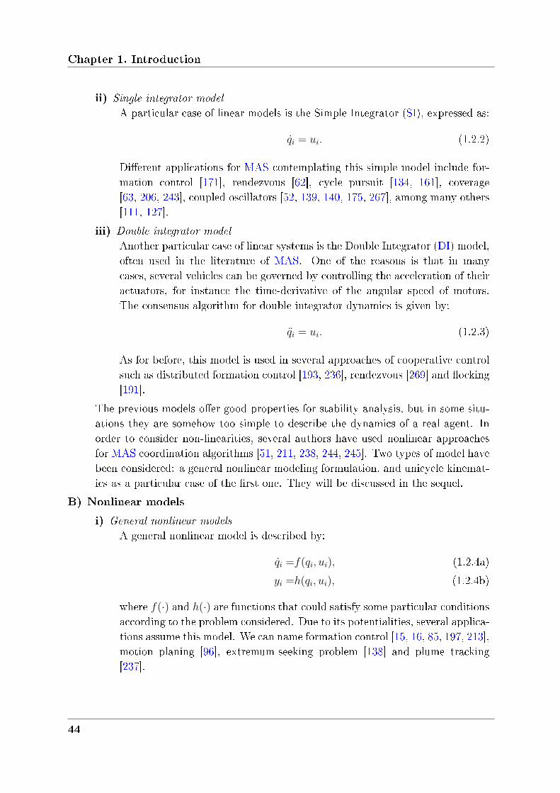
ii) Single integrator model
A particular case of linear models is the Simple Integrator (SI), expressed as:
𝑞𝑖 = 𝑢𝑖. (1.2.2)
Dierent applications for MAS contemplating this simple model include for-mation control [171], rendezvous [62], cycle pursuit [134, 161], coverage[63, 206, 243], coupled oscillators [52, 139, 140, 175, 267], among many others[111, 127].
iii) Double integrator model
Another particular case of linear systems is the Double Integrator (DI) model,often used in the literature of MAS. One of the reasons is that in manycases, several vehicles can be governed by controlling the acceleration of theiractuators, for instance the time-derivative of the angular speed of motors.The consensus algorithm for double integrator dynamics is given by:
𝑞𝑖 = 𝑢𝑖. (1.2.3)
As for before, this model is used in several approaches of cooperative controlsuch as distributed formation control [193, 236], rendezvous [269] and ocking[191].
The previous models oer good properties for stability analysis, but in some situ-ations they are somehow too simple to describe the dynamics of a real agent. Inorder to consider non-linearities, several authors have used nonlinear approachesfor MAS coordination algorithms [51, 211, 238, 244, 245]. Two types of model havebeen considered: a general nonlinear modeling formulation, and unicycle kinemat-ics as a particular case of the rst one. They will be discussed in the sequel.
B) Nonlinear models
i) General nonlinear models
A general nonlinear model is described by:
𝑞𝑖 =𝑓(𝑞𝑖, 𝑢𝑖), (1.2.4a)
𝑦𝑖 =ℎ(𝑞𝑖, 𝑢𝑖), (1.2.4b)
where 𝑓(·) and ℎ(·) are functions that could satisfy some particular conditionsaccording to the problem considered. Due to its potentialities, several applica-tions assume this model. We can name formation control [15, 16, 85, 197, 213],motion planing [96], extremum-seeking problem [138] and plume tracking[237].
44
1.2 Engineering perception: towards multi-robot systems
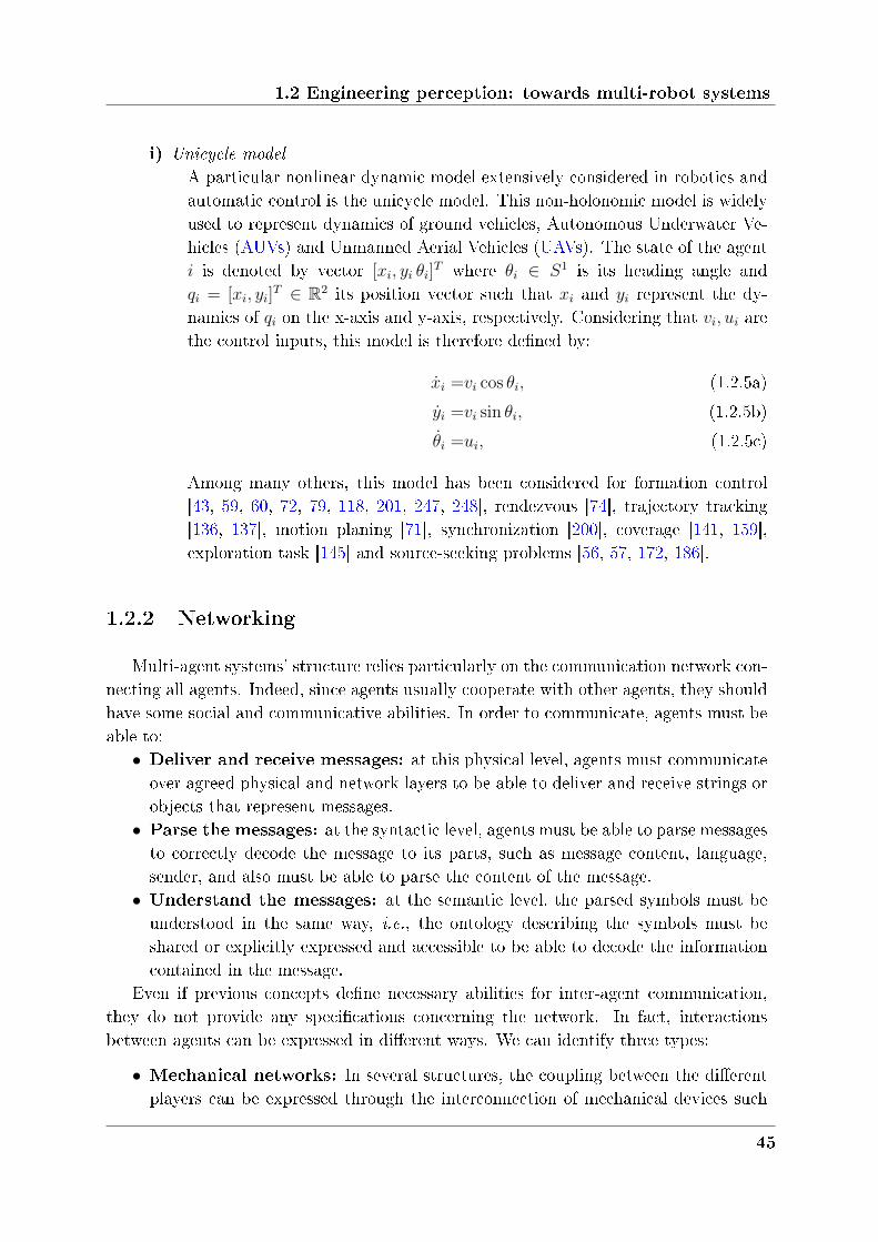
i) Unicycle model
A particular nonlinear dynamic model extensively considered in robotics andautomatic control is the unicycle model. This non-holonomic model is widelyused to represent dynamics of ground vehicles, Autonomous Underwater Ve-hicles (AUVs) and Unmanned Aerial Vehicles (UAVs). The state of the agent𝑖 is denoted by vector [𝑥𝑖, 𝑦𝑖 𝜃𝑖]
𝑇 where 𝜃𝑖 ∈ 𝑆1 is its heading angle and𝑞𝑖 = [𝑥𝑖, 𝑦𝑖]
𝑇 ∈ R2 its position vector such that 𝑥𝑖 and 𝑦𝑖 represent the dy-namics of 𝑞𝑖 on the x-axis and y-axis, respectively. Considering that 𝑣𝑖, 𝑢𝑖 arethe control inputs, this model is therefore dened by:
𝑖 =𝑣𝑖 cos 𝜃𝑖, (1.2.5a)
𝑖 =𝑣𝑖 sin 𝜃𝑖, (1.2.5b)
𝜃𝑖 =𝑢𝑖, (1.2.5c)
Among many others, this model has been considered for formation control[43, 59, 60, 72, 79, 118, 201, 247, 248], rendezvous [74], trajectory tracking[136, 137], motion planing [71], synchronization [200], coverage [141, 159],exploration task [145] and source-seeking problems [56, 57, 172, 186].
1.2.2 Networking
Multi-agent systems' structure relies particularly on the communication network con-necting all agents. Indeed, since agents usually cooperate with other agents, they shouldhave some social and communicative abilities. In order to communicate, agents must beable to:
∙ Deliver and receive messages: at this physical level, agents must communicateover agreed physical and network layers to be able to deliver and receive strings orobjects that represent messages.
∙ Parse the messages: at the syntactic level, agents must be able to parse messagesto correctly decode the message to its parts, such as message content, language,sender, and also must be able to parse the content of the message.
∙ Understand the messages: at the semantic level, the parsed symbols must beunderstood in the same way, i.e., the ontology describing the symbols must beshared or explicitly expressed and accessible to be able to decode the informationcontained in the message.
Even if previous concepts dene necessary abilities for inter-agent communication,they do not provide any specications concerning the network. In fact, interactionsbetween agents can be expressed in dierent ways. We can identify three types:
∙ Mechanical networks: In several structures, the coupling between the dierentplayers can be expressed through the interconnection of mechanical devices such
45
Chapter 1. Introduction
as rigid bodies, springs, dampers or transmissions, satisfying both physical andmechanical properties. Moreover, the same concepts are also used in biology to de-ne interactions between proteins or in neuro-science to express neurones' couplinglaws.
∙ Wired networks: This type of network relies on a system of cables. There aremany areas of application for wired networks. Electric, telephone, cable televisionor computational networks are some examples. In particular, the Ethernet is awidely used technology to establish a Local Area Network (LAN). More precisely,these structures are dened by a group of computers and associated devices thatshare a common communication line within a very small geographical area. Fur-thermore, it is also possible that several devices have to share the resources of asingle processor or server.
∙ Wireless networks: Since having a wired connection is impossible in spatiallydistributed plants or in cars and airplanes, there is a lot of interest in wirelessnetworks. The word wireless is dened in the dictionary as "having no wires". Innetworking terminology, wireless is the term used to describe any network wherethere is no physical wired connection between sender and receiver, but rather acommunication network based on radio wave transmissions. A common applicationin every day life is the portable oce. People on the road want to use their portableelectronic equipment to send and receive telephone calls, faxes, and electronic mail,read remote les, login on remote machines and do this from anywhere on land, sea,or air. Wireless networks are of great value to eets of trucks, taxis, buses, trainsor planes. Another use is for rescue workers at disaster sites where the telephonesystem has been destroyed.
The introduction of the communication network in multi-agent systems oers someadvantages, such as low cost, high reliability, less wiring, easy maintenance, but alsovarious communication constraints including quantization eects [38, 44, 132], presenceof noise [157, 318], delayed communication [42, 153, 157, 194, 274, 275, 284, 285, 301,302, 310, 318], packet losses [86, 113, 209, 276, 306] and so on. More precisely, forrst order multi-agent systems, [194] gives an initial study on the consensus problem forcontinuous-time systems in the frequency domain and provides a necessary and sucientcondition on the upper bound of time-delays under the assumption that all the delays areequal and time-invariant. For multi-agent systems with dynamically changing topologiesand time-varying communication delays, [42, 301] prove that multi-agent systems canreach consensus under some connectivity condition, irrespective of time delays. Wheninput delay also exists, a sucient condition is provided in [284]. In [114, 209, 276],rst-order consensus problem is formulated over networks with random packet losses,where it is shown that almost sure consensus is achieved if the expected interactiontopology has spanning trees. Considering second-order consensus protocols, [153, 285]investigate the eect of constant input delays on the protocol's convergence properties
46
1.2 Engineering perception: towards multi-robot systems
and provides delay-dependent consensus conditions. Moreover, [318] investigates theconsensus of second-order networked multi-agent systems with noise, packet losses andrandom communication delays. A queuing mechanism is introduced and the inherentpacket loss process is assumed to obey the Bernoulli distribution.
In other elds, multi-agent systems are often addressed by computer science [92, 125,290], distributed computation [20, 27], game theory [28] or social science [68]. In order tomodel multi-agent systems, control engineers use several tools and denitions from graphtheory. The reader should refer to [23, 117, 238] and the references therein for detailedinformation. Next section presents the necessary tools used throughout the technicaldevelopments of this thesis.
1.2.3 Graph theory: concepts and tools
In a simplied way, MAS can be graphically represented by a network of nodesinterconnected via communication links, usually modeled by arrows. In the context ofthis thesis, the existence of an edge necessarily means that the two concerned agents canexchange information. One should note that the graph connecting agents can be eitherdirected or undirected. Therefore, the two following denitions hold.
Definition 1.1. A direct graph or digraph is defined as a couple 𝒢 = (𝑉,𝐸) consisting
of a set of 𝑁 elements called vertices, denoted by 𝑉 = 1, 2, . . . , 𝑁 and a set of ordered
pair of vertices called edges, represented by 𝐸 ⊆ 𝑉 × 𝑉 . The pair (𝑖, 𝑗) denotes an edge
from the element 𝑖 to 𝑗.
Definition 1.2. An undirected graph consists of a set of vertices 𝑉 and a set of edges
𝐸 such that, for all pair of elements 𝑖, 𝑗 ∈ 𝑉 , (𝑖, 𝑗) ∈ 𝐸 and (𝑗, 𝑖) ∈ 𝐸.
As mentioned before, in MAS the group behavior is not dictated by one of the in-dividuals. On the contrary, the behavior results implicitly from the local interactionsbetween the individuals and their neighbors. Even if previously summarized, the follow-ing denition formalizes the neighborhood concept.
Definition 1.3. The neighborhood of a vertex 𝑖 ∈ 𝑉 is the set:
𝒩𝑖 = 𝑗 ∈ 𝑉 |(𝑖, 𝑗) ∈ 𝐸.
Therefore, all the elements 𝑗 ∈ 𝒩𝑖 are called the neighbors of element 𝑖. This meansthat there is an edge from node 𝑖 to each node 𝑗 which belongs to the neighborhood.This inherently leads us to the following denition concerning node degree.
Definition 1.4. The degree of a vertex 𝑖 ∈ 𝑉 is the number of its neighbors, such that
𝑑𝑖 = |𝒩𝑖|.
47
Chapter 1. Introduction
The previous denition allows us to dene, in a matrix form, how many neighborseach agent has through what is called the degree matrix, dened as follows.
Definition 1.5. The degree matrix of a digraph 𝒢 = (𝑉,𝐸) is the 𝑁 × 𝑁 matrix
∆ = (𝑑𝑖𝑗) given for all 𝑖, 𝑗 ∈ 𝑉 by:
𝑑𝑖𝑗 =
𝑑𝑖, if 𝑖 = 𝑗
0 otherwise
Until now, we have modeled and dened all concepts related to MAS except how andfrom who to who information is exchanged. This can be modeled through what is calledadjacency matrix dened as follows.
Definition 1.6. The adjacency matrix of a digraph 𝒢 = (𝑉,𝐸) is the 𝑁 ×𝑁 matrix
𝒜 = (𝑎𝑖𝑗) given for all 𝑖, 𝑗 ∈ 𝑉 by:
𝑎𝑖𝑗 =
1, if (𝑖, 𝑗) ∈ 𝐸,
0 otherwise.
Both adjacency and degree matrices have been previously dened. We are now readyto introduce what is called in literature the Laplacian matrix L. This new matrix,which gathers both information of adjacency and neighborhood for each agent 𝑖, can beexpressed as:
L = ∆ −𝒜,and therefore
𝐿𝑖𝑗 =
⎧⎨⎩𝑑𝑖, if 𝑖 = 𝑗,
−1, if 𝑗 ∈ 𝒩𝑖,
0 otherwise.(1.2.6)
where 𝐿𝑖𝑗 denotes the element on 𝑖𝑡ℎ line and 𝑗𝑡ℎ column of 𝐿, which is a 𝑁 × 𝑁 sizematrix. One should note that ∆ is a diagonal matrix, and by denition, each diagonalelement of the degree matrix is equal to the sum of elements of its corresponding rowin the adjacency matrix (∆)𝑖𝑖 =
∑𝑁𝑗=1 𝑎𝑖𝑗. Moreover, all the eigenvalues of L have
nonnegative real parts, such that:
0 = 𝜆0 ≤ 𝜆1 ≤ . . . ≤ 𝜆𝑁−1,
where 𝜆𝑘(L) represents the 𝑘𝑡ℎ eigenvalue of L. It is worth mentioning that the secondsmallest eigenvalue of graph's Laplacian, called algebraic connectivity, quanties thespeed of convergence of consensus algorithms. The following denition holds.
48
1.2 Engineering perception: towards multi-robot systems
Definition 1.7. The second smallest eigenvalue 𝜆2 of the Laplacian matrix L is referred
to as the algebraic connectivity of the undirected graph 𝒢.
Laplacians and their spectral properties [106, 168] play a crucial role in convergenceanalysis of consensus and alignment algorithms. In fact, several agreement algorithmscan be formalized using the previously dened Laplacian matrix, and consequently, theirconvergence properties are dependent on the structure and derived properties of L. Oneof the several interesting properties of L states that the vector of ones 1 = (1, . . . , 1)𝑇 ∈R𝑁 is always an eigenvector of the Laplacian matrix with eigenvalue zero, such that,L1 = 0, where 0 = (0, . . . , 0)𝑇 ∈ R𝑁 represents the vector of zeros.
Another concept that drastically aects convergence properties of consensus algo-rithms is graph's connectivity. The notion of connectivity is associated to the idea thatthe information transmitted by one node in the graph can be received for the rest of thenodes of the communication graph.
Consider a digraph 𝒢 = (𝑉,𝐸) whose vertices are denoted by 𝑉 = 𝑖1, 𝑖2, . . . , 𝑖𝑁. Avertex of a digraph is globally reachable if it can be reached from any other vertex bytraversing a direct path, which is dened as follows.
Definition 1.8. A direct path in a digraph 𝒢 = (𝑉,𝐸) is an ordered sequence of vertices
(𝑖1, 𝑖2)(𝑖2, 𝑖3) . . . (𝑖𝑚−1, 𝑖𝑚) such that any ordered pair of vertices appearing consecutively
in the sequence is an edge of the digraph, i.e., (𝑖𝑝−1, 𝑖𝑝) ∈ 𝐸 for all 𝑝 = 1, . . . ,𝑚, where
𝑚 ≤ 𝑁 .
In literature, there exist a huge number of contributions that rely on the propertiesof the Laplacian matrix. However, most solutions proposed in these works are graphconstrained. In other words, strong assumption are made on the communication graph.In order to discuss, further in this thesis, assumption conservativeness, the followingdenitions hold.
Definition 1.9. A digraph 𝒢 = (𝑉,𝐸) is strongly connected if every vertex is globally
reachable, such that, for all 𝑘 ∈ 𝑉 there is a direct path starting from each other vertex
𝑗 ∈ 𝑉, 𝑗 = 𝑘 which finishes in 𝑘.
Definition 1.10. A digraph is balanced if each vertex 𝑘 ∈ 𝑉 has the same number of
incoming and outgoing edges.
Requiring a strongly connected and balanced graph is, in fact, a very conservativeassumption. However, and under xed interaction topologies, it has been shown in [220]that agreement algorithms such as consensus asymptotically converge if and only if thedirected interaction topology has a directed spanning tree. Therefore, the following threedenitions are needed.
49
Chapter 1. Introduction
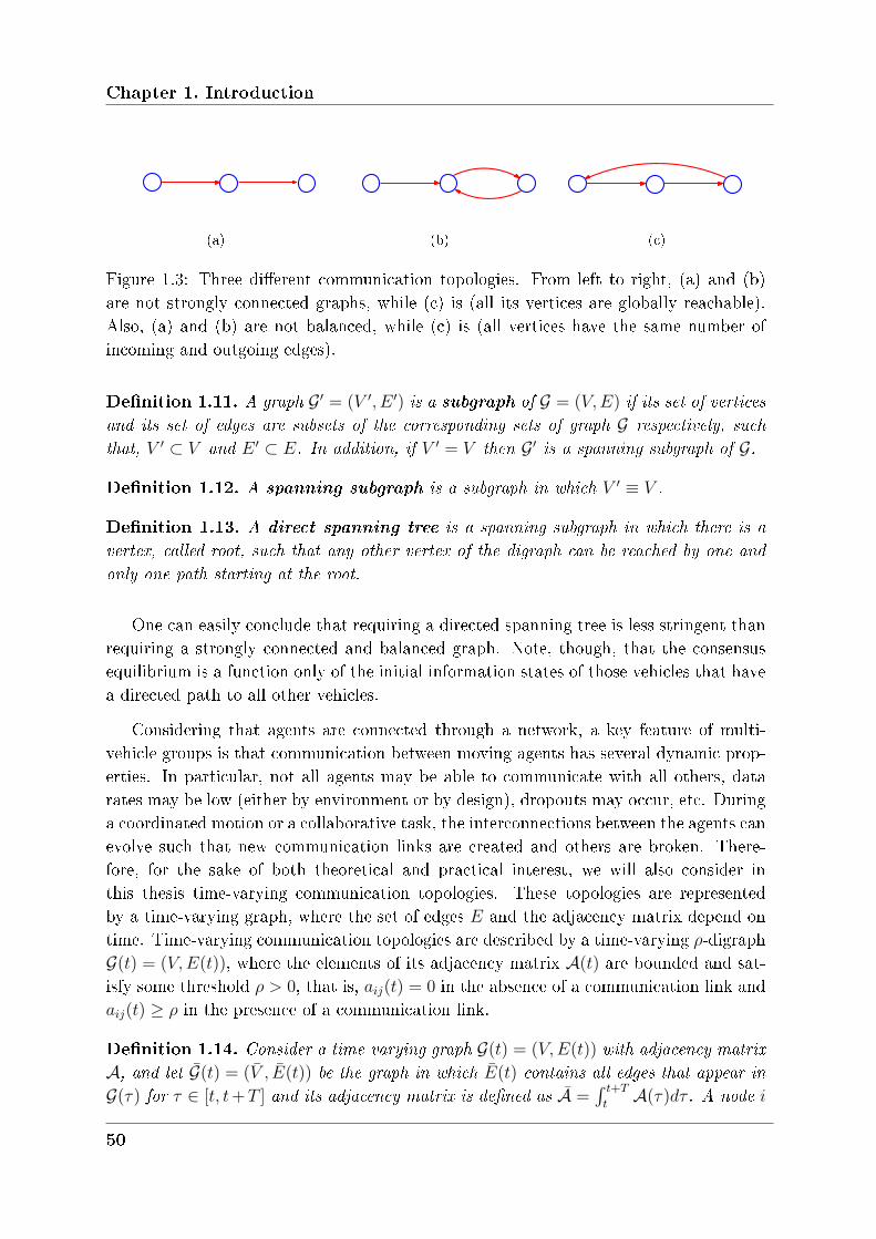
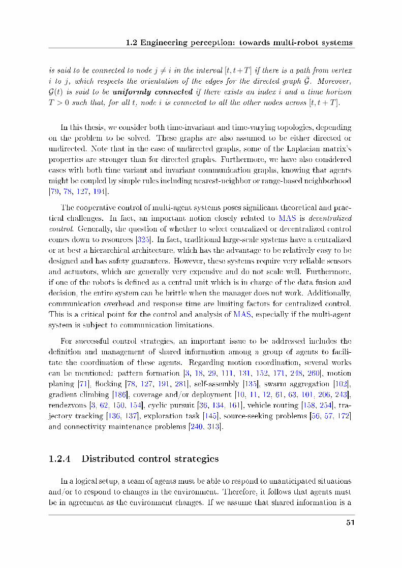
(a) (b) (c)
Figure 1.3: Three dierent communication topologies. From left to right, (a) and (b)are not strongly connected graphs, while (c) is (all its vertices are globally reachable).Also, (a) and (b) are not balanced, while (c) is (all vertices have the same number ofincoming and outgoing edges).
Definition 1.11. A graph 𝒢 ′ = (𝑉 ′, 𝐸 ′) is a subgraph of 𝒢 = (𝑉,𝐸) if its set of vertices
and its set of edges are subsets of the corresponding sets of graph 𝒢 respectively, such
that, 𝑉 ′ ⊂ 𝑉 and 𝐸 ′ ⊂ 𝐸. In addition, if 𝑉 ′ = 𝑉 then 𝒢 ′ is a spanning subgraph of 𝒢.
Definition 1.12. A spanning subgraph is a subgraph in which 𝑉 ′ ≡ 𝑉 .
Definition 1.13. A direct spanning tree is a spanning subgraph in which there is a
vertex, called root, such that any other vertex of the digraph can be reached by one and
only one path starting at the root.
One can easily conclude that requiring a directed spanning tree is less stringent thanrequiring a strongly connected and balanced graph. Note, though, that the consensusequilibrium is a function only of the initial information states of those vehicles that havea directed path to all other vehicles.
Considering that agents are connected through a network, a key feature of multi-vehicle groups is that communication between moving agents has several dynamic prop-erties. In particular, not all agents may be able to communicate with all others, datarates may be low (either by environment or by design), dropouts may occur, etc. Duringa coordinated motion or a collaborative task, the interconnections between the agents canevolve such that new communication links are created and others are broken. There-fore, for the sake of both theoretical and practical interest, we will also consider inthis thesis time-varying communication topologies. These topologies are representedby a time-varying graph, where the set of edges 𝐸 and the adjacency matrix depend ontime. Time-varying communication topologies are described by a time-varying 𝜌-digraph𝒢(𝑡) = (𝑉,𝐸(𝑡)), where the elements of its adjacency matrix 𝒜(𝑡) are bounded and sat-isfy some threshold 𝜌 > 0, that is, 𝑎𝑖𝑗(𝑡) = 0 in the absence of a communication link and𝑎𝑖𝑗(𝑡) ≥ 𝜌 in the presence of a communication link.
Definition 1.14. Consider a time-varying graph 𝒢(𝑡) = (𝑉,𝐸(𝑡)) with adjacency matrix
𝒜, and let 𝒢(𝑡) = (𝑉 , (𝑡)) be the graph in which (𝑡) contains all edges that appear in
𝒢(𝜏) for 𝜏 ∈ [𝑡, 𝑡+𝑇 ] and its adjacency matrix is defined as 𝒜 =∫ 𝑡+𝑇𝑡
𝒜(𝜏)𝑑𝜏 . A node 𝑖
50
1.2 Engineering perception: towards multi-robot systems
is said to be connected to node 𝑗 = 𝑖 in the interval [𝑡, 𝑡+𝑇 ] if there is a path from vertex
𝑖 to 𝑗, which respects the orientation of the edges for the directed graph 𝒢. Moreover,
𝒢(𝑡) is said to be uniformly connected if there exists an index 𝑖 and a time horizon
𝑇 > 0 such that, for all 𝑡, node 𝑖 is connected to all the other nodes across [𝑡, 𝑡+ 𝑇 ].
In this thesis, we consider both time-invariant and time-varying topologies, dependingon the problem to be solved. These graphs are also assumed to be either directed orundirected. Note that in the case of undirected graphs, some of the Laplacian matrix'sproperties are stronger than for directed graphs. Furthermore, we have also consideredcases with both time variant and invariant communication graphs, knowing that agentsmight be coupled by simple rules including nearest-neighbor or range-based neighborhood[79, 78, 127, 194].
The cooperative control of multi-agent systems poses signicant theoretical and prac-tical challenges. In fact, an important notion closely related to MAS is decentralized
control. Generally, the question of whether to select centralized or decentralized controlcomes down to resources [325]. In fact, traditional large-scale systems have a centralizedor at best a hierarchical architecture, which has the advantage to be relatively easy to bedesigned and has safety guarantees. However, these systems require very reliable sensorsand actuators, which are generally very expensive and do not scale well. Furthermore,if one of the robots is dened as a central unit which is in charge of the data fusion anddecision, the entire system can be brittle when the manager does not work. Additionally,communication overhead and response time are limiting factors for centralized control.This is a critical point for the control and analysis of MAS, especially if the multi-agentsystem is subject to communication limitations.
For successful control strategies, an important issue to be addressed includes thedenition and management of shared information among a group of agents to facili-tate the coordination of these agents. Regarding motion coordination, several workscan be mentioned: pattern formation [3, 18, 29, 111, 131, 152, 171, 248, 260], motionplaning [71], ocking [78, 127, 191, 281], self-assembly [135], swarm aggregation [102],gradient climbing [186], coverage and/or deployment [10, 11, 12, 61, 63, 101, 206, 243],rendezvous [3, 62, 150, 154], cyclic pursuit [36, 134, 161], vehicle routing [158, 254], tra-jectory tracking [136, 137], exploration task [145], source-seeking problems [56, 57, 172]and connectivity maintenance problems [240, 313].
1.2.4 Distributed control strategies
In a logical setup, a team of agents must be able to respond to unanticipated situationsand/or to respond to changes in the environment. Therefore, it follows that agents mustbe in agreement as the environment changes. If we assume that shared information is a
51
Chapter 1. Introduction
necessary condition for coordination, a direct consequence is that cooperation requiresthat the group of agents reach consensus on the coordination data. To converge to acommon value is commonly called a consensus or agreement problem in the literature[87, 127, 129, 282].
Serving as an introduction to the technical achievements of this thesis, the nextsection will provide a precise denition of some of these types of algorithms.
Consensus algorithms
We consider a consensus algorithm (or protocol) as an interaction rule that speciesthe information exchange between an agent and all of its neighbors over the network inorder to reach an agreement regarding a certain quantity of interest that depends on thestate of all agents. For example, consensus is a useful algorithm to reach rendezvous,i.e., all the agents converge to the same location [62, 74, 309, 308]. As a special case ofMAS, consensus problems have a long history in the eld of computer science. In fact,these algorithms have their roots in the analysis of Markov chains and have been deeplystudied within the computer science community for load balancing [181, 289] and withinthe linear algebra community for the asynchronous solution of linear systems [99, 266].However, they have been recently rediscovered by the control and robotics communitiesand applied to cooperative coordination of multi-agent systems. In fact, these distributedagreement problems are directly related to mobile multi-robot applications, since theyrepresent an excellent tool to develop more complex cooperative control laws. The readermight refer to [37, 192, 222, 220] and the references therein for thorough information onthis topic.
In the second chapter of this thesis, we pay special attention to consensus algorithms.Even though there are dierent models to represent the dynamics of multi-agent systemsused in literature, in this thesis we mainly consider linear systems. Moreover, as par-ticular cases of linear systems, we have intensively studied simple and double integratordynamics, whose advantages and drawbacks are briey discussed in the sequel.
Consensus algorithms for linear dynamics
Consider a multi-agent system formed by 𝑖 = 1, . . . , 𝑁 agents. As mentioned before,a general linear model can be described as follows:
𝑞𝑖 =𝐴𝑞𝑖 +𝐵𝑢𝑖,
𝑦𝑖 =𝐶𝑞𝑖,
52
1.2 Engineering perception: towards multi-robot systems
where 𝑞, 𝑦 and 𝐴,𝐵,𝐶 have been dened in (1.2.1). Our objective is to design a dis-tributed control law which ensures that the output vectors of each agent reach an agree-ment. Therefore, the consensus algorithm can be written as:
𝑢𝑖 = −𝐾∑𝑗∈𝒩𝑖
(𝑦𝑖 − 𝑦𝑗), (1.2.8)
where 𝐾 > 0 is a control matrix. Specially applied to formation control, this model wasused in [88, 89, 105, 109, 154, 298, 299].
Consensus algorithms for simple integrator dynamics
Another model considered in this thesis is a special case of linear systems. A SI agentcan be describe as:
𝑞𝑖 = 𝑢𝑖.
As for before, in order to achieve state agreement between all agents, a commonlyused SI consensus algorithm [13, 194, 251] is given by:
𝑢𝑖 =∑𝑗∈𝒩𝑖
𝑎𝑖𝑗 (𝑞𝑗 − 𝑞𝑖).
This algorithm is distributed in the sense that each agent has only access to infor-mation from its neighbors, represented by the adjacency 𝑎𝑖𝑗 weights previously denedin Section 1.2.3. Introducing the vector 𝑥(𝑡) = [𝑥1, .., 𝑥𝑁 ]𝑇 containing the state of allagents, we then derive:
𝑞 = −L𝑞 , (1.2.9)
where L is the Laplacian matrix. This simple model is very popular within MAS analysisand control. The reader can nd it applied to dierent applications: formation control[171], rendezvous [62], cycle pursuit [134, 161], coverage [63, 206, 243] among many others[111, 127].
For the sake of thoroughness of this survey, Kuramoto's oscillators will be briey dis-cussed here. Recently, a lot of research eorts focus on the mathematical analysis systemscomposed of interacting phase oscillators. A commonly used model relies on Kuramotoalgorithms or Kuramoto oscillators, introduced in [139]. The proposed synchronizationalgorithm for coupled oscillators is given as:
𝑢𝑖 = −∑𝑗∈𝒩𝑖
sin (𝑞𝑗 − 𝑞𝑖) . (1.2.10)
53
Chapter 1. Introduction
Based on this initial work, several extensions [52, 140, 175, 183, 267] led to a deepunderstanding of the synchronization problem, easily applicable to synchronize and sta-bilize dierent patterns in a MAS conguration, as for example in [199].
Consensus algorithms for double integrator dynamics
Finally, a third model considered in this thesis represents a dierent specic case oflinear systems. Recalling equation (1.2.3), consider vehicles with DI dynamics given by:
𝑞𝑖 = 𝑢𝑖.
One should note that this model ts the behavior of real robotic agents more nat-urally, since such mechanical systems are controlled in most cases through their accel-eration and not their velocity. Moreover, several robotic systems can be reduced to adouble integrator via a transformation in their control law. But DI algorithms leads toseveral problems [217, 224]. For instance, if the graph is directed, the algorithm is notstable, and on the other hand, if the graph is undirected, this requires the knowledgeof both position and velocity to converge to the same value. A consensus algorithm for(1.2.3) is studied in [216, 305] as:
𝑢𝑖 = −∑𝑗∈𝒩𝑖
𝑎𝑖𝑗[(𝑞𝑗 − 𝑞𝑖) + 𝜍𝑞𝑖], (1.2.11)
where 𝑎𝑖𝑗 is the (𝑖, 𝑗)𝑡ℎ entry of the adjacency matrix and 𝜍 a positive control gainrepresenting the absolute damping. Following the same formalism as before, it follows:
𝑞(𝑡) = −𝜍𝑞 − L𝑞, (1.2.12)
where L represents the Laplacian matrix. Consensus is reached for (1.2.3) if for all𝑞𝑖(0) and 𝑞𝑖(0), 𝑞𝑖(𝑡) → 𝑞𝑗(𝑡) and 𝑞𝑖(𝑡) → 0 as 𝑡 → ∞. This model is used in severalapproaches of cooperative control such as distributed formation control [193, 236, 323],rendezvous [269] and ocking [191]. Note that this model allows the agents to reachan agreement in their velocities. This particular case of consensus problems is calledocking and, by denition, it is not possible to be applied to simple integrator dynamicsof the agents.
On the other hand, a consensus algorithm for (1.2.3) is studied in [218] as given by:
𝑢𝑖 = −∑𝑗∈𝒩𝑖
𝑎𝑖𝑗[(𝑞𝑗 − 𝑞𝑖) + 𝜚(𝑞𝑗 − 𝑞𝑖)], (1.2.13)
54
1.2 Engineering perception: towards multi-robot systems
where 𝜚 is a positive gain representing the relative damping. Following the same formal-ism as before, it follows:
𝑞(𝑡) = −𝜚L𝑞 − L𝑞 . (1.2.14)
Once again, consensus is reached for (1.2.3) if for all 𝑞𝑖(0) and 𝑞𝑖(0), 𝑞𝑖(𝑡) → 𝑞𝑗(𝑡) and𝑞𝑖(𝑡) → 𝑞𝑗(𝑡) as 𝑡 → ∞. Note that both communication topology and coupling gain 𝜚aect consensus-seeking [220].
The previous discussion provided the essentials on consensus algorithms. Never-theless, there exist a huge number of further contributions on consensus algorithmsconsidering time-delays [26, 251], switching topologies [39, 111, 194, 219], consensus l-ters [192, 195], uncertainties [133], nite-time consensus [273], among many other cases[13, 14, 242, 322].
In this thesis we are particulary interested in collaborative behaviors ensuring goodconnectivity properties. Cohesiveness is characterized by a repulsion/attraction functionwhich makes the agents in the network maintain desired relative distances between itsneighbors or achieve collision avoidance [191, 279]. Due to its pertinence to the technicaldevelopments of the third chapter, a brief denition of these types of systems is presentedin the following.
Inverse Agreement Algorithms
In literature, algorithms whose inverse would lead the multi-agent team to agreementare called dispersion algorithms. The goal is to design control laws that force the agentsto converge to suciently large distances between them, i.e., disperse in the workspace,or eventually to keep a certain distance between agents. In order to full this purpose,several authors used articial potential elds [73, 74, 76]. More precisely, each agentis equipped with a repulsive potential with respect to each other agent. Moreover,agents are considered to have limited communication range, a commonly setup widelyconsidered in literature and specially suited to mobile robot applications. For any twoagents (𝑖, 𝑗), dene the vector connecting agent 𝑖 and 𝑗 as:
𝑞𝑖𝑗 = 𝑞𝑗 − 𝑞𝑖,
and the squared distance between two agents as:
𝛽𝑖𝑗 = ‖𝑞𝑗 − 𝑞𝑖‖2, ∀ 𝑖, 𝑗 ∈ 𝒩 .
The goal is for each agent to follow a ow, whose inverse leads the multi-agent team toagreement, just by taking in consideration the relative positions of agents located withineach agent's sensing zone (a circular area of radius 𝑑 around each agent and common for
55
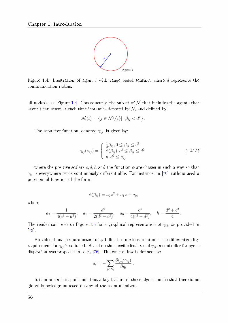
Chapter 1. Introduction
Agent i
d
Figure 1.4: Illustration of agent 𝑖 with range based sensing, where 𝑑 represents thecommunication radius.
all nodes), see Figure 1.4. Consequently, the subset of 𝒩 that includes the agents thatagent 𝑖 can sense at each time instant is denoted by 𝒩𝑖 and dened by:
𝒩𝑖(𝑡) =𝑗 ∈ 𝒩∖𝑖| 𝛽𝑖𝑗 < 𝑑2
.
The repulsive function, denoted 𝛾𝑖𝑗, is given by:
𝛾𝑖𝑗(𝛽𝑖𝑗) =
⎧⎨⎩12𝛽𝑖𝑗, 0 ≤ 𝛽𝑖𝑗 ≤ 𝑐2
𝜑(𝛽𝑖𝑗), 𝑐2 ≤ 𝛽𝑖𝑗 ≤ 𝑑2
ℎ, 𝑑2 ≤ 𝛽𝑖𝑗
(1.2.15)
where the positive scalars 𝑐, 𝑑, ℎ and the function 𝜑 are chosen in such a way so that𝛾𝑖𝑗 is everywhere twice continuously dierentiable. For instance, in [76] authors used apolynomial function of the form:
𝜑(𝛽𝑖𝑗) = 𝑎2𝑥2 + 𝑎1𝑥+ 𝑎0,
where
𝑎2 =1
4(𝑐2 − 𝑑2), 𝑎1 =
𝑑2
2(𝑑2 − 𝑐2), 𝑎0 =
𝑐4
4(𝑐2 − 𝑑2), ℎ =
𝑑2 + 𝑐2
4.
The reader can refer to Figure 1.5 for a graphical representation of 𝛾𝑖𝑗, as provided in[73].
Provided that the parameters of 𝜑 full the previous relations, the dierentiabilityrequirement for 𝛾𝑖𝑗 is satised. Based on the specic features of 𝛾𝑖𝑗, a controller for agentdispersion was proposed in, e.g., [76]. The control law is dened by:
𝑢𝑖 = −∑𝑗∈𝒩𝑖
𝜕(1/𝛾𝑖𝑗)
𝜕𝑞𝑖.
It is important to point out that a key feature of these algorithms is that there is noglobal knowledge imposed on any of the team members.
56
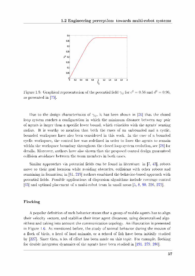
1.2 Engineering perception: towards multi-robot systems
0 0.2 0.4 0.6 0.8 1 1.2 1.4 1.6 1.8 20
0.05
0.1
0.15
0.2
0.25
0.3
0.35
0.4
βij
γ ij
Figure 1.5: Graphical representation of the potential eld 𝛾𝑖𝑗 for 𝑐2 = 0.56 and 𝑑2 = 0.96,as presented in [73].
Due to the design characteristics of 𝛾𝑖𝑗, it has been shown in [76] that the closedloop system reaches a conguration in which the minimum distance between any pairof agents is larger than a specic lower bound, which coincides with the agents' sensingradius. It is worthy to mention that both the cases of an unbounded and a cyclic,bounded workspace have also been considered in this work. In the case of a boundedcyclic workspace, the control law was redened in order to force the agents to remainwithin the workspace boundary throughout the closed loop system evolution, see [76] fordetails. Moreover, authors have also shown that the proposed control design guaranteedcollision avoidance between the team members in both cases.
Similar approaches via potential elds can be found in literature: in [7, 43], robotsmove to their goal location while avoiding obstacles, collisions with other robots andremaining in formation; in [81, 215] authors combined the behavior-based approach withpotential elds. Possible applications of dispersion algorithms include coverage control[63] and optimal placement of a multi-robot team in small areas [5, 8, 90, 226, 272].
Flocking
A popular denition of such behavior states that a group of mobile agents has to aligntheir velocity vectors, and stabilize their inter-agent distances, using decentralized algo-rithms and taking into account the communication topology. An illustration is presentedin Figure 1.6. As mentioned before, the study of animal behavior during the motion ofa ock of birds, a herd of land animals, or a school of sh have been initially studiedby [227]. Since then, a lot of eort has been made on this topic. For example, ockingfor double integrator dynamics of the agents have been studied in [191, 279, 280].
57
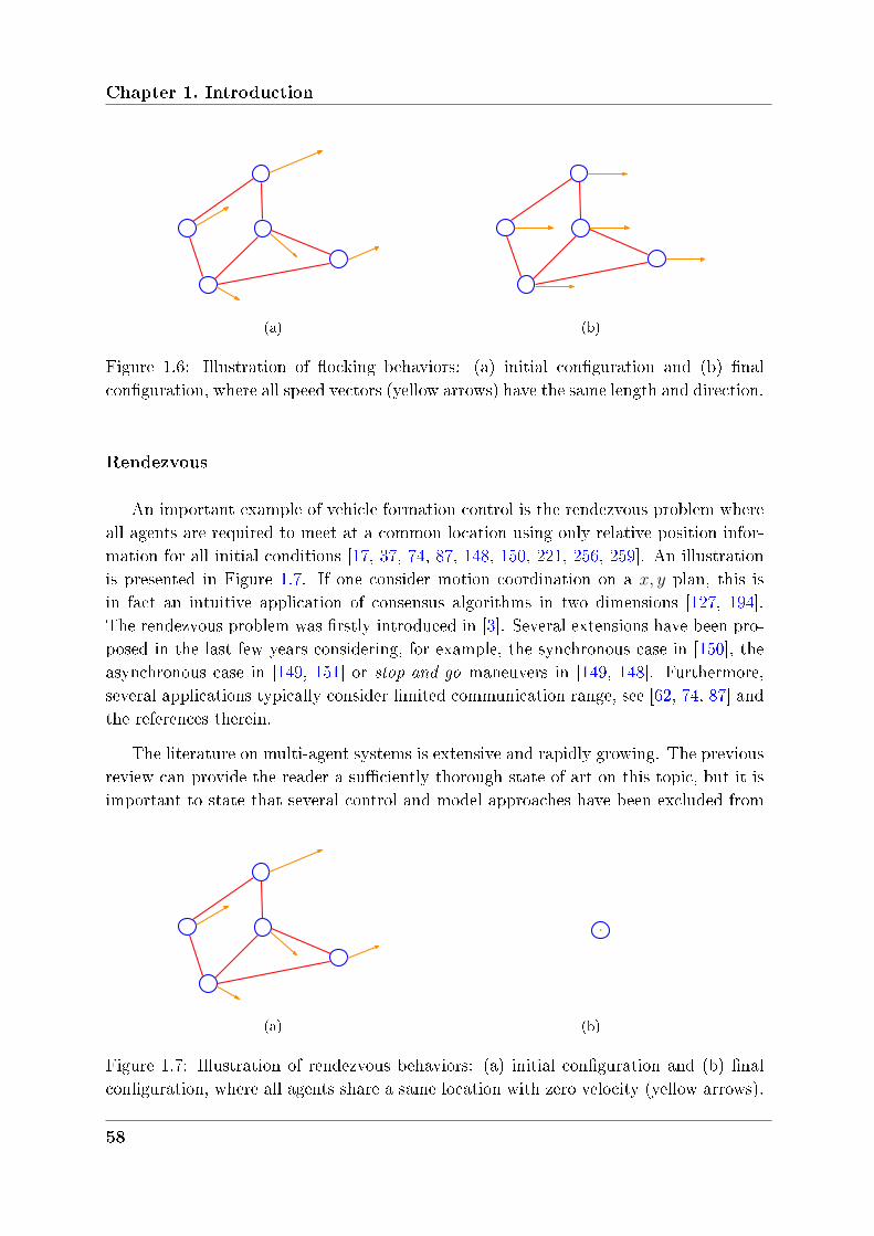
Chapter 1. Introduction
(a) (b)
Figure 1.6: Illustration of ocking behaviors: (a) initial conguration and (b) nalconguration, where all speed vectors (yellow arrows) have the same length and direction.
Rendezvous
An important example of vehicle formation control is the rendezvous problem whereall agents are required to meet at a common location using only relative position infor-mation for all initial conditions [17, 37, 74, 87, 148, 150, 221, 256, 259]. An illustrationis presented in Figure 1.7. If one consider motion coordination on a 𝑥, 𝑦 plan, this isin fact an intuitive application of consensus algorithms in two dimensions [127, 194].The rendezvous problem was rstly introduced in [3]. Several extensions have been pro-posed in the last few years considering, for example, the synchronous case in [150], theasynchronous case in [149, 151] or stop-and-go maneuvers in [149, 148]. Furthermore,several applications typically consider limited communication range, see [62, 74, 87] andthe references therein.
The literature on multi-agent systems is extensive and rapidly growing. The previousreview can provide the reader a suciently thorough state of art on this topic, but it isimportant to state that several control and model approaches have been excluded from
(a) (b)
Figure 1.7: Illustration of rendezvous behaviors: (a) initial conguration and (b) nalconguration, where all agents share a same location with zero velocity (yellow arrows).
58
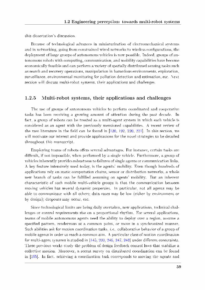
1.2 Engineering perception: towards multi-robot systems
this dissertation's discussion.
Because of technological advances in miniaturization of electromechanical systemsand in networking, going from constrained wired networks to wireless congurations, thedeployment of large groups of autonomous vehicles is now possible. Indeed, groups of au-tonomous robots with computing, communication, and mobility capabilities have becomeeconomically feasible and can perform a variety of spatially distributed sensing tasks suchas search and recovery operations, manipulation in hazardous environments, exploration,surveillance, environmental monitoring for pollution detection and estimation, etc. Nextsection will discuss multi-robot systems, their applications and challenges.
1.2.5 Multi-robot systems, their applications and challenges
The use of groups of autonomous vehicles to perform coordinated and cooperativetasks has been receiving a growing amount of attention during the past decade. Infact, a group of robots can be treated as a multi-agent system in which each vehicle isconsidered as an agent with the previously mentioned capabilities. A recent review ofthe vast literature in the eld can be found in [120, 192, 220, 221]. In this section, wewill motivate our interest and provide applications for the novel strategies to be detailedthroughout this manuscript.
Employing teams of robots oers several advantages. For instance, certain tasks aredicult, if not impossible, when performed by a single vehicle. Furthermore, a group ofvehicles inherently provides robustness to failures of single agents or communication links.A key feature intensively used today, is the agents' mobility. Even though hundreds ofapplications rely on static computation chains, sensor or distribution networks, a wholenew branch of tasks can be fullled assuming on agents' mobility. But an inherentcharacteristic of such mobile multi-vehicle groups is that the communication betweenmoving vehicles has several dynamic properties. In particular, not all agents may beable to communicate with all others; data rates may be low (either by environment orby design); dropouts may occur, etc.
Since technological limits are being daily overtaken, new applications, technical chal-lenges or control requirements rise on a proportional rhythm. For several applications,teams of mobile autonomous agents need the ability to deploy over a region, assume aspecied pattern, rendezvous at a common point, or move in a synchronized manner.Such abilities ask for motion coordination tasks, i.e., collaborative behavior of a group ofmobile agents in order to reach a common aim. A particular class of motion coordinationfor multi-agent systems is studied in [145, 200, 246, 247, 248] under dierent constraints.These previous works study the problem of design feedback control laws that stabilize acollective motion. Moreover, a recent survey on distributed coordination can be foundin [165]. In fact, achieving a coordination task corresponds to moving the agents and
59
Chapter 1. Introduction
changing their state to maximize or minimize an objective function. Furthermore, coor-dination tasks must often be achieved with minimal communication between agents and,therefore, with limited information about the system.
Another important point concerns the interest/need to use a group of vehicles in-stead of one complex, expensive and high capability system. A major advantage is thata group of agents is able to realize tasks that can not easily be achieved by a single vehi-cle. As an example, search/recovey operations, specially in high seas, generally concernan enormous area of terrain to be thoroughly examined. It could take months, evenyears, to nd what so ever if one single agent is deployed. Further, and related withthe decentralized characteristics of the control strategy, a group of vehicles inherentlyprovides robustness to failures of single agents or communication links. All previous top-ics motivate our interest in multi-robot systems, enhancing their numerous advantages.They also provide us insights on control and design of large scaled systems. We are nowgoing to identify several challenging and useful applications for which the work presentedin this manuscript is pertinent and can be easily applied to.
This thesis is related to the European project FeedNetBack 1 supported by the Euro-pean Commission and the French project Connect 2 supported by the Agence Nationalede la Recherche (ANR). Both projects deal with networked control systems, with a spe-cial attention on multi-agent systems and their challenges. Moreover, some contributionsof this manuscript also concern the GDRI DelSys, supported by the Centre National dela Recherche Scientique (CNRS). In particular, the European FeedNetBack involvesnot only several academic partners, but also industrial participants in order to carryout the technological applications. One of the academic participants is the INRIA, andspecically the Networked Control System Team (NeCS) 3 with which this thesis wascarried out. More precisely, NeCS is a joint team-projet between INRIA and GrenobleImages Parole Signal Automatique-Laboratoire (GIPSA-lab) whose goal is to develop anew control framework for assessing problems raised by the consideration of new tech-nological low-cost and wireless components, the increase of systems complexity and thedistributed and dynamic location of sensors and actuators. The main objectives ofFeedNetBack are to design and analyse systems composed of several sub-systems, inter-connected by a constrained communication network. More precisely, this project aimsto preserve closed-loop system stability while taking into account shared computationalresources, distributed sensing and/or constraints on the network topology. One of thestudy cases considered in this project involves formation control strategies of heteroge-neous marine vehicles (surface and underwater vehicles such as autonomous crafts, AUVsor underwater gliders) in order to achieve a scientic mission, see [29, 196] for furtherdetails. The main objective of such formation is to carry out a gradient search and fol-
1. www.feednetback.eu2. www.gipsa-lab.inpg.fr/projet/connect3. http://necs.inrialpes.fr
60
1.2 Engineering perception: towards multi-robot systems
lowing an underwater source, the nature of the source might be very dierent, see, e.g.,[33, 34]. To perform missions involving several vehicles, coordinated motion is required,especially when the goal of the mission is sensor driven. However, the challenge is evenbigger when non-identical robots are taken into consideration and when simple modelingdetails can drastically inuence the eciency of the chosen control strategy.
Autonomous robots are being recurrently used to help humans to perform certaintasks with improved performances and in better safety conditions. Over the last decade,unfortunate aerial or even submarine accidents necessitated the use of high-teck technol-ogy either to search for wreckage, to recover survivors or to protect sensitive technology.This brings us to another important source of applications and inherent technologicalchallenges: military operations.
Unmanned vehicles, whether air, land or sea, are one means to get airmen, soldiers,marines and sailors out of harm's way and are most likely a key driver to an upcomingrevolution in military aairs. Indeed, new technology may be able to help answer the criesto reduce casualties resulting from friendly re and collateral damage, as well as assistthe military in performing urban operations. Military robots nd major applicationsin surveillance, reconnaissance, location and destruction of mines, as well as for hostilemilitary operations, see Figure 1.8. Moreover, recent military reports predict that robotsmight someday be sent into a hostile village to locate prisoners, into an earthquake-damaged building to nd victims or onto chemical-spill sites to examine hazardous waste.Moreover, they might also be able to provide, in a near future, technology for protectingborders and safety in cities or and building smarter cities. In fact, some of the mostadvanced army robots carry dozens of sensors, including high-resolution night-visioncameras, 3-D imagers, and acoustic arrays. However, humans are still needed to operatethese vehicles, interpret the data and coordinate tasks among multiple systems [297].Because even if one day we are going to see fully autonomous robots capable of planningand carrying out missions and learning from their experiences, a basic question willremain: How can we equip these robots to make critical decisions on their own?
Without being able to answer all the previously mentioned problems, this thesisproposes solutions to some problems related to motion coordination among multipleindividuals. We are motivated by recognition, recovery and search operations, such as theFeednetback study case or the civil/military missions described before. This manuscriptis focused on distributed agreement strategies to cooperatively command mobile robots,and more precisely, to perform motion coordination based on local couplings [207]. Thenext section will present the objectives of this thesis.
61
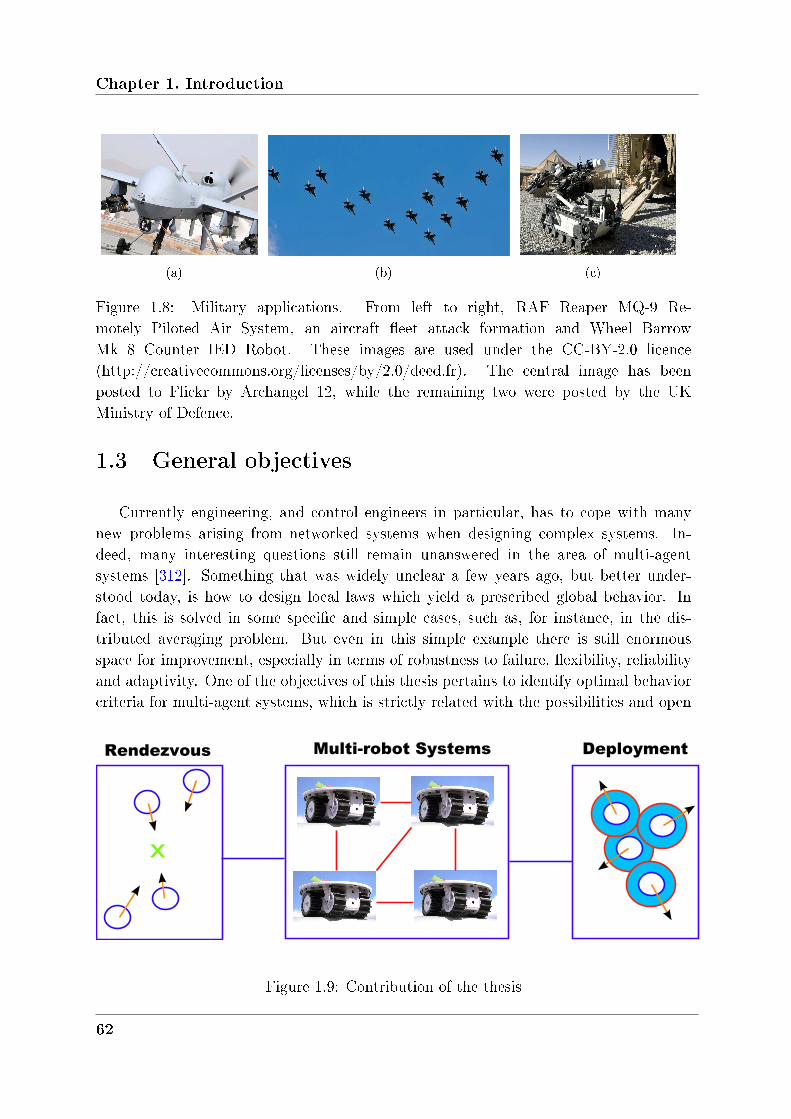
Chapter 1. Introduction
(a) (b) (c)
Figure 1.8: Military applications. From left to right, RAF Reaper MQ-9 Re-motely Piloted Air System, an aircraft eet attack formation and Wheel BarrowMk 8 Counter IED Robot. These images are used under the CC-BY-2.0 licence(http://creativecommons.org/licenses/by/2.0/deed.fr). The central image has beenposted to Flickr by Archangel 12, while the remaining two were posted by the UKMinistry of Defence.
1.3 General objectives
Currently engineering, and control engineers in particular, has to cope with manynew problems arising from networked systems when designing complex systems. In-deed, many interesting questions still remain unanswered in the area of multi-agentsystems [312]. Something that was widely unclear a few years ago, but better under-stood today, is how to design local laws which yield a prescribed global behavior. Infact, this is solved in some specic and simple cases, such as, for instance, in the dis-tributed averaging problem. But even in this simple example there is still enormousspace for improvement, especially in terms of robustness to failure, exibility, reliabilityand adaptivity. One of the objectives of this thesis pertains to identify optimal behaviorcriteria for multi-agent systems, which is strictly related with the possibilities and open
Multi-robot Systems
x
Rendezvous Deployment
Figure 1.9: Contribution of the thesis
62
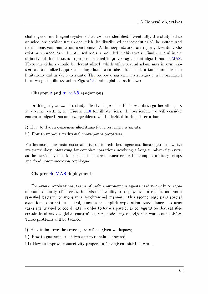
1.3 General objectives
challenges of multi-agents systems that we have identied. Eventually, this study led toan adequate architecture to deal with the distributed characteristics of the system andits inherent communication constraints. A thorough state of art report, describing theexisting approaches and most used tools is provided in this thesis. Finally, the ultimateobjective of this thesis is to propose original/improved agreement algorithms for MAS.These algorithms should be decentralized, which oers several advantages in compari-son to a centralized approach. They should also take into consideration communicationlimitations and model constraints. The proposed agreement strategies can be organizedinto two parts, illustrated in Figure 1.9 and explained as follows:
Chapter 2 and 3: MAS rendezvous
In this part, we want to study eective algorithms that are able to gather all agentsat a same position, see Figure 1.10 for illustrations. In particular, we will considerconsensus algorithms and two problems will be tackled in this dissertation:
i) How to design consensus algorithms for heterogeneous agents;
ii) How to improve traditional convergence properties.
Furthermore, one main constraint is considered: heterogeneous linear systems, whichare particulary interesting for complex operations involving a large number of players,as the previously mentioned scientic search maneuvers or the complex military setupsand xed communication topologies.
Chapter 4: MAS deployment
For several applications, teams of mobile autonomous agents need not only to agreeon some quantity of interest, but also the ability to deploy over a region, assume aspecied pattern, or move in a synchronized manner. This second part pays specialattention to formation control, since to accomplish exploration, surveillance or rescuetasks agents need to coordinate in order to form a particular conguration that satisescertain local and/or global constraints, e.g., node degree and/or network connectivity.Three problems will be tackled:
i) How to improve the coverage rate for a given workspace;
ii) How to guarantee that two agents remain connected;
iii) How to improve connectivity properties for a given initial network.
63
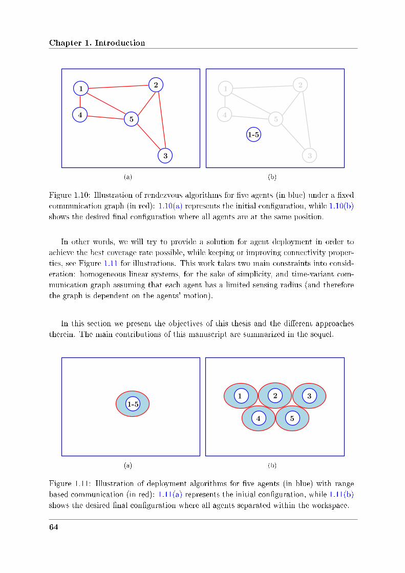
Chapter 1. Introduction
3
2
4
1
5
(a)
3
2
4
1
5
1-5
(b)
Figure 1.10: Illustration of rendezvous algorithms for ve agents (in blue) under a xedcommunication graph (in red): 1.10(a) represents the initial conguration, while 1.10(b)shows the desired nal conguration where all agents are at the same position.
In other words, we will try to provide a solution for agent deployment in order toachieve the best coverage rate possible, while keeping or improving connectivity proper-ties, see Figure 1.11 for illustrations. This work takes two main constraints into consid-eration: homogeneous linear systems, for the sake of simplicity, and time-variant com-munication graph assuming that each agent has a limited sensing radius (and thereforethe graph is dependent on the agents' motion).
In this section we present the objectives of this thesis and the dierent approachestherein. The main contributions of this manuscript are summarized in the sequel.
1-5
(a)
1 2 3
4 5
(b)
Figure 1.11: Illustration of deployment algorithms for ve agents (in blue) with rangebased communication (in red): 1.11(a) represents the initial conguration, while 1.11(b)shows the desired nal conguration where all agents separated within the workspace.
64
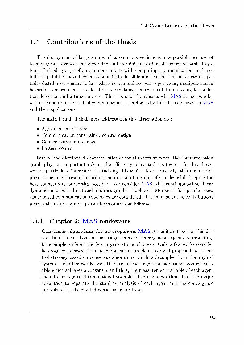
1.4 Contributions of the thesis
1.4 Contributions of the thesis
The deployment of large groups of autonomous vehicles is now possible because oftechnological advances in networking and in miniaturization of electromechanical sys-tems. Indeed, groups of autonomous robots with computing, communication, and mo-bility capabilities have become economically feasible and can perform a variety of spa-tially distributed sensing tasks such as search and recovery operations, manipulation inhazardous environments, exploration, surveillance, environmental monitoring for pollu-tion detection and estimation. etc. This is one of the reasons why MAS are so popularwithin the automatic control community and therefore why this thesis focuses on MASand their applications.
The main technical challenges addressed in this dissertation are:
∙ Agreement algorithms∙ Communication constrained control design∙ Connectivity maintenance∙ Pattern control
Due to the distributed characteristics of multi-robots systems, the communicationgraph plays an important role in the eciency of control strategies. In this thesis,we are particulary interested in studying this topic. More precisely, this manuscriptpresents pertinent results regarding the motion of a group of vehicles while keeping thebest connectivity properties possible. We consider MAS with continuous-time lineardynamics and both direct and undirect graphs' topologies. Moreover, for specic cases,range based communication topologies are considered. The main scientic contributionspresented in this manuscript can be organized as follows.
1.4.1 Chapter 2: MAS rendezvous
Consensus algorithms for heterogenous MAS A signicant part of this dis-sertation is focused on consensus algorithms for heterogeneous agents, representing,for example, dierent models or generations of robots. Only a few works considerheterogeneous cases of the synchronization problem. We will propose here a con-trol strategy based on consensus algorithms which is decoupled from the originalsystem. In other words, we attribute to each agent an additional control vari-able which achieves a consensus and thus, the measurement variable of each agentshould converge to this additional variable. The new algorithm oers the majoradvantage to separate the stability analysis of each agent and the convergenceanalysis of the distributed consensus algorithm.
65
Chapter 1. Introduction
Improved stability of consensus algorithms for MAS In a second part, wefocus on consensus algorithm convergence rate. In several multi-agent control prob-lems, the convergence properties and speed of the system depend on the algebraicconnectivity of the graph. The algebraic connectivity is an important networkproperty for all the previous systems to reach convergence and it characterizes theconvergence rate. More precisely, the algebraic connectivity is equal to the secondsmallest eigenvalue of L. Accelerating the convergence of distributed agreementalgorithms have been studied in the literature based on two main approaches: op-timizing the weights of the topology-related matrix summarizing the updates ateach node [304], or incorporating memory into the distributed averaging algorithm.This last approach will be studied throughout this manuscript. Even if for mostapplications delays lead to a reduction of performances or even to instability, thereexist some cases where the introduction of a delay in the control loop can help tostabilize a system. This has been studied in [110, 252]. In [252], adding a statesampled component to the control law can be seen as an articial way to manipu-late the eigenvalues of L, by getting them further onto the left part of the complexplan and inherently changing the speed of convergence. In this thesis, the objectiveis to maximize the convergence rate value.
1.4.2 Chapter 3: MAS deployment
The third chapter addresses the design and analysis of an algorithm for compactagent deployment. In our approach, the desired formation is specied entirely by anglesformed by agents within the formation. We propose a completely distributed and leader-less algorithm, only based on relative positions that allows swarm self-organization. Therst contribution corresponds to an extension of [76] for swarms dispersion, by adding aconnectivity maintenance force. The second contribution consists of direct angle controlusing only relative positions, which, at the best of our knowledge, has not been pro-posed in literature. This is motivated by the fact that for successful network operations,the deployment should result in congurations that not only provide good environmentcoverage but also satisfy certain local (e.g. node degree) and/or global (e.g. networkconnectivity) constraints. Thus, we intend to minimize inter-agent angles in order toachieve the most compact conguration possible. Note that the minimization of inter-agent angles can also be seen as a maximization or maintenance of node degree. Finally,we also propose a sequential control strategy gathering the two components, showingthat such framework corresponds to a hybrid system.
The ultimate objective of this thesis is to provide pertinent solutions to some of theopen problems of multi-robot systems. We are now ready to present our results.
66
Chapter 2
Consensus strategies for heterogeneous
multi-agent systems
Contents
2.1 Context . . . . . . . . . . . . . . . . . . . . . . . . . . . . . . . 68
2.2 Problem statement and preliminaries . . . . . . . . . . . . . 71
2.3 Controllers design . . . . . . . . . . . . . . . . . . . . . . . . . 72
2.3.1 Local control law . . . . . . . . . . . . . . . . . . . . . . . . . . 73
2.3.2 Distributed consensus algorithm . . . . . . . . . . . . . . . . . 74
2.4 Stability analysis . . . . . . . . . . . . . . . . . . . . . . . . . . 76
2.5 Extensions to more complex situations . . . . . . . . . . . . . 78
2.5.1 Consensus algorithms with transmission delays . . . . . . . . . 79
2.5.2 Consensus algorithms with external reference . . . . . . . . . . 80
2.6 Simulation results . . . . . . . . . . . . . . . . . . . . . . . . . 82
2.7 Conclusions . . . . . . . . . . . . . . . . . . . . . . . . . . . . . 87
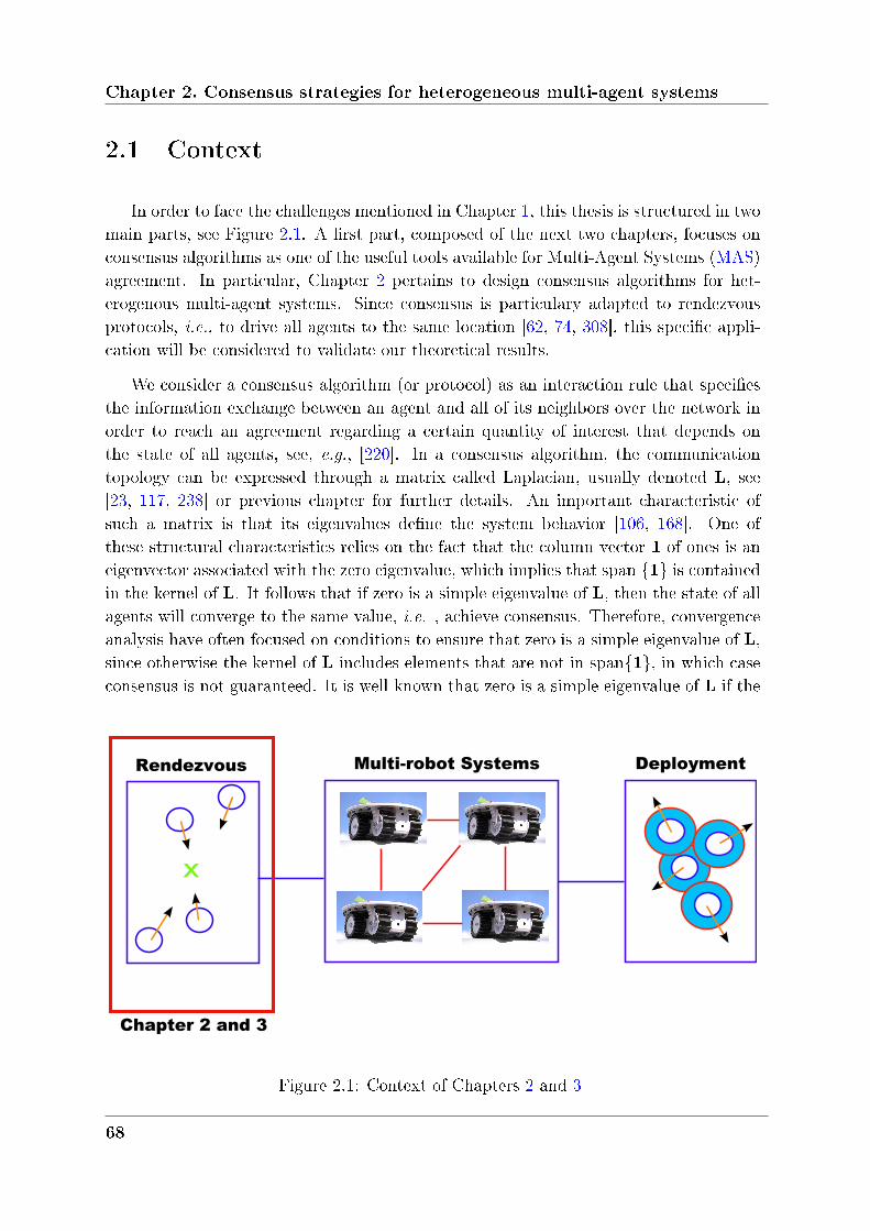
Chapter 2. Consensus strategies for heterogeneous multi-agent systems
2.1 Context
In order to face the challenges mentioned in Chapter 1, this thesis is structured in twomain parts, see Figure 2.1. A rst part, composed of the next two chapters, focuses onconsensus algorithms as one of the useful tools available for Multi-Agent Systems (MAS)agreement. In particular, Chapter 2 pertains to design consensus algorithms for het-erogenous multi-agent systems. Since consensus is particulary adapted to rendezvousprotocols, i.e., to drive all agents to the same location [62, 74, 308], this specic appli-cation will be considered to validate our theoretical results.
We consider a consensus algorithm (or protocol) as an interaction rule that speciesthe information exchange between an agent and all of its neighbors over the network inorder to reach an agreement regarding a certain quantity of interest that depends onthe state of all agents, see, e.g., [220]. In a consensus algorithm, the communicationtopology can be expressed through a matrix called Laplacian, usually denoted L, see[23, 117, 238] or previous chapter for further details. An important characteristic ofsuch a matrix is that its eigenvalues dene the system behavior [106, 168]. One ofthese structural characteristics relies on the fact that the column vector 1 of ones is aneigenvector associated with the zero eigenvalue, which implies that span 1 is containedin the kernel of L. It follows that if zero is a simple eigenvalue of L, then the state of allagents will converge to the same value, i.e. , achieve consensus. Therefore, convergenceanalysis have often focused on conditions to ensure that zero is a simple eigenvalue of L,since otherwise the kernel of L includes elements that are not in span1, in which caseconsensus is not guaranteed. It is well-known that zero is a simple eigenvalue of L if the
Multi-robot Systems
x
Rendezvous Deployment
Chapter 2 and 3
Figure 2.1: Context of Chapters 2 and 3
68
2.1 Context
graph of L is strongly connected [54]. However, this is only a sucient condition ratherthan a necessary one. Based on an induction approach, the formal statement that zero isa simple eigenvalue of the Laplacian matrix if and only if its digraph has a spanning treehas been shown in [223]. Furthermore, the same result is proven independently in [155] bya constructive approach. Consequently, it follows that under a time invariant informationexchange topology, the continuous time protocol asymptotically achieves consensus if andonly if the information exchange topology has a spanning tree. In a parallel way, but outof the scope of this manuscript, several works consider discrete time consensus algorithms[127, 174, 219, 324]. In fact, the well-known Perron-Frobenius theorem states that oneis a simple eigenvalue of a stochastic matrix (used in an equivalent way as the Laplacianmatrix) if the corresponding graph is strongly connected which, as for the continuoustime case, is only a sucient condition rather than a necessary one. Consequently, theauthors of [219] prove that for a stochastic matrix, one is a unique eigenvalue of modulusone if and only if its digraph has a spanning tree.
There exist a huge number of contributions to this problem including: communica-tion delays in [46, 69, 173, 194, 304], nonlinear consensus protocols in [14, 194, 258],stochastic algorithms in [113] or tracking of linear consensus on time-varying inputs in[262], among many others [40, 192, 195, 219, 251]. Furthermore, although consensusproblems are signicantly simplied by assuming a time-invariant information exchangetopology, the information exchange topology between agents may change dynamicallyin reality. For instance, communication links between agents may be unreliable due todisturbances and/or subject to communication range limitations [31, 71, 78, 87, 240].If information is being exchanged by direct sensing, the locally visible neighbors of anagent will likely change over time. Based on a particular model introduced in [294],which is a special case of the distributed behavioral model proposed by Reynold's in[227], many researchers worked on coordination of multiple autonomous agents underswitching information exchange topologies, see [46, 128, 127, 154, 219, 239, 319] or [258]using nonlinear contraction theory.
Consensus algorithms are extensively studied in the literature for identical multi-agent systems [154, 173, 194, 241, 248] and in particular to simple and double integratordynamics, see, for instance, [194, 220] and the references therein. However, increasinginterest has turned to MAS with general linear time-invariant dynamical agents, see,e.g., [89, 242, 298].
In this chapter, we are interested in consensus algorithms for heterogeneous multi-agent systems, i.e., with non-identical dynamics representing, for example, dierentmodels or generations of robots. For a system consisting of heterogeneous dynamicalagents, the rst question to be answered is whether there exist a consensus solution tosuch a system. Only a few papers consider heterogeneous cases of the synchronizationproblem. In particular, [51, 211] solved the output synchronization problem under a non
69
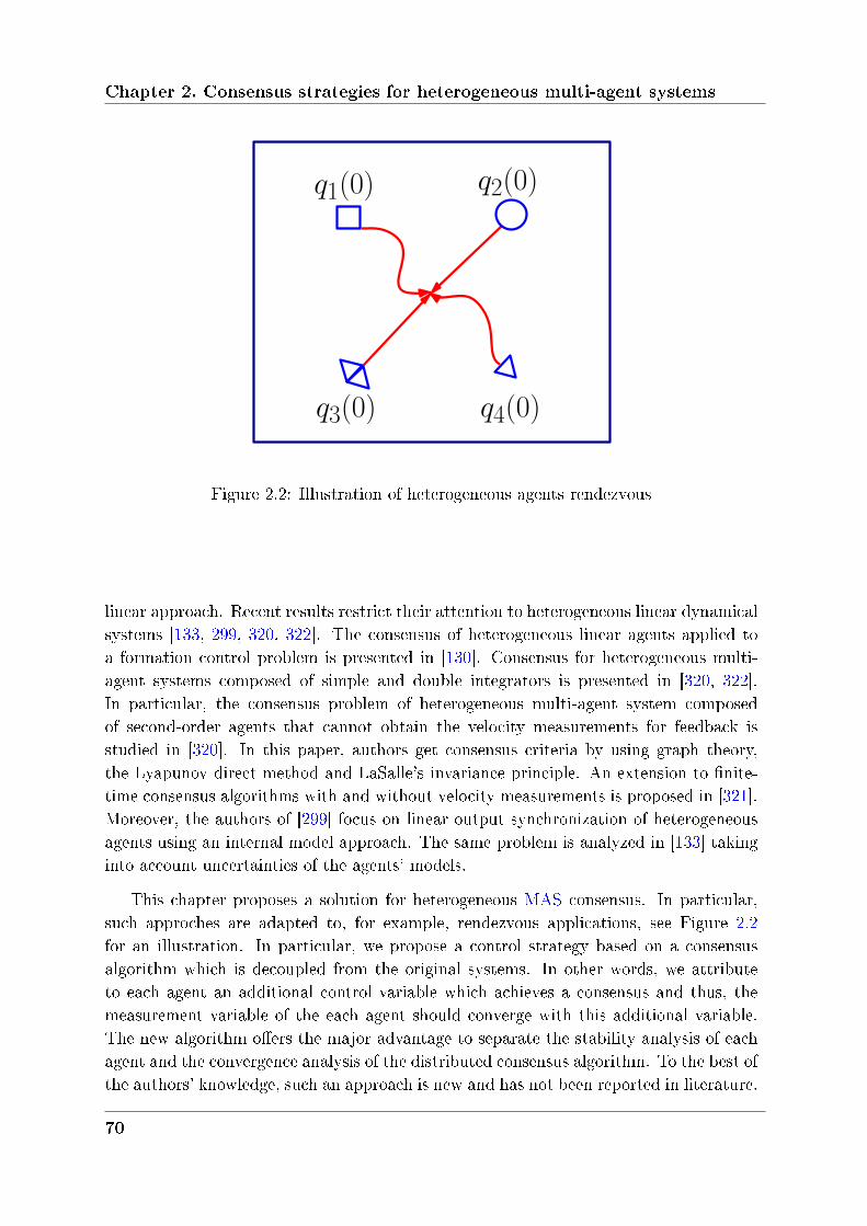
Chapter 2. Consensus strategies for heterogeneous multi-agent systems
q1(0) q2(0)
q3(0) q4(0)
Figure 2.2: Illustration of heterogeneous agents rendezvous
linear approach. Recent results restrict their attention to heterogeneous linear dynamicalsystems [133, 299, 320, 322]. The consensus of heterogeneous linear agents applied toa formation control problem is presented in [130]. Consensus for heterogeneous multi-agent systems composed of simple and double integrators is presented in [320, 322].In particular, the consensus problem of heterogeneous multi-agent system composedof second-order agents that cannot obtain the velocity measurements for feedback isstudied in [320]. In this paper, authors get consensus criteria by using graph theory,the Lyapunov direct method and LaSalle's invariance principle. An extension to nite-time consensus algorithms with and without velocity measurements is proposed in [321].Moreover, the authors of [299] focus on linear output synchronization of heterogeneousagents using an internal model approach. The same problem is analyzed in [133] takinginto account uncertainties of the agents' models.
This chapter proposes a solution for heterogeneous MAS consensus. In particular,such approches are adapted to, for example, rendezvous applications, see Figure 2.2for an illustration. In particular, we propose a control strategy based on a consensusalgorithm which is decoupled from the original systems. In other words, we attributeto each agent an additional control variable which achieves a consensus and thus, themeasurement variable of the each agent should converge with this additional variable.The new algorithm oers the major advantage to separate the stability analysis of eachagent and the convergence analysis of the distributed consensus algorithm. To the best ofthe authors' knowledge, such an approach is new and has not been reported in literature.
70
2.2 Problem statement and preliminaries
2.2 Problem statement and preliminaries
Assuming systems composed of heterogenous agents representing, for example, dif-ferent models or generations of robots, oer major advantages specially in terms ofscalability and/or modularity. Moreover, such a setup naturally ts into several chal-lenging applications relying, for instance, on surface and underwater marine vehiclesor on ground and aerial robots. Consequently, this work is motivated by recognition,recovery and search operations on a civil or military framework.
Consider a graph 𝒢 with 𝑁 agents and an edge set given by 𝐸 = (𝑖, 𝑗) : 𝑗 ∈ 𝒩𝑖.Based on Chapter 1's concepts, the adjacency matrix 𝒜 = 𝒜(𝐺) = (𝑎𝑖𝑗) is a 𝑁 × 𝑁
matrix given by 𝑎𝑖𝑗 = 1, if (𝑖, 𝑗) ∈ 𝐸 and 𝑎𝑖𝑗 = 0, otherwise. If there is an edge connectingtwo vertices 𝑖, 𝑗, i.e.,(𝑖, 𝑗) ∈ 𝐸, then 𝑖, 𝑗 are called adjacent. The degree 𝑑𝑖 of vertex 𝑖is dened as the number of its neighboring vertices, i.e., 𝑑𝑖 = #𝑗 : (𝑖, 𝑗) ∈ 𝐸. Denotealso 𝑑𝑚𝑎𝑥 = 𝑚𝑎𝑥𝑑𝑖. Let ∆ be the 𝑁 × 𝑁 diagonal matrix of 𝑑𝑖's. Furthermore, theLaplacian of 𝒢 is the matrix 𝐿 = ∆ −𝒜.
In the scope of multi-robots systems, we are particulary motivated by motion controlin a cartesian plane. Consequently, the position of each agent 𝑖 is denoted:
𝑞𝑖 = [𝑥𝑖, 𝑦𝑖]𝑇 ∈ R2,
where 𝑥𝑖 and 𝑦𝑖 represent the dynamics of 𝑞𝑖 on the x-axis and y-axis, respectively.However, for the sake of notation's clearness and without loss of generality, in this chapterwe consider only the dynamics of 𝑥𝑖. Thus, consider the following multi-agent linearsystem: ⎧⎪⎨⎪⎩
𝑖 = 𝐴𝑖𝑥𝑖 +𝐵𝑖𝑢𝑖
𝑦𝑖 = 𝑥𝑖
𝑧𝑖 = 𝐶𝑖𝑥𝑖
∀𝑖 ∈ 𝒩 = 1, . . . , 𝑁, (2.2.1)
where 𝑥𝑖 ∈ R𝑛𝑖 , 𝑦𝑖 ∈ R𝑛𝑖 , 𝑧𝑖 ∈ R𝑚 and 𝑢𝑖 ∈ R𝑚 are the state, output, measurementand input vectors, respectively. Note that it is assumed that the state of the system isavailable for the design of the controller, i.e., 𝑦𝑖 = 𝑥𝑖 for all 𝑖 ∈ 𝒩 . For all 𝑖 ∈ 𝒩 , thematrices 𝐴𝑖 ∈ R𝑛𝑖×𝑛𝑖 , 𝐵𝑖 ∈ R𝑛𝑖×𝑚 and 𝐶𝑖 ∈ R𝑚×𝑛𝑖 , with 𝑚 < min𝑛𝑖 and 𝑛𝑖 > 𝑚 areassumed to be constant and known.
In this context, the objective is the design of a distributed control law ensuring that(i) each subsystem is stable and (ii) the measurement vectors of each agent reach anagreement. To deal with these problems, the following assumptions on the systems areconsidered:
71
Chapter 2. Consensus strategies for heterogeneous multi-agent systems
Assumption 2.1. (Heterogeneity): The 𝑁 systems are assumed to be heterogeneous.
In other words, this simply means that the matrices dening the systems may dierfrom one agent to another one and that the vectors 𝑥𝑖 may have dierent dimensions.
Assumption 2.2. (Homogeneity of the measurement vector): The measurement
vectors 𝑧𝑖 represents the same quantity of interests for all agents. As a consequence, the
measurement vectors have the same dimension, or in other words, 𝑧𝑖 ∈ R𝑚 ∀𝑖 ∈ 𝒩 ,
where 𝑚 < min𝑛𝑖.
Assumption 2.3. (Structures of the systems): For all 𝑖 ∈ 𝒩 , the condition
𝑟𝑎𝑛𝑘(𝐶𝑖𝐵𝑖) = 𝑚 holds.
Technically speaking, it means that the input vectors directly aect the measurementvector.
Assumption 2.4. (Controllability): For each agent, the pair (𝐴𝑖, 𝐵𝑖) is controllable.
In order to avoid a centralized solution of the problem, the agents are assumed to beconnected through a communication network. To establish further stability results, thefollowing assumption holds.
Assumption 2.5. (Graph’s connectivity): For any considered graph 𝐺, we assume
that the communication graph has a directed spanning tree.
This ensures that zero is a simple eigenvalue of L and the corresponding eigenvector isthe vector of ones,
−→1 . Consequently, it implies that the algorithm will eventually reach
consensus. Note that requiring a directed spanning tree is considerably less stringentthan requiring a strongly connected and balanced graph [220].
The objective is to design an eective agreement strategy for heterogenous multi-agent systems. We propose here a control strategy based on trivial consensus algorithmswhich is decoupled from the original systems. In other words, we attribute to each agentan additional control variable which achieves a consensus such that the measurementvariable of each agent should converge with this additional variable. The exact controlobjectives and needed assumptions have just been introduced. Next section presents thecontrol design for arbitrary heterogeneous agents.
2.3 Controllers design
In order to achieve the goals mentioned above, a controller composed of two parts,one corresponding to the local controller and one representing the consensus algorithm,
72
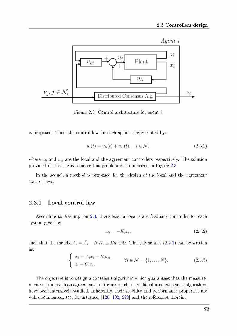
2.3 Controllers design
Plant
uli
uci
Distributed Consensus Alg.
++
zi
xi
νiνj, j ∈ Ni
Agent i
ui
Figure 2.3: Control architecture for agent 𝑖
is proposed. Thus, the control law for each agent is represented by:
𝑢𝑖(𝑡) = 𝑢𝑙𝑖(𝑡) + 𝑢𝑐𝑖(𝑡), 𝑖 ∈ 𝒩 . (2.3.1)
where 𝑢𝑙𝑖 and 𝑢𝑐𝑖 are the local and the agreement controllers respectively. The solutionprovided in this thesis to solve this problem is summarized in Figure 2.3.
In the sequel, a method is proposed for the design of the local and the agreementcontrol laws.
2.3.1 Local control law
According to Assumption 2.4, there exist a local state feedback controller for eachsystem given by:
𝑢𝑙𝑖 = −𝐾𝑖𝑥𝑖, (2.3.2)
such that the matrix 𝐴𝑖 = 𝐴𝑖 −𝐵𝑖𝐾𝑖 is Hurwitz. Thus, dynamics (2.2.1) can be writtenas:
𝑖 = 𝐴𝑖𝑥𝑖 +𝐵𝑖𝑢𝑐𝑖,
𝑧𝑖 = 𝐶𝑖𝑥𝑖,∀𝑖 ∈ 𝒩 = 1, . . . , 𝑁. (2.3.3)
The objective is to design a consensus algorithm which guarantees that the measure-ment vectors reach an agreement. In literature, classical distributed consensus algorithmshave been intensively studied. Inherently, their stability and performance properties arewell documented, see, for instance, [120, 192, 220] and the references therein.
73
Chapter 2. Consensus strategies for heterogeneous multi-agent systems
2.3.2 Distributed consensus algorithm
In this section, we aim to design a consensus protocol which ensures that the measure-ment vectors reach an agreement. In literature, classical distributed consensus algorithmshave been intensively studied. To achieve agents' agreement, consensus algorithms basedon simple integrator dynamics [13, 194, 251] have been widely considered and appliedto dierent applications for MAS such as formation control [171], rendezvous [62], cyclepursuit [134, 161], coverage [63, 206, 243] among many others [111, 127]. Inherently, thestability and performance properties of these simple controllers are well documented, forinstance in [120, 192, 220] and the references therein.
One can easily realize that the control complexity for systems considering heteroge-neous agents is greater than for simpler frameworks. Furthermore, even though someresults for such a problem have been proposed in literature, most of them present majordrawbacks such as calculation needs, complexity or accuracy of the solution. To over-take heterogeneous MAS agreement issues, we were able to propose an ecient way tosimplify the control design. More precisely, the main idea is to add additional dynamicsto the control law of each system which correspond to a trivial consensus algorithm. Asa starting point, we will consider the simplest situation where the dynamics of theseadditional dynamics are driven by:
𝑖 = −∑𝑗∈𝒩𝑖
(𝜈𝑖 − 𝜈𝑗), ∀𝑖 ∈ 𝒩 , (2.3.4)
where 𝜈𝑖 ∈ R𝑚. This allows dening the augmented vector 𝜈 = [𝜈1, . . . , 𝜈𝑁 ]𝑇 and thus theprevious consensus algorithm can be rewritten in a matrix form such as = −L⊗ 𝐼𝑚𝜈,where L is the Laplacian matrix associated to the communication graph of the multiagent system and ⊗ represents the classical Kronecker product.
The stability of such a system has been widely studied in literature. See, for exam-ple, [192, 220] among many others. The well known convergence properties of (2.3.4)naturally motivate it as an appropriated "choice" for the additional dynamics. The restof the contribution consists on using this well known consensus algorithm to reach anagreement on those additional dynamics, while applying a standard model tracking basedcontroller to the remaining system. This ensures that the real system will have identicalperformances as the additional model. Due to the interactions between them, 𝑢𝑐𝑖 mustbe designed in a proper manner such that two correlated objectives are fullled:⎧⎨⎩ lim
𝑡→∞(𝜈𝑖 − 𝜈𝑗) = 0,
lim𝑡→∞
(𝑧𝑖 − 𝜈𝑖) = 0,∀𝑖, 𝑗 ∈ 𝒩 2. (2.3.5)
In other words, system (2.3.4) can then be seen as a reference model for system (2.2.1).Then, it is natural to introduce the error vector between the measurement vector 𝑧
74
2.3 Controllers design
from (2.2.1) and the additional dynamics 𝜈 given by:
𝜀𝑖 = 𝑧𝑖 − 𝜈𝑖. (2.3.6)
We wish to ensure that each 𝜀𝑖 converges to zero as the time evolves. Therefore, theevolution of 𝜀𝑖 has the following dynamics:
𝑖 = −𝛽𝜀𝑖,
where 𝛽 > 0. Thus, it follows:
𝑖 − 𝑖 = −𝛽(𝑧𝑖 − 𝜈𝑖),
𝐶𝑖(𝐴𝑖𝑥𝑖 +𝐵𝑖𝑢𝑐𝑖) + (L)𝑖 ⊗ 𝐼𝑚𝜈 = −𝛽𝜀, (2.3.7)
where (L)𝑖 denotes the 𝑖𝑡ℎ line of the matrix L. Due to the Assumption 2.3, 𝐶𝑖𝐵𝑖 isinvertible for all agent 𝑖, and thus the proposed controller can be expressed as a standardasymptotic output tracking controller, see [126]. Therefore, it yields:
𝑢𝑐𝑖 = (𝐶𝑖𝐵𝑖)−1 (𝑖 − 𝛽(𝑧𝑖 − 𝜈𝑖) − 𝐶𝑖𝐴𝑖𝑥𝑖) . (2.3.8)
Remark 2.1. One might see that in the previous calculus we inherently assume that,
at each time instant, each agent 𝑖 has access to its own full state. Despite the fact
that, theoretical speaking, this does not represent a too conservative condition, the same
comment does not hold in terms of practical application. However, this assumption might
be relaxed by applying a observer and using the estimated state instead. For the sake of
brevity, though, the synthesis of this observer will not be considered in this dissertation.
Relying on a decoupling approach as well, a solution to the output synchronizationproblem for heterogeneous agents is presented in [299]. In particular, authors showedthat an internal model requirement is necessary and sucient for exponential synchroniz-ability of a group of heterogeneous agents. Following [242], the authors add an internalmodel to the dynamics of each agent and synchronize these identical exosystems suchthat an output synchronization of the multi-agent systems is achieved. In order to com-pensate for heterogeneity in the individual system's dynamics, authors proposed in [299]specic coupling dynamics that are composed of (i) synchronized reference generators;(ii) Luenberger observers and (iii) static output regulation controllers. Therefore, eachagent solves an output regulation problem with respect to its attached exosystem andthe output synchronization problem for heterogeneous multi-agent systems is split intotwo parts: a homogeneous synchronization problem and local output regulation problem.Furthermore, these results can be easily extended to the case when reference generatorscontain exponentially unstable modes by imposing stronger connectedness assumptionsonto the communication graph [242].
75
Chapter 2. Consensus strategies for heterogeneous multi-agent systems
Our objective is to obtain a very simple control technique to reach consensus ofheterogeneous multi-agent systems. In this chapter, the synchronization problem cor-responds to single-integrator consensus and the output regulation problem is solved byan asymptotic output tracking controller due to the special structure of the agents un-der consideration, see Assumption 2.3. The main dierence with respect to [299] isthat the heterogeneous synchronization problem is solved using the properties of simple-integrator consensus algorithms. Consequently, this approach can easily be extended tomore complex and realistic situations where, for instance, communication delays or ex-ternal references are considered. Moreover, this structure seems to considerably reducethe control complexity and computational eorts with respect to [299].
The previous section presented and motivated the proposed control strategy. In thesequel we are going to provide stability conditions for this framework.
2.4 Stability analysis
In this section we are going to present stability conditions for the closed-loop multi-agent system (2.2.1) controlled by (2.3.1). This analysis oers the major advantage ofseparated stability analysis of each agent and the convergence analysis of the distributedconsensus algorithm. The next theorem states our main result:
Theorem 2.1. (Rodrigues de Campos et al. [228]) If Assumptions 2.1-5 are satisfied,
then the control law (2.3.1), given by:
𝑢𝑖 = −𝐾𝑖𝑥𝑖 + (𝐶𝑖𝐵𝑖)−1 (𝑖 − 𝛽(𝑧𝑖 − 𝜈𝑖) − 𝐶𝑖𝐴𝑖𝑥𝑖) (2.4.1)
where 𝑖 is given by (2.3.4), guarantees that the multi-agent system (2.2.1) is stable andreaches an asymptotic measurement variable consensus, i.e., 𝑧𝑖 = 𝑧𝑗, ∀𝑖, 𝑗 ∈ 𝒩 .
Proof. In order to consider measurement variable consensus, an appropriate canonicalrepresentation of the locally controlled system is presented in the sequel following [6,82, 83]. Consider that Assumption 2.3 is fullled and without loss of generality that𝐶 =
[0 𝐼𝑚
]. The input distribution matrix can be partitioned in such a way that:
𝐵𝑖 =
[1𝑖
2𝑖
],
where 1𝑖 ∈ R(𝑛𝑖−𝑚)×𝑚 and 2𝑖 ∈ R𝑚×𝑚. Then 𝐶𝐵 = 2𝑖 and under Assumption 2.3𝑟𝑎𝑛𝑘(2𝑖) = 𝑚. Hence, in particular, the left pseudo-inverse *
2𝑖 = (𝑇2𝑖2𝑖)
−1𝑇2𝑖 is well
dened and there exist an orthogonal matrix 𝑇𝑖 ∈ R𝑚×𝑚 such that:
76
2.4 Stability analysis
𝑇𝑖2𝑖 =
[0
𝐵2𝑖
],
where 𝐵2𝑖 ∈ R𝑚×𝑚 is non-singular. Therefore, with 𝜒𝑖 ∈ R𝑛𝑖−𝑚 and 𝑇𝑖 ∈ R𝑚×𝑚, thereexist a coordinate transformation of the form:[
𝜒𝑖𝑧𝑖
]= 𝑇𝑖𝑥𝑖, (2.4.2)
where 𝑇𝑖 is given by:
𝑇𝑖 =
[𝐼𝑛𝑖−𝑚 −1𝑖
*2𝑖
0 𝑇𝑖𝑇
].
With respect to the new coordinated, the input distribution matrix is now given by:
𝐵𝑖 =
[0
𝐵2𝑖
],
and the output distribution matrix by:
𝐶𝑖 =[
0 𝑇𝑖].
Under the variable transformation (2.4.2), the new system matrix can be partitioned asfollows:
𝑇𝑖𝐴𝑖𝑇−1𝑖 =
[𝐴11𝑖 𝐴12𝑖
𝐴21𝑖 𝐴22𝑖
],
and consequently, each system (2.3.3) can be rewritten as:[𝑖𝑖
]=
[𝐴11𝑖 𝐴12𝑖
𝐴21𝑖 𝐴22𝑖
] [𝜒𝑖𝑧𝑖
]+
[0
𝐵2𝑖
]𝑢𝑐𝑖, (2.4.3)
where 𝜒𝑖 ∈ R𝑛𝑖−𝑚. Note that in this new representation, 𝐴11𝑖 ∈ R(𝑛𝑖−𝑚)×(𝑛𝑖−𝑚) isHurwitz, 𝐴22𝑖 ∈ R𝑚×𝑚 and 𝐵2𝑖 ∈ R𝑚×𝑚 is invertible. Further details and extensions to,for example, observability canonical forms can be found in [82] or [83]. The system is nowrewritten in an appropriate canonical form particulary useful to consider the problemof measurement variable consensus. Due to previous transformations, the control law(2.4.1) can be rewritten as follows:
𝑢𝑖 = −𝐾𝑖𝑥𝑖 +𝐵−12𝑖 [𝑖 − 𝛽(𝑧𝑖 − 𝜈𝑖) − [0 𝐼𝑚]𝑇𝑖𝐴𝑖𝑥𝑖] . (2.4.4)
77
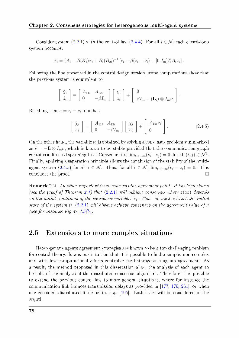
Chapter 2. Consensus strategies for heterogeneous multi-agent systems
Consider system (2.2.1) with the control law (2.4.4). For all 𝑖 ∈ 𝒩 , each closed-loopsystem becomes:
𝑖 = (𝐴𝑖 −𝐵𝑖𝐾𝑖)𝑥𝑖 +𝐵𝑖(𝐵2𝑖)−1 [𝑖 − 𝛽(𝑧𝑖 − 𝜈𝑖) − [0 𝐼𝑚]𝑇𝑖𝐴𝑖𝑥𝑖] .
Following the line presented in the control design section, some computations show thatthe previous system is equivalent to:[
𝑖𝑖
]=
[𝐴11𝑖 𝐴12𝑖
0 −𝛽𝐼𝑚
] [𝜒𝑖𝑧𝑖
]+
[0
𝛽𝐼𝑚 − (L𝑖) ⊗ 𝐼𝑚𝜈
].
Recalling that 𝜀 = 𝑧𝑖 − 𝜈𝑖, one has:[𝑖𝑖
]=
[𝐴11𝑖 𝐴12𝑖
0 −𝛽𝐼𝑚
] [𝜒𝑖𝜀𝑖
]+
[𝐴12𝑖𝜈𝑖
0
]. (2.4.5)
On the other hand, the variable 𝜈𝑖 is obtained by solving a consensus problem summarizedas = −L⊗ 𝐼𝑚𝜈, which is known to be stable provided that the communication graphcontains a directed spanning tree. Consequently, lim𝑡→+∞(𝜈𝑖−𝜈𝑗) = 0, for all (𝑖, 𝑗) ∈ 𝒩 2.Finally, applying a separation principle allows the conclusion of the stability of the multi-agent system (2.4.5) for all 𝑖 ∈ 𝒩 . Thus, for all 𝑖 ∈ 𝒩 , lim𝑡→+∞(𝜈𝑖 − 𝑧𝑖) = 0. Thisconcludes the proof.
Remark 2.2. An other important issue concerns the agreement point. It has been shown
(see the proof of Theorem 2.1) that (2.2.1) will achieve consensus where 𝑧(∞) depends
on the initial conditions of the consensus variables 𝜈𝑖. Thus, no matter which the initial
state of the system is, (2.2.1) will always achieve consensus on the agreement value of 𝜈
(see for instance Figure 2.5(b)).
2.5 Extensions to more complex situations
Heterogenous agents agreement strategies are known to be a top challenging problemfor control theory. It was our intuition that it is possible to nd a simple, non-complexand with low computational eorts controller for heterogenous agents agreement. Asa result, the method proposed in this dissertation allow the analysis of each agent tobe split of the analysis of the distributed consensus algorithm. Therefore, it is possibleto extend the previous control law to more general situations, where for instance thecommunication link induces transmission delays as provided in [177, 179, 251], or whenone considers distributed lters as in, e.g., [195]. Both cases will be considered in thesequel.
78
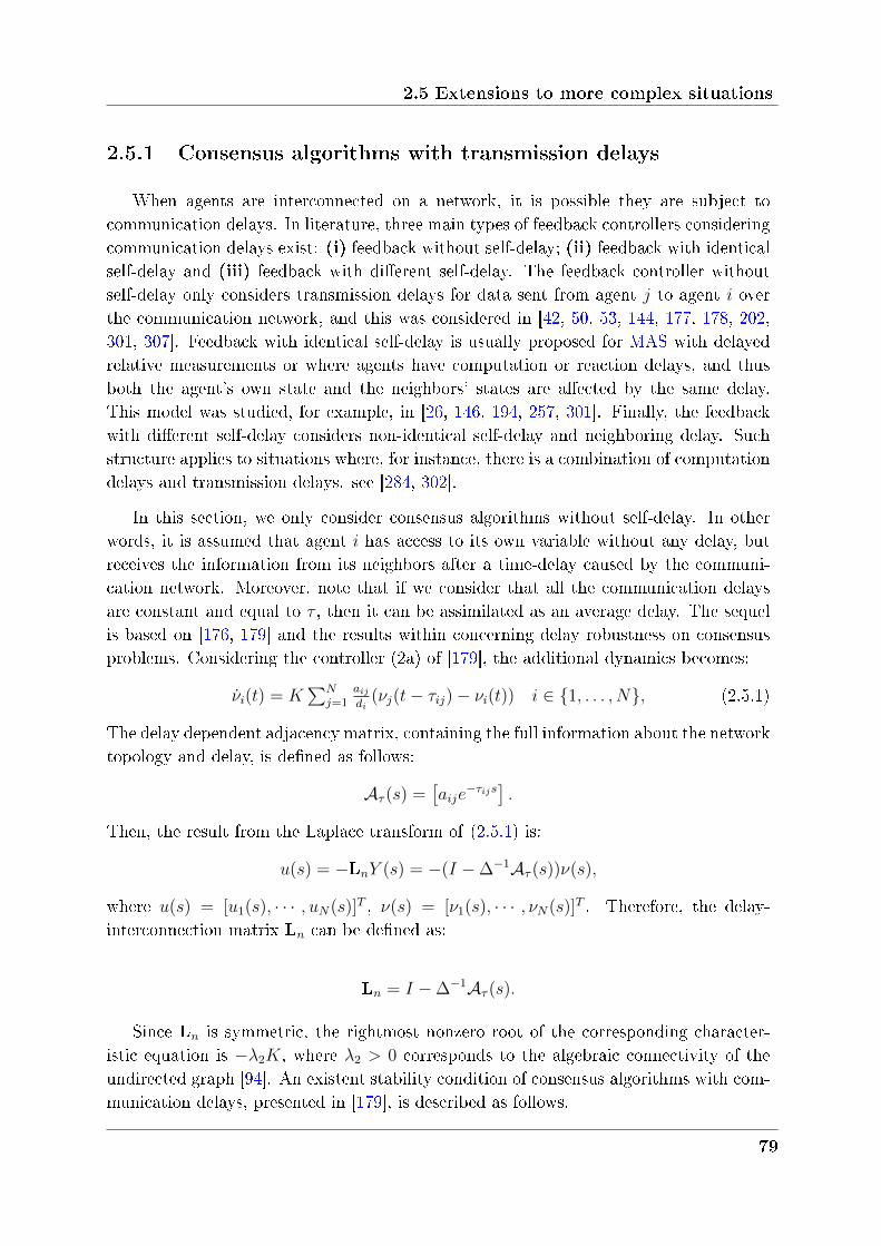
2.5 Extensions to more complex situations
2.5.1 Consensus algorithms with transmission delays
When agents are interconnected on a network, it is possible they are subject tocommunication delays. In literature, three main types of feedback controllers consideringcommunication delays exist: (i) feedback without self-delay; (ii) feedback with identicalself-delay and (iii) feedback with dierent self-delay. The feedback controller withoutself-delay only considers transmission delays for data sent from agent 𝑗 to agent 𝑖 overthe communication network, and this was considered in [42, 50, 53, 144, 177, 178, 202,301, 307]. Feedback with identical self-delay is usually proposed for MAS with delayedrelative measurements or where agents have computation or reaction delays, and thusboth the agent's own state and the neighbors' states are aected by the same delay.This model was studied, for example, in [26, 146, 194, 257, 301]. Finally, the feedbackwith dierent self-delay considers non-identical self-delay and neighboring delay. Suchstructure applies to situations where, for instance, there is a combination of computationdelays and transmission delays. see [284, 302].
In this section, we only consider consensus algorithms without self-delay. In otherwords, it is assumed that agent 𝑖 has access to its own variable without any delay, butreceives the information from its neighbors after a time-delay caused by the communi-cation network. Moreover, note that if we consider that all the communication delaysare constant and equal to 𝜏 , then it can be assimilated as an average delay. The sequelis based on [176, 179] and the results within concerning delay robustness on consensusproblems. Considering the controller (2a) of [179], the additional dynamics becomes:
𝑖(𝑡) = 𝐾∑𝑁
𝑗=1𝑎𝑖𝑗𝑑𝑖
(𝜈𝑗(𝑡− 𝜏𝑖𝑗) − 𝜈𝑖(𝑡)) 𝑖 ∈ 1, . . . , 𝑁, (2.5.1)
The delay dependent adjacency matrix, containing the full information about the networktopology and delay, is dened as follows:
𝒜𝜏 (𝑠) =[𝑎𝑖𝑗𝑒
−𝜏𝑖𝑗𝑠].
Then, the result from the Laplace transform of (2.5.1) is:
𝑢(𝑠) = −L𝑛𝑌 (𝑠) = −(𝐼 − ∆−1𝒜𝜏 (𝑠))𝜈(𝑠),
where 𝑢(𝑠) = [𝑢1(𝑠), · · · , 𝑢𝑁(𝑠)]𝑇 , 𝜈(𝑠) = [𝜈1(𝑠), · · · , 𝜈𝑁(𝑠)]𝑇 . Therefore, the delay-interconnection matrix L𝑛 can be dened as:
L𝑛 = 𝐼 − ∆−1𝒜𝜏 (𝑠).
Since L𝑛 is symmetric, the rightmost nonzero root of the corresponding character-istic equation is −𝜆2𝐾, where 𝜆2 > 0 corresponds to the algebraic connectivity of theundirected graph [94]. An existent stability condition of consensus algorithms with com-munication delays, presented in [179], is described as follows.
79
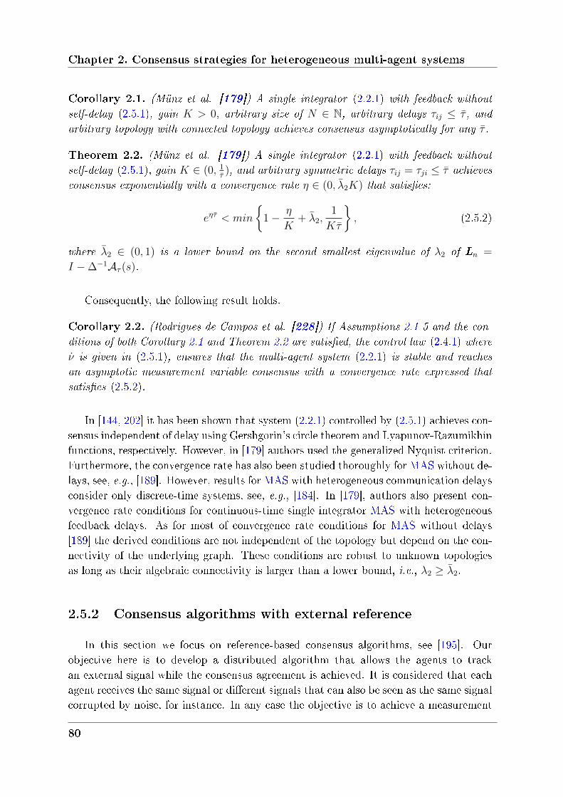
Chapter 2. Consensus strategies for heterogeneous multi-agent systems
Corollary 2.1. (Münz et al. [179]) A single integrator (2.2.1) with feedback without
self-delay (2.5.1), gain 𝐾 > 0, arbitrary size of 𝑁 ∈ N, arbitrary delays 𝜏𝑖𝑗 ≤ 𝜏 , and
arbitrary topology with connected topology achieves consensus asymptotically for any 𝜏 .
Theorem 2.2. (Münz et al. [179]) A single integrator (2.2.1) with feedback without
self-delay (2.5.1), gain 𝐾 ∈ (0, 1𝜏), and arbitrary symmetric delays 𝜏𝑖𝑗 = 𝜏𝑗𝑖 ≤ 𝜏 achieves
consensus exponentially with a convergence rate 𝜂 ∈ (0, 2𝐾) that satisfies:
𝑒𝜂𝜏 < 𝑚𝑖𝑛
1 − 𝜂
𝐾+ 2,
1
𝐾𝜏
, (2.5.2)
where 2 ∈ (0, 1) is a lower bound on the second smallest eigenvalue of 𝜆2 of L𝑛 =
𝐼 − ∆−1𝒜𝜏 (𝑠).
Consequently, the following result holds.
Corollary 2.2. (Rodrigues de Campos et al. [228]) If Assumptions 2.1-5 and the con-
ditions of both Corollary 2.1 and Theorem 2.2 are satisfied, the control law (2.4.1) where is given in (2.5.1), ensures that the multi-agent system (2.2.1) is stable and reaches
an asymptotic measurement variable consensus with a convergence rate expressed that
satisfies (2.5.2).
In [144, 202] it has been shown that system (2.2.1) controlled by (2.5.1) achieves con-sensus independent of delay using Gershgorin's circle theorem and Lyapunov-Razumikhinfunctions, respectively. However, in [179] authors used the generalized Nyquist criterion.Furthermore, the convergence rate has also been studied thoroughly for MAS without de-lays, see, e.g., [189]. However, results for MAS with heterogeneous communication delaysconsider only discrete-time systems, see, e.g., [184]. In [179], authors also present con-vergence rate conditions for continuous-time single integrator MAS with heterogeneousfeedback delays. As for most of convergence rate conditions for MAS without delays[189] the derived conditions are not independent of the topology but depend on the con-nectivity of the underlying graph. These conditions are robust to unknown topologiesas long as their algebraic connectivity is larger than a lower bound, i.e., 𝜆2 ≥ 2.
2.5.2 Consensus algorithms with external reference
In this section we focus on reference-based consensus algorithms, see [195]. Ourobjective here is to develop a distributed algorithm that allows the agents to trackan external signal while the consensus agreement is achieved. It is considered that eachagent receives the same signal or dierent signals that can also be seen as the same signalcorrupted by noise, for instance. In any case the objective is to achieve a measurement
80
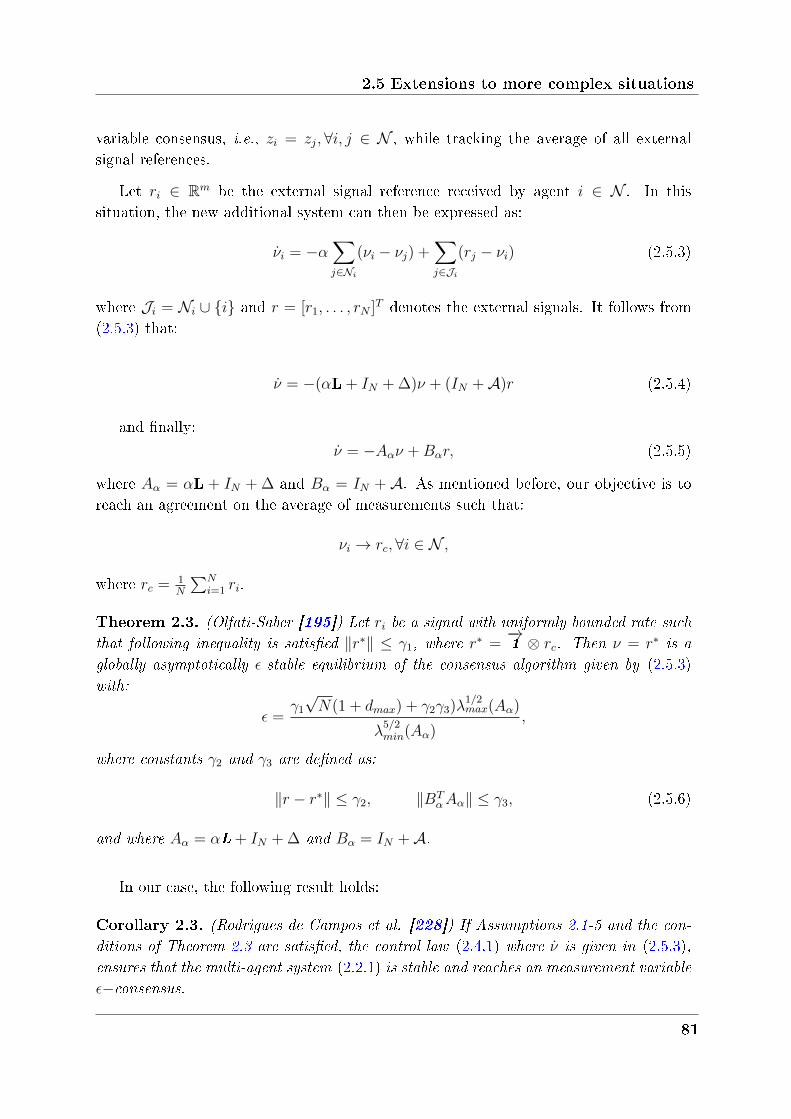
2.5 Extensions to more complex situations
variable consensus, i.e., 𝑧𝑖 = 𝑧𝑗,∀𝑖, 𝑗 ∈ 𝒩 , while tracking the average of all externalsignal references.
Let 𝑟𝑖 ∈ R𝑚 be the external signal reference received by agent 𝑖 ∈ 𝒩 . In thissituation, the new additional system can then be expressed as:
𝑖 = −𝛼∑𝑗∈𝒩𝑖
(𝜈𝑖 − 𝜈𝑗) +∑𝑗∈𝒥𝑖
(𝑟𝑗 − 𝜈𝑖) (2.5.3)
where 𝒥𝑖 = 𝒩𝑖 ∪ 𝑖 and 𝑟 = [𝑟1, . . . , 𝑟𝑁 ]𝑇 denotes the external signals. It follows from(2.5.3) that:
= −(𝛼L + 𝐼𝑁 + ∆)𝜈 + (𝐼𝑁 + 𝒜)𝑟 (2.5.4)
and nally:
= −𝐴𝛼𝜈 +𝐵𝛼𝑟, (2.5.5)
where 𝐴𝛼 = 𝛼L + 𝐼𝑁 + ∆ and 𝐵𝛼 = 𝐼𝑁 + 𝒜. As mentioned before, our objective is toreach an agreement on the average of measurements such that:
𝜈𝑖 → 𝑟𝑐,∀𝑖 ∈ 𝒩 ,
where 𝑟𝑐 = 1𝑁
∑𝑁𝑖=1 𝑟𝑖.
Theorem 2.3. (Olfati-Saber [195]) Let 𝑟𝑖 be a signal with uniformly bounded rate such
that following inequality is satisfied ‖𝑟*‖ ≤ 𝛾1, where 𝑟* =
−→1 ⊗ 𝑟𝑐. Then 𝜈 = 𝑟* is a
globally asymptotically 𝜖-stable equilibrium of the consensus algorithm given by (2.5.3)with:
𝜖 =𝛾1√𝑁(1 + 𝑑𝑚𝑎𝑥) + 𝛾2𝛾3)𝜆
1/2𝑚𝑎𝑥(𝐴𝛼)
𝜆5/2𝑚𝑖𝑛(𝐴𝛼)
,
where constants 𝛾2 and 𝛾3 are defined as:
‖𝑟 − 𝑟*‖ ≤ 𝛾2, ‖𝐵𝑇𝛼𝐴𝛼‖ ≤ 𝛾3, (2.5.6)
and where 𝐴𝛼 = 𝛼L + 𝐼𝑁 + ∆ and 𝐵𝛼 = 𝐼𝑁 + 𝒜.
In our case, the following result holds:
Corollary 2.3. (Rodrigues de Campos et al. [228]) If Assumptions 2.1-5 and the con-
ditions of Theorem 2.3 are satisfied, the control law (2.4.1) where is given in (2.5.3),ensures that the multi-agent system (2.2.1) is stable and reaches an measurement variable
𝜖−consensus.
81
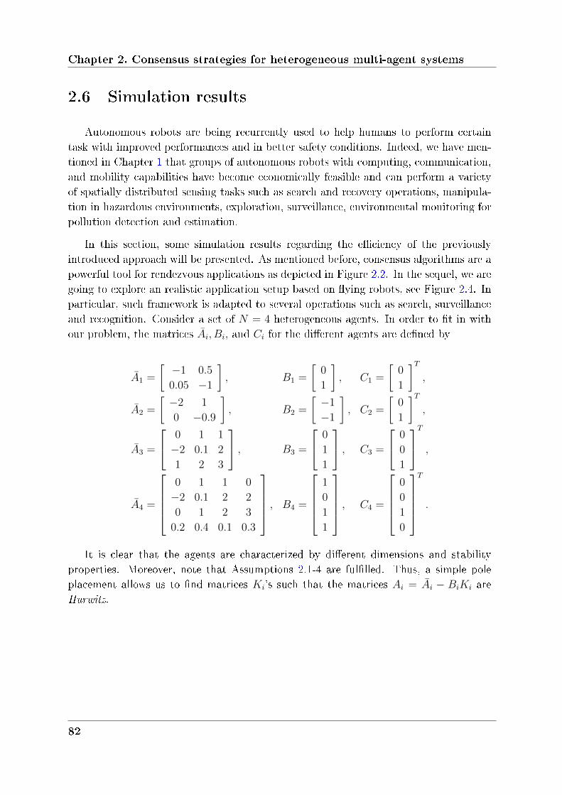
Chapter 2. Consensus strategies for heterogeneous multi-agent systems
2.6 Simulation results
Autonomous robots are being recurrently used to help humans to perform certaintask with improved performances and in better safety conditions. Indeed, we have men-tioned in Chapter 1 that groups of autonomous robots with computing, communication,and mobility capabilities have become economically feasible and can perform a varietyof spatially distributed sensing tasks such as search and recovery operations, manipula-tion in hazardous environments, exploration, surveillance, environmental monitoring forpollution detection and estimation.
In this section, some simulation results regarding the eciency of the previouslyintroduced approach will be presented. As mentioned before, consensus algorithms are apowerful tool for rendezvous applications as depicted in Figure 2.2. In the sequel, we aregoing to explore an realistic application setup based on ying robots, see Figure 2.4. Inparticular, such framework is adapted to several operations such as search, surveillanceand recognition. Consider a set of 𝑁 = 4 heterogeneous agents. In order to t in withour problem, the matrices 𝐴𝑖, 𝐵𝑖, and 𝐶𝑖 for the dierent agents are dened by
𝐴1 =
[ −1 0.5
0.05 −1
], 𝐵1 =
[0
1
], 𝐶1 =
[0
1
]𝑇,
𝐴2 =
[ −2 1
0 −0.9
], 𝐵2 =
[ −1
−1
], 𝐶2 =
[0
1
]𝑇,
𝐴3 =
⎡⎣ 0 1 1
−2 0.1 2
1 2 3
⎤⎦ , 𝐵3 =
⎡⎣ 0
1
1
⎤⎦ , 𝐶3 =
⎡⎣ 0
0
1
⎤⎦𝑇 ,
𝐴4 =
⎡⎢⎢⎢⎣0 1 1 0
−2 0.1 2 2
0 1 2 3
0.2 0.4 0.1 0.3
⎤⎥⎥⎥⎦ , 𝐵4 =
⎡⎢⎢⎢⎣1
0
1
1
⎤⎥⎥⎥⎦ , 𝐶4 =
⎡⎢⎢⎢⎣0
0
1
0
⎤⎥⎥⎥⎦𝑇
.
It is clear that the agents are characterized by dierent dimensions and stabilityproperties. Moreover, note that Assumptions 2.1-4 are fullled. Thus, a simple poleplacement allows us to nd matrices 𝐾𝑖's such that the matrices 𝐴𝑖 = 𝐴𝑖 − 𝐵𝑖𝐾𝑖 areHurwitz.
82
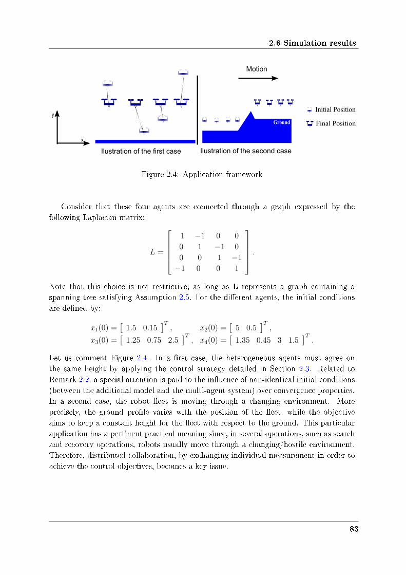
2.6 Simulation results
y
Ilustration of the first case Ilustration of the second case
Ground
Initial Position
Final Position
x
Motion
Figure 2.4: Application framework
Consider that these four agents are connected through a graph expressed by thefollowing Laplacian matrix:
𝐿 =
⎡⎢⎢⎢⎣1 −1 0 0
0 1 −1 0
0 0 1 −1
−1 0 0 1
⎤⎥⎥⎥⎦ .Note that this choice is not restrictive, as long as L represents a graph containing aspanning tree satisfying Assumption 2.5. For the dierent agents, the initial conditionsare dened by:
𝑥1(0) =[
1.5 0.15]𝑇, 𝑥2(0) =
[5 0.5
]𝑇,
𝑥3(0) =[
1.25 0.75 2.5]𝑇, 𝑥4(0) =
[1.35 0.45 3 1.5
]𝑇.
Let us comment Figure 2.4. In a rst case, the heterogeneous agents must agree onthe same height by applying the control strategy detailed in Section 2.3. Related toRemark 2.2, a special attention is paid to the inuence of non-identical initial conditions(between the additional model and the multi-agent system) over convergence properties.In a second case, the robot eet is moving through a changing environment. Moreprecisely, the ground prole varies with the position of the eet, while the objectiveaims to keep a constant height for the eet with respect to the ground. This particularapplication has a pertinent practical meaning since, in several operations, such as searchand recovery operations, robots usually move through a changing/hostile environment.Therefore, distributed collaboration, by exchanging individual measurement in order toachieve the control objectives, becomes a key issue.
83
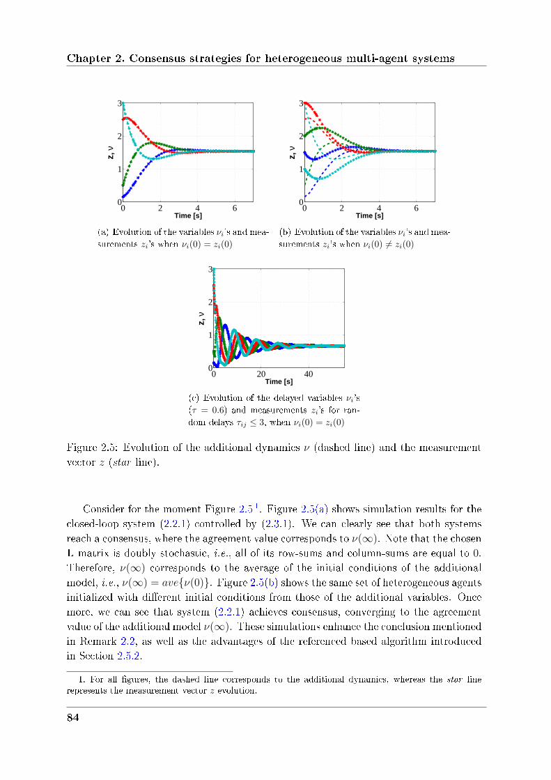
Chapter 2. Consensus strategies for heterogeneous multi-agent systems
0 2 4 60
1
2
3z,
ν
Time [s]
(a) Evolution of the variables 𝜈𝑖’s and mea-
surements 𝑧𝑖’s when 𝜈𝑖(0) = 𝑧𝑖(0)
0 2 4 60
1
2
3
z, ν
Time [s]
(b) Evolution of the variables 𝜈𝑖’s and mea-
surements 𝑧𝑖’s when 𝜈𝑖(0) = 𝑧𝑖(0)
0 20 400
1
2
3
z, ν
Time [s]
(c) Evolution of the delayed variables 𝜈𝑖’s
(𝜏 = 0.6) and measurements 𝑧𝑖’s for ran-
dom delays 𝜏𝑖𝑗 ≤ 3, when 𝜈𝑖(0) = 𝑧𝑖(0)
Figure 2.5: Evolution of the additional dynamics 𝜈 (dashed line) and the measurementvector 𝑧 (star line).
Consider for the moment Figure 2.5 1. Figure 2.5(a) shows simulation results for theclosed-loop system (2.2.1) controlled by (2.3.1). We can clearly see that both systemsreach a consensus, where the agreement value corresponds to 𝜈(∞). Note that the chosenL matrix is doubly stochastic, i.e., all of its row-sums and column-sums are equal to 0.Therefore, 𝜈(∞) corresponds to the average of the initial conditions of the additionalmodel, i.e., 𝜈(∞) = 𝑎𝑣𝑒𝜈(0). Figure 2.5(b) shows the same set of heterogeneous agentsinitialized with dierent initial conditions from those of the additional variables. Oncemore, we can see that system (2.2.1) achieves consensus, converging to the agreementvalue of the additional model 𝜈(∞). These simulations enhance the conclusion mentionedin Remark 2.2, as well as the advantages of the referenced based algorithm introducedin Section 2.5.2.
1. For all figures, the dashed line corresponds to the additional dynamics, whereas the star linerepresents the measurement vector 𝑧 evolution.
84
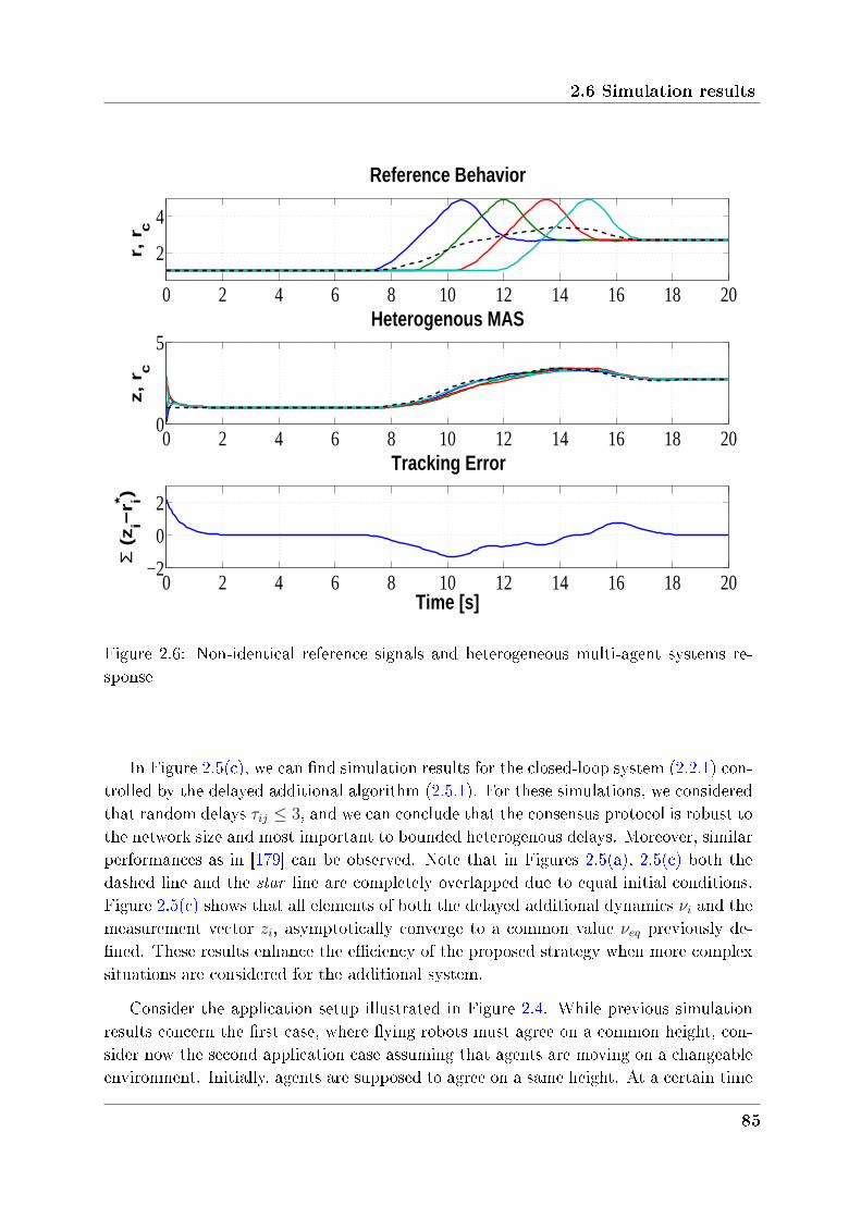
2.6 Simulation results
0 2 4 6 8 10 12 14 16 18 20
2
4
r, r
c
Reference Behavior
0 2 4 6 8 10 12 14 16 18 200
5Heterogenous MAS
z, r c
0 2 4 6 8 10 12 14 16 18 20−2
0
2
Tracking Error
Time [s]
Σ (
zi−
r i* )
Figure 2.6: Non-identical reference signals and heterogeneous multi-agent systems re-sponse
In Figure 2.5(c), we can nd simulation results for the closed-loop system (2.2.1) con-trolled by the delayed additional algorithm (2.5.1). For these simulations, we consideredthat random delays 𝜏𝑖𝑗 ≤ 3, and we can conclude that the consensus protocol is robust tothe network size and most important to bounded heterogenous delays. Moreover, similarperformances as in [179] can be observed. Note that in Figures 2.5(a), 2.5(c) both thedashed line and the star line are completely overlapped due to equal initial conditions.Figure 2.5(c) shows that all elements of both the delayed additional dynamics 𝜈𝑖 and themeasurement vector 𝑧𝑖, asymptotically converge to a common value 𝜈𝑒𝑞 previously de-ned. These results enhance the eciency of the proposed strategy when more complexsituations are considered for the additional system.
Consider the application setup illustrated in Figure 2.4. While previous simulationresults concern the rst case, where ying robots must agree on a common height, con-sider now the second application case assuming that agents are moving on a changeableenvironment. Initially, agents are supposed to agree on a same height. At a certain time
85
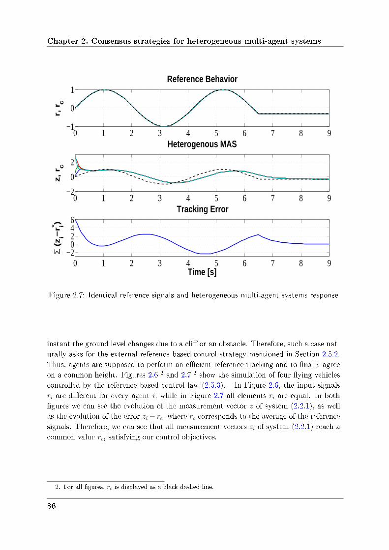
Chapter 2. Consensus strategies for heterogeneous multi-agent systems
0 1 2 3 4 5 6 7 8 9−1
0
1
r, r
c
Reference Behavior
0 1 2 3 4 5 6 7 8 9−2
0
2
Heterogenous MAS
z, r c
0 1 2 3 4 5 6 7 8 9−2
0246
Tracking Error
Time [s]
Σ (
zi−
r i* )
Figure 2.7: Identical reference signals and heterogeneous multi-agent systems response
instant the ground level changes due to a cli or an obstacle. Therefore, such a case nat-urally asks for the external reference based control strategy mentioned in Section 2.5.2.Thus, agents are supposed to perform an ecient reference tracking and to nally agreeon a common height. Figures 2.6 2 and 2.7 2 show the simulation of four ying vehiclescontrolled by the reference based control law (2.5.3). In Figure 2.6, the input signals𝑟𝑖 are dierent for every agent 𝑖, while in Figure 2.7 all elements 𝑟𝑖 are equal. In bothgures we can see the evolution of the measurement vector 𝑧 of system (2.2.1), as wellas the evolution of the error 𝑧𝑖− 𝑟𝑐, where 𝑟𝑐 corresponds to the average of the referencesignals. Therefore, we can see that all measurement vectors 𝑧𝑖 of system (2.2.1) reach acommon value 𝑟𝑐, satisfying our control objectives.
2. For all figures, 𝑟𝑐 is displayed as a black dashed line.
86
2.7 Conclusions
2.7 Conclusions
In this chapter, a novel approach under which heterogeneous multi-agent systemsreach measurement variable consensus has been presented, designed and analyzed. More-over, Section 2.6 show the eciency of our approach. We have shown that by using simpleadditional dynamics, the control of a high order heterogeneous multi-agent system notonly becomes possible, but can be done with low constraints on system (2.2.1) and withlow computational loads. The major advantage of the proposed algorithm remains inthe separation of the stability analysis of each subsystem and the distributed control al-gorithm. As a result, we have also shown that dierent additional dynamics can be used,such as delayed Simple Integrator (SI) consensus and distributed consensus lter algo-rithms. This approach, when compared with the available results on literature, appearsto have good performances, since other solutions oer some drawbacks as calculationcomplexity or restrictive assumptions.
The use of networks certainly oers several advantages, but not without drawbacks.In fact, the use of a shared network introduces new challenges, such as delays overcommunications, delays, data loss, or even communication blackout, see Chapter 1 andthe references therein. Consequently, the Laplacian and its spectral properties [106, 168]play a crucial role in convergence analysis of consensus and alignment algorithms. Inseveral multi-agent control problems, the convergence properties and speed of the systemdepend on the algebraic connectivity of the graph. Therefore, a special attention in paidin the sequel to the second smallest eigenvalue of graph's Laplacian, also called algebraicconnectivity and that quanties the speed of convergence of consensus algorithms. Someinteresting and challenging questions recently raised by our community are still to bepartially answered: (i) Is it possible to increase the convergence speed of a consensusalgorithm? and (ii) If yes, how?
An approach able to answer these questions will be presented in the next chapter.
87
Chapter 2. Consensus strategies for heterogeneous multi-agent systems
88
Chapter 3
Improved stability of consensus
algorithms
Contents
3.1 Context . . . . . . . . . . . . . . . . . . . . . . . . . . . . . . . 90
3.2 Simple integrator dynamics . . . . . . . . . . . . . . . . . . . 91
3.2.1 Problem statement and preliminaries . . . . . . . . . . . . . . . 91
3.2.2 Partial memory . . . . . . . . . . . . . . . . . . . . . . . . . . . 92
3.2.3 Global memory . . . . . . . . . . . . . . . . . . . . . . . . . . . 99
3.3 Double integrator dynamics . . . . . . . . . . . . . . . . . . . 102
3.3.1 Problem statement and preliminaries . . . . . . . . . . . . . . . 102
3.3.2 Controller design . . . . . . . . . . . . . . . . . . . . . . . . . . 104
3.3.3 Definition of an appropriate model . . . . . . . . . . . . . . . . 105
3.3.4 Stability analysis . . . . . . . . . . . . . . . . . . . . . . . . . . 106
3.4 Simulation results . . . . . . . . . . . . . . . . . . . . . . . . . 108
3.5 Conclusions . . . . . . . . . . . . . . . . . . . . . . . . . . . . . 122
Chapter 3. Improved stability of consensus algorithms
3.1 Context
As for the previous chapter, the sequel focuses on consensus algorithms as one of theuseful tools available for multi-agent systems agreement and in particular to rendezvousprotocols, see Figure 2.1. While in the previous chapter we focus on the design of eectiveconsensus algorithms for heterogeneous MAS, in this chapter a special attention is paid toconsensus algorithm's convergence rate. More precisely, we will try to improve traditionalconvergence properties using memory based approaches.
In several multi-agent control problems, the convergence properties and speed of thesystem depend on the algebraic connectivity of the graph. The algebraic connectivityis an important network property for all the previous systems to reach convergence andit characterizes the convergence rate. More precisely, the algebraic connectivity is equalto the second smallest eigenvalue of L. Connectivity control methods establish agentmotions that preserve or maximize some network connectivity property. An optimizationmethod of the topology-respecting weight matrix summarizing the updates at each nodeis presented in [112, 304] and the 𝑘-connectivity matrix of the graph is computed in acentralized fashion in [313]. Several distributed methods compute spanning subgraphs[314], specic Laplacian eigenvectors [212] or moments (mean, variance, skewness andkurtosis) of the Laplacian eigenvalue spectrum [210]. Some other works also maximizethe algebraic connectivity through motion control without actually computing it, see,e.g., [255]. Moreover, a distributed algebraic connectivity estimation method is proposedin [4]. More precisely, authors discuss a particular event-triggered consensus scenario andshow that the availability of an estimate of the algebraic connectivity could be used foradapting the behavior of the average consensus algorithm.
Accelerating the convergence of distributed consensus algorithms have been also stud-ied in literature by incorporating memory into the control laws. This chapter focusesin this specic approach. Even if for most applications delays lead to a reduction ofperformance and instability, in some cases the introduction of a delay in the control loopcan help to stabilize a system. This has been studied in [110, 252]. More precisely, in[252] authors added a state sampled component to the control law, what can be seenas an articial way to manipulate L's eigenvalues, by getting them further onto the leftpart of the complex plan. Considering Denition 1.7, this inherently means that thespeed of convergence will change. An approach based on [252] will be proposed in thesequel aiming to maximize the speed of convergence. It is worth mentioning that theseworks are related with the International Research Group Groupement International deRecherche (GDRI) DelSys, supported by the Centre National de la Recherche Scien-tique (CNRS). In the sequel, we consider both simple and double integrator dynamicsand the communication graphs are supposed to be directed and undirected.
90
3.2 Simple integrator dynamics
3.2 Simple integrator dynamics
3.2.1 Problem statement and preliminaries
In the scope of multi-robots systems, we are particulary motivated by motion controlin a cartesian plane. Consequently, the position of each agent 𝑖 is denoted
𝑞𝑖 = [𝑥𝑖, 𝑦𝑖]𝑇 ∈ R2,
where 𝑥𝑖 and 𝑦𝑖 represent the dynamics of 𝑞𝑖 on the x-axis and y-axis, respectively.However, for the sake of notation's clearness and without loss of generality, in this chapterwe consider only the dynamics of 𝑥𝑖.
Simple integrator dynamics are a particular case of the linear MAS widely used inliterature [13, 176, 194, 251]. As mentioned before, we are interested in motion controlof robot swarms, and in particular in rendezvous applications, see [62]. The desiredbehavior is depicted in Figure 3.1.
Consider the classical SI consensus algorithm given by:
𝑖(𝑡) = 𝑢𝑖(𝑡)
𝑢𝑖(𝑡) =∑
𝑗∈𝒩𝑖𝑎𝑖𝑗(𝑥𝑗(𝑡) − 𝑥𝑖(𝑡))
𝑖 ∈ 1, . . . , 𝑁, (3.2.1)
where 𝑥𝑖 represents agent 𝑖 variables. Introducing the vector 𝑥(𝑡) = [𝑥1(𝑡), .., 𝑥𝑁(𝑡)]𝑇
containing the state of all agents, we then derive:
(𝑡) = −L𝑥(𝑡) , (3.2.2)
where L is the Laplacian matrix. This algorithm is distributed in the sense that eachagent has only access to information from its neighbors. Assume that there exist aconstant and positive scalar 𝜇 such that:∑
𝑗∈𝒩𝑖
𝑎𝑖𝑗 = 𝜇, 𝑖 ∈ 1, . . . , 𝑁.
Since for achieving consensus some assumptions on the communication graph mustbe satised, the following assumptions hold.
Assumption 3.1. (Graph’s Variance): For any considered graph 𝒢, we assume thatthe communication graph expressing neighborhood relations between agents is constant,
and therefore the corresponding Laplacian matrix L is time-invariant.
Other communication properties such as the presence of noise, packet loss and timedelays will not be considered.
91
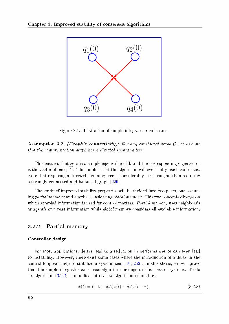
Chapter 3. Improved stability of consensus algorithms
q1(0) q2(0)
q3(0) q4(0)
Figure 3.1: Illustration of simple integrator rendezvous
Assumption 3.2. (Graph’s connectivity): For any considered graph 𝒢, we assume
that the communication graph has a directed spanning tree.
This ensures that zero is a simple eigenvalue of L and the corresponding eigenvectoris the vector of ones,
−→1 . This implies that the algorithm will eventually reach consensus.
Note that requiring a directed spanning tree is considerably less stringent than requiringa strongly connected and balanced graph [220].
The study of improved stability properties will be divided into two parts, one assum-ing partial memory and another considering global memory. This two concepts diverge onwhich sampled information is used for control matters. Partial memory uses neighbors'sor agent's own past information while global memory considers all available information.
3.2.2 Partial memory
Controller design
For most applications, delays lead to a reduction in performances or can even leadto instability. However, there exist some cases where the introduction of a delay in thecontrol loop can help to stabilize a system, see [110, 252]. In this thesis, we will provethat the simple integrator consensus algorithm belongs to this class of systems. To doso, algorithm (3.2.2) is modied into a new algorithm dened by:
(𝑡) = (−L− 𝛿𝒜)𝑥(𝑡) + 𝛿𝒜𝑥(𝑡− 𝜏), (3.2.3)
92
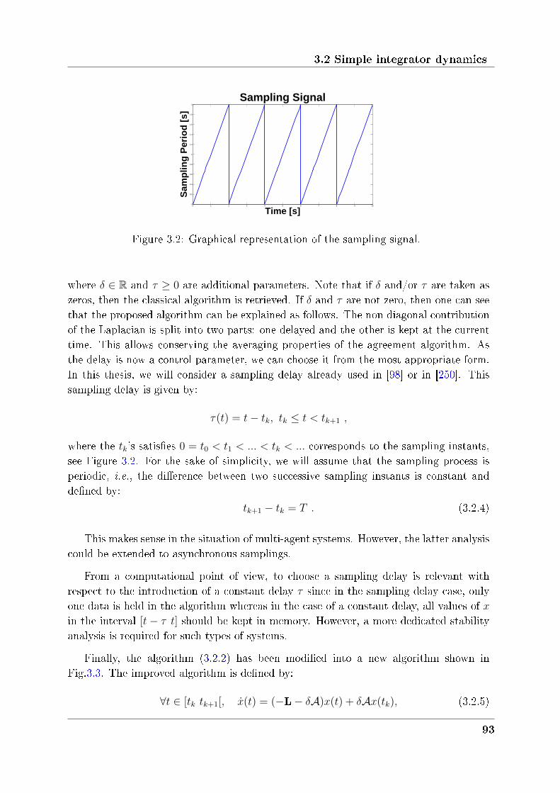
3.2 Simple integrator dynamics
0 1 2 3 4 5 6 7 8 9 100
0.2
0.4
0.6
0.8
1
1.2
1.4
1.6
1.8
2
Time [s]
Sam
plin
g P
erio
d [
s]
Sampling Signal
Figure 3.2: Graphical representation of the sampling signal.
where 𝛿 ∈ R and 𝜏 ≥ 0 are additional parameters. Note that if 𝛿 and/or 𝜏 are taken aszeros, then the classical algorithm is retrieved. If 𝛿 and 𝜏 are not zero, then one can seethat the proposed algorithm can be explained as follows. The non diagonal contributionof the Laplacian is split into two parts: one delayed and the other is kept at the currenttime. This allows conserving the averaging properties of the agreement algorithm. Asthe delay is now a control parameter, we can choose it from the most appropriate form.In this thesis, we will consider a sampling delay already used in [98] or in [250]. Thissampling delay is given by:
𝜏(𝑡) = 𝑡− 𝑡𝑘, 𝑡𝑘 ≤ 𝑡 < 𝑡𝑘+1 ,
where the 𝑡𝑘's satises 0 = 𝑡0 < 𝑡1 < ... < 𝑡𝑘 < ... corresponds to the sampling instants,see Figure 3.2. For the sake of simplicity, we will assume that the sampling process isperiodic, i.e., the dierence between two successive sampling instants is constant anddened by:
𝑡𝑘+1 − 𝑡𝑘 = 𝑇 . (3.2.4)
This makes sense in the situation of multi-agent systems. However, the latter analysiscould be extended to asynchronous samplings.
From a computational point of view, to choose a sampling delay is relevant withrespect to the introduction of a constant delay 𝜏 since in the sampling delay case, onlyone data is held in the algorithm whereas in the case of a constant delay, all values of 𝑥in the interval [𝑡− 𝜏 𝑡] should be kept in memory. However, a more dedicated stabilityanalysis is required for such types of systems.
Finally, the algorithm (3.2.2) has been modied into a new algorithm shown inFig.3.3. The improved algorithm is dened by:
∀𝑡 ∈ [𝑡𝑘 𝑡𝑘+1[, (𝑡) = (−L− 𝛿𝒜)𝑥(𝑡) + 𝛿𝒜𝑥(𝑡𝑘), (3.2.5)
93
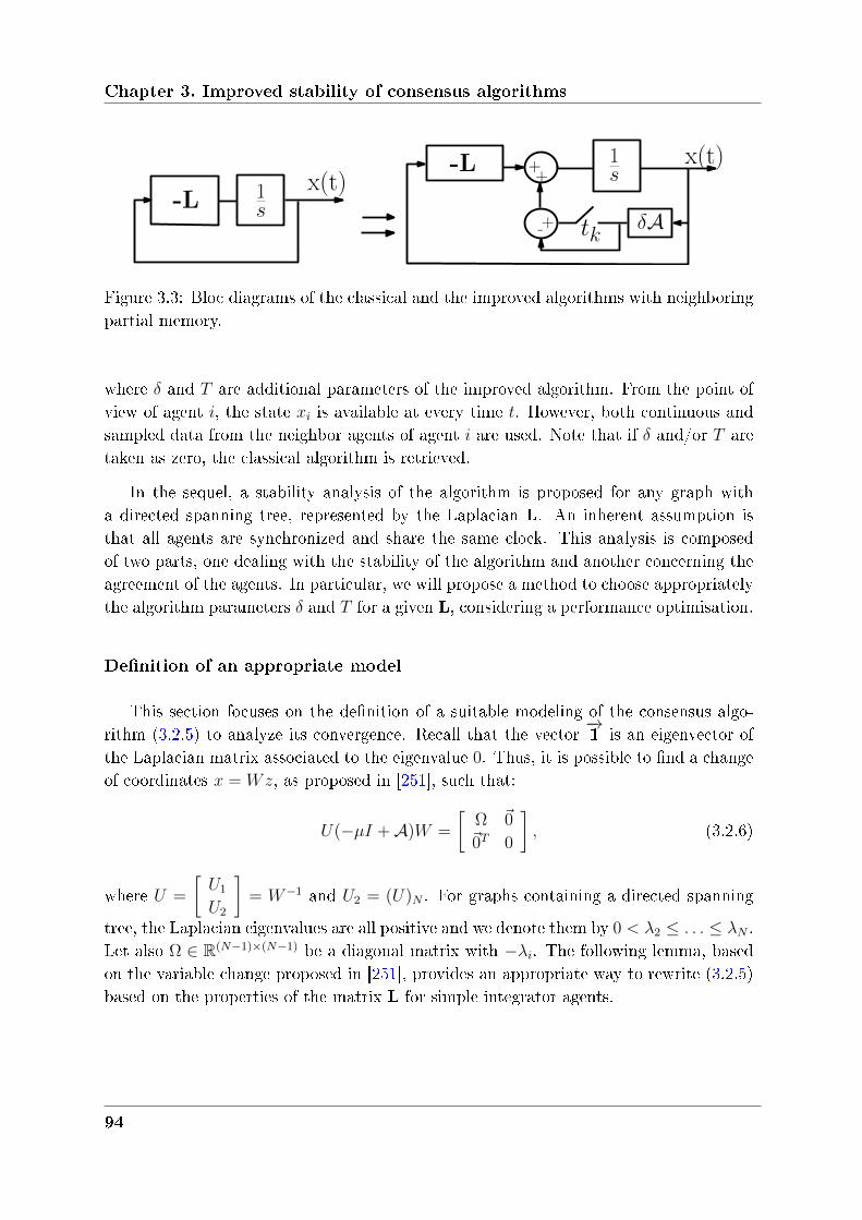
Chapter 3. Improved stability of consensus algorithms
-L x(t)
δA
+x(t)
tk-+
+1s
1s-L
Figure 3.3: Bloc diagrams of the classical and the improved algorithms with neighboringpartial memory.
where 𝛿 and 𝑇 are additional parameters of the improved algorithm. From the point ofview of agent 𝑖, the state 𝑥𝑖 is available at every time 𝑡. However, both continuous andsampled data from the neighbor agents of agent 𝑖 are used. Note that if 𝛿 and/or 𝑇 aretaken as zero, the classical algorithm is retrieved.
In the sequel, a stability analysis of the algorithm is proposed for any graph witha directed spanning tree, represented by the Laplacian L. An inherent assumption isthat all agents are synchronized and share the same clock. This analysis is composedof two parts, one dealing with the stability of the algorithm and another concerning theagreement of the agents. In particular, we will propose a method to choose appropriatelythe algorithm parameters 𝛿 and 𝑇 for a given L, considering a performance optimisation.
Definition of an appropriate model
This section focuses on the denition of a suitable modeling of the consensus algo-rithm (3.2.5) to analyze its convergence. Recall that the vector
−→1 is an eigenvector of
the Laplacian matrix associated to the eigenvalue 0. Thus, it is possible to nd a changeof coordinates 𝑥 = 𝑊𝑧, as proposed in [251], such that:
𝑈(−𝜇𝐼 + 𝒜)𝑊 =
[Ω 0
0𝑇 0
], (3.2.6)
where 𝑈 =
[𝑈1
𝑈2
]= 𝑊−1 and 𝑈2 = (𝑈)𝑁 . For graphs containing a directed spanning
tree, the Laplacian eigenvalues are all positive and we denote them by 0 < 𝜆2 ≤ . . . ≤ 𝜆𝑁 .Let also Ω ∈ R(𝑁−1)×(𝑁−1) be a diagonal matrix with −𝜆𝑖. The following lemma, basedon the variable change proposed in [251], provides an appropriate way to rewrite (3.2.5)based on the properties of the matrix L for simple integrator agents.
94
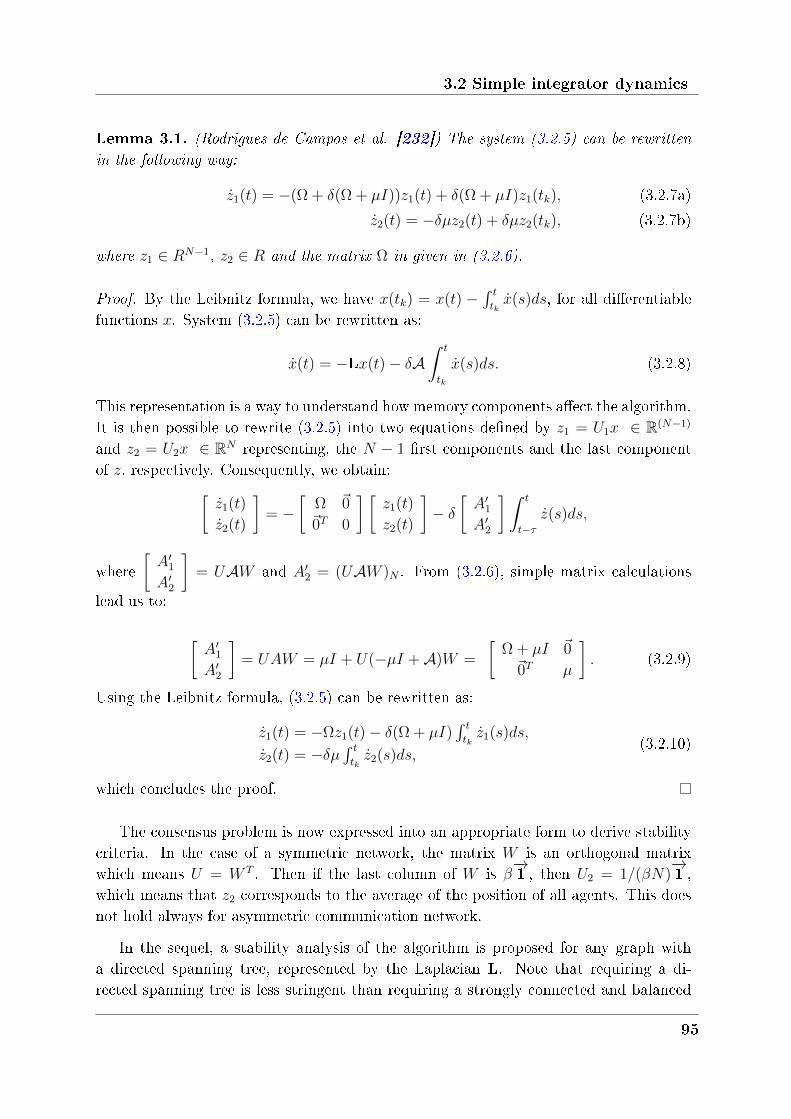
3.2 Simple integrator dynamics
Lemma 3.1. (Rodrigues de Campos et al. [232]) The system (3.2.5) can be rewritten
in the following way:
1(𝑡) = −(Ω + 𝛿(Ω + 𝜇𝐼))𝑧1(𝑡) + 𝛿(Ω + 𝜇𝐼)𝑧1(𝑡𝑘), (3.2.7a)
2(𝑡) = −𝛿𝜇𝑧2(𝑡) + 𝛿𝜇𝑧2(𝑡𝑘), (3.2.7b)
where 𝑧1 ∈ 𝑅𝑁−1, 𝑧2 ∈ 𝑅 and the matrix Ω in given in (3.2.6).
Proof. By the Leibnitz formula, we have 𝑥(𝑡𝑘) = 𝑥(𝑡) −∫ 𝑡𝑡𝑘(𝑠)𝑑𝑠, for all dierentiable
functions 𝑥. System (3.2.5) can be rewritten as:
(𝑡) = −L𝑥(𝑡) − 𝛿𝒜∫ 𝑡
𝑡𝑘
(𝑠)𝑑𝑠. (3.2.8)
This representation is a way to understand how memory components aect the algorithm.It is then possible to rewrite (3.2.5) into two equations dened by 𝑧1 = 𝑈1𝑥 ∈ R(𝑁−1)
and 𝑧2 = 𝑈2𝑥 ∈ R𝑁 representing, the 𝑁 − 1 rst components and the last componentof 𝑧, respectively. Consequently, we obtain:[
1(𝑡)
2(𝑡)
]= −
[Ω 0
0𝑇 0
] [𝑧1(𝑡)
𝑧2(𝑡)
]− 𝛿
[𝐴′
1
𝐴′2
] ∫ 𝑡
𝑡−𝜏(𝑠)𝑑𝑠,
where
[𝐴′
1
𝐴′2
]= 𝑈𝒜𝑊 and 𝐴′
2 = (𝑈𝒜𝑊 )𝑁 . From (3.2.6), simple matrix calculations
lead us to:
[𝐴′
1
𝐴′2
]= 𝑈𝐴𝑊 = 𝜇𝐼 + 𝑈(−𝜇𝐼 + 𝒜)𝑊 =
[Ω + 𝜇𝐼 0
0𝑇 𝜇
]. (3.2.9)
Using the Leibnitz formula, (3.2.5) can be rewritten as:
1(𝑡) = −Ω𝑧1(𝑡) − 𝛿(Ω + 𝜇𝐼)∫ 𝑡𝑡𝑘1(𝑠)𝑑𝑠,
2(𝑡) = −𝛿𝜇∫ 𝑡𝑡𝑘2(𝑠)𝑑𝑠,
(3.2.10)
which concludes the proof.
The consensus problem is now expressed into an appropriate form to derive stabilitycriteria. In the case of a symmetric network, the matrix 𝑊 is an orthogonal matrixwhich means 𝑈 = 𝑊 𝑇 . Then if the last column of 𝑊 is 𝛽
−→1 , then 𝑈2 = 1/(𝛽𝑁)
−→1 ,
which means that 𝑧2 corresponds to the average of the position of all agents. This doesnot hold always for asymmetric communication network.
In the sequel, a stability analysis of the algorithm is proposed for any graph witha directed spanning tree, represented by the Laplacian L. Note that requiring a di-rected spanning tree is less stringent than requiring a strongly connected and balanced
95
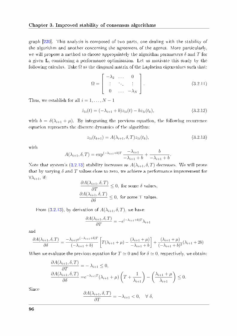
Chapter 3. Improved stability of consensus algorithms
graph [220]. This analysis is composed of two parts, one dealing with the stability ofthe algorithm and another concerning the agreement of the agents. More particularly,we will propose a method to choose appropriately the algorithm parameters 𝛿 and 𝑇 fora given L, considering a performance optimisation. Let us motivate this study by thefollowing calculus. Take Ω as the diagonal matrix of the Laplacian eigenvalues such that:
Ω =
⎡⎢⎣ −𝜆2 . . . 0...
. . ....
0 . . . −𝜆𝑁
⎤⎥⎦ . (3.2.11)
Thus, we establish for all 𝑖 = 1, . . . , 𝑁 − 1
1𝑖(𝑡) = (−𝜆𝑖+1 + 𝑏)𝑧1𝑖(𝑡) − 𝑏𝑧1𝑖(𝑡𝑘), (3.2.12)
with 𝑏 = 𝛿(𝜆𝑖+1 + 𝜇). By integrating the previous equation, the following recurrenceequation represents the discrete dynamics of the algorithm:
𝑧1𝑖(𝑡𝑘+1) = 𝐴(𝜆𝑖+1, 𝛿, 𝑇 )𝑧1𝑖(𝑡𝑘), (3.2.13)
with
𝐴(𝜆𝑖+1, 𝛿, 𝑇 ) = exp(−𝜆𝑖+1+𝑏)𝑇−𝜆𝑖+1
−𝜆𝑖+1 + 𝑏+
𝑏
−𝜆𝑖+1 + 𝑏.
Note that system's (3.2.13) stability increases as 𝐴(𝜆𝑖+1, 𝛿, 𝑇 ) decreases. We will provethat by varying 𝛿 and 𝑇 values close to zero, we achieve a performance improvement for∀𝜆𝑖+1, if:
𝜕𝐴(𝜆𝑖+1, 𝛿, 𝑇 )
𝜕𝑇≤ 0, for some 𝛿 values,
𝜕𝐴(𝜆𝑖+1, 𝛿, 𝑇 )
𝜕𝛿≤ 0, for some T values.
From (3.2.13), by derivation of 𝐴(𝜆𝑖+1, 𝛿, 𝑇 ), we have:
𝜕𝐴(𝜆𝑖+1, 𝛿, 𝑇 )
𝜕𝑇= −𝑒(−𝜆𝑖+1+𝑏)𝑇𝜆𝑖+1
and
𝜕𝐴(𝜆𝑖+1, 𝛿, 𝑇 )
𝜕𝛿=
−𝜆𝑖+1𝑒(−𝜆𝑖+1+𝑏)𝑇
(−𝜆𝑖+1 + 𝑏)
[𝑇 (𝜆𝑖+1 + 𝜇)− (𝜆𝑖+1 + 𝜇)
−𝜆𝑖+1 + 𝑏
]+
(𝜆𝑖+1 + 𝜇)
(−𝜆𝑖+1 + 𝑏)2(𝜆𝑖+1 + 2𝑏)
When we evaluate the previous equation for 𝑇 ≃ 0 and for 𝛿 ≃ 0, respectively, we obtain:
𝜕𝐴(𝜆𝑖+1, 𝛿, 𝑇 )
𝜕𝑇= − 𝜆𝑖+1 ≤ 0,
𝜕𝐴(𝜆𝑖+1, 𝛿, 𝑇 )
𝜕𝛿=𝑒−𝜆𝑖+1𝑇 (𝜆𝑖+1 + 𝜇)
(𝑇 +
1
𝜆𝑖+1
)−(𝜆𝑖+1 + 𝜇
𝜆𝑖+1
)≤ 0.
Since𝜕𝐴(𝜆𝑖+1, 𝛿, 𝑇 )
𝜕𝑇= −𝜆𝑖+1 < 0, ∀ 𝛿,
96
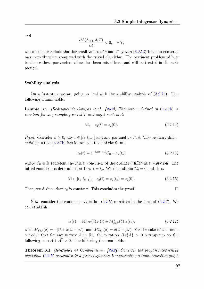
3.2 Simple integrator dynamics
and𝜕𝐴(𝜆𝑖+1, 𝛿, 𝑇 )
𝜕𝛿< 0, ∀ 𝑇,
we can then conclude that for small values of 𝛿 and 𝑇 system (3.2.13) tends to convergemore rapidly when compared with the trivial algorithm. The pertinent problem of howto choose these parameters values has been raised here, and will be treated in the nextsection.
Stability analysis
On a rst step, we are going to deal with the stability analysis of (3.2.7b). Thefollowing lemma holds.
Lemma 3.2. (Rodrigues de Campos et al. [232]) The system defined in (3.2.7b) is
constant for any sampling period 𝑇 and any 𝛿 such that:
∀𝑡, 𝑧2(𝑡) = 𝑧2(0). (3.2.14)
Proof. Consider 𝑘 ≥ 0, any 𝑡 ∈ [𝑡𝑘 𝑡𝑘+1[ and any parameters 𝑇 , 𝛿. The ordinary dier-ential equation (3.2.7b) has known solutions of the form:
𝑧2(𝑡) = 𝑒−𝛿𝜇(𝑡−𝑡𝑘)𝐶0 − 𝑧2(𝑡𝑘) (3.2.15)
where 𝐶0 ∈ R represent the initial condition of the ordinary dierential equation. Theinitial condition is determined at time 𝑡 = 𝑡𝑘. We then obtain 𝐶0 = 0 and thus:
∀𝑡 ∈ [𝑡𝑘 𝑡𝑘+1[, 𝑧2(𝑡) = 𝑧2(𝑡𝑘) = 𝑧2(0). (3.2.16)
Then, we deduce that 𝑧2 is constant. This concludes the proof.
Now, consider the consensus algorithm (3.2.5) rewritten in the form of (3.2.7). Wecan establish:
1(𝑡) = 𝑀𝑆𝐼𝑃 (𝛿)𝑧1(𝑡) +𝑀*𝑆𝐼𝑃 (𝛿)𝑧1(𝑡𝑘), (3.2.17)
with 𝑀𝑆𝐼𝑃 (𝛿) = −[Ω + 𝛿(Ω + 𝜇𝐼)] and 𝑀*𝑆𝐼𝑃 (𝛿) = 𝛿(Ω + 𝜇𝐼). For the sake of clearness,
consider that for any matrix 𝐴 in R𝑛, the notation 𝐻𝑒𝐴 > 0 corresponds to thefollowing sum 𝐴+ 𝐴𝑇 > 0. The following theorem holds.
Theorem 3.1. (Rodrigues de Campos et al. [232]) Consider the proposed consensus
algorithm (3.2.5) associated to a given Laplacian L representing a communication graph
97
Chapter 3. Improved stability of consensus algorithms
with a directed spanning tree, a given 𝛼 > 0, 𝛿 > 0, and 𝑇 > 0. Assume that there exist
𝑃 > 0, 𝑅 > 0, 𝑆1 and 𝑋 ∈ S𝑛, 𝑆2 ∈ R𝑛×𝑛 and 𝑁 ∈ R2𝑛×𝑛 that satisfy
Ψ1(𝑇 ) = 𝑒𝛼(𝜏)Π1 + 𝑓𝛼(𝑇, 0)Π2 + ℎ𝛼(𝑇, 0)Π3 < 0,
Ψ2(𝑇 ) =
[𝑒𝛼(𝑇 )Π1 + ℎ𝛼(𝑇, 𝑇 )Π3 𝑔𝛼(𝑇, 𝑇 )𝑁
* −𝑔𝛼(𝑇, 𝑇 )𝑅
]< 0,
(3.2.18)
whereΠ1 = 𝐻𝑒𝑀𝑇
1 𝑃𝑀0 −𝑀𝑇12(
12𝑆1𝑀12 + 𝑆2𝑀2 +𝑁𝑇 ) + 2𝛼𝑀𝑇
1 𝑃𝑀1
Π2 = 𝑀𝑇0 𝑅𝑀0 +𝐻𝑒𝑀𝑇
0 (𝑆1𝑀12 + 𝑆2𝑀2),Π3 = 𝑀𝑇
2 𝑋𝑀2,
and 𝑀0 =[𝑀𝑆𝐼𝑃 (𝛿) 𝑀*
𝑆𝐼𝑃 (𝛿)], 𝑀1 =
[𝐼 0
], 𝑀2 =
[0 𝐼
], 𝑀12 = 𝑀1−𝑀2. The
functions 𝑓𝛼, 𝑔𝛼 and ℎ𝛼 for all scalars 𝑇 and 𝜏 ∈ [0 𝑇 ] are given by:
𝑒𝛼(𝜏) = 𝑒2𝛼𝜏 ,
𝑓𝛼(𝑇, 𝜏) = (𝑒2𝛼𝑇 − 𝑒2𝛼𝜏 )/2𝛼,
𝑔𝛼(𝑇, 𝜏) =
𝑒2𝛼𝑇 (𝑒2𝛼𝜏 − 1)/2𝛼, if 𝛼 > 0
(𝑒2𝛼𝜏 − 1)/2𝛼, if 𝛼 < 0
ℎ𝛼(𝑇, 𝜏) = 1𝛼
[𝑒2𝛼𝑇−12𝛼𝑇
− 𝑒2𝛼𝜏].
Then, the consensus algorithm (3.2.5) with the parameter 𝛿 and the sampling period 𝑇
is thus 𝛼−stable. Moreover, the consensus equilibrium is given by:
𝑥(∞) = 𝑈2𝑥(0).
Proof. Consider the consensus algorithm (3.2.5). Using Lemma 3.1, the algorithm isrewritten as (3.2.7). The stability of the second equation (3.2.7b) is ensured based onthe discrete time Lyapunov theorem. Dene 𝑧1𝑘 = 𝑧1(𝑡𝑘) and introduce a quadraticLyapunov function dened by 𝑉 (𝑧1) = 𝑧1
𝑇𝑃𝑧1 for all 𝑧1 ∈ R𝑛. The objective is to ensurethat the increment ∆𝛼𝑉 (𝑧1) is negative denite [293]. A candidate for 𝜐𝛼 is dened forall 𝑡 ∈ [𝑡𝑘 𝑡𝑘+1] by:
𝜐𝛼(𝑡, 𝑧1𝑡) = 𝑓𝛼(𝑇, 𝜏)𝜁𝑇 (𝑡)[𝑆1𝜁(𝑡) + 2𝑆2𝑧1𝑘]
+𝑓𝛼(𝑇, 𝜏)∫ 𝑡𝑡𝑘𝑇1𝑘(𝜃)𝑅𝑧
𝑇1𝑘(𝜃)𝑑𝜃 + ℎ𝛼𝑧
𝑇1𝑘𝑋𝑧1𝑘,
(3.2.19)
where 𝜁(𝑡) = 𝑧1𝑡− 𝑧1𝑘, 𝑓𝛼(𝑇, 𝜏) = (𝑒2𝛼𝑇 − 𝑒2𝛼𝜏 )/2𝛼 and ℎ𝛼(𝑇, 𝜏) = 1𝛼
[𝑒2𝛼𝑇−12𝛼𝑇
− 𝑒2𝛼𝜏].
Denote 𝑊𝛼(𝑡, 𝑧1𝑡) = 𝑒2𝛼𝜏 [𝑉 (𝑧1) + 𝜐𝛼(𝑡, 𝑧1𝑡)]. Consider a positive scalar 0 < 𝜗 < 𝑇 andthe functional𝑊𝛼 at time 𝑡𝑘−𝜗 and 𝑡𝑘+𝜗. Since 𝜁(𝑡𝑘+𝜗) and 𝑓𝛼(𝑇𝑘−1, 𝑇𝑘−1−𝜗) tend to0 as 𝜗 → 0 for all 𝛼 > 0, the functional 𝜐𝛼(𝑡, 𝑧1𝑡) satises Theorem A.2 of Appendix A,extracted from [250]. Denote 𝜉(𝑠) = 𝑧1(𝑠)
𝑇 . By noting that 𝑑𝑑𝑡
(𝑒2𝛼𝜏𝑓𝛼) = −𝑒2𝛼𝜏 and𝑑𝑑𝑡
(𝑒2𝛼𝜏ℎ𝛼) = ℎ𝛼, it yields:
98
3.2 Simple integrator dynamics
𝛼(𝑡, 𝑧1𝑡) ≤ 𝜉𝑇 (𝑡)[𝑒𝛼(𝜏)[Π1 + 2𝛼𝑀𝑇1 𝑃𝑀1] + 𝑓𝛼(𝑇, 𝜏)Π2
+𝜏𝑒𝛼(𝜏)𝑁𝑅−1𝑁𝑇 + ℎ𝛼(𝑇, 𝜏)Π3]𝜉(𝑡),(3.2.20)
The previous inequality does not depend linearly on 𝜏 but on both 𝜏 and a non linearfunction of 𝜏 ,𝑒𝛼(𝑇, 𝜏) and 𝑓𝛼(𝜏). The solution proposed here is to use the convexityproperty of the exponential function ensuring that 𝑒2𝛼𝜏 ≥ 1 + 2𝛼𝜏 if 𝛼 > 0 and 𝑒−2𝛼𝜏 ≥1 + 2𝛼𝜏 if 𝛼 < 0. Consequently, for all 𝛼 = 0, 𝜏𝑒𝛼(𝜏) ≤ 𝑔𝛼(𝑇, 𝜏). Since 𝑅 and 𝑅−1 arepositive denite, we have:
𝛼(𝑡, 𝑧1𝑡) ≤ 𝜉𝑇 (𝑡)[𝑒𝛼(𝜏)Π1 + 𝑓𝛼(𝑇, 𝜏)Π2
+𝑔𝛼(𝑇, 𝜏)𝑁𝑅−1𝑁𝑇 + ℎ𝛼(𝑇, 𝜏)Π3]𝜉(𝑡),(3.2.21)
The previous inequality is linear with respect to 𝑒2𝛼𝜏 . To prove that 𝛼(𝑡, 𝑧1𝑡) is negativedenite for all 𝜏 we apply a lemma on positivity of matrix inequations taken from [182]with 𝜆(𝑡) = 𝑒−2𝛼𝜏 , which leads to:
Π1 + 𝑓𝛼(𝑇, 0)Π2 < 0,
Π1 + 𝑔𝛼(𝑇, 𝑇 )𝑁𝑅−1𝑁𝑇 < 0.
This leads to (3.2.18) using the Schur complement. Thus, the global algorithm (3.2.7)is then exponentially stable with the decay rate 𝛼. Moreover, according to Lemma 3.1,and since 𝑧1 → 0 and 𝑧2 → 𝑧2(∞), we conclude that the consensus equilibrium is:
𝑥(∞) = 𝑈2𝑥(0).
The proof is concluded by noting that 𝑧2 = 𝑈2𝑥.
Through previous calculations we presented an improved consensus algorithm basedon an appropriated sampling. We have analytically demonstrated the improved behaviorsand we derived stability conditions for the proposed problem. Throughout the nextsection, we are going to propose a dierent controller based on what we called globalmemory, i.e., where agents use all available information.
3.2.3 Global memory
Controller design
We aim now for each agent 𝑖 to keep in memory all the available information. Algo-rithm (3.2.2) is modied into a new algorithm shown in Fig. 3.4. Considering notationand notions from the previous section, the proposed algorithm can be written as:
∀𝑡 ∈ [𝑡𝑘 𝑡𝑘+1[, (𝑡) = (−L− 𝛿𝒜 + 𝜎𝐼)𝑥(𝑡) + (𝛿𝒜− 𝜎𝐼)𝑥(𝑡𝑘) . (3.2.22)
99
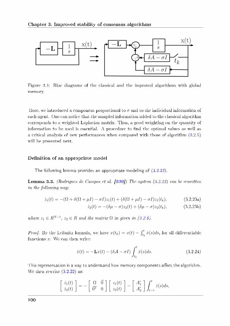
Chapter 3. Improved stability of consensus algorithms
−Lx(t)
δA− σI
+−Lx(t)
tk-+
+
δA− σI
1s1
s
Figure 3.4: Bloc diagrams of the classical and the improved algorithms with globalmemory.
Here, we introduced a component proportional to 𝜎 and to the individual information ofeach agent. One can notice that the sampled information added to the classical algorithmcorresponds to a weighted Laplacian matrix. Thus, a good weighting on the quantity ofinformation to be used is essential. A procedure to nd the optimal values as well asa critical analysis of new performances when compared with those of algorithm (3.2.5)will be presented next.
Definition of an appropriate model
The following lemma provides an appropriate modeling of (3.2.22).
Lemma 3.3. (Rodrigues de Campos et al. [230]) The system (3.2.22) can be rewritten
in the following way:
1(𝑡) = −(Ω + 𝛿(Ω + 𝜇𝐼) − 𝜎𝐼)𝑧1(𝑡) + (𝛿(Ω + 𝜇𝐼) − 𝜎𝐼)𝑧1(𝑡𝑘), (3.2.23a)
2(𝑡) = −(𝛿𝜇− 𝜎)𝑧2(𝑡) + (𝛿𝜇− 𝜎)𝑧2(𝑡𝑘), (3.2.23b)
where 𝑧1 ∈ 𝑅𝑁−1, 𝑧2 ∈ 𝑅 and the matrix Ω in given in (3.2.6).
Proof. By the Leibnitz formula, we have 𝑥(𝑡𝑘) = 𝑥(𝑡) −∫ 𝑡𝑡𝑘(𝑠)𝑑𝑠, for all dierentiable
functions 𝑥. We can then write:
(𝑡) = −L𝑥(𝑡) − (𝛿𝒜− 𝜎𝐼)
∫ 𝑡
𝑡𝑘
(𝑠)𝑑𝑠. (3.2.24)
This representation is a way to understand how memory components aect the algorithm.We then rewrite (3.2.22) as:[
1(𝑡)
2(𝑡)
]= −
[Ω 0
0𝑇 0
] [𝑧1(𝑡)
𝑧2(𝑡)
]−[𝐴′
1
𝐴′2
] ∫ 𝑡
𝑡−𝜏(𝑠)𝑑𝑠,
100
3.2 Simple integrator dynamics
where
[𝐴′
1
𝐴′2
]= 𝑈(𝛿𝒜 − 𝜎𝐼)𝑊 and 𝐴′
2 = (𝑈(𝛿𝒜 − 𝜎𝐼)𝑊 )𝑁 . Note that the previous
equation is composed of two equations dened by 𝑧1 = 𝑈1𝑥 ∈ R(𝑁−1) and 𝑧2 = 𝑈2𝑥 ∈ R𝑁
representing, respectively, the 𝑁−1 rst components and the last component of 𝑧. From(3.2.6), simple matrix calculations lead us to:
[𝐴′
1
𝐴′2
]= 𝛿𝑈𝒜𝑊−𝜎𝑈𝐼𝑊 = 𝛿(𝜇𝐼+𝑈(−𝜇𝐼+𝒜)𝑊 )−𝜎𝑈𝐼𝑊 =
[𝛿(Ω + 𝜇𝐼) − 𝜎𝐼 0
0𝑇 𝛿𝜇− 𝜎
]To conclude the proof, we use the Leibnitz formula to rewrite (3.2.22) as:
1(𝑡) = −Ω𝑧1(𝑡) − (𝛿(Ω + 𝜇𝐼) − 𝜎𝐼)∫ 𝑡𝑡𝑘1(𝑠)𝑑𝑠,
2(𝑡) = −(𝛿𝜇− 𝜎)∫ 𝑡𝑡𝑘2(𝑠)𝑑𝑠,
(3.2.25)
The consensus problem (3.2.22) is now expressed into an appropriate form to establishstability criteria. Stability results are going to be derived in the next section.
Stability analysis
The stability of 𝑧2 for a simple integrator consensus algorithms with partial memoryhas already been studied in Lemma 3.2. These results hold when global memory isconsidered. However, the stability of 𝑧1 is still to be analyzed. In order to derivestability conditions ensuring exponential stability with a guaranteed decay rate, considerthe consensus algorithm (3.2.23a) rewritten in the following form:
1(𝑡) = 𝑀𝑆𝐼𝐺(𝛿, 𝜎)𝑧1(𝑡) +𝑀*𝑆𝐼𝐺(𝛿, 𝜎)𝑧1(𝑡𝑘), (3.2.26)
where
𝑀𝑆𝐼𝐺(𝛿, 𝜎) = −[Ω + 𝛿(Ω + 𝜇𝐼) − 𝜎𝐼], 𝑀*𝑆𝐼𝐺(𝛿, 𝜎) = [𝛿(Ω + 𝜇𝐼) − 𝜎𝐼].
The following theorem holds.
Theorem 3.2. (Rodrigues de Campos et al. [230]) Consider the proposed consensus
algorithm (3.2.22) associated to a given Laplacian L representing a communication graph
with a directed spanning tree, a given 𝛼 > 0, 𝛿 > 0, 𝜎 > 0 and 𝑇 > 0. Take:
𝑀0 =[𝑀𝑆𝐼𝐺(𝛿, 𝜎) 𝑀*
𝑆𝐼𝐺(𝛿, 𝜎)],
and 𝑀1,𝑀2,𝑀12 as defined in Theorem 3.1. Assume that there exist 𝑃 > 0, 𝑅 > 0, 𝑆1
and 𝑋 ∈ S𝑛, 𝑆2 ∈ R𝑛×𝑛 and 𝑁 ∈ R2𝑛×𝑛 that satisfy conditions (3.2.18) of Theorem 3.1.
101
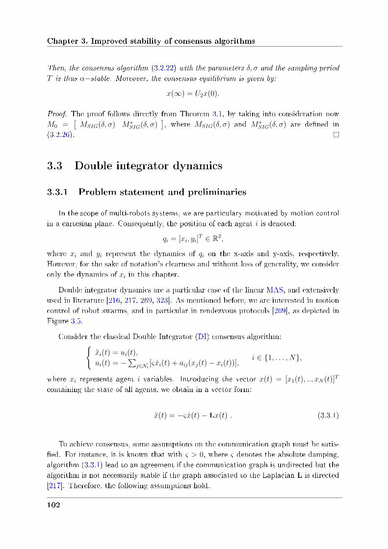
Chapter 3. Improved stability of consensus algorithms
Then, the consensus algorithm (3.2.22) with the parameters 𝛿, 𝜎 and the sampling period
𝑇 is thus 𝛼−stable. Moreover, the consensus equilibrium is given by:
𝑥(∞) = 𝑈2𝑥(0).
Proof. The proof follows directly from Theorem 3.1, by taking into consideration now𝑀0 =
[𝑀𝑆𝐼𝐺(𝛿, 𝜎) 𝑀*
𝑆𝐼𝐺(𝛿, 𝜎)], where 𝑀𝑆𝐼𝐺(𝛿, 𝜎) and 𝑀*
𝑆𝐼𝐺(𝛿, 𝜎) are dened in(3.2.26).
3.3 Double integrator dynamics
3.3.1 Problem statement and preliminaries
In the scope of multi-robots systems, we are particulary motivated by motion controlin a cartesian plane. Consequently, the position of each agent 𝑖 is denoted:
𝑞𝑖 = [𝑥𝑖, 𝑦𝑖]𝑇 ∈ R2,
where 𝑥𝑖 and 𝑦𝑖 represent the dynamics of 𝑞𝑖 on the x-axis and y-axis, respectively.However, for the sake of notation's clearness and without loss of generality, we consideronly the dynamics of 𝑥𝑖 in this chapter.
Double integrator dynamics are a particular case of the linear MAS, and extensivelyused in literature [216, 217, 269, 323]. As mentioned before, we are interested in motioncontrol of robot swarms, and in particular in rendezvous protocols [269], as depicted inFigure 3.5.
Consider the classical Double Integrator (DI) consensus algorithm:𝑖(𝑡) = 𝑢𝑖(𝑡),
𝑢𝑖(𝑡) = −∑𝑗∈𝒩𝑖
[𝜍𝑖(𝑡) + 𝑎𝑖𝑗(𝑥𝑗(𝑡) − 𝑥𝑖(𝑡))],𝑖 ∈ 1, . . . , 𝑁,
where 𝑥𝑖 represents agent 𝑖 variables. Introducing the vector 𝑥(𝑡) = [𝑥1(𝑡), .., 𝑥𝑁(𝑡)]𝑇
containing the state of all agents, we obtain in a vector form:
(𝑡) = −𝜍(𝑡) − L𝑥(𝑡) . (3.3.1)
To achieve consensus, some assumptions on the communication graph must be satis-ed. For instance, it is known that with 𝜍 > 0, where 𝜍 denotes the absolute damping,algorithm (3.3.1) lead to an agreement if the communication graph is undirected but thealgorithm is not necessarily stable if the graph associated to the Laplacian L is directed[217]. Therefore, the following assumptions hold.
102
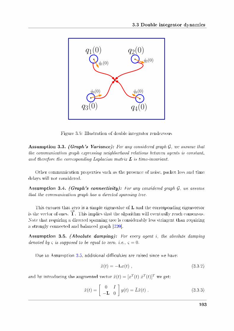
3.3 Double integrator dynamics
q1(0) q2(0)
q3(0) q4(0)
q1(0)q2(0)
q4(0)q3(0)
Figure 3.5: Illustration of double integrator rendezvous
Assumption 3.3. (Graph’s Variance): For any considered graph 𝒢, we assume thatthe communication graph expressing neighborhood relations between agents is constant,
and therefore the corresponding Laplacian matrix L is time-invariant.
Other communication properties such as the presence of noise, packet loss and timedelays will not considered.
Assumption 3.4. (Graph’s connectivity): For any considered graph 𝒢, we assume
that the communication graph has a directed spanning tree.
This ensures that zero is a simple eigenvalue of L and the corresponding eigenvectoris the vector of ones,
−→1 . This implies that the algorithm will eventually reach consensus.
Note that requiring a directed spanning tree is considerably less stringent than requiringa strongly connected and balanced graph [220].
Assumption 3.5. (Absolute damping): For every agent 𝑖, the absolute damping
denoted by 𝜍 is supposed to be equal to zero, i.e., 𝜍 = 0.
Due to Assumption 3.5, additional diculties are raised since we have:
(𝑡) = −L𝑥(𝑡) , (3.3.2)
and by introducing the augmented vector (𝑡) = [𝑥𝑇 (𝑡) 𝑇 (𝑡)]𝑇 we get:
(𝑡) =
[0 𝐼
−L 0
]𝑦(𝑡) = (𝑡) . (3.3.3)
103
Chapter 3. Improved stability of consensus algorithms
It is important to point out that the trace of the matrix is zero whatever the commu-nication graph and that the eigenvalues of L are either on the imaginary axis or thereis at least one eigenvalue on the right side of the imaginary axis. Consequently, thisleads to an oscillatory or unstable behavior of the algorithm. It is precisely this behav-ior that motivates our interest. In fact, since simple integrator consensus algorithm'sperformances can also be improved using an appropriated sampling, as shown in theprevious section, it was our intuition that the benets of such an approach should beeven greater for double integrator dynamics. Indeed, it is important to bring forwardthe technical advantages of Assumption 3.5: by supposing 𝜎 = 0, we reduce drasticallythe information quantity needed for the control laws, and in a technical point of view,no velocity sensors are needed but only sensors to get the agent's position. This meanseconomical, space and calculation savings.
The study of improved stability properties of double integrator consensus algorithmspresented in the sequel will only consider partial memory, using for control agent's owninformation sampled information. However, these results can be easily extended in orderto consider global memory.
3.3.2 Controller design
Using the concept of stabilizing delay, we will consider a sampling delay that was usedin [98, 250] and dened in (3.2.4). It is important to recall that an inherent assumptionis that all agents are synchronized and share the same clock. Using partial memory,algorithm (3.3.2) is modied into a new algorithm dened by:
∀𝑡 ∈ [𝑡𝑘 𝑡𝑘+1[, (𝑡) = −(L + 𝜑2𝐼)𝑥(𝑡) + 𝜑2𝑥(𝑡𝑘) . (3.3.4)
where 𝜑 ∈ R and 𝑇 ≥ 0 are now additional control parameters. Moreover, as for thememory based controller (3.2.5), if 𝜑 and/or 𝑇 are taken as zeros then the respectiveclassical algorithm is retrieved. The structure of controller (3.3.4) is represented inFigure 3.6. It is important at this stage to enhance that (3.3.4) diers from (3.2.5)on the partial information used. More precisely, while in (3.2.5) the information of eachagent's neighbors is incorporated in the controller weighted by the parameter 𝛿, in (3.3.4)each agent 𝑖 uses its own sampled information weighted by the parameter 𝜑. Therefore,the diagonal contribution of the Laplacian is split in two parts: one delayed and theother is kept at the current time.
104
3.3 Double integrator dynamics
-L x(t)
φ2I
+x(t)
tk-+
+1s2
1s2
-L
Figure 3.6: Bloc diagrams of the classical and the improved algorithms with neighboringpartial memory.
3.3.3 Definition of an appropriate model
This section focuses on the denition of a suitable modeling of the consensus algo-rithm for convergence analysis. The next lemma shows an appropriate way to rewrite(3.3.4) based on the properties of L.
Lemma 3.4. (Rodrigues de Campos et al. [231]) The consensus problem (3.3.4) can
be rewritten using 𝑧1 ∈ R𝑁−1, 𝑧2 ∈ R such that:
𝑧1(𝑡) = (Ω − 𝜑2𝐼)𝑧1(𝑡) + 𝜑2𝑧1(𝑡𝑘), (3.3.5a)
𝑧2(𝑡) = −𝜑2𝑧2(𝑡) + 𝜑2𝑧2(𝑡𝑘), (3.3.5b)
where the matrix Ω is given in (3.2.6).
Proof. Consider (3.3.4). It can be rewritten as follows:
∀𝑡 ∈ [𝑡𝑘 𝑡𝑘+1[, (𝑡) = −L𝑥(𝑡) − 𝜑2
∫ 𝑡
𝑡𝑘
(𝑠)𝑑𝑠.
Applying the change of coordinates 𝑧 = 𝑈𝑥 it follows from (3.2.6) that (3.3.4) can berewritten into two equations where 𝑧1 = 𝑈1𝑥 ∈ R(𝑁−1) and 𝑧2 = 𝑈2𝑥 ∈ R𝑁 representrespectively the 𝑁 − 1 rst components and the last component of 𝑧. Noting that𝑈(−𝜑2𝐼)𝑊 = −𝜑2𝐼, (3.3.4) can be rewritten using the Leibnitz formula as:
𝑧1(𝑡) = Ω𝑧1(𝑡) − 𝜑2∫ 𝑡𝑡𝑘1(𝑠)𝑑𝑠,
𝑧2(𝑡) = −𝜑2∫ 𝑡𝑡𝑘2(𝑠)𝑑𝑠.
(3.3.6)
The proof is concluded using∫ 𝑡𝑡𝑘𝑖(𝑠)𝑑𝑠 = 𝑧𝑖(𝑡) − 𝑧𝑖(𝑡𝑘).
Based on change of coordinates presented in (3.2.6), the sampled algorithm (3.3.4) isdecomposed into two components: (i) a vectorial component 𝑧1 associated with non-zero
105
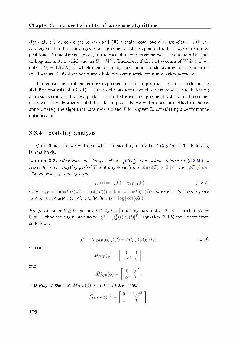
Chapter 3. Improved stability of consensus algorithms
eigenvalues that converges to zero and (ii) a scalar component 𝑧2 associated with thezero eigenvalue that converges to an agreement value dependent ont the system's initialpositions. As mentioned before, in the case of a symmetric network, the matrix 𝑊 is anorthogonal matrix which means 𝑈 = 𝑊 𝑇 . Therefore, if the last column of 𝑊 is 𝛽
−→1 ,we
obtain 𝑈2 = 1/(𝛽𝑁)−→1 , which means that 𝑧2 corresponds to the average of the position
of all agents. This does not always hold for asymmetric communication network.
The consensus problem is now expressed into an appropriate form to perform thestability analysis of (3.3.4). Due to the structure of this new model, the followinganalysis is composed of two parts. The rst studies the agreement value and the seconddeals with the algorithm's stability. More precisely, we will propose a method to chooseappropriately the algorithm parameters 𝜑 and 𝑇 for a given L, considering a performanceoptimisation.
3.3.4 Stability analysis
On a rst step, we will deal with the stability analysis of (3.3.5b). The followinglemma holds.
Lemma 3.5. (Rodrigues de Campos et al. [231]) The system defined in (3.3.5b) is
stable for any sampling period 𝑇 and any 𝜑 such that sin (𝜑𝑇 ) = 0 [𝜋], i.e., 𝜑𝑇 = 𝑘𝜋.
The variable 𝑧2 converges to:
𝑧2(∞) = 𝑧2(0) + 𝛾𝜑𝑇 2(0), (3.3.7)
where 𝛾𝜑𝑇 = sin(𝜑𝑇 )/(𝜑(1− cos(𝜑𝑇 ))) = tan((𝜋−𝜑𝑇 )/2)/𝜑. Moreover, the convergence
rate of the solution to this equilibrium is − log | cos(𝜑𝑇 )|.
Proof. Consider 𝑘 ≥ 0 and any 𝑡 ∈ [𝑡𝑘 𝑡𝑘+1[ and any parameters 𝑇 , 𝜑 such that 𝜑𝑇 =0 [𝜋]. Dene the augmented vector 𝜒* = [𝑧𝑇2 (𝑡) 2(𝑡)]
𝑇 . Equation (3.3.5) can be rewrittenas follows:
𝜒* = 𝐷𝐼𝑃 (𝜑)𝜒*(𝑡) + *𝐷𝐼𝑃 (𝜑)𝜒*(𝑡𝑘), (3.3.8)
where
𝐷𝐼𝑃 (𝜑) =
[0 1
−𝜑2 0
],
and
*𝐷𝐼𝑃 (𝜑) =
[0 0
𝜑2 0
].
It is easy to see that 𝐷𝐼𝑃 (𝜑) is invertible and that:
𝐷𝐼𝑃 (𝜑)−1 =
[0 −1/𝜑2
1 0
].
106
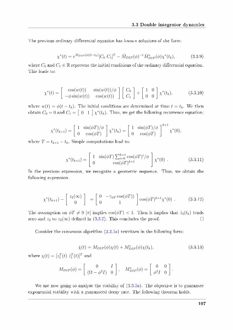
3.3 Double integrator dynamics
The previous ordinary dierential equation has known solutions of the form:
𝜒*(𝑡) = 𝑒𝑀𝐷𝐼𝑃 (𝜑)(𝑡−𝑡𝑘)[𝐶0 𝐶1]𝑇 − 𝐷𝐼𝑃 (𝜑)−1*
𝐷𝐼𝑃 (𝜑)𝜒*(𝑡𝑘), (3.3.9)
where 𝐶0 and 𝐶1 ∈ R represent the initial conditions of the ordinary dierential equation.This leads to:
𝜒*(𝑡) =
[cos(𝑤(𝑡)) sin(𝑤(𝑡))/𝜑
−𝜑 sin(𝑤(𝑡)) cos(𝑤(𝑡))
] [𝐶0
𝐶1
]+
[1 0
0 0
]𝜒*(𝑡𝑘), (3.3.10)
where 𝑤(𝑡) = 𝜑(𝑡 − 𝑡𝑘). The initial conditions are determined at time 𝑡 = 𝑡𝑘. We thenobtain 𝐶0 = 0 and 𝐶1 =
[0 1
]𝜒*(𝑡𝑘). Thus, we get the following recurrence equation:
𝜒*(𝑡𝑘+1) =
[1 sin(𝜑𝑇 )/𝜑
0 cos(𝜑𝑇 )
]𝜒*(𝑡𝑘) =
[1 sin(𝜑𝑇 )/𝜑
0 cos(𝜑𝑇 )
]𝑘+1
𝜒*(0),
where 𝑇 = 𝑡𝑘+1 − 𝑡𝑘. Simple computations lead to:
𝜒*(𝑡𝑘+1) =
[1 sin(𝜑𝑇 )
∑𝑘+1𝑖=0 cos(𝜑𝑇 )𝑖/𝜑
0 cos(𝜑𝑇 )𝑘+1
]𝜒*(0) . (3.3.11)
In the previous expression, we recognize a geometric sequence. Thus, we obtain thefollowing expression:
𝜒*(𝑡𝑘+1) −[𝑧2(∞)
0
]=
[0 −𝛾𝜑𝑇 cos(𝜑𝑇 ))
0 1
]cos(𝜑𝑇 )𝑘+1𝜒*(0) . (3.3.12)
The assumption on 𝜑𝑇 = 0 [𝜋] implies cos(𝜑𝑇 ) < 1. Then it implies that 2(𝑡𝑘) tendszero and 𝑧2 to 𝑧2(∞) dened in (3.3.7). This concludes the proof.
Consider the consensus algorithm (3.3.5a) rewritten in the following form:
(𝑡) = 𝑀𝐷𝐼𝑃 (𝜑)𝜒(𝑡) +𝑀*𝐷𝐼𝑃 (𝜑)𝜒(𝑡𝑘), (3.3.13)
where 𝜒(𝑡) = [𝑧𝑇1 (𝑡) 𝑇1 (𝑡)]𝑇 and
𝑀𝐷𝐼𝑃 (𝜑) =
[0 𝐼
(Ω − 𝜑2𝐼) 0
], 𝑀*
𝐷𝐼𝑃 (𝜑) =
[0 0
𝜑2𝐼 0
].
We are now going to analyse the stability of (3.3.5a). The objective is to guaranteeexponential stability with a guaranteed decay rate. The following theorem holds.
107
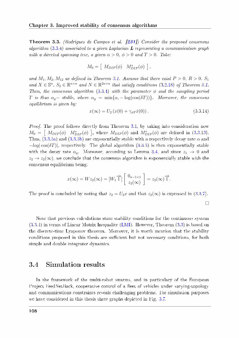
Chapter 3. Improved stability of consensus algorithms
Theorem 3.3. (Rodrigues de Campos et al. [231]) Consider the proposed consensus
algorithm (3.3.4) associated to a given Laplacian L representing a communication graph
with a directed spanning tree, a given 𝛼 > 0, 𝜑 > 0 and 𝑇 > 0. Take:
𝑀0 =[𝑀𝐷𝐼𝑃 (𝜑) 𝑀*
𝐷𝐼𝑃 (𝜑)],
and 𝑀1,𝑀2,𝑀12 as defined in Theorem 3.1. Assume that there exist 𝑃 > 0, 𝑅 > 0, 𝑆1
and 𝑋 ∈ S𝑛, 𝑆2 ∈ R𝑛×𝑛 and 𝑁 ∈ R2𝑛×𝑛 that satisfy conditions (3.2.18) of Theorem 3.1.
Then, the consensus algorithm (3.3.4) with the parameter 𝜑 and the sampling period
𝑇 is thus 𝛼𝑔− stable, where 𝛼𝑔 = min𝛼,− log(cos(𝛿𝑇 )). Moreover, the consensus
equilibrium is given by:
𝑥(∞) = 𝑈2 (𝑥(0) + 𝛾𝜑𝑇 (0)) . (3.3.14)
Proof. The proof follows directly from Theorem 3.1, by taking into consideration now𝑀0 =
[𝑀𝐷𝐼𝑃 (𝜑) 𝑀*
𝐷𝐼𝑃 (𝜑)], where 𝑀𝐷𝐼𝑃 (𝜑) and 𝑀*
𝐷𝐼𝑃 (𝜑) are dened in (3.3.13).Thus, (3.3.5a) and (3.3.5b) are exponentially stable with a respectively decay rate 𝛼 and−𝑙𝑜𝑔| cos(𝛿𝑇 )|, respectively. The global algorithm (3.3.5) is then exponentially stablewith the decay rate 𝛼𝑔. Moreover, according to Lemma 3.4, and since 𝑧1 → 0 and𝑧2 → 𝑧2(∞), we conclude that the consensus algorithm is exponentially stable with theconsensus equilibrium being:
𝑥(∞) = 𝑊𝑧2(∞) = [𝑊1−→1 ]
[0𝑛−1×1
𝑧2(∞)
]= 𝑧2(∞)
−→1 .
The proof is concluded by noting that 𝑧2 = 𝑈2𝑥 and that 𝑧2(∞) is expressed in (3.3.7).
Note that previous calculations state stability conditions for the continuous system(3.3.4) in terms of Linear Matrix Inequality (LMI). However, Theorem (3.3) is based onthe discrete-time Lyaponov theorem. Moreover, it is worth mention that the stabilityconditions proposed in this thesis are sucient but not necessary conditions, for bothsimple and double integrator dynamics.
3.4 Simulation results
In the framework of the multi-robot swarms, and in particulary of the EuropeanProject FeedNetBack, cooperative control of a eet of vehicles under varying-topologyand communications constraints reveals challenging problems. For simulation purposeswe have considered in this thesis three graphs depicted in Fig. 3.7.
108
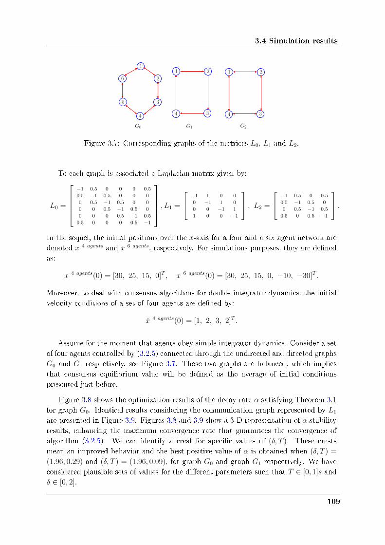
3.4 Simulation results
1
2
3
4
5
6
G0 G1
1 2
34
G2
1 2
34
Figure 3.7: Corresponding graphs of the matrices 𝐿0, 𝐿1 and 𝐿2.
To each graph is associated a Laplacian matrix given by:
𝐿0 =
⎡⎢⎢⎢⎣−1 0.5 0 0 0 0.5
0.5 −1 0.5 0 0 0
0 0.5 −1 0.5 0 0
0 0 0.5 −1 0.5 0
0 0 0 0.5 −1 0.5
0.5 0 0 0 0.5 −1
⎤⎥⎥⎥⎦ , 𝐿1 =
⎡⎣ −1 1 0 0
0 −1 1 0
0 0 −1 1
1 0 0 −1
⎤⎦ , 𝐿2 =
⎡⎣ −1 0.5 0 0.5
0.5 −1 0.5 0
0 0.5 −1 0.5
0.5 0 0.5 −1
⎤⎦ .In the sequel, the initial positions over the 𝑥-axis for a four and a six agent network aredenoted 𝑥 4 𝑎𝑔𝑒𝑛𝑡𝑠 and 𝑥 6 𝑎𝑔𝑒𝑛𝑡𝑠, respectively. For simulations purposes, they are denedas:
𝑥 4 𝑎𝑔𝑒𝑛𝑡𝑠(0) = [30, 25, 15, 0]𝑇 , 𝑥 6 𝑎𝑔𝑒𝑛𝑡𝑠(0) = [30, 25, 15, 0, −10, −30]𝑇 .
Moreover, to deal with consensus algorithms for double integrator dynamics, the initialvelocity conditions of a set of four agents are dened by:
4 𝑎𝑔𝑒𝑛𝑡𝑠(0) = [1, 2, 3, 2]𝑇 .
Assume for the moment that agents obey simple integrator dynamics. Consider a setof four agents controlled by (3.2.5) connected through the undirected and directed graphs𝐺0 and 𝐺1 respectively, see Figure 3.7. Those two graphs are balanced, which impliesthat consensus equilibrium value will be dened as the average of initial conditionspresented just before.
Figure 3.8 shows the optimization results of the decay rate 𝛼 satisfying Theorem 3.1for graph 𝐺0. Identical results considering the communication graph represented by 𝐿1
are presented in Figure 3.9. Figures 3.8 and 3.9 show a 3-D representation of 𝛼 stabilityresults, enhancing the maximum convergence rate that guarantees the convergence ofalgorithm (3.2.5). We can identify a crest for specic values of (𝛿, 𝑇 ). These crestsmean an improved behavior and the best positive value of 𝛼 is obtained when (𝛿, 𝑇 ) =
(1.96, 0.29) and (𝛿, 𝑇 ) = (1.96, 0.09), for graph 𝐺0 and graph 𝐺1 respectively. We haveconsidered plausible sets of values for the dierent parameters such that 𝑇 ∈ [0, 1]𝑠 and𝛿 ∈ [0, 2].
109
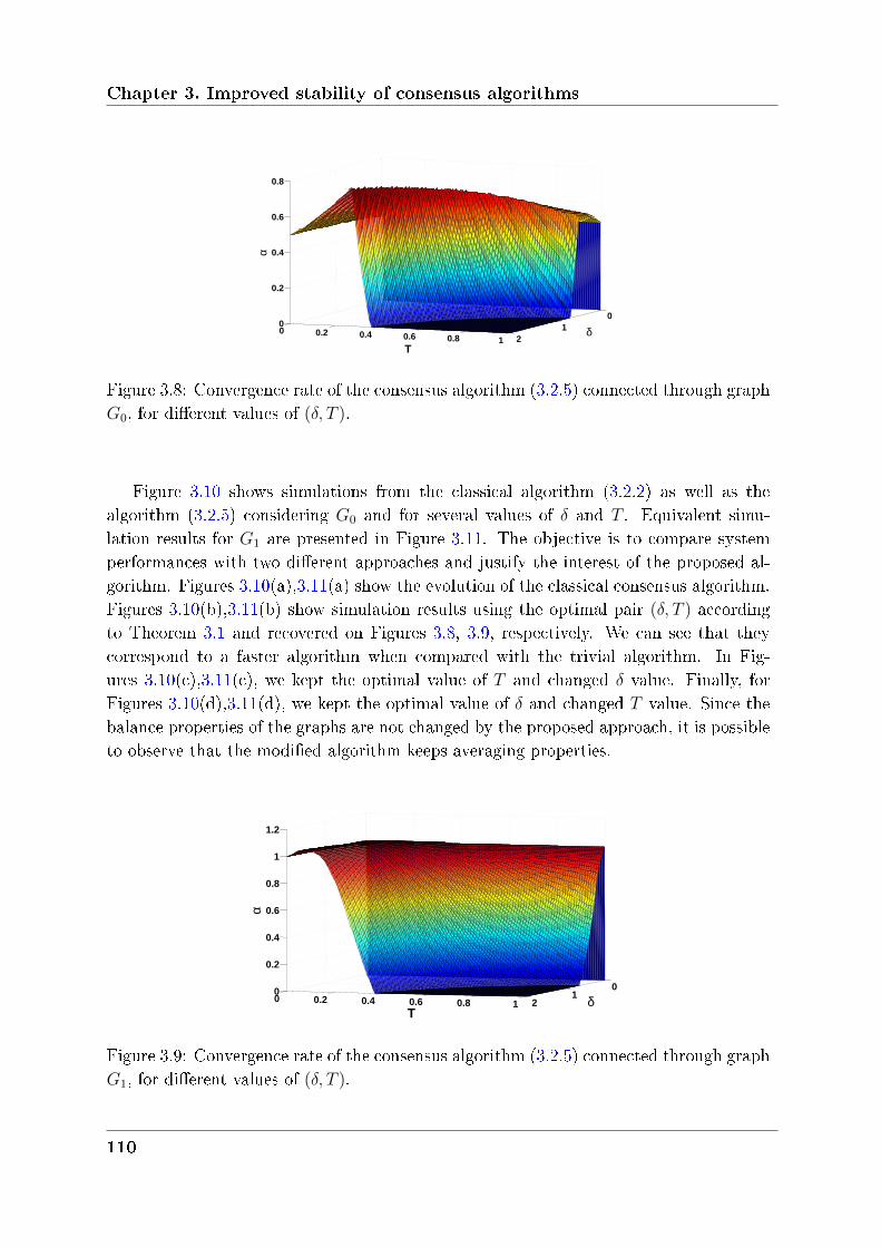
Chapter 3. Improved stability of consensus algorithms
01
20 0.2 0.4 0.6 0.8 1
0
0.2
0.4
0.6
0.8
α
δT
Figure 3.8: Convergence rate of the consensus algorithm (3.2.5) connected through graph𝐺0, for dierent values of (𝛿, 𝑇 ).
Figure 3.10 shows simulations from the classical algorithm (3.2.2) as well as thealgorithm (3.2.5) considering 𝐺0 and for several values of 𝛿 and 𝑇 . Equivalent simu-lation results for 𝐺1 are presented in Figure 3.11. The objective is to compare systemperformances with two dierent approaches and justify the interest of the proposed al-gorithm. Figures 3.10(a),3.11(a) show the evolution of the classical consensus algorithm.Figures 3.10(b),3.11(b) show simulation results using the optimal pair (𝛿, 𝑇 ) accordingto Theorem 3.1 and recovered on Figures 3.8, 3.9, respectively. We can see that theycorrespond to a faster algorithm when compared with the trivial algorithm. In Fig-ures 3.10(c),3.11(c), we kept the optimal value of 𝑇 and changed 𝛿 value. Finally, forFigures 3.10(d),3.11(d), we kept the optimal value of 𝛿 and changed 𝑇 value. Since thebalance properties of the graphs are not changed by the proposed approach, it is possibleto observe that the modied algorithm keeps averaging properties.
01
20 0.2 0.4 0.6 0.8 10
0.2
0.4
0.6
0.8
1
1.2
T
α
Tδ
Figure 3.9: Convergence rate of the consensus algorithm (3.2.5) connected through graph𝐺1, for dierent values of (𝛿, 𝑇 ).
110
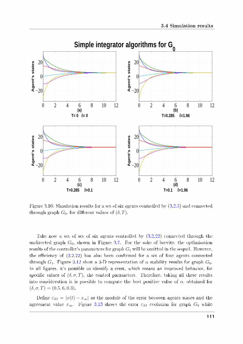
3.4 Simulation results
0 2 4 6 8 10 12
−20
0
20
Ag
en
t‘s s
tate
s
(a)T= 0 δ= 0
0 2 4 6 8 10 12
−20
0
20
Ag
en
t‘s s
tate
s
(b)T=0.285 δ=1.96
0 2 4 6 8 10 12
−20
0
20
Ag
en
t‘s s
tate
s
(c)T=0.285 δ=0.1
0 2 4 6 8 10 12
−20
0
20
Ag
en
t‘s s
tate
s
(d)T=0.1 δ=1.96
Simple integrator algorithms for G0
Figure 3.10: Simulation results for a set of six agents controlled by (3.2.5) and connectedthrough graph 𝐺0, for dierent values of (𝛿, 𝑇 ).
Take now a set of set of six agents controlled by (3.2.22) connected through theundirected graph 𝐺0, shown in Figure 3.7. For the sake of brevity, the optimisationresults of the controller's parameters for graph 𝐺1 will be omitted in the sequel. However,the eciency of (3.2.22) has also been conrmed for a set of four agents connectedthrough 𝐺1. Figure 3.12 show a 3-D representation of 𝛼 stability results for graph 𝐺0.In all gures, it's possible to identify a crest, which means an improved behavior, forspecic values of (𝛿, 𝜎, 𝑇 ), the control parameters. Therefore, taking all these resultsinto consideration it is possible to compute the best positive value of 𝛼, obtained for(𝛿, 𝜎, 𝑇 ) = (0.5, 6, 0.3).
Dene 𝜀𝑆𝐼 = |𝑥(𝑡) − 𝑥∞| as the module of the error between agents states and theagreement value 𝑥∞. Figure 3.13 shows the error 𝜀𝑆𝐼 evolution for graph 𝐺0 while
111
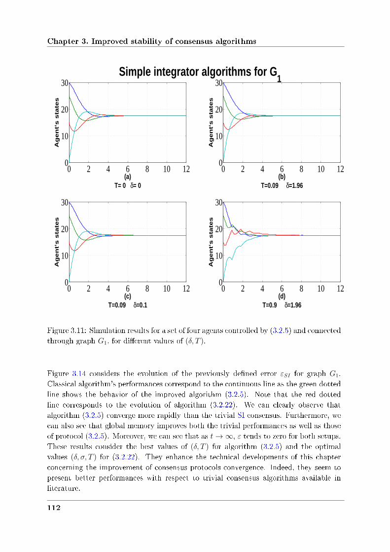
Chapter 3. Improved stability of consensus algorithms
0 2 4 6 8 10 120
10
20
30
Ag
en
t‘s s
tate
s
(a)T= 0 δ= 0
0 2 4 6 8 10 120
10
20
30
Ag
en
t‘s s
tate
s
(b)T=0.09 δ=1.96
0 2 4 6 8 10 120
10
20
30
Ag
en
t‘s s
tate
s
(c)T=0.09 δ=0.1
0 2 4 6 8 10 120
10
20
30A
gen
t‘s s
tate
s
(d)T=0.9 δ=1.96
Simple integrator algorithms for G1
Figure 3.11: Simulation results for a set of four agents controlled by (3.2.5) and connectedthrough graph 𝐺1, for dierent values of (𝛿, 𝑇 ).
Figure 3.14 considers the evolution of the previously dened error 𝜀𝑆𝐼 for graph 𝐺1.Classical algorithm's performances correspond to the continuous line as the green dottedline shows the behavior of the improved algorithm (3.2.5). Note that the red dottedline corresponds to the evolution of algorithm (3.2.22). We can clearly observe thatalgorithm (3.2.5) converge more rapidly than the trivial SI consensus. Furthermore, wecan also see that global memory improves both the trivial performances as well as thoseof protocol (3.2.5). Moreover, we can see that as 𝑡→ ∞, 𝜀 tends to zero for both setups.These results consider the best values of (𝛿, 𝑇 ) for algorithm (3.2.5) and the optimalvalues (𝛿, 𝜎, 𝑇 ) for (3.2.22). They enhance the technical developments of this chapterconcerning the improvement of consensus protocols convergence. Indeed, they seem topresent better performances with respect to trivial consensus algorithms available inliterature.
112
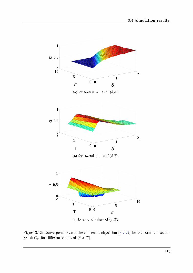
3.4 Simulation results
01
2
05
100
0.5
1
δσ
α
(a) for several values of (𝛿, 𝜎)
01
2
01
20
0.5
1
δT
α
(b) for several values of (𝛿, 𝑇 )
05
10
01
20
0.5
1
σT
α
(c) for several values of (𝜎, 𝑇 )
Figure 3.12: Convergence rate of the consensus algorithm (3.2.22) for the communicationgraph 𝐺0, for dierent values of (𝛿, 𝜎, 𝑇 ).
113
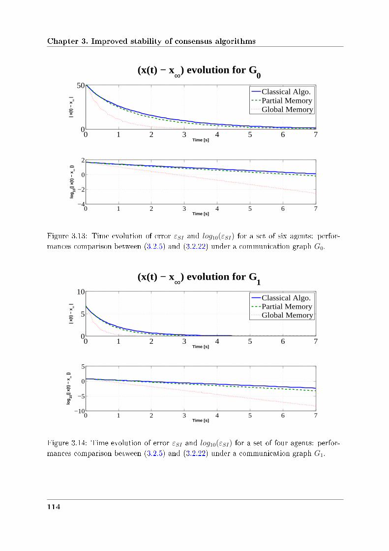
Chapter 3. Improved stability of consensus algorithms
0 1 2 3 4 5 6 70
50
Time [s]
| x(t)
− x
∞ |
(x(t) − x∞) evolution for G0
Classical Algo.Partial MemoryGlobal Memory
0 1 2 3 4 5 6 7−4
−2
0
2
log
10(|
x(t)
− x
∞ |)
Time [s]
Figure 3.13: Time evolution of error 𝜀𝑆𝐼 and 𝑙𝑜𝑔10(𝜀𝑆𝐼) for a set of six agents: perfor-mances comparison between (3.2.5) and (3.2.22) under a communication graph 𝐺0.
0 1 2 3 4 5 6 70
5
10
Time [s]
| x(t)
− x
∞ |
(x(t) − x∞) evolution for G1
Classical Algo.Partial MemoryGlobal Memory
0 1 2 3 4 5 6 7−10
−5
0
5
log
10(|
x(t)
− x
∞ |)
Time [s]
Figure 3.14: Time evolution of error 𝜀𝑆𝐼 and 𝑙𝑜𝑔10(𝜀𝑆𝐼) for a set of four agents: perfor-mances comparison between (3.2.5) and (3.2.22) under a communication graph 𝐺1.
114
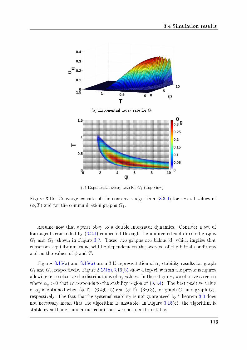
3.4 Simulation results
05
10
00.511.50
0.1
0.2
0.3
0.4
φT
α g
(a) Exponential decay rate for 𝐺1
0 2 4 6 8 100
0.5
1
1.5 αg
φ
T
0
0.05
0.1
0.15
0.2
0.25
0.3
(b) Exponential decay rate for 𝐺1 (Top view)
Figure 3.15: Convergence rate of the consensus algorithm (3.3.4) for several values of(𝜑, 𝑇 ) and for the communication graphs 𝐺1.
Assume now that agents obey to a double integrator dynamics. Consider a set offour agents controlled by (3.3.4) connected through the undirected and directed graphs𝐺1 and 𝐺2, shown in Figure 3.7. These two graphs are balanced, which implies thatconsensus equilibrium value will be dependent on the average of the initial conditionsand on the values of 𝜑 and 𝑇 .
Figures 3.15(a) and 3.16(a) are a 3-D representation of 𝛼𝑔 stability results for graph𝐺1 and 𝐺2, respectively. Figure 3.15(b),3.16(b) show a top-view from the previous guresallowing us to observe the distributions of 𝛼𝑔 values. In these gures, we observe a regionwhere 𝛼𝑔 > 0 that corresponds to the stability region of (3.3.4). The best positive valueof 𝛼𝑔 is obtained when (𝜑,T)=(6.4;0.15) and (𝜑,T)=(3;0.3), for graph 𝐺1 and graph 𝐺2,respectively. The fact thatthe systems' stability is not guaranteed by Theorem 3.3 doesnot necessary mean that the algorithm is unstable: in Figure 3.18(c), the algorithm isstable even though under our conditions we consider it unstable.
115
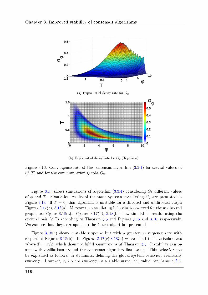
Chapter 3. Improved stability of consensus algorithms
05
10
00.511.50
0.2
0.4
0.6
φT
α g
(a) Exponential decay rate for 𝐺2
0 2 4 6 8 100
0.5
1
1.5 αg
φ
T
0
0.1
0.2
0.3
0.4
0.5
(b) Exponential decay rate for 𝐺2 (Top view)
Figure 3.16: Convergence rate of the consensus algorithm (3.3.4) for several values of(𝜑, 𝑇 ) and for the communication graphs 𝐺2.
Figure 3.17 shows simulations of algorithm (3.3.4) considering 𝐺1 dierent valuesof 𝜑 and 𝑇 . Simulation results of the same systems considering 𝐺2 are presented inFigure 3.18. If 𝑇 = 0, this algorithm is unstable for a directed and undirected graphFigures 3.17(a), 3.18(a). Moreover, an oscillating behavior is observed for the undirectedgraph, see Figure 3.18(a). Figures 3.17(b), 3.18(b) show simulation results using theoptimal pair (𝜑,T) according to Theorem 3.3 and Figures 3.15 and 3.16, respectively.We can see that they correspond to the fastest algorithm presented.
Figure 3.18(c) shows a stable response but with a greater convergence rate withrespect to Figures 3.18(b). In Figures 3.17(c),3.18(d) we can nd the particular casewhere 𝑇 = 𝜋/𝜑, which does not fulll assumptions of Theorem 3.3. Instability can beseen with oscillations around the consensus algorithm nal value. This behavior canbe explained as follows: 𝑧1 dynamics, dening the global system behavior, eventuallyconverge. However, 𝑧2 do not converge to a stable agreement value, see Lemma 3.5.
116
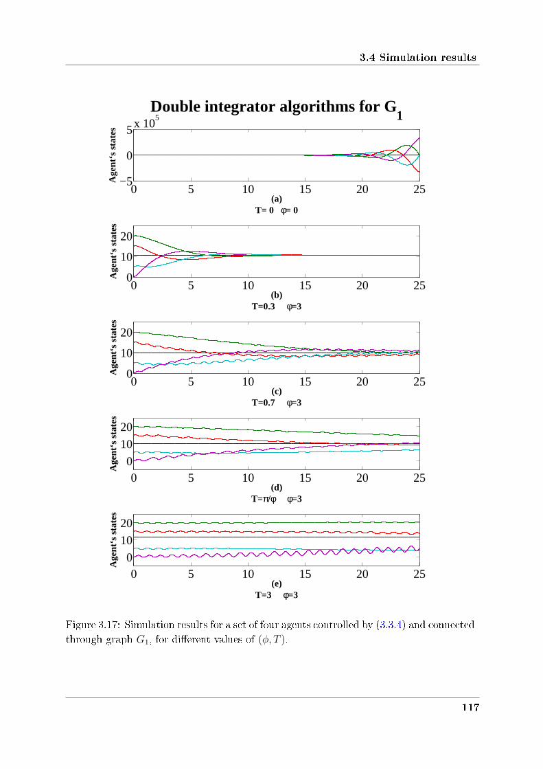
3.4 Simulation results
0 5 10 15 20 25−5
0
5x 10⁵
Double integrator algorithms for G1
(a)T= 0 φ= 0
Age
nt‘s
sta
tes
0 5 10 15 20 250
10
20
Age
nt‘s
sta
tes
(b)T=0.3 φ=3
0 5 10 15 20 250
10
20
Age
nt‘s
sta
tes
(c)T=0.7 φ=3
0 5 10 15 20 250
10
20
Age
nt‘s
sta
tes
(d)T=π/φ φ=3
0 5 10 15 20 250
10
20
Age
nt‘s
sta
tes
(e)T=3 φ=3
Figure 3.17: Simulation results for a set of four agents controlled by (3.3.4) and connectedthrough graph 𝐺1, for dierent values of (𝜑, 𝑇 ).
117
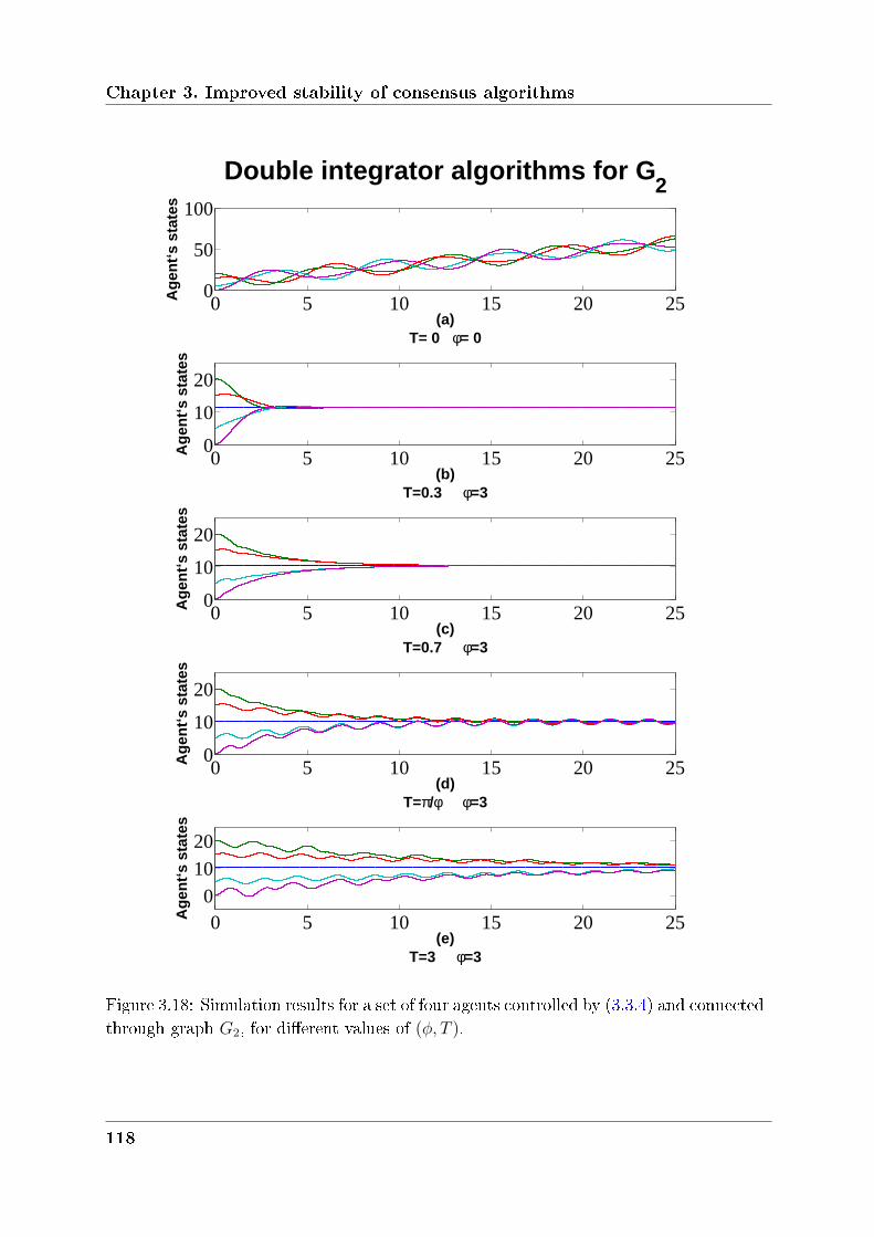
Chapter 3. Improved stability of consensus algorithms
0 5 10 15 20 250
50
100
Double integrator algorithms for G2
(a)T= 0 φ= 0
Ag
ent‘
s st
ates
0 5 10 15 20 250
10
20
Ag
ent‘
s st
ates
(b)T=0.3 φ=3
0 5 10 15 20 250
10
20
Ag
ent‘
s st
ates
(c)T=0.7 φ=3
0 5 10 15 20 250
10
20
Ag
ent‘
s st
ates
(d)T=π/φ φ=3
0 5 10 15 20 250
10
20
Ag
ent‘
s st
ates
(e)T=3 φ=3
Figure 3.18: Simulation results for a set of four agents controlled by (3.3.4) and connectedthrough graph 𝐺2, for dierent values of (𝜑, 𝑇 ).
118
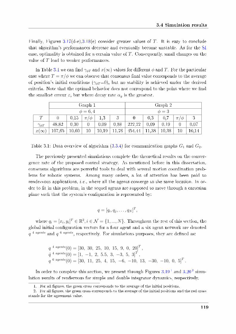
3.4 Simulation results
Finally, Figures 3.17(d-e),3.18(e) consider greater values of 𝑇 . It is easy to concludethat algorithm's performances decrease and eventually become unstable. As for the SIcase, optimality is obtained for a certain value of 𝑇 . Consequently, small changes on thevalue of 𝑇 lead to weaker performances.
In Table 3.1 we can nd 𝛾𝜑𝑇 and 𝑥(∞) values for dierent 𝜑 and 𝑇 . For the particularcase where 𝑇 = 𝜋/𝜑 we can observe that consensus nal value corresponds to the averageof position's initial conditions (𝛾𝜑𝑇=0), but no stability is achieved under the derivedcriteria. Note that the optimal behavior does not correspond to the point where we ndthe smallest erreur 𝜀, but where decay rate 𝛼𝑔 is the greatest.
Graph 1 Graph 2𝜑 = 6, 4 𝜑 = 3
𝑇 0 0,15 𝜋/𝜑 1,3 3 0 0,3 0,7 𝜋/𝜑 3𝛾𝜑𝑇 48,82 0,30 0 0,09 0,88 222,22 0,69 0,19 0 0,07𝑥(∞) 107,65 10,60 10 10,19 11,76 454,44 11,38 10,38 10 10,14
Table 3.1: Data overview of algorithm (3.3.4) for communication graphs 𝐺1 and 𝐺2.
The previously presented simulations complete the theoretical results on the conver-gence rate of the proposed control strategy. As mentioned before in this dissertation,consensus algorithms are powerful tools to deal with several motion coordination prob-lems for robotic systems. Among many orders, a lot of attention has been paid torendezvous applications, i.e., where all the agents converge to the same location. In or-der to t in this problem, in the sequel agents are supposed to move through a cartesianplane such that the system's conguration is represented by:
𝑞 = [𝑞𝑖, 𝑞𝑗, . . . , 𝑞𝑁 ]𝑇 ,
where 𝑞𝑖 = [𝑥𝑖, 𝑦𝑖]𝑇 ∈ R2, 𝑖 ∈ 𝒩 = 1, ..., 𝑁. Throughout the rest of this section, the
global initial conguration vectors for a four agent and a six agent network are denoted𝑞 4 𝑎𝑔𝑒𝑛𝑡𝑠 and 𝑞 6 𝑎𝑔𝑒𝑛𝑡𝑠, respectively. For simulations purposes, they are dened as:
𝑞 4 𝑎𝑔𝑒𝑛𝑡𝑠(0) = [30, 30, 25, 10, 15, 9, 0, 20]𝑇 ,
𝑞 4 𝑎𝑔𝑒𝑛𝑡𝑠(0) = [1, −1, 2, 5.5, 3, −3, 5, 3]𝑇 ,
𝑞 6 𝑎𝑔𝑒𝑛𝑡𝑠(0) = [30, 11, 25, 4, 15, −6, −10, 13, −30, −10, 0, 5]𝑇 .
In order to complete this section, we present through Figures 3.19 1 and 3.20 2 simu-lation results of rendezvous for simple and double integrator dynamics, respectively.
1. For all figures, the green cross corresponds to the average of the initial positions.2. For all figures, the green cross corresponds to the average of the initial positions and the red cross
stands for the agreement value.
119
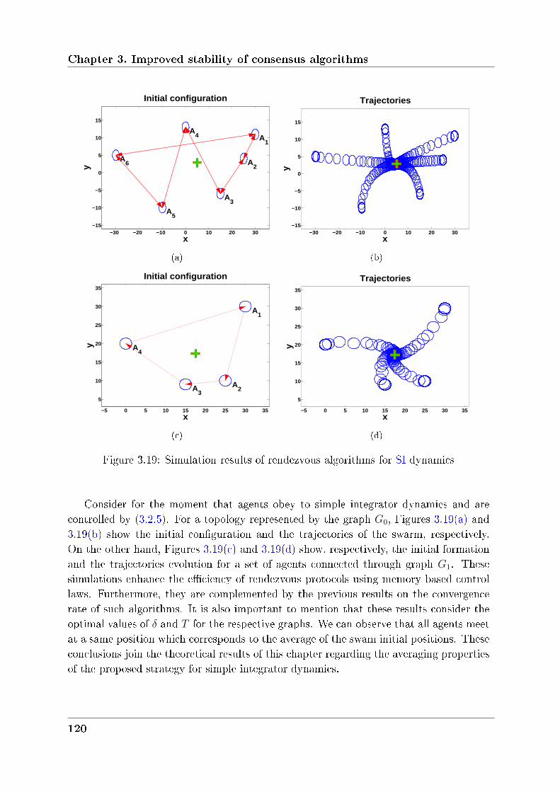
Chapter 3. Improved stability of consensus algorithms
−30 −20 −10 0 10 20 30−15
−10
−5
0
5
10
15
A1
A2
A3
A4
A5
A6
x
yInitial configuration
(a)
−30 −20 −10 0 10 20 30−15
−10
−5
0
5
10
15
x
y
Trajectories
(b)
−5 0 5 10 15 20 25 30 35
5
10
15
20
25
30
35
A1
A2A
3
A4
x
y
Initial configuration
(c)
−5 0 5 10 15 20 25 30 35
5
10
15
20
25
30
35
x
yTrajectories
(d)
Figure 3.19: Simulation results of rendezvous algorithms for SI dynamics
Consider for the moment that agents obey to simple integrator dynamics and arecontrolled by (3.2.5). For a topology represented by the graph 𝐺0, Figures 3.19(a) and3.19(b) show the initial conguration and the trajectories of the swarm, respectively.On the other hand, Figures 3.19(c) and 3.19(d) show, respectively, the initial formationand the trajectories evolution for a set of agents connected through graph 𝐺1. Thesesimulations enhance the eciency of rendezvous protocols using memory based controllaws. Furthermore, they are complemented by the previous results on the convergencerate of such algorithms. It is also important to mention that these results consider theoptimal values of 𝛿 and 𝑇 for the respective graphs. We can observe that all agents meetat a same position which corresponds to the average of the swam initial positions. Theseconclusions join the theoretical results of this chapter regarding the averaging propertiesof the proposed strategy for simple integrator dynamics.
120
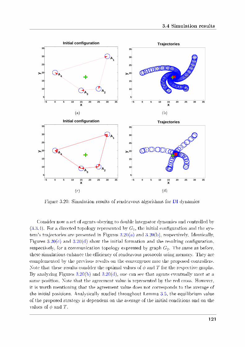
3.4 Simulation results
−5 0 5 10 15 20 25 30 35
5
10
15
20
25
30
35
A1
A2A
3
A4
x
yInitial configuration
(a)
−5 0 5 10 15 20 25 30 35
5
10
15
20
25
30
35
x
y
Trajectories
(b)
−5 0 5 10 15 20 25 30 35
5
10
15
20
25
30
35
A1
A2A
3
A4
x
y
Initial configuration
(c)
−5 0 5 10 15 20 25 30 35
5
10
15
20
25
30
35
x
yTrajectories
(d)
Figure 3.20: Simulation results of rendezvous algorithms for DI dynamics
Consider now a set of agents obeying to double integrator dynamics and controlled by(3.3.4). For a directed topology represented by 𝐺1, the initial conguration and the sys-tem's trajectories are presented in Figures 3.20(a) and 3.20(b), respectively. Identically,Figures 3.20(c) and 3.20(d) show the initial formation and the resulting conguration,respectively, for a communication topology expressed by graph 𝐺2. The same as before,these simulations enhance the eciency of rendezvous protocols using memory. They arecomplemented by the previous results on the convergence rate the proposed controllers.Note that these results consider the optimal values of 𝜑 and 𝑇 for the respective graphs.By analyzing Figures 3.20(b) and 3.20(d), one can see that agents eventually meet at asame position. Note that the agreement value is represented by the red cross. However,it is worth mentioning that the agreement value does not corresponds to the average ofthe initial positions. Analytically studied throughout Lemma 3.5, the equilibrium valueof the proposed strategy is dependent on the average of the initial conditions and on thevalues of 𝜑 and 𝑇 .
121
Chapter 3. Improved stability of consensus algorithms
3.5 Conclusions
In this chapter, the incorporation of memory in consensus controllers for both sim-ple and double integrator consensus dynamics has been studied. The objective was topropose and analyse an eective approach to accelerate the convergence of synchronousdistributed averaging algorithms. In a rst part, the inuence of both local memoryand global memory in consensus algorithms for simple integrator agents have been stud-ied. We could conclude that using global memory drastically improves performanceswhen compared to both trivial and partial memory based algorithms. An optimizationmethod of controller parameters is proposed so that exponential stability of the solutionsis achieved based on the discrete-time Lyaponov theorem and expressed in terms of LMI.Also, analytical conditions for improved performances based on Laplacian's eigenvalueshave been provided. Simulation results show the eciency of the proposed algorithm,as well as the conservation of averaging properties. In a second step, a new consensusalgorithm (3.3.4) for double integrator agents was proposed. This chapter puts forwardthe technical advantages of such a protocol since it reduces information quantity neededfor control: because there is no need for velocity sensors, there are economical, space andcalculation savings. An optimisation of controller parameters is proposed so that expo-nential stability of the solutions is achieved. An expression of the consensus equilibriumis derived with respect to the initial position and velocity of the swarm.
The Laplacian and its spectral properties play a crucial role in convergence analysisof consensus and alignment algorithms. In order to answer the question if it is possibleto increase the convergence speed of a consensus algorithms, this chapter presents ourcontribution to this topic by showing how memory can be incorporated in the controllers.
122
Chapter 4
Control strategies for multi-agent
systems compact formations
Contents
4.1 Context . . . . . . . . . . . . . . . . . . . . . . . . . . . . . . . 124
4.2 Problem statement and preliminaries . . . . . . . . . . . . . 130
4.2.1 System description . . . . . . . . . . . . . . . . . . . . . . . . . 130
4.2.2 Definition of the potential functions . . . . . . . . . . . . . . . 133
4.3 Dispersion algorithm . . . . . . . . . . . . . . . . . . . . . . . 135
4.3.1 Controller design . . . . . . . . . . . . . . . . . . . . . . . . . . 135
4.3.2 Stability analysis . . . . . . . . . . . . . . . . . . . . . . . . . . 137
4.4 Compactness controller . . . . . . . . . . . . . . . . . . . . . . 139
4.4.1 Controller design . . . . . . . . . . . . . . . . . . . . . . . . . . 139
4.4.2 Stability analysis . . . . . . . . . . . . . . . . . . . . . . . . . . 141
4.4.3 Improved controller with variable gain . . . . . . . . . . . . . . 146
4.5 Sequential controller . . . . . . . . . . . . . . . . . . . . . . . . 149
4.5.1 Controller design . . . . . . . . . . . . . . . . . . . . . . . . . . 150
4.5.2 Stability analysis . . . . . . . . . . . . . . . . . . . . . . . . . . 151
4.6 Simulation results . . . . . . . . . . . . . . . . . . . . . . . . . 152
4.7 Conclusions . . . . . . . . . . . . . . . . . . . . . . . . . . . . . 155
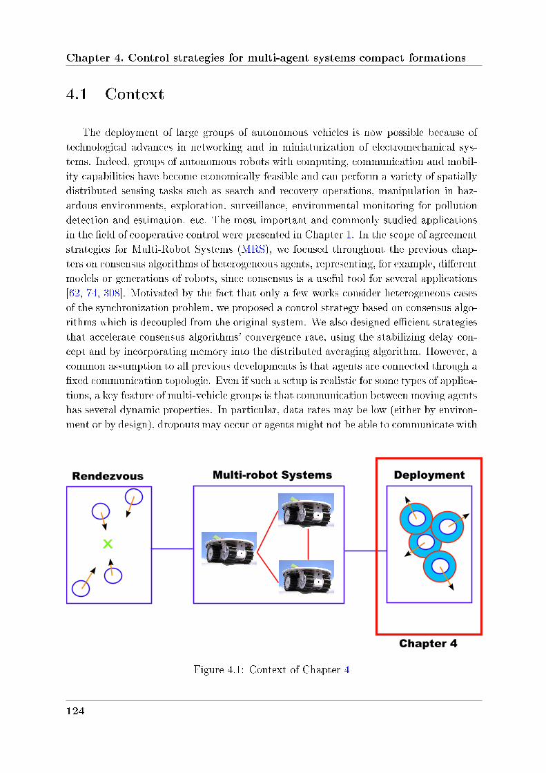
Chapter 4. Control strategies for multi-agent systems compact formations
4.1 Context
The deployment of large groups of autonomous vehicles is now possible because oftechnological advances in networking and in miniaturization of electromechanical sys-tems. Indeed, groups of autonomous robots with computing, communication and mobil-ity capabilities have become economically feasible and can perform a variety of spatiallydistributed sensing tasks such as search and recovery operations, manipulation in haz-ardous environments, exploration, surveillance, environmental monitoring for pollutiondetection and estimation. etc. The most important and commonly studied applicationsin the eld of cooperative control were presented in Chapter 1. In the scope of agreementstrategies for Multi-Robot Systems (MRS), we focused throughout the previous chap-ters on consensus algorithms of heterogeneous agents, representing, for example, dierentmodels or generations of robots, since consensus is a useful tool for several applications[62, 74, 308]. Motivated by the fact that only a few works consider heterogeneous casesof the synchronization problem, we proposed a control strategy based on consensus algo-rithms which is decoupled from the original system. We also designed ecient strategiesthat accelerate consensus algorithms' convergence rate, using the stabilizing delay con-cept and by incorporating memory into the distributed averaging algorithm. However, acommon assumption to all previous developments is that agents are connected through axed communication topologie. Even if such a setup is realistic for some types of applica-tions, a key feature of multi-vehicle groups is that communication between moving agentshas several dynamic properties. In particular, data rates may be low (either by environ-ment or by design), dropouts may occur or agents might not be able to communicate with
Multi-robot Systems
x
Rendezvous Deployment
Chapter 4
Figure 4.1: Context of Chapter 4
124
4.1 Context
all nodes. In the sequel we consider this last setup. More precisely, we consider that dur-ing a coordinated motion or a collaborative task, the interconnections between the agentscan evolve such that new communication links are created and others are broken. Thissetup has important repercussions from both a theoretical and practical point of view.In order to deal with such challenging cases, agents might be coupled by simple rules in-cluding nearest-neighbor or range-based neighborhoods [31, 66, 71, 79, 78, 194, 206, 240].Flocking motions based on nearest-neighbor interaction rules have been developed fordouble-integrator dynamics of the agents [191, 279, 280] and rendezvous algorithms forMulti-Agent Systems (MAS) with limited sensing ranges studied in [87, 148, 150, 151].Furthermore, and extending the results of [163], multi-agent ocking with random com-munication radius was recently studied in [162]. Considering that the communicationnetwork is determined by a metric rule based on a random interaction range, authorsdetermine practical conditions (on the initial positions and velocities of agents) ensur-ing that the agents eventually agree with some probability on a common velocity, i.e.,ocking.
Recently achievements have shown that teams of mobile autonomous agents need notonly agree on some quantity of interest, but also to have the ability to deploy over aregion, assuming a specied pattern, or move in a synchronized manner. While previouschapters considered the rst challenge, oering alternative and innovative agreementstrategies to deal with commonly used MAS applications such as rendezvous, in thischapter we are mainly interested in motion and formation control, since to accomplishexploration, surveillance or rescue tasks, a recurrent choice is to coordinate the agentsto form a particular conguration that satisfy certain local (e.g. node degree) and/orglobal (e.g. network connectivity) constraints, see Figure 4.1.
Widely spread in Nature, motion coordination is a useful tool for groups of vehicles,mobile sensors, and embedded robotic systems. Achieving a coordination task corre-sponds to moving the agents and changing their state to maximize or minimize a specicobjective function. For instance, algorithms for placing individual network nodes withlimited communication range into the environment, while guaranteeing certain commu-nication properties of the resulting node ensemble have been proposed in [62, 63]. Undera bounded tracking error assumption, in [48, 85] the authors show that the formationerror is stabilized when applied to rigid body constrained motions. In [208] controllaws are based on probabilistic node degree constraints, whereas in [24, 25], the authorsconsidered direction-based algorithms. There is a huge number of contributions to thistopic. Even though several other approaches exist in literature, they are not going to bedetailed in this dissertation. However, we present in the sequel some pertinent problemsand related references. Illustrations of these behaviors are presented in Figure 4.2.
125
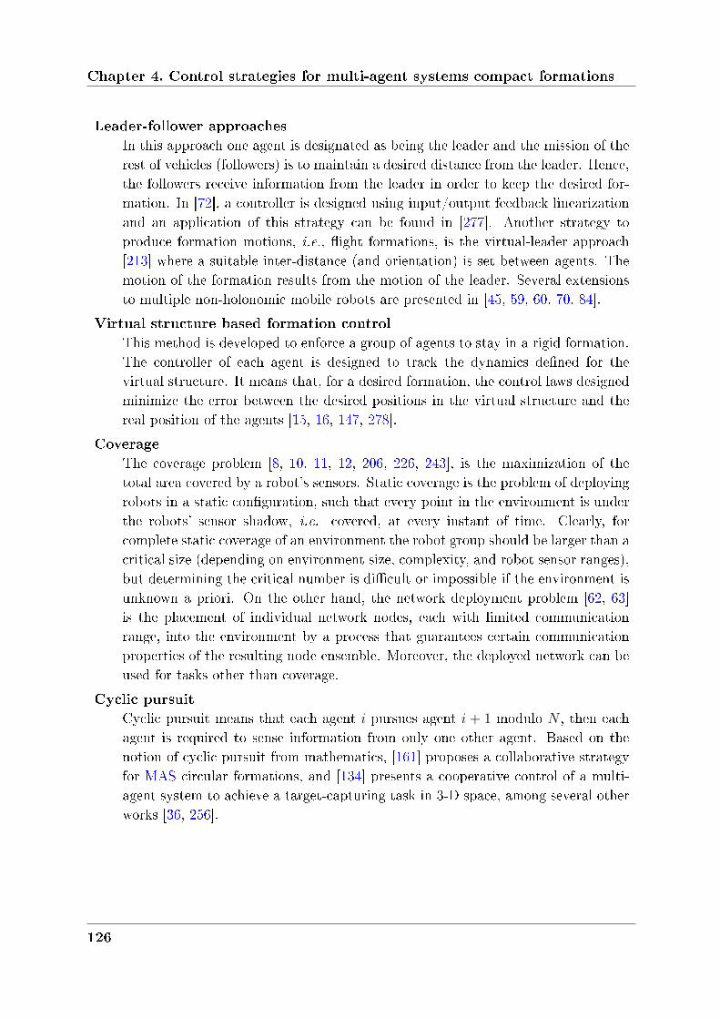
Chapter 4. Control strategies for multi-agent systems compact formations
Leader-follower approaches
In this approach one agent is designated as being the leader and the mission of therest of vehicles (followers) is to maintain a desired distance from the leader. Hence,the followers receive information from the leader in order to keep the desired for-mation. In [72], a controller is designed using input/output feedback linearizationand an application of this strategy can be found in [277]. Another strategy toproduce formation motions, i.e., ight formations, is the virtual-leader approach[213] where a suitable inter-distance (and orientation) is set between agents. Themotion of the formation results from the motion of the leader. Several extensionsto multiple non-holonomic mobile robots are presented in [45, 59, 60, 70, 84].
Virtual structure based formation control
This method is developed to enforce a group of agents to stay in a rigid formation.The controller of each agent is designed to track the dynamics dened for thevirtual structure. It means that, for a desired formation, the control laws designedminimize the error between the desired positions in the virtual structure and thereal position of the agents [15, 16, 147, 278].
Coverage
The coverage problem [8, 10, 11, 12, 206, 226, 243], is the maximization of thetotal area covered by a robot's sensors. Static coverage is the problem of deployingrobots in a static conguration, such that every point in the environment is underthe robots' sensor shadow, i.e. covered, at every instant of time. Clearly, forcomplete static coverage of an environment the robot group should be larger than acritical size (depending on environment size, complexity, and robot sensor ranges),but determining the critical number is dicult or impossible if the environment isunknown a priori. On the other hand, the network deployment problem [62, 63]is the placement of individual network nodes, each with limited communicationrange, into the environment by a process that guarantees certain communicationproperties of the resulting node ensemble. Moreover, the deployed network can beused for tasks other than coverage.
Cyclic pursuit
Cyclic pursuit means that each agent 𝑖 pursues agent 𝑖 + 1 modulo 𝑁 , then eachagent is required to sense information from only one other agent. Based on thenotion of cyclic pursuit from mathematics, [161] proposes a collaborative strategyfor MAS circular formations, and [134] presents a cooperative control of a multi-agent system to achieve a target-capturing task in 3-D space, among several otherworks [36, 256].
126
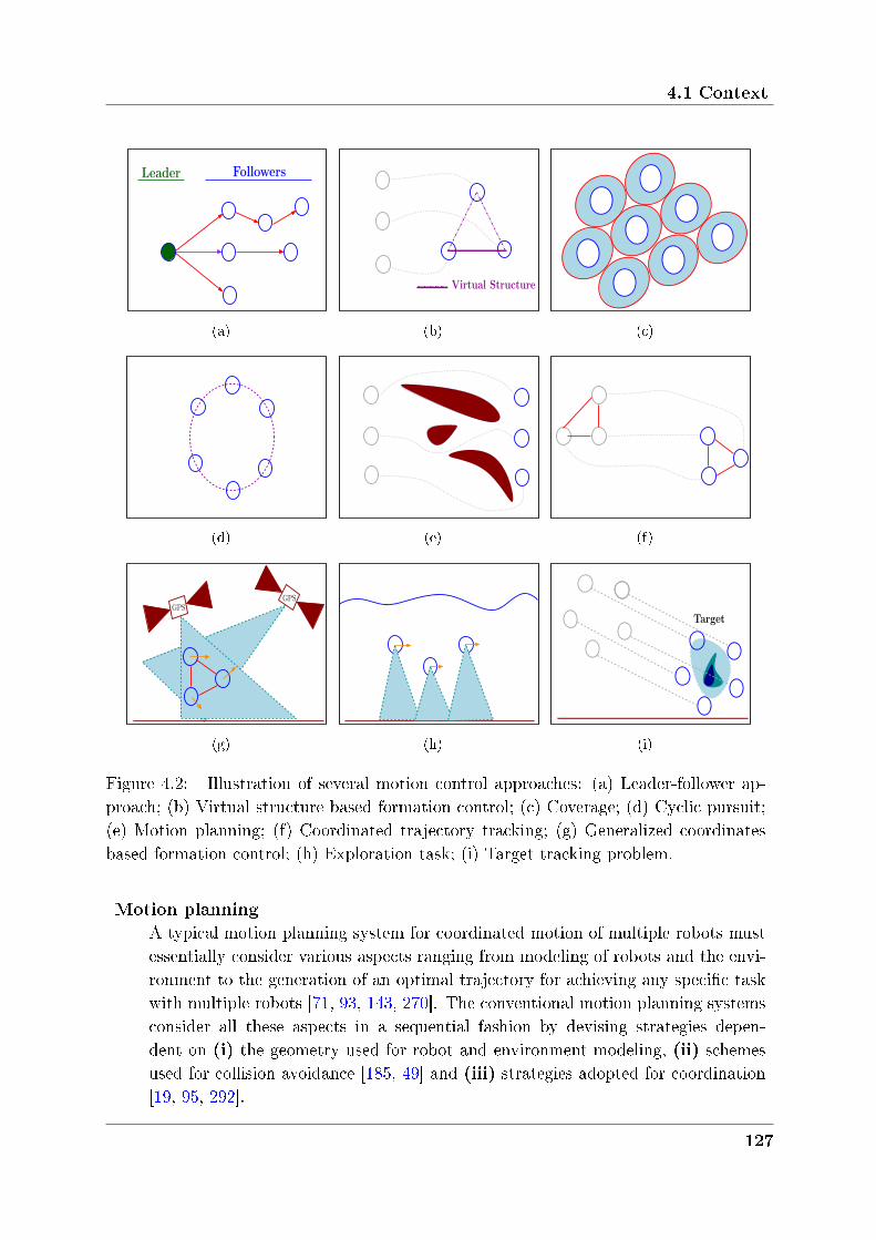
4.1 Context
Leader Followers
(a)
Virtual Structure
(b) (c)
(d) (e) (f)
GPSGPS
(g) (h)
Target
(i)
Figure 4.2: Illustration of several motion control approaches: (a) Leader-follower ap-proach; (b) Virtual structure based formation control; (c) Coverage; (d) Cyclic pursuit;(e) Motion planning; (f) Coordinated trajectory tracking; (g) Generalized coordinatesbased formation control; (h) Exploration task; (i) Target tracking problem.
Motion planning
A typical motion planning system for coordinated motion of multiple robots mustessentially consider various aspects ranging from modeling of robots and the envi-ronment to the generation of an optimal trajectory for achieving any specic taskwith multiple robots [71, 93, 143, 270]. The conventional motion planning systemsconsider all these aspects in a sequential fashion by devising strategies depen-dent on (i) the geometry used for robot and environment modeling, (ii) schemesused for collision avoidance [185, 49] and (iii) strategies adopted for coordination[19, 95, 292].
127
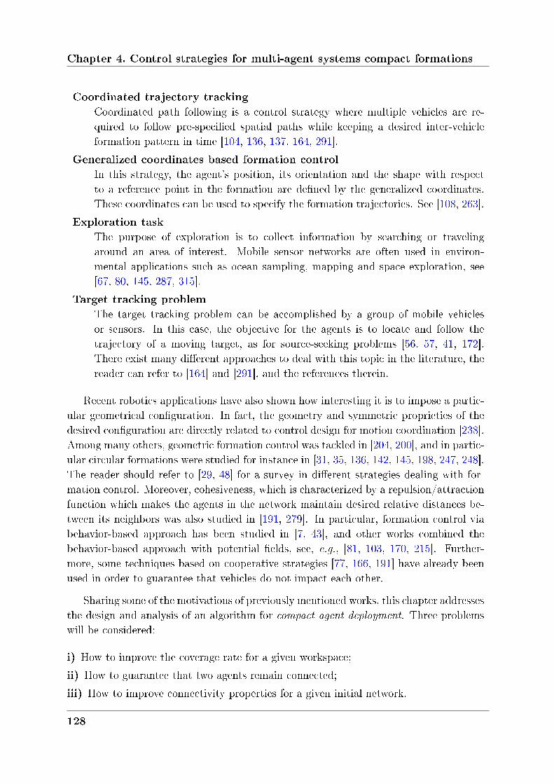
Chapter 4. Control strategies for multi-agent systems compact formations
Coordinated trajectory tracking
Coordinated path following is a control strategy where multiple vehicles are re-quired to follow pre-specied spatial paths while keeping a desired inter-vehicleformation pattern in time [104, 136, 137, 164, 291].
Generalized coordinates based formation control
In this strategy, the agent's position, its orientation and the shape with respectto a reference point in the formation are dened by the generalized coordinates.These coordinates can be used to specify the formation trajectories. See [108, 263].
Exploration task
The purpose of exploration is to collect information by searching or travelingaround an area of interest. Mobile sensor networks are often used in environ-mental applications such as ocean sampling, mapping and space exploration, see[67, 80, 145, 287, 315].
Target tracking problem
The target tracking problem can be accomplished by a group of mobile vehiclesor sensors. In this case, the objective for the agents is to locate and follow thetrajectory of a moving target, as for source-seeking problems [56, 57, 41, 172].There exist many dierent approaches to deal with this topic in the literature, thereader can refer to [164] and [291], and the references therein.
Recent robotics applications have also shown how interesting it is to impose a partic-ular geometrical conguration. In fact, the geometry and symmetric proprieties of thedesired conguration are directly related to control design for motion coordination [238].Among many others, geometric formation control was tackled in [204, 200], and in partic-ular circular formations were studied for instance in [31, 35, 136, 142, 145, 198, 247, 248].The reader should refer to [29, 48] for a survey in dierent strategies dealing with for-mation control. Moreover, cohesiveness, which is characterized by a repulsion/attractionfunction which makes the agents in the network maintain desired relative distances be-tween its neighbors was also studied in [191, 279]. In particular, formation control viabehavior-based approach has been studied in [7, 43], and other works combined thebehavior-based approach with potential elds, see, e.g., [81, 103, 170, 215]. Further-more, some techniques based on cooperative strategies [77, 166, 191] have already beenused in order to guarantee that vehicles do not impact each other.
Sharing some of the motivations of previously mentioned works, this chapter addressesthe design and analysis of an algorithm for compact agent deployment. Three problemswill be considered:
i) How to improve the coverage rate for a given workspace;
ii) How to guarantee that two agents remain connected;
iii) How to improve connectivity properties for a given initial network.
128
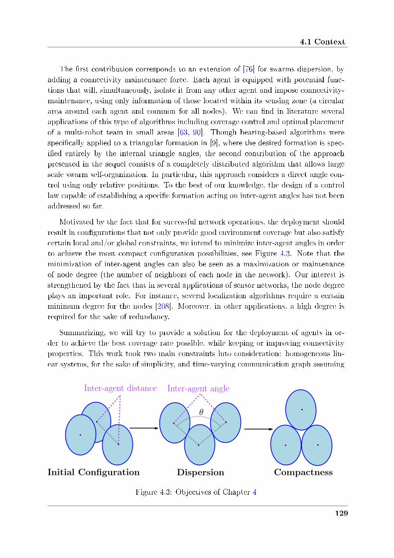
4.1 Context
The rst contribution corresponds to an extension of [76] for swarms dispersion, byadding a connectivity maintenance force. Each agent is equipped with potential func-tions that will, simultaneously, isolate it from any other agent and impose connectivity-maintenance, using only information of those located within its sensing zone (a circulararea around each agent and common for all nodes). We can nd in literature severalapplications of this type of algorithms including coverage control and optimal placementof a multi-robot team in small areas [63, 90]. Though bearing-based algorithms werespecically applied to a triangular formation in [9], where the desired formation is spec-ied entirely by the internal triangle angles, the second contribution of the approachpresented in the sequel consists of a completely distributed algorithm that allows largescale swarm self-organization. In particular, this approach considers a direct angle con-trol using only relative positions. To the best of our knowledge, the design of a controllaw capable of establishing a specic formation acting on inter-agent angles has not beenaddressed so far.
Motivated by the fact that for successful network operations, the deployment shouldresult in congurations that not only provide good environment coverage but also satisfycertain local and/or global constraints, we intend to minimize inter-agent angles in orderto achieve the most compact conguration possibilities, see Figure 4.3. Note that theminimization of inter-agent angles can also be seen as a maximization or maintenanceof node degree (the number of neighbors of each node in the network). Our interest isstrengthened by the fact that in several applications of sensor networks, the node degreeplays an important role. For instance, several localization algorithms require a certainminimum degree for the nodes [208]. Moreover, in other applications, a high degree isrequired for the sake of redundancy.
Summarizing, we will try to provide a solution for the deployment of agents in or-der to achieve the best coverage rate possible, while keeping or improving connectivityproperties. This work took two main constraints into consideration: homogeneous lin-ear systems, for the sake of simplicity, and time-varying communication graph assuming
Initial Configuration CompactnessDispersion
θ
Inter-agent angleInter-agent distance
Figure 4.3: Objectives of Chapter 4
129
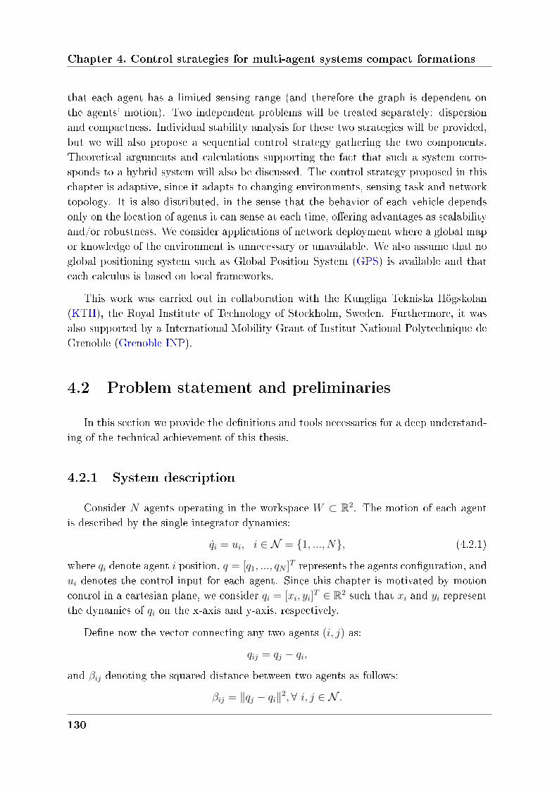
Chapter 4. Control strategies for multi-agent systems compact formations
that each agent has a limited sensing range (and therefore the graph is dependent onthe agents' motion). Two independent problems will be treated separately: dispersionand compactness. Individual stability analysis for these two strategies will be provided,but we will also propose a sequential control strategy gathering the two components.Theoretical arguments and calculations supporting the fact that such a system corre-sponds to a hybrid system will also be discussed. The control strategy proposed in thischapter is adaptive, since it adapts to changing environments, sensing task and networktopology. It is also distributed, in the sense that the behavior of each vehicle dependsonly on the location of agents it can sense at each time, oering advantages as scalabilityand/or robustness. We consider applications of network deployment where a global mapor knowledge of the environment is unnecessary or unavailable. We also assume that noglobal positioning system such as Global Position System (GPS) is available and thateach calculus is based on local frameworks.
This work was carried out in collaboration with the Kungliga Tekniska Högskolan(KTH), the Royal Institute of Technology of Stockholm, Sweden. Furthermore, it wasalso supported by a International Mobility Grant of Institut National Polytechnique deGrenoble (Grenoble INP).
4.2 Problem statement and preliminaries
In this section we provide the denitions and tools necessaries for a deep understand-ing of the technical achievement of this thesis.
4.2.1 System description
Consider 𝑁 agents operating in the workspace 𝑊 ⊂ R2. The motion of each agentis described by the single integrator dynamics:
𝑞𝑖 = 𝑢𝑖, 𝑖 ∈ 𝒩 = 1, ..., 𝑁, (4.2.1)
where 𝑞𝑖 denote agent 𝑖 position, 𝑞 = [𝑞1, ..., 𝑞𝑁 ]𝑇 represents the agents conguration, and𝑢𝑖 denotes the control input for each agent. Since this chapter is motivated by motioncontrol in a cartesian plane, we consider 𝑞𝑖 = [𝑥𝑖, 𝑦𝑖]
𝑇 ∈ R2 such that 𝑥𝑖 and 𝑦𝑖 representthe dynamics of 𝑞𝑖 on the x-axis and y-axis, respectively.
Dene now the vector connecting any two agents (𝑖, 𝑗) as:
𝑞𝑖𝑗 = 𝑞𝑗 − 𝑞𝑖,
and 𝛽𝑖𝑗 denoting the squared distance between two agents as follows:
𝛽𝑖𝑗 = ‖𝑞𝑗 − 𝑞𝑖‖2, ∀ 𝑖, 𝑗 ∈ 𝒩 .
130
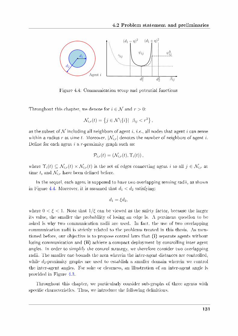
4.2 Problem statement and preliminaries
γij
βijd21
(d1 − η)2 (d1 + η)2
ψijd1
Agent id22
ψhijd1
d2
Figure 4.4: Communication setup and potential functions
Throughout this chapter, we denote for 𝑖 ∈ 𝒩 and 𝑟 > 0:
𝒩𝑖,𝑟(𝑡) =𝑗 ∈ 𝒩∖𝑖| 𝛽𝑖𝑗 < 𝑟2
,
as the subset of 𝒩 including all neighbors of agent 𝑖, i.e., all nodes that agent 𝑖 can sensewithin a radius 𝑟 at time 𝑡. Moreover, |𝒩𝑖,𝑟| denotes the number of neighbors of agent 𝑖.Dene for each agent 𝑖 a 𝑟-proximity graph such as:
𝒫𝑖,𝑟(𝑡) = (𝒩𝑖,𝑟(𝑡),Υ𝑖(𝑡)) ,
where Υ𝑖(𝑡) ⊆ 𝒩𝑖,𝑟(𝑡) × 𝒩𝑖,𝑟(𝑡) is the set of edges connecting agent 𝑖 to all 𝑗 ∈ 𝒩𝑖,𝑟 attime 𝑡, and 𝒩𝑖,𝑟 have been dened before.
In the sequel, each agent is supposed to have two overlapping sensing radii, as shownin Figure 4.4. Moreover, it is assumed that 𝑑1 < 𝑑2 satisfying:
𝑑1 = 𝜉𝑑2,
where 0 < 𝜉 < 1. Note that 1/𝜉 can be viewed as the safety factor, because the largerits value, the smaller the probability of losing an edge is. A pertinent question to beasked is why two communication radii are used. In fact, the use of two overlappingcommunication radii is strictly related to the problems treated in this thesis. As men-tioned before, our objective is to propose control laws that (i) separate agents withoutlosing communication and (ii) achieve a compact deployment by controlling inter-agentangles. In order to simplify the control strategy, we therefore consider two overlappingradii. The smaller one bounds the area wherein the inter-agent distances are controlled,while 𝑑2-proximity graphs are used to establish a smaller domain wherein we controlthe inter-agent angles. For sake or clearness, an illustration of an inter-agent angle isprovided in Figure 4.3.
Throughout this chapter, we particularly consider sub-graphs of three agents withspecic characteristics. Thus, we introduce the following denitions.
131
Chapter 4. Control strategies for multi-agent systems compact formations
Definition 4.1. A triplet (𝑖, 𝑗, 𝑘) ∈ 𝒩 3 is a Triangle if 𝑖, 𝑗, 𝑘 are all distinct and
𝑖, 𝑘 ∈ 𝒩𝑗,𝑑2 , 𝑖 /∈ 𝒩𝑘,𝑑2 .
Thus, a Triangle is a connected graph. Moreover, the central vertex can sense theother two agents, while the other two can only sense the central agent. Note that, interms of notation, the order of agents matters. This means that, when Triangles arediscussed, a triplet (𝑖, 𝑗, 𝑘) is centered at 𝑗.
Definition 4.2. A triplet (𝑖, 𝑗, 𝑘) ∈ 𝒩 3 is a Compact Triangle if 𝑖, 𝑗, 𝑘 are all distinct
and
𝑖, 𝑘 ∈ 𝒩𝑗,𝑑2 , 𝑖 ∈ 𝒩𝑘,𝑑2 .
Then, it follows that a Compact Triangle is a three nodes complete graph. Alsothroughout this chapter, for each Triangle (𝑖, 𝑗, 𝑘), we will often use the term "inter-agentangle", illustrated in Figure 4.3, to indicate the angle formed by these three agents suchthat:
𝜃𝑖𝑗𝑘 = arccos(<𝑞𝑗𝑖,𝑞𝑗𝑘>
‖𝑞𝑖𝑗‖·‖𝑞𝑗𝑘‖
). (4.2.2)
To minimize angles, we intend to apply to each triangle formed of three agents, aforce proportional to the dierence between the angle value and the reference. Thisforce lies down on a perpendicular direction of 𝑞𝑖𝑗, denoted 𝑞⊥𝑖𝑗 . Since we intend toachieve compact formations composed of equilateral triangles, this inherently means weare aiming for each angle to be equal to 𝜋
3. Therefore, this value will be taken as reference.
In this chapter, we are going to analyze a dispersion and compactness control laws,individually, and nally a sequential controller. For the dispersion algorithm, we denethe set of feasible initial conditions:
ℐ(𝑑1) =𝑞 ∈ 𝑊 | ∀𝑖 ∈ 𝒩 , 𝑗 ∈ 𝒩𝑖,𝑑2 , 𝛽𝑖𝑗 ∈ ]0, 𝑑21]
,
and the set of desired nal congurations as:
ℱ(𝑑1, 𝜂) =𝑞 ∈ 𝑊 | ∀𝑖 ∈ 𝒩 , 𝑗 ∈ 𝒩𝑖,𝑑2 , (𝑑1 − 𝜂)2 < 𝛽𝑖𝑗 < (𝑑1 + 𝜂)2
.
Dene the set including all congurations where each agent has at most ∆ neighborsin 𝑑2-proximity graph as:
𝒟(𝑑2,∆) = 𝑞 ∈ 𝑊 | ∀𝑖 ∈ 𝒩 , |𝒩𝑖,𝑑2| ≤ ∆ .
Note that ∆ is a positive integer value to be dened. Dene now:
ℰ(𝑑1) =𝑞 ∈ 𝑊 | for all Triangles (𝑖, 𝑗, 𝑘), 𝛽𝑖𝑗 = 𝛽𝑗𝑘 = 𝑑21
,
132

4.2 Problem statement and preliminaries
as the set including the congurations where all Triangles have two equal edges of length𝑑1. Thus, for the compactness control strategy, we dene the set of feasible initialconditions as:
ℱ ′(𝑑1, 𝑑2) = 𝒟(𝑑2, 2) ∩ ℰ(𝑑1).
This means that we assume formations where each agent has at most two neighborsand where the length of the existing edges is constant and equal to 𝑑1. It is importantto point out that this assumption includes, among many others, the ring formation.More precisely, this particular conguration can be represented by a graph where eachagent has exactly two neighbors. Consequently, it follows from a geometrical point ofview that the control strategy presented in this article is not suited for such a problem.In particular, due to the perfect balanced forces applied to each agent, an inter-agentangle based controller is unable to solve the compact formation problem. Therefore, thisspecial formation is excluded from the following discussion.
Since the objective is to achieve the most compact conguration possible, we candene a set of desired congurations such that:
𝒢(𝑑1, 𝑑2) =𝑞 ∈ 𝑊 |∀𝑗 ∈ 𝒩 ,∃(𝑖, 𝑘) ∈ 𝒩 2
𝑗,𝑑2st. 𝛽𝑖𝑗 = 𝛽𝑗𝑘 = 𝛽𝑘𝑖 = 𝑑21
.
As a consequence, this triplet (𝑖, 𝑗, 𝑘) is a Compact Triangle.
4.2.2 Definition of the potential functions
From the control theory point of view, cohesiveness is characterized by a repul-sion/attraction function which makes the agents in the network maintain desired relativedistances between its neighbors, see, e.g., [191, 279]. In particular, formation control viabehavior-based approach have been studied in [7, 43], and others works combined thebehavior-based approach with potential elds as in, for example, [81, 103, 170, 215].More precisely, in [215] group formation behavior is based on social potential elds andarticial potential trenches are used to represent the formation trajectory of the groupin [103]. Moreover, some techniques based on cooperative strategies have already beenused in order to guarantee that vehicles do not impact each other [77, 166, 191]. Forinstance, the authors of [170] apply this method to a non-linear dynamic system for ob-stacle avoidance and trajectory generation. The reader should refer to [48] for a surveyin dierent strategies dealing with formation control.
Our deployment algorithm is based on articial potential elds. In the sequel, aspecial attention is paid to the inverse agreement protocols presented in [76], amongmany other works in this eld. In [76], authors showed that the closed loop systemreaches a conguration in which the minimum distance between any pair of agents islarger than a specic lower bound. Moreover, it was proven [76] that this lower bound
133
Chapter 4. Control strategies for multi-agent systems compact formations
coincides with the agents' sensing radius. Based on this, our contribution consists on anextension of this work by adding a connectivity maintenance component. In Figure 4.4,we can see the two potential functions, 𝛾𝑖𝑗 and 𝜓𝑖𝑗 ∈ 𝐶([0,+∞)), whose argument is 𝛽𝑖𝑗(dened before).
These two functions are designed with the key features described for all 𝑖, 𝑗 ∈ 𝒩 and𝑖 = 𝑗 as follows:
Definition of the potential function 𝛾𝑖𝑗 for a couple of distinct agents (𝑖, 𝑗) ∈ 𝒩 2:
∙ 𝛾𝑖𝑗 is a decreasing function, twice continuously dierentiable;∙ 𝛾𝑖𝑗 tends to +∞ when 𝛽𝑖𝑗 tends to zero;∙ 𝜕𝛾𝑖𝑗
𝜕𝛽𝑖𝑗= 0 if 𝛽𝑖𝑗 ≥ 𝑑21.
Definition of the potential function 𝜓𝑖𝑗 for a couple of distinct agents (𝑖, 𝑗) ∈ 𝒩 2:
∙ 𝜓𝑖𝑗 tends to ∞ when 𝛽𝑖𝑗 tends to (𝑑1 ± 𝜂)2;∙ 𝜓𝑖𝑗 = 𝛾𝑖𝑗 and
𝜕𝛾𝑖𝑗𝜕𝛽𝑖𝑗
= 0 if 𝛽𝑖𝑗 = 𝑑21.
where 𝜂 is a positive scalar dening the size of the desired neighborhood for con-nectivity maintenance.
Using this framework, one has not taken into account dynamical graphs, where newedges are added, i.e., when two agents come close enough to sense each other but did notform an edge before. This scenario should also be considered here. Indeed, it is possiblethat, as a consequence of the second stage, agents will get new neighbors as time evolves.Dene:
𝒩 ℎ𝑖,𝑑1+𝜂
=𝑗 ∈ 𝒩∖𝑖, 𝛽𝑖𝑗 < (𝑑1 + 𝜂)2, 𝑖𝑗 < 0
,
as the subset of the sensing zone of agent 𝑖 including all agents that form a new edgewith agent 𝑖. In order to ensure a smooth transition to 𝜓𝑖𝑗, we dene 𝜓ℎ𝑖𝑗 such that:
Additional features of the potential function 𝜓ℎ𝑖𝑗:
∙ 𝜓ℎ𝑖𝑗 is dierentiable everywhere;
∙ 𝜓ℎ𝑖𝑗 = 𝜓𝑖𝑗 and𝜕𝜓ℎ
𝑖𝑗
𝜕𝛽𝑖𝑗=
𝜕𝜓𝑖𝑗
𝜕𝛽𝑖𝑗when 𝛽𝑖𝑗 ≤ 𝑑21;
∙ 𝜓ℎ𝑖𝑗 is strictly increasing when 𝑑21 < 𝛽𝑖𝑗 < (𝑑1 + 𝜂)2;∙ 𝜓ℎ𝑖𝑗 is constant when 𝛽𝑖𝑗 > (𝑑1 + 𝜂)2.
We have introduced here the considered model as well as the potential elds neededfor the design of the dispersion controller. This algorithm will now be treated in thefollowing section.
134
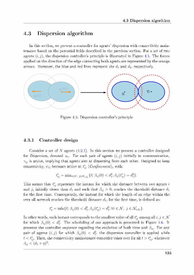
4.3 Dispersion algorithm
4.3 Dispersion algorithm
In this section, we present a controller for agents' dispersion with connectivity main-tenance based on the potential elds described in the previous section. For a set of twoagents (𝑖, 𝑗), the dispersion controller's principle is illustrated in Figure 4.5. The forcesapplied on the direction of the edge connecting both agents are represented by the orangearrows. Moreover, the blue and red lines represent the 𝑑1 and 𝑑2, respectively.
qi(0)qjqi
qj(0)
Figure 4.5: Dispersion controller's principle
4.3.1 Controller design
Consider a set of 𝑁 agents (4.2.1). In this section we present a controller designedfor Dispersion, denoted 𝑢1. For each pair of agents (𝑖, 𝑗) initially in communication,𝛾𝑖𝑗 is active, implying that agents aim at dispersing from each other. Designed to keepconnectivity, 𝜓𝑖𝑗 becomes active at 𝑡*𝑖𝑗 (Confinement), with:
𝑡*𝑖𝑗 = min𝑖∈𝒩 , 𝑗∈𝒩𝑖,𝑑1𝑡| 𝛽𝑖𝑗(0) < 𝑑21, 𝛽𝑖𝑗(𝑡
*𝑖𝑗) = 𝑑21.
This means that 𝑡*𝑖𝑗 represents the instant for which the distance between two agents 𝑖and 𝑗, initially closer than 𝑑1 and such that 𝑖𝑗 > 0, reaches the threshold distance 𝑑1for the rst time. Consequently, the instant for which the length of an edge within theover all network reaches the threshold distance 𝑑1, for the rst time, is dened as:
𝑡*𝑎 = min𝑡| 𝛽𝑖𝑗(0) < 𝑑21, 𝛽𝑖𝑗(𝑡*𝑖𝑗) = 𝑑21,∀𝑖 ∈ 𝒩 , 𝑗 ∈ 𝒩𝑖,𝑑1.
In other words, such instant corresponds to the smallest value of all 𝑡*𝑖𝑗 among all 𝑖, 𝑗 ∈ 𝒩for which 𝛽𝑖𝑗(0) < 𝑑21. The scheduling of our approach is presented in Figure 4.6. Itpresents the controller sequence regarding the evolution of both time and 𝛽𝑖𝑗. For anypair of agents (𝑖, 𝑗) for which 𝛽𝑖𝑗(0) < 𝑑21, the dispersion controller is applied while𝑡 < 𝑡*𝑖𝑗. Then, the connectivity maintenance controller takes over for all 𝑡 > 𝑡*𝑖𝑗, whenever𝛽𝑖𝑗 < (𝑑1 + 𝜂)2.
135
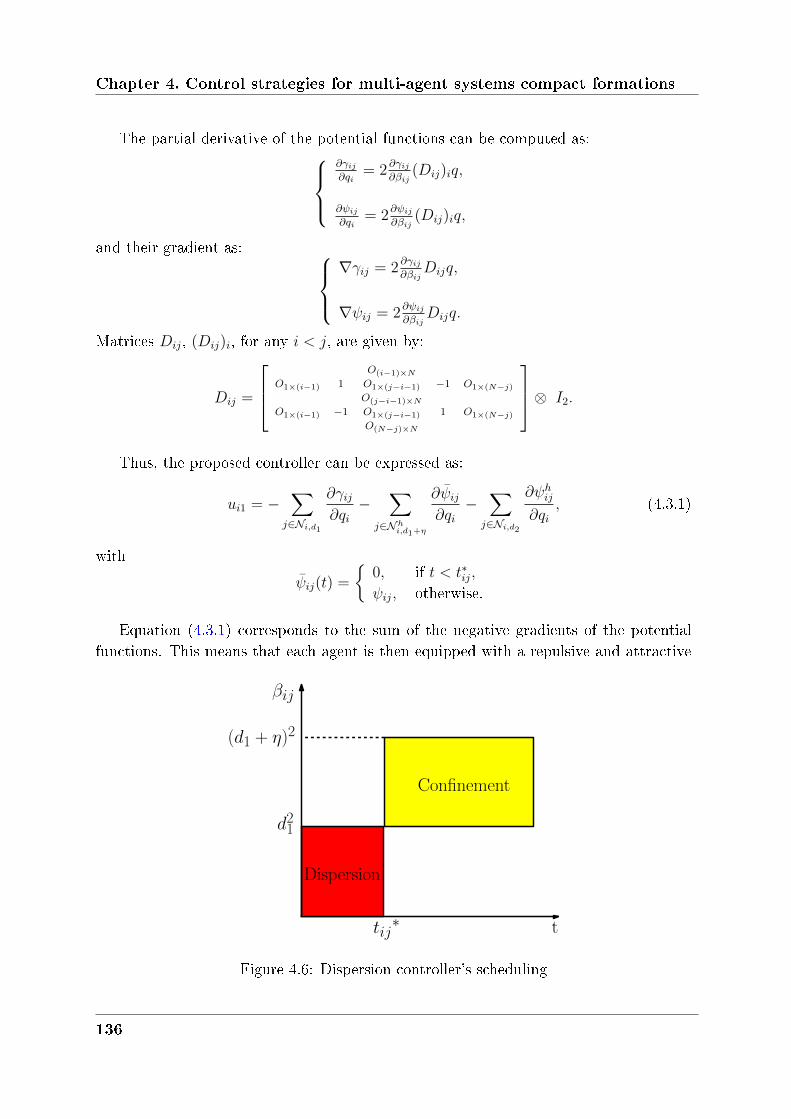
Chapter 4. Control strategies for multi-agent systems compact formations
The partial derivative of the potential functions can be computed as:⎧⎪⎨⎪⎩𝜕𝛾𝑖𝑗𝜕𝑞𝑖
= 2𝜕𝛾𝑖𝑗𝜕𝛽𝑖𝑗
(𝐷𝑖𝑗)𝑖𝑞,
𝜕𝜓𝑖𝑗
𝜕𝑞𝑖= 2
𝜕𝜓𝑖𝑗
𝜕𝛽𝑖𝑗(𝐷𝑖𝑗)𝑖𝑞,
and their gradient as: ⎧⎪⎨⎪⎩∇𝛾𝑖𝑗 = 2
𝜕𝛾𝑖𝑗𝜕𝛽𝑖𝑗
𝐷𝑖𝑗𝑞,
∇𝜓𝑖𝑗 = 2𝜕𝜓𝑖𝑗
𝜕𝛽𝑖𝑗𝐷𝑖𝑗𝑞.
Matrices 𝐷𝑖𝑗, (𝐷𝑖𝑗)𝑖, for any 𝑖 < 𝑗, are given by:
𝐷𝑖𝑗 =
⎡⎢⎣𝑂(𝑖−1)×𝑁
𝑂1×(𝑖−1) 1 𝑂1×(𝑗−𝑖−1) −1 𝑂1×(𝑁−𝑗)
𝑂(𝑗−𝑖−1)×𝑁
𝑂1×(𝑖−1) −1 𝑂1×(𝑗−𝑖−1) 1 𝑂1×(𝑁−𝑗)
𝑂(𝑁−𝑗)×𝑁
⎤⎥⎦⊗ 𝐼2.
Thus, the proposed controller can be expressed as:
𝑢𝑖1 = −∑
𝑗∈𝒩𝑖,𝑑1
𝜕𝛾𝑖𝑗𝜕𝑞𝑖
−∑
𝑗∈𝒩ℎ𝑖,𝑑1+𝜂
𝜕𝜓𝑖𝑗𝜕𝑞𝑖
−∑
𝑗∈𝒩𝑖,𝑑2
𝜕𝜓ℎ𝑖𝑗𝜕𝑞𝑖
, (4.3.1)
with
𝜓𝑖𝑗(𝑡) =
0, if 𝑡 < 𝑡*𝑖𝑗,
𝜓𝑖𝑗, otherwise.
Equation (4.3.1) corresponds to the sum of the negative gradients of the potentialfunctions. This means that each agent is then equipped with a repulsive and attractive
Dispersion
Confinement
tij∗ t
Confinement
βij
d21
(d1 + η)2
Figure 4.6: Dispersion controller's scheduling
136
4.3 Dispersion algorithm
eld with respect to another agent within its sensing zone. As mentioned before, in orderto take into account newly formed edges, consider 𝜓𝐻𝑖𝑗 as a modied potential functionbased on 𝜓𝑖𝑗 and 𝜓ℎ𝑖𝑗, such that:
𝜓𝐻𝑖𝑗 =
𝜓ℎ𝑖𝑗, if 𝑗 ∈ 𝒩 ℎ
𝑖,𝑑1+𝜂,
𝜓𝑖𝑗, otherwise .
Whenever an agent 𝑗 forms a new edge with agent 𝑖, the function 𝜓𝐻𝑖𝑗 switches from𝜓ℎ𝑖𝑗 to 𝜓𝑖𝑗. Dene also:
𝜎𝐻𝑖𝑗 =
⎧⎪⎪⎨⎪⎪⎩𝜕𝜓ℎ
𝑖𝑗
𝜕𝛽𝑖𝑗, if 𝑗 ∈ 𝒩 ℎ
𝑖,𝑑1+𝜂,
𝜕𝜓𝑖𝑗
𝜕𝛽𝑖𝑗, otherwise .
Thus, it yields:𝑢1 = −2 [𝑅1 ⊗ 𝐼2 +𝑅2 ⊗ 𝐼2] 𝑞, (4.3.2)
where 𝑅1 and 𝑅2 are 𝑁 ×𝑁 matrices dened as follows:
(𝑅1)𝑝𝑞 =
⎧⎪⎪⎪⎨⎪⎪⎪⎩∑
𝑗∈𝒩∖𝑝
𝜕𝛾𝑝𝑗𝜕𝛽𝑝𝑗
, if 𝑝 = 𝑞,
− 𝜕𝛾𝑝𝑞𝜕𝛽𝑝𝑞
, otherwise.
(𝑅2)𝑝𝑞 =
⎧⎪⎨⎪⎩∑
𝑗∈𝒩∖𝑝
𝜎𝐻𝑝𝑗, if 𝑝 = 𝑞,
− 𝜎𝐻𝑝𝑞, otherwise.
The proposed controller for agent's dispersion is expressed in (4.3.2). The followingsection will provide stability conditions and performance analysis.
4.3.2 Stability analysis
This section provides a theoretical stability analysis for the dispersion algorithm. Therespective controller ensures dispersion of all agents in the workspace, while maintainingconnectivity and avoiding loosing edges. The next theorem states our results.
Theorem 4.1. (Rodrigues de Campos et al. [229]) Consider 𝑁 agents (4.2.1) drivenby the control law (4.3.1). Assume a set of feasible initial conditions ℐ(𝑑1). Then the
system reaches a final static configuration belonging to ℱ(𝑑1, 𝜂).
Proof. Consider 𝑉𝑑 as a Lyapunov function such that:
𝑉𝑑(𝑞) =∑𝑖∈𝒩
∑𝑗∈𝒩∖𝑖
[𝛾𝑖𝑗(𝛽𝑖𝑗) + 𝜓𝐻𝑖𝑗 (𝛽𝑖𝑗)
]. (4.3.3)
137
Chapter 4. Control strategies for multi-agent systems compact formations
For the sake of readability, the argument of the Lyapunov function will be omitted.We can compute: ⎧⎪⎨⎪⎩
∇𝛾𝑖𝑗 = 2𝜕𝛾𝑖𝑗𝜕𝛽𝑖𝑗
(𝑞𝑖 − 𝑞𝑗),
∇𝜓ℎ𝑖𝑗 = 2𝜕𝜓ℎ
𝑖𝑗
𝜕𝛽𝑖𝑗(𝑞𝑖 − 𝑞𝑗),
and𝜕𝛾𝑖𝑗𝜕𝛽𝑖𝑗
=𝜕𝛾𝑗𝑖𝜕𝛽𝑗𝑖
,𝜕𝜓𝑖𝑗𝜕𝛽𝑖𝑗
=𝜕𝜓𝑗𝑖𝜕𝛽𝑗𝑖
, 𝜎𝐻𝑖𝑗 = 𝜎𝐻𝑗𝑖 ,
due to symmetry. Thus, it follows that:
∇𝑉𝑑 =∑𝑖∈𝒩
∑𝑗∈𝒩∖𝑖
[∇𝛾𝑖𝑗 + ∇𝜓𝐻𝑖𝑗
]= 4(𝑅1 ⊗ 𝐼2)𝑞 + 4(𝑅2 ⊗ 𝐼2)𝑞 = 4 [(𝑅1 +𝑅2) ⊗ 𝐼2] 𝑞.
Finally, the derivative of the Lyapunov function can be expressed as:
𝑑 = (∇𝑉𝑑)𝑇 𝑞 = −8‖[(𝑅1 ⊗ 𝐼2) + (𝑅2 ⊗ 𝐼2)]𝑞‖2. (4.3.4)
Therefore, 𝑑 is strictly negative for all 𝑡 > 0, guaranteeing the system's convergence.Let us discuss this conclusion. Consider any 𝑡 < 𝑡*𝑎. For any two agents initially closesuch that 𝛽𝑖𝑗(0) < 𝑑21,∀𝑗 ∈ 𝒩𝑖,𝑑1 , we have 𝜕𝛾𝑖𝑗
𝜕𝛽𝑖𝑗< 0 if 𝛽𝑖𝑗 < 𝑑21. Moreover, 𝜕𝛾𝑖𝑗
𝜕𝛽𝑖𝑗= 0 if
𝛽𝑖𝑗 ≥ 𝑑21, and therefore 𝛽𝑖𝑗 = 𝑑21 corresponds to the equilibrium point of 𝛾𝑖𝑗. Since thecontribution of the remaining potential elds is null for 𝛽𝑖𝑗 < 𝑑21, it follows that for anytwo agents 𝑖𝑗 > 0 such that 𝛽𝑖𝑗 will eventually reach a close neighborhood of 𝑑21. At𝑡 = 𝑡*𝑎, the potential function 𝜓𝑖𝑗 is activated for at least one pair of agents. For this pairof agents, two evolution cases are possible: either 𝑖𝑗 < 0 such that (𝑑1 − 𝜂)2 < 𝛽𝑖𝑗 < 𝑑21(situation (i)), or 𝑖𝑗 > 0 such that 𝑑21 < 𝛽𝑖𝑗 < (𝑑1 + 𝜂)2, (situation (ii)):
(i) By denition, if (𝑑1−𝜂)2 < 𝛽𝑖𝑗 < 𝑑21, the quantities𝜕𝛾𝑖𝑗𝜕𝛽𝑖𝑗
and 𝜕𝜓𝑖𝑗
𝜕𝛽𝑖𝑗are strictly negative.
This means that throughout (4.3.1) a repulsive force is applied to agents 𝑖 and 𝑗,and consequently 𝛽𝑖𝑗 will increase such that 𝑖𝑗 > 0. Moreover, since 𝑉𝑑 tends to+∞ whenever 𝛽𝑖𝑗 tends to (𝑑1 − 𝜂)2, we can conclude that the distance separatingagents will never reach (𝑑1 − 𝜂)2.
(ii) By denition, if 𝑑21 < 𝛽𝑖𝑗 < (𝑑1 + 𝜂)2, the quantities 𝜕𝛾𝑖𝑗𝜕𝛽𝑖𝑗
and 𝜕𝜓𝑖𝑗
𝜕𝛽𝑖𝑗are equal to zero
and strictly positive, respectively. This means that throughout (4.3.1) a attractiveforce is applied to agents 𝑖 and 𝑗 and therefore 𝛽𝑖𝑗 will decrease such that 𝑖𝑗 < 0.Since 𝑉𝑑 tends to ∞ when 𝛽𝑖𝑗 tend to (𝑑1 + 𝜂)2, we can conclude that the distanceseparating agents will never reach (𝑑1 + 𝜂)2.
Considering the specic design characteristics of 𝜓𝐻𝑖𝑗 , it follows that if a new edge iscreated, i.e., if the distance separating agents 𝑖 and 𝑗 is lower than a certain threshold𝑑1 + 𝜂, the transition between 𝜓ℎ𝑖𝑗 and 𝜓𝑖𝑗 is held in a suciently smooth manner. This
138
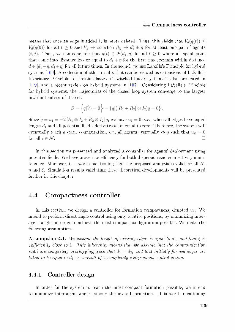
4.4 Compactness controller
means that once an edge is added it is never deleted. Thus, this yields that 𝑉𝑑(𝑞(𝑡)) ≤𝑉𝑑(𝑞(0)) for all 𝑡 ≥ 0 and 𝑉𝑑 → ∞ when 𝛽𝑖𝑗 → 𝑑21 ± 𝜂 for at least one par of agents(𝑖, 𝑗). Then, we can conclude that 𝑞(𝑡) ∈ ℱ(𝑑1, 𝜂) for all 𝑡 ≥ 0 where all agent pairsthat come into distance less or equal to 𝑑1 + 𝜂 for the rst time, remain within distance𝑑 ∈ [𝑑1−𝜂, 𝑑1+𝜂] for all future times. In the sequel, we use LaSalle's Principle for hybridsystems [160]. A collection of other results that can be viewed as extensions of LaSalle'sInvariance Principle to certain classes of switched linear systems is also presented in[119], and a recent review on hybrid systems in [107]. Considering LaSalle's Principlefor hybrid systems, the trajectories of the closed loop system converge to the largestinvariant subset of the set:
𝑆 =𝑞|𝑑 = 0
= 𝑞|([𝑅1 +𝑅2] ⊗ 𝐼2)𝑞 = 0 .
Since 𝑞 = 𝑢1 = −2 [𝑅1 ⊗ 𝐼2 +𝑅2 ⊗ 𝐼2] 𝑞, we have 𝑢1 = 0, i.e., when all edges have equallength 𝑑1 and all potential eld's derivatives are equal to zero. Therefore, the system willeventually reach a static conguration, i.e., all agents eventually stop such that 𝑢𝑖1 = 0
for all 𝑖 ∈ 𝒩 .
In this section we presented and analyzed a controller for agents' deployment usingpotential elds. We have proven its eciency for both dispersion and connectivity main-tenance. Moreover, it is worth mentioning that the proposed analysis is valid for all 𝑁 ,𝜂 and 𝜉. Simulation results validating these theoretical developments will be presentedfurther in this chapter.
4.4 Compactness controller
In this section, we design a controller for formation compactness, denoted 𝑢2. Weintend to preform direct angle control using only relative positions, by minimizing inter-agent angles in order to achieve the most compact conguration possible. We make thefollowing assumption.
Assumption 4.1. We assume the length of existing edges is equal to 𝑑1, and that 𝜉 is
sufficiently close to 1. This inherently means that we assume that the communication
radii are completely overlapping, such that 𝑑1 = 𝑑2, and that initially formed edges are
taken to be equal to 𝑑1 as a result of a completely independent control action.
4.4.1 Controller design
In order for the system to reach the most compact formation possible, we intendto minimize inter-agent angles among the overall formation. It is worth mentioning
139
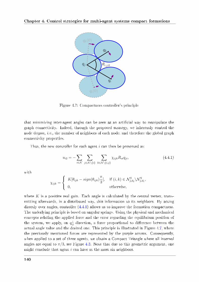
Chapter 4. Control strategies for multi-agent systems compact formations
qj
qk(0)
qi(0)
θi,j,k
qk
qi
Figure 4.7: Compactness controller's principle
that minimizing inter-agent angles can be seen as an articial way to manipulate thegraph connectivity. Indeed, through the proposed strategy, we inherently control thenode degree, i.e., the number of neighbors of each node, and therefore the global graphconnectivity properties.
Thus, the new controller for each agent 𝑖 can then be presented as:
𝑢𝑖2 = −∑𝑖∈𝒩
∑𝑗∈𝒩∖𝑖
∑𝑘∈𝒩∖𝑖,𝑗
𝜒𝑖𝑗𝑘𝑅𝑜𝑡𝑞𝑗𝑖, (4.4.1)
with
𝜒𝑖𝑗𝑘 =
⎧⎨⎩ 𝐾[𝜃𝑖𝑗𝑘 − 𝑠𝑖𝑔𝑛(𝜃𝑖𝑗𝑘)𝜋
3], if (𝑖, 𝑘) ∈ 𝒩 2
𝑗,𝑑2∖𝒩 2
𝑗,𝑑1,
0, otherwise,
where 𝐾 is a positive real gain. Each angle is calculated by the central vertex, trans-mitting afterwards, in a distributed way, this information to its neighbors. By actingdirectly over angles, controller (4.4.1) allows us to improve the formation compactness.The underlying principle is based on angular springs. Using the physical and mechanicalconcepts relating the applied force and the error regarding the equilibrium position ofthe system, we apply, on 𝑞⊥𝑖𝑗 direction, a force proportional to dierence between theactual angle value and the desired one. This principle is illustrated in Figure 4.7, wherethe previously mentioned forces are represented by the purple arrows. Consequently,when applied to a set of three agents, we obtain a Compact Triangle where all internalangles are equal to 𝜋/3, see Figure 4.3. Note that due to this geometric argument, onemight conclude that agent 𝑖 can have at the most six neighbors.
140
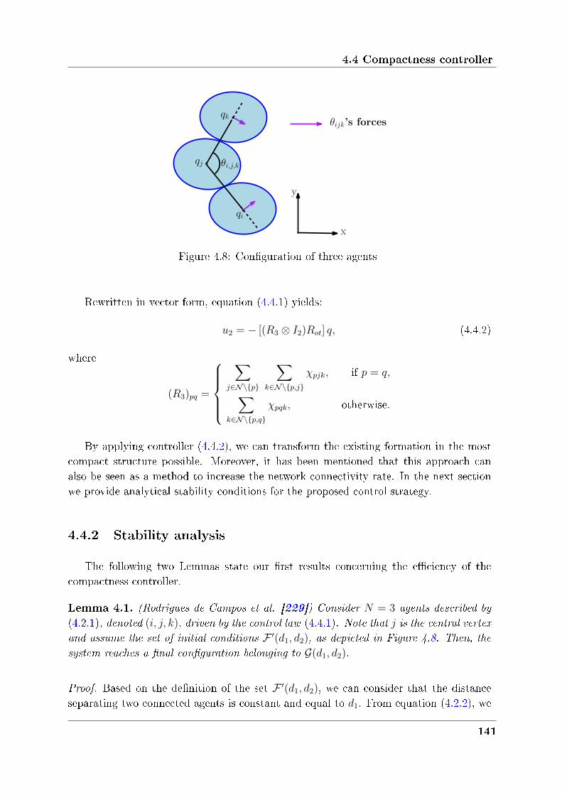
4.4 Compactness controller
qj
qk
qi
θi,j,k
y
x
θijk’s forces
Figure 4.8: Conguration of three agents
Rewritten in vector form, equation (4.4.1) yields:
𝑢2 = − [(𝑅3 ⊗ 𝐼2)𝑅𝑜𝑡] 𝑞, (4.4.2)
where
(𝑅3)𝑝𝑞 =
⎧⎪⎪⎪⎨⎪⎪⎪⎩∑
𝑗∈𝒩∖𝑝
∑𝑘∈𝒩∖𝑝,𝑗
𝜒𝑝𝑗𝑘, if 𝑝 = 𝑞,
∑𝑘∈𝒩∖𝑝,𝑞
𝜒𝑝𝑞𝑘, otherwise.
By applying controller (4.4.2), we can transform the existing formation in the mostcompact structure possible. Moreover, it has been mentioned that this approach canalso be seen as a method to increase the network connectivity rate. In the next sectionwe provide analytical stability conditions for the proposed control strategy.
4.4.2 Stability analysis
The following two Lemmas state our rst results concerning the eciency of thecompactness controller.
Lemma 4.1. (Rodrigues de Campos et al. [229]) Consider 𝑁 = 3 agents described by
(4.2.1), denoted (𝑖, 𝑗, 𝑘), driven by the control law (4.4.1). Note that 𝑗 is the central vertexand assume the set of initial conditions ℱ ′(𝑑1, 𝑑2), as depicted in Figure 4.8. Then, the
system reaches a final configuration belonging to 𝒢(𝑑1, 𝑑2).
Proof. Based on the denition of the set ℱ ′(𝑑1, 𝑑2), we can consider that the distanceseparating two connected agents is constant and equal to 𝑑1. From equation (4.2.2), we
141
Chapter 4. Control strategies for multi-agent systems compact formations
can compute:𝑑
𝑑𝑡cos(𝜃𝑖𝑗𝑘) =
[< ˙𝑞𝑗𝑖, 𝑞𝑗𝑘 > + < 𝑞𝑗𝑖, ˙𝑞𝑗𝑘 >]
‖𝑞𝑗𝑖‖ ‖𝑞𝑗𝑘‖. (4.4.3)
We can easily obtain:
< 𝑞𝑗𝑖, 𝑞𝑗𝑘⊥ >= −‖𝑞𝑗𝑖‖‖𝑞𝑗𝑘‖ sin(𝜃𝑖𝑗𝑘), < 𝑞𝑗𝑖
⊥, 𝑞𝑗𝑘 >= ‖𝑞𝑗𝑖‖‖𝑞𝑗𝑘‖ sin(𝜃𝑖𝑗𝑘).
Considering controller (4.4.1), (4.4.3) can be written as:
𝑑
𝑑𝑡cos(𝜃𝑖𝑗𝑘) = 2𝐾
(𝜃𝑖𝑗𝑘 − 𝑠𝑖𝑔𝑛(𝜃𝑖𝑗𝑘)
𝜋
3
)sin(𝜃𝑖𝑗𝑘).
Finally, for all 𝑠𝑖𝑛(𝜃𝑖𝑗𝑘) = 0 we have:
𝜃𝑖𝑗𝑘 = −2𝐾(𝜃𝑖𝑗𝑘 − 𝑠𝑖𝑔𝑛(𝜃𝑖𝑗𝑘)
𝜋
3
).
Note that previous manipulations exclude cases where |𝜃𝑖𝑗𝑘| = 𝑘𝜋, since if 𝑠𝑖𝑛(𝜃𝑖𝑗𝑘) =
0 then:𝜃𝑖𝑗𝑘 = 2𝐾
(𝜃𝑖𝑗𝑘 − 𝑠𝑖𝑔𝑛(𝜃𝑖𝑗𝑘)
𝜋
3
)sin(𝜃𝑖𝑗𝑘) = 0,
which corresponds to a particular equilibrium oering two possible trajectories. In thiswork, and for the sake of simplicity, we consider that 𝜃𝑖𝑗𝑘 = 0 [𝜋], i.e., 𝜃𝑖𝑗𝑘 = 𝑘𝜋.Consider now the following Lyapunov function candidate:
𝑉𝑐(𝑞) =∑𝑗∈𝒩
∑𝑖∈𝒩𝑗,𝑑2
∑𝑘∈𝒩𝑗,𝑑2
∖𝑖
(|𝜃𝑖𝑗𝑘| −
𝜋
3
)2
.
Note that for each Triangle, there is only one inter-agent angle to be controlled. Due tothe geometric constraints that ℱ ′(𝑑1, 𝑑2) implies, |𝜃𝑖𝑗𝑘| ≥ 𝜋/3,∀𝑗 ∈ 𝒩 , (𝑖, 𝑘) ∈ 𝒩 2
𝑗,𝑑2, 𝑖 =
𝑘 (since in a isosceles Triangle edges are at least of length 𝑑1). Thus, either 𝜋/3 ≤ 𝜃𝑖𝑗𝑘 < 𝜋
or −𝜋 < 𝜃𝑖𝑗𝑘 ≤ −𝜋/3, which leads us to a continuous function 𝑉𝑐(𝑞). Its derivative canthen be written as:
𝑐(𝑞) = −4𝐾(𝜃𝑖𝑗𝑘 − 𝑠𝑖𝑔𝑛(𝜃𝑖𝑗𝑘)
𝜋
3
)2
. (4.4.4)
Thus, 𝑐(𝑞) remains non-positive for all 𝑡 ≥ 0, so that |𝜃𝑖𝑗𝑘| tends to 𝜋/3. Based onsimple geometric arguments, this necessarily means that the third edge's length tends to𝑑1, and consequently that a Compact Triangle is eventually formed. This concludes theproof.
A rst result on formation's compactness control for a three agents network waspresented in Lemma 4.1. Since the evolution of each angle is dependent on the evolutionof three dierent agents, it has been our intuition that the complexity of our approachwill tend to increase as the size of the network increases. The next Lemma states a newresult for a four agent network.
142
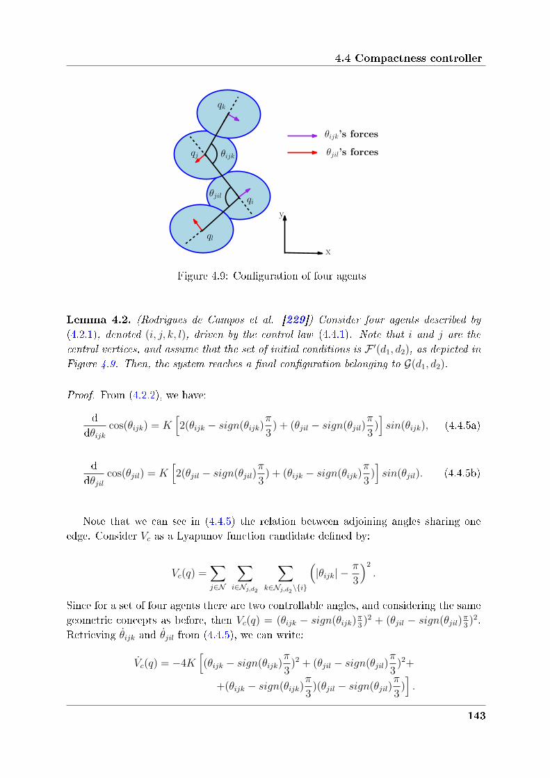
4.4 Compactness controller
qk
qi
qj θijk
y
x
ql
θjil
θijk’s forces
θjil’s forces
Figure 4.9: Conguration of four agents
Lemma 4.2. (Rodrigues de Campos et al. [229]) Consider four agents described by
(4.2.1), denoted (𝑖, 𝑗, 𝑘, 𝑙), driven by the control law (4.4.1). Note that 𝑖 and 𝑗 are the
central vertices, and assume that the set of initial conditions is ℱ ′(𝑑1, 𝑑2), as depicted in
Figure 4.9. Then, the system reaches a final configuration belonging to 𝒢(𝑑1, 𝑑2).
Proof. From (4.2.2), we have:
dd𝜃𝑖𝑗𝑘
cos(𝜃𝑖𝑗𝑘) = 𝐾[2(𝜃𝑖𝑗𝑘 − 𝑠𝑖𝑔𝑛(𝜃𝑖𝑗𝑘)
𝜋
3) + (𝜃𝑗𝑖𝑙 − 𝑠𝑖𝑔𝑛(𝜃𝑗𝑖𝑙)
𝜋
3)]𝑠𝑖𝑛(𝜃𝑖𝑗𝑘), (4.4.5a)
dd𝜃𝑗𝑖𝑙
cos(𝜃𝑗𝑖𝑙) = 𝐾[2(𝜃𝑗𝑖𝑙 − 𝑠𝑖𝑔𝑛(𝜃𝑗𝑖𝑙)
𝜋
3) + (𝜃𝑖𝑗𝑘 − 𝑠𝑖𝑔𝑛(𝜃𝑖𝑗𝑘)
𝜋
3)]𝑠𝑖𝑛(𝜃𝑗𝑖𝑙). (4.4.5b)
Note that we can see in (4.4.5) the relation between adjoining angles sharing oneedge. Consider 𝑉𝑐 as a Lyapunov function candidate dened by:
𝑉𝑐(𝑞) =∑𝑗∈𝒩
∑𝑖∈𝒩𝑗,𝑑2
∑𝑘∈𝒩𝑗,𝑑2
∖𝑖
(|𝜃𝑖𝑗𝑘| −
𝜋
3
)2
.
Since for a set of four agents there are two controllable angles, and considering the samegeometric concepts as before, then 𝑉𝑐(𝑞) = (𝜃𝑖𝑗𝑘 − 𝑠𝑖𝑔𝑛(𝜃𝑖𝑗𝑘)
𝜋3)2 + (𝜃𝑗𝑖𝑙 − 𝑠𝑖𝑔𝑛(𝜃𝑗𝑖𝑙)
𝜋3)2.
Retrieving 𝜃𝑖𝑗𝑘 and 𝜃𝑗𝑖𝑙 from (4.4.5), we can write:
𝑐(𝑞) = −4𝐾[(𝜃𝑖𝑗𝑘 − 𝑠𝑖𝑔𝑛(𝜃𝑖𝑗𝑘)
𝜋
3)2 + (𝜃𝑗𝑖𝑙 − 𝑠𝑖𝑔𝑛(𝜃𝑗𝑖𝑙)
𝜋
3)2+
+(𝜃𝑖𝑗𝑘 − 𝑠𝑖𝑔𝑛(𝜃𝑖𝑗𝑘)𝜋
3)(𝜃𝑗𝑖𝑙 − 𝑠𝑖𝑔𝑛(𝜃𝑗𝑖𝑙)
𝜋
3)].
143
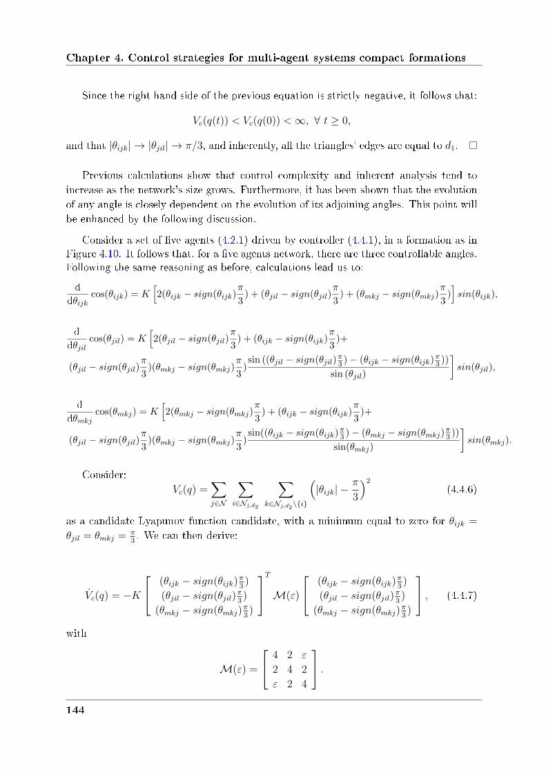
Chapter 4. Control strategies for multi-agent systems compact formations
Since the right hand side of the previous equation is strictly negative, it follows that:
𝑉𝑐(𝑞(𝑡)) < 𝑉𝑐(𝑞(0)) <∞, ∀ 𝑡 ≥ 0,
and that |𝜃𝑖𝑗𝑘| → |𝜃𝑗𝑖𝑙| → 𝜋/3, and inherently, all the triangles' edges are equal to 𝑑1.
Previous calculations show that control complexity and inherent analysis tend toincrease as the network's size grows. Furthermore, it has been shown that the evolutionof any angle is closely dependent on the evolution of its adjoining angles. This point willbe enhanced by the following discussion.
Consider a set of ve agents (4.2.1) driven by controller (4.4.1), in a formation as inFigure 4.10. It follows that, for a ve agents network, there are three controllable angles.Following the same reasoning as before, calculations lead us to:
d
d𝜃𝑖𝑗𝑘cos(𝜃𝑖𝑗𝑘) = 𝐾
[2(𝜃𝑖𝑗𝑘 − 𝑠𝑖𝑔𝑛(𝜃𝑖𝑗𝑘)
𝜋
3) + (𝜃𝑗𝑖𝑙 − 𝑠𝑖𝑔𝑛(𝜃𝑗𝑖𝑙)
𝜋
3) + (𝜃𝑚𝑘𝑗 − 𝑠𝑖𝑔𝑛(𝜃𝑚𝑘𝑗)
𝜋
3)]𝑠𝑖𝑛(𝜃𝑖𝑗𝑘),
d
d𝜃𝑗𝑖𝑙cos(𝜃𝑗𝑖𝑙) = 𝐾
[2(𝜃𝑗𝑖𝑙 − 𝑠𝑖𝑔𝑛(𝜃𝑗𝑖𝑙)
𝜋
3) + (𝜃𝑖𝑗𝑘 − 𝑠𝑖𝑔𝑛(𝜃𝑖𝑗𝑘)
𝜋
3)+
(𝜃𝑗𝑖𝑙 − 𝑠𝑖𝑔𝑛(𝜃𝑗𝑖𝑙)𝜋
3)(𝜃𝑚𝑘𝑗 − 𝑠𝑖𝑔𝑛(𝜃𝑚𝑘𝑗)
𝜋
3)sin ((𝜃𝑗𝑖𝑙 − 𝑠𝑖𝑔𝑛(𝜃𝑗𝑖𝑙)
𝜋3 )− (𝜃𝑖𝑗𝑘 − 𝑠𝑖𝑔𝑛(𝜃𝑖𝑗𝑘)
𝜋3 ))
sin (𝜃𝑗𝑖𝑙)
]𝑠𝑖𝑛(𝜃𝑗𝑖𝑙),
d
d𝜃𝑚𝑘𝑗cos(𝜃𝑚𝑘𝑗) = 𝐾
[2(𝜃𝑚𝑘𝑗 − 𝑠𝑖𝑔𝑛(𝜃𝑚𝑘𝑗)
𝜋
3) + (𝜃𝑖𝑗𝑘 − 𝑠𝑖𝑔𝑛(𝜃𝑖𝑗𝑘)
𝜋
3)+
(𝜃𝑗𝑖𝑙 − 𝑠𝑖𝑔𝑛(𝜃𝑗𝑖𝑙)𝜋
3)(𝜃𝑚𝑘𝑗 − 𝑠𝑖𝑔𝑛(𝜃𝑚𝑘𝑗)
𝜋
3)sin((𝜃𝑖𝑗𝑘 − 𝑠𝑖𝑔𝑛(𝜃𝑖𝑗𝑘)
𝜋3 )− (𝜃𝑚𝑘𝑗 − 𝑠𝑖𝑔𝑛(𝜃𝑚𝑘𝑗)
𝜋3 ))
sin(𝜃𝑚𝑘𝑗)
]𝑠𝑖𝑛(𝜃𝑚𝑘𝑗).
Consider:𝑉𝑐(𝑞) =
∑𝑗∈𝒩
∑𝑖∈𝒩𝑗,𝑑2
∑𝑘∈𝒩𝑗,𝑑2
∖𝑖
(|𝜃𝑖𝑗𝑘| −
𝜋
3
)2
(4.4.6)
as a candidate Lyapunov function candidate, with a minimum equal to zero for 𝜃𝑖𝑗𝑘 =
𝜃𝑗𝑖𝑙 = 𝜃𝑚𝑘𝑗 = 𝜋3. We can then derive:
𝑐(𝑞) = −𝐾
⎡⎣ (𝜃𝑖𝑗𝑘 − 𝑠𝑖𝑔𝑛(𝜃𝑖𝑗𝑘)𝜋3)
(𝜃𝑗𝑖𝑙 − 𝑠𝑖𝑔𝑛(𝜃𝑗𝑖𝑙)𝜋3)
(𝜃𝑚𝑘𝑗 − 𝑠𝑖𝑔𝑛(𝜃𝑚𝑘𝑗)𝜋3)
⎤⎦𝑇 ℳ(𝜀)
⎡⎣ (𝜃𝑖𝑗𝑘 − 𝑠𝑖𝑔𝑛(𝜃𝑖𝑗𝑘)𝜋3)
(𝜃𝑗𝑖𝑙 − 𝑠𝑖𝑔𝑛(𝜃𝑗𝑖𝑙)𝜋3)
(𝜃𝑚𝑘𝑗 − 𝑠𝑖𝑔𝑛(𝜃𝑚𝑘𝑗)𝜋3)
⎤⎦ , (4.4.7)
with
ℳ(𝜀) =
⎡⎣ 4 2 𝜀
2 4 2
𝜀 2 4
⎤⎦ .144
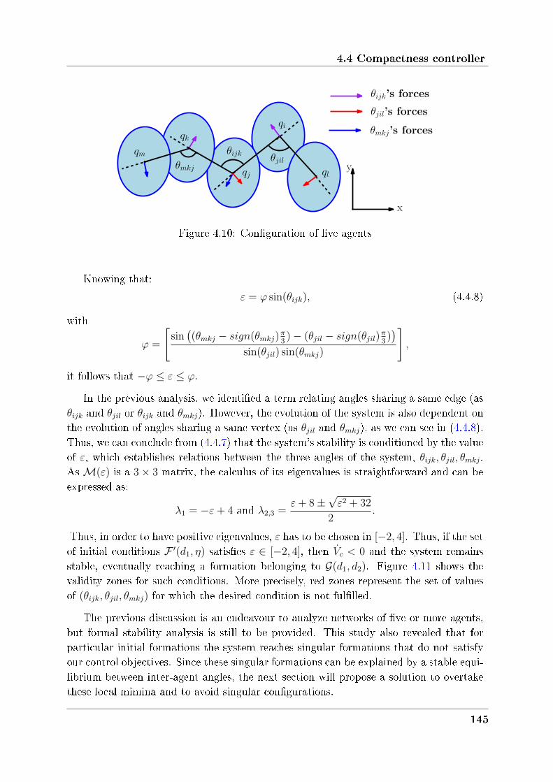
4.4 Compactness controller
qk
qi
qj
θijk
y
x
ql
θjilqm
θmkj
θijk’s forces
θmkj’s forces
θjil’s forces
Figure 4.10: Conguration of ve agents
Knowing that:
𝜀 = 𝜙 sin(𝜃𝑖𝑗𝑘), (4.4.8)
with
𝜙 =
[sin
((𝜃𝑚𝑘𝑗 − 𝑠𝑖𝑔𝑛(𝜃𝑚𝑘𝑗)
𝜋3) − (𝜃𝑗𝑖𝑙 − 𝑠𝑖𝑔𝑛(𝜃𝑗𝑖𝑙)
𝜋3))
sin(𝜃𝑗𝑖𝑙) sin(𝜃𝑚𝑘𝑗)
],
it follows that −𝜙 ≤ 𝜀 ≤ 𝜙.
In the previous analysis, we identied a term relating angles sharing a same edge (as𝜃𝑖𝑗𝑘 and 𝜃𝑗𝑖𝑙 or 𝜃𝑖𝑗𝑘 and 𝜃𝑚𝑘𝑗). However, the evolution of the system is also dependent onthe evolution of angles sharing a same vertex (as 𝜃𝑗𝑖𝑙 and 𝜃𝑚𝑘𝑗), as we can see in (4.4.8).Thus, we can conclude from (4.4.7) that the system's stability is conditioned by the valueof 𝜀, which establishes relations between the three angles of the system, 𝜃𝑖𝑗𝑘, 𝜃𝑗𝑖𝑙, 𝜃𝑚𝑘𝑗.As ℳ(𝜀) is a 3 × 3 matrix, the calculus of its eigenvalues is straightforward and can beexpressed as:
𝜆1 = −𝜀+ 4 and 𝜆2,3 =𝜀+ 8 ±
√𝜀2 + 32
2.
Thus, in order to have positive eigenvalues, 𝜀 has to be chosen in [−2, 4]. Thus, if the setof initial conditions ℱ ′(𝑑1, 𝜂) satises 𝜀 ∈ [−2, 4], then 𝑐 < 0 and the system remainsstable, eventually reaching a formation belonging to 𝒢(𝑑1, 𝑑2). Figure 4.11 shows thevalidity zones for such conditions. More precisely, red zones represent the set of valuesof (𝜃𝑖𝑗𝑘, 𝜃𝑗𝑖𝑙, 𝜃𝑚𝑘𝑗) for which the desired condition is not fullled.
The previous discussion is an endeavour to analyze networks of ve or more agents,but formal stability analysis is still to be provided. This study also revealed that forparticular initial formations the system reaches singular formations that do not satisfyour control objectives. Since these singular formations can be explained by a stable equi-librium between inter-agent angles, the next section will propose a solution to overtakethese local mimina and to avoid singular congurations.
145
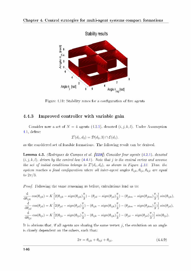
Chapter 4. Control strategies for multi-agent systems compact formations
Figure 4.11: Stability zones for a conguration of ve agents
4.4.3 Improved controller with variable gain
Consider now a set of 𝑁 = 4 agents (4.2.1), denoted (𝑖, 𝑗, 𝑘, 𝑙). Under Assumption4.1, dene:
ℐ ′(𝑑1, 𝑑2) = 𝒟(𝑑2, 3) ∩ ℰ(𝑑1).
as the considered set of feasible formations. The following result can be derived.
Lemma 4.3. (Rodrigues de Campos et al. [229]) Consider four agents (4.2.1), denoted(𝑖, 𝑗, 𝑘, 𝑙), driven by the control law (4.4.1). Note that 𝑗 is the central vertex and assume
the set of initial conditions belongs to ℐ ′(𝑑1, 𝑑2), as shown in Figure 4.12. Thus, the
system reaches a final configuration where all inter-agent angles 𝜃𝑖𝑗𝑘, 𝜃𝑙𝑗𝑖, 𝜃𝑘𝑗𝑙 are equal
to 2𝜋/3.
Proof. Following the same reasoning as before, calculations lead us to:
d
d𝜃𝑖𝑗𝑘cos(𝜃𝑖𝑗𝑘) = 𝐾
[2(𝜃𝑖𝑗𝑘 − 𝑠𝑖𝑔𝑛(𝜃𝑖𝑗𝑘)
𝜋
3)− (𝜃𝑗𝑖𝑙 − 𝑠𝑖𝑔𝑛(𝜃𝑗𝑖𝑙)
𝜋
3)− (𝜃𝑗𝑘𝑚 − 𝑠𝑖𝑔𝑛(𝜃𝑗𝑘𝑚)
𝜋
3)]𝑠𝑖𝑛(𝜃𝑖𝑗𝑘),
d
d𝜃𝑗𝑖𝑙cos(𝜃𝑗𝑖𝑙) = 𝐾
[2(𝜃𝑗𝑖𝑙 − 𝑠𝑖𝑔𝑛(𝜃𝑗𝑖𝑙)
𝜋
3)− (𝜃𝑖𝑗𝑘 − 𝑠𝑖𝑔𝑛(𝜃𝑖𝑗𝑘)
𝜋
3)− (𝜃𝑗𝑘𝑚 − 𝑠𝑖𝑔𝑛(𝜃𝑗𝑘𝑚)
𝜋
3)]𝑠𝑖𝑛(𝜃𝑗𝑖𝑙),
d
d𝜃𝑙𝑗𝑖cos(𝜃𝑙𝑗𝑖) = 𝐾
[2(𝜃𝑙𝑗𝑖 − 𝑠𝑖𝑔𝑛(𝜃𝑙𝑗𝑖)
𝜋
3)− (𝜃𝑖𝑗𝑘 − 𝑠𝑖𝑔𝑛(𝜃𝑖𝑗𝑘)
𝜋
3)− (𝜃𝑗𝑖𝑙 − 𝑠𝑖𝑔𝑛(𝜃𝑗𝑖𝑙)
𝜋
3)]𝑠𝑖𝑛(𝜃𝑙𝑗𝑖).
It is obvious that, if all agents are sharing the same vertex 𝑗, the evolution on an angleis closely dependent on the others, such that:
2𝜋 = 𝜃𝑖𝑗𝑘 + 𝜃𝑘𝑗𝑙 + 𝜃𝑙𝑗𝑖. (4.4.9)
146
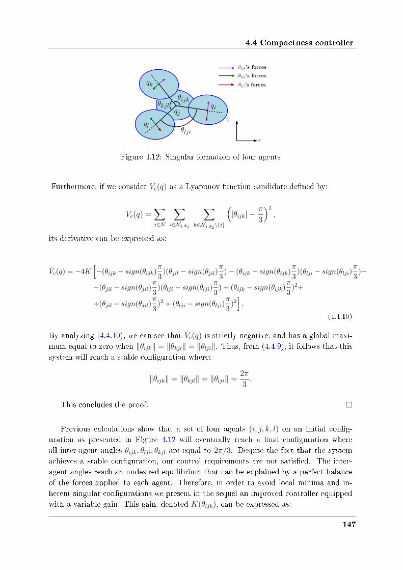
4.4 Compactness controller
qi
ql
qjy
x
qk
θkjl
θlji
θijk
ql
θijk’s forces
θlji’s forces
θkjl’s forces
Figure 4.12: Singular formation of four agents
Furthermore, if we consider 𝑉𝑐(𝑞) as a Lyapunov function candidate dened by:
𝑉𝑐(𝑞) =∑𝑗∈𝒩
∑𝑖∈𝒩𝑗,𝑑2
∑𝑘∈𝒩𝑗,𝑑2
∖𝑖
(|𝜃𝑖𝑗𝑘| −
𝜋
3
)2
,
its derivative can be expressed as:
𝑐(𝑞) = −4𝐾[−(𝜃𝑖𝑗𝑘 − 𝑠𝑖𝑔𝑛(𝜃𝑖𝑗𝑘)
𝜋
3)(𝜃𝑗𝑖𝑙 − 𝑠𝑖𝑔𝑛(𝜃𝑗𝑖𝑙)
𝜋
3)− (𝜃𝑖𝑗𝑘 − 𝑠𝑖𝑔𝑛(𝜃𝑖𝑗𝑘)
𝜋
3)(𝜃𝑙𝑗𝑖 − 𝑠𝑖𝑔𝑛(𝜃𝑙𝑗𝑖)
𝜋
3)−
−(𝜃𝑗𝑖𝑙 − 𝑠𝑖𝑔𝑛(𝜃𝑗𝑖𝑙)𝜋
3)(𝜃𝑙𝑗𝑖 − 𝑠𝑖𝑔𝑛(𝜃𝑙𝑗𝑖)
𝜋
3) + (𝜃𝑖𝑗𝑘 − 𝑠𝑖𝑔𝑛(𝜃𝑖𝑗𝑘)
𝜋
3)2+
+(𝜃𝑗𝑖𝑙 − 𝑠𝑖𝑔𝑛(𝜃𝑗𝑖𝑙)𝜋
3)2 + (𝜃𝑙𝑗𝑖 − 𝑠𝑖𝑔𝑛(𝜃𝑙𝑗𝑖)
𝜋
3)2].
(4.4.10)
By analyzing (4.4.10), we can see that 𝑐(𝑞) is strictly negative, and has a global maxi-mum equal to zero when ‖𝜃𝑖𝑗𝑘‖ = ‖𝜃𝑘𝑗𝑙‖ = ‖𝜃𝑙𝑗𝑖‖. Thus, from (4.4.9), it follows that thissystem will reach a stable conguration where:
‖𝜃𝑖𝑗𝑘‖ = ‖𝜃𝑘𝑗𝑙‖ = ‖𝜃𝑙𝑗𝑖‖ =2𝜋
3.
This concludes the proof.
Previous calculations show that a set of four agents (𝑖, 𝑗, 𝑘, 𝑙) on an initial cong-uration as presented in Figure 4.12 will eventually reach a nal conguration whereall inter-agent angles 𝜃𝑖𝑗𝑘, 𝜃𝑙𝑗𝑖, 𝜃𝑘𝑗𝑙 are equal to 2𝜋/3. Despite the fact that the systemachieves a stable conguration, our control requirements are not satised. The inter-agent angles reach an undesired equilibrium that can be explained by a perfect balanceof the forces applied to each agent. Therefore, in order to avoid local minima and in-herent singular congurations we present in the sequel an improved controller equippedwith a variable gain. This gain, denoted 𝐾(𝜃𝑖𝑗𝑘), can be expressed as:
147
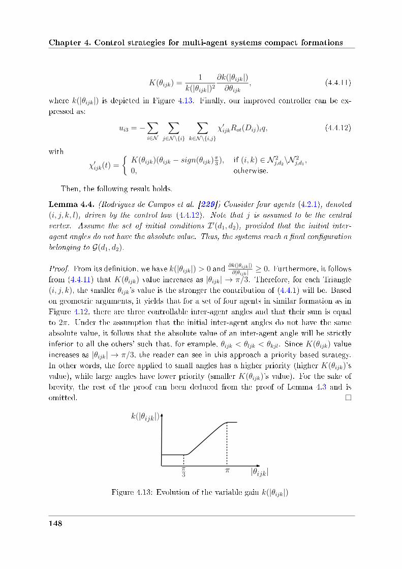
Chapter 4. Control strategies for multi-agent systems compact formations
𝐾(𝜃𝑖𝑗𝑘) =1
𝑘(|𝜃𝑖𝑗𝑘|)2𝜕𝑘(|𝜃𝑖𝑗𝑘|)𝜕𝜃𝑖𝑗𝑘
, (4.4.11)
where 𝑘(|𝜃𝑖𝑗𝑘|) is depicted in Figure 4.13. Finally, our improved controller can be ex-pressed as:
𝑢𝑖3 = −∑𝑖∈𝒩
∑𝑗∈𝒩∖𝑖
∑𝑘∈𝒩∖𝑖,𝑗
𝜒′𝑖𝑗𝑘𝑅𝑜𝑡(𝐷𝑖𝑗)𝑖𝑞, (4.4.12)
with
𝜒′𝑖𝑗𝑘(𝑡) =
𝐾(𝜃𝑖𝑗𝑘)(𝜃𝑖𝑗𝑘 − 𝑠𝑖𝑔𝑛(𝜃𝑖𝑗𝑘)
𝜋3), if (𝑖, 𝑘) ∈ 𝒩 2
𝑗,𝑑2∖𝒩 2
𝑗,𝑑1,
0, otherwise.
Then, the following result holds.
Lemma 4.4. (Rodrigues de Campos et al. [229]) Consider four agents (4.2.1), denoted(𝑖, 𝑗, 𝑘, 𝑙), driven by the control law (4.4.12). Note that 𝑗 is assumed to be the central
vertex. Assume the set of initial conditions ℐ ′(𝑑1, 𝑑2), provided that the initial inter-
agent angles do not have the absolute value. Thus, the systems reach a final configuration
belonging to 𝒢(𝑑1, 𝑑2).
Proof. From its denition, we have 𝑘(|𝜃𝑖𝑗𝑘|) > 0 and 𝜕𝑘(|𝜃𝑖𝑗𝑘|)𝜕|𝜃𝑖𝑗𝑘|
≥ 0. Furthermore, it followsfrom (4.4.11) that 𝐾(𝜃𝑖𝑗𝑘) value increases as |𝜃𝑖𝑗𝑘| → 𝜋/3. Therefore, for each Triangle(𝑖, 𝑗, 𝑘), the smaller 𝜃𝑖𝑗𝑘's value is the stronger the contribution of (4.4.1) will be. Basedon geometric arguments, it yields that for a set of four agents in similar formation as inFigure 4.12, there are three controllable inter-agent angles and that their sum is equalto 2𝜋. Under the assumption that the initial inter-agent angles do not have the sameabsolute value, it follows that the absolute value of an inter-agent angle will be strictlyinferior to all the others' such that, for example, 𝜃𝑖𝑗𝑘 < 𝜃𝑙𝑗𝑘 < 𝜃𝑘𝑗𝑙. Since 𝐾(𝜃𝑖𝑗𝑘) valueincreases as |𝜃𝑖𝑗𝑘| → 𝜋/3, the reader can see in this approach a priority based strategy.In other words, the force applied to small angles has a higher priority (higher 𝐾(𝜃𝑖𝑗𝑘)'svalue), while large angles have lower priority (smaller 𝐾(𝜃𝑖𝑗𝑘)'s value). For the sake ofbrevity, the rest of the proof can been deduced from the proof of Lemma 4.3 and isomitted.
k(|θijk|)
|θijk|π3
π
Figure 4.13: Evolution of the variable gain 𝑘(|𝜃𝑖𝑗𝑘|)
148
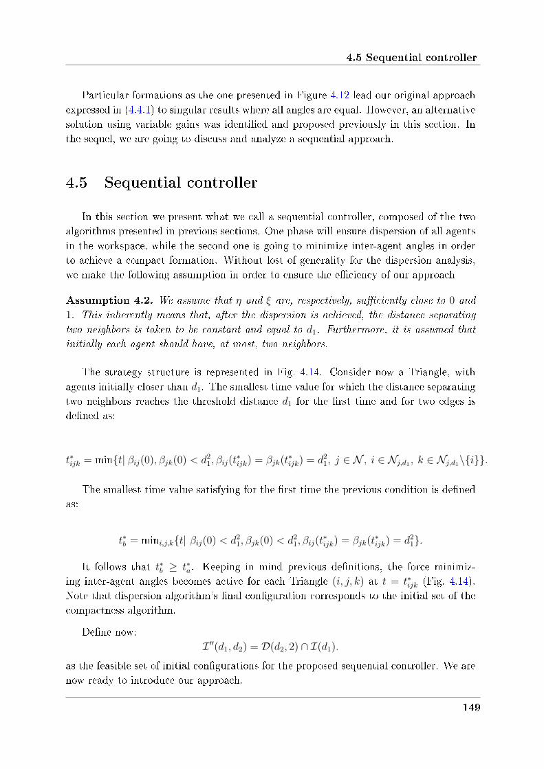
4.5 Sequential controller
Particular formations as the one presented in Figure 4.12 lead our original approachexpressed in (4.4.1) to singular results where all angles are equal. However, an alternativesolution using variable gains was identied and proposed previously in this section. Inthe sequel, we are going to discuss and analyze a sequential approach.
4.5 Sequential controller
In this section we present what we call a sequential controller, composed of the twoalgorithms presented in previous sections. One phase will ensure dispersion of all agentsin the workspace, while the second one is going to minimize inter-agent angles in orderto achieve a compact formation. Without lost of generality for the dispersion analysis,we make the following assumption in order to ensure the eciency of our approach
Assumption 4.2. We assume that 𝜂 and 𝜉 are, respectively, sufficiently close to 0 and
1. This inherently means that, after the dispersion is achieved, the distance separating
two neighbors is taken to be constant and equal to 𝑑1. Furthermore, it is assumed that
initially each agent should have, at most, two neighbors.
The strategy structure is represented in Fig. 4.14. Consider now a Triangle, withagents initially closer than 𝑑1. The smallest time value for which the distance separatingtwo neighbors reaches the threshold distance 𝑑1 for the rst time and for two edges isdened as:
𝑡*𝑖𝑗𝑘 = min𝑡| 𝛽𝑖𝑗(0), 𝛽𝑗𝑘(0) < 𝑑21, 𝛽𝑖𝑗(𝑡*𝑖𝑗𝑘) = 𝛽𝑗𝑘(𝑡
*𝑖𝑗𝑘) = 𝑑21, 𝑗 ∈ 𝒩 , 𝑖 ∈ 𝒩𝑗,𝑑1 , 𝑘 ∈ 𝒩𝑗,𝑑1∖𝑖.
The smallest time value satisfying for the rst time the previous condition is denedas:
𝑡*𝑏 = min𝑖,𝑗,𝑘𝑡| 𝛽𝑖𝑗(0) < 𝑑21, 𝛽𝑗𝑘(0) < 𝑑21, 𝛽𝑖𝑗(𝑡*𝑖𝑗𝑘) = 𝛽𝑗𝑘(𝑡
*𝑖𝑗𝑘) = 𝑑21.
It follows that 𝑡*𝑏 ≥ 𝑡*𝑎. Keeping in mind previous denitions, the force minimiz-ing inter-agent angles becomes active for each Triangle (𝑖, 𝑗, 𝑘) at 𝑡 = 𝑡*𝑖𝑗𝑘 (Fig. 4.14).Note that dispersion algorithm's nal conguration corresponds to the initial set of thecompactness algorithm.
Dene now:ℐ ′′(𝑑1, 𝑑2) = 𝒟(𝑑2, 2) ∩ ℐ(𝑑1).
as the feasible set of initial congurations for the proposed sequential controller. We arenow ready to introduce our approach.
149
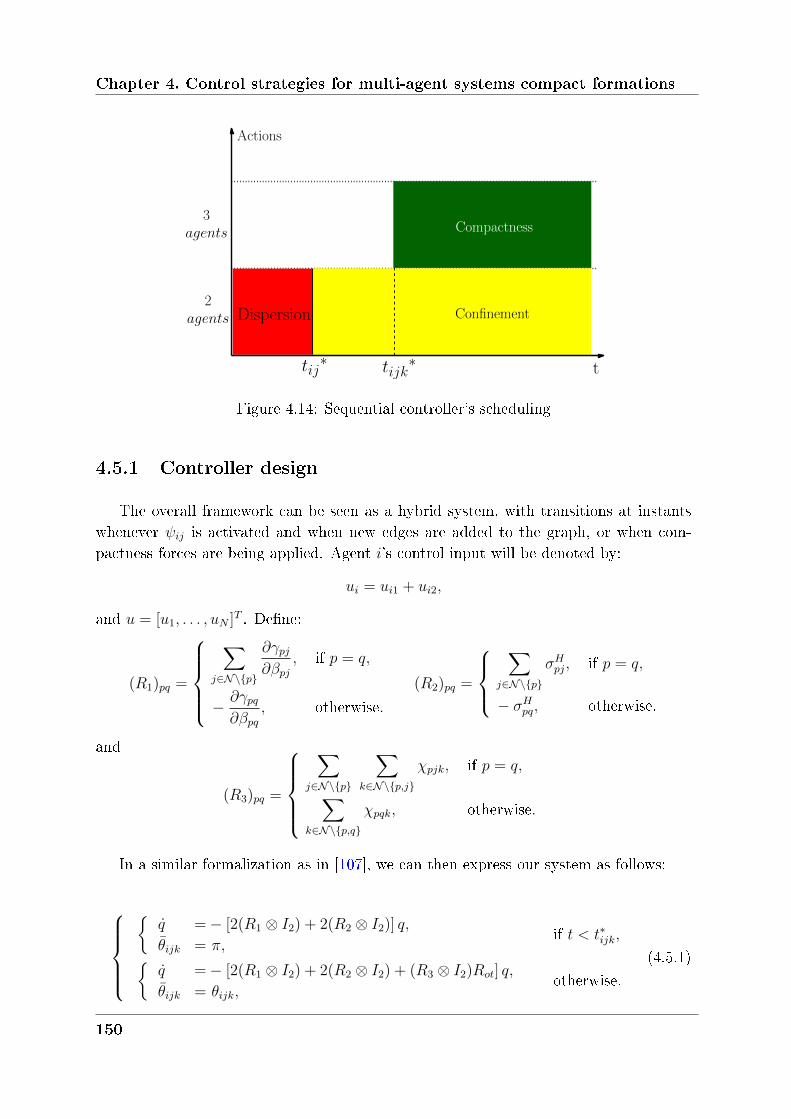
Chapter 4. Control strategies for multi-agent systems compact formations
Dispersion Confinement
tij∗ tijk
∗ t
Actions
2agents
3agents Compactness
Figure 4.14: Sequential controller's scheduling
4.5.1 Controller design
The overall framework can be seen as a hybrid system, with transitions at instantswhenever 𝜓𝑖𝑗 is activated and when new edges are added to the graph, or when com-pactness forces are being applied. Agent 𝑖's control input will be denoted by:
𝑢𝑖 = 𝑢𝑖1 + 𝑢𝑖2,
and 𝑢 = [𝑢1, . . . , 𝑢𝑁 ]𝑇 . Dene:
(𝑅1)𝑝𝑞 =
⎧⎪⎪⎪⎨⎪⎪⎪⎩∑
𝑗∈𝒩∖𝑝
𝜕𝛾𝑝𝑗𝜕𝛽𝑝𝑗
, if 𝑝 = 𝑞,
− 𝜕𝛾𝑝𝑞𝜕𝛽𝑝𝑞
, otherwise.
(𝑅2)𝑝𝑞 =
⎧⎪⎨⎪⎩∑
𝑗∈𝒩∖𝑝
𝜎𝐻𝑝𝑗, if 𝑝 = 𝑞,
− 𝜎𝐻𝑝𝑞, otherwise.
and
(𝑅3)𝑝𝑞 =
⎧⎪⎪⎪⎨⎪⎪⎪⎩∑
𝑗∈𝒩∖𝑝
∑𝑘∈𝒩∖𝑝,𝑗
𝜒𝑝𝑗𝑘, if 𝑝 = 𝑞,∑𝑘∈𝒩∖𝑝,𝑞
𝜒𝑝𝑞𝑘, otherwise.
In a similar formalization as in [107], we can then express our system as follows:
⎧⎪⎪⎪⎨⎪⎪⎪⎩
𝑞 = − [2(𝑅1 ⊗ 𝐼2) + 2(𝑅2 ⊗ 𝐼2)] 𝑞,
𝜃𝑖𝑗𝑘 = 𝜋,if 𝑡 < 𝑡*𝑖𝑗𝑘,
𝑞 = − [2(𝑅1 ⊗ 𝐼2) + 2(𝑅2 ⊗ 𝐼2) + (𝑅3 ⊗ 𝐼2)𝑅𝑜𝑡] 𝑞,
𝜃𝑖𝑗𝑘 = 𝜃𝑖𝑗𝑘,otherwise.
(4.5.1)
150
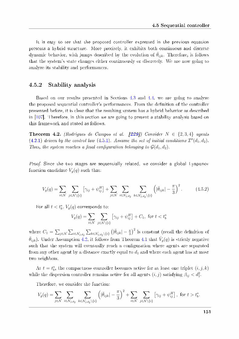
4.5 Sequential controller
It is easy to see that the proposed controller expressed in the previous equationpresents a hybrid structure. More precisely, it exhibits both continuous and discretedynamic behavior, with jumps described by the evolution of 𝜃𝑖𝑗𝑘. Therefore, it followsthat the system's state changes either continuously or discretely. We are now going toanalyze its stability and performances.
4.5.2 Stability analysis
Based on our results presented in Sections 4.3 and 4.4, we are going to analyzethe proposed sequential controller's performances. From the denition of the controllerpresented before, it is clear that the resulting system has a hybrid behavior as describedin [107]. Therefore, in this section we are going to present a stability analysis based onthis framework and stated as follows.
Theorem 4.2. (Rodrigues de Campos et al. [229]) Consider 𝑁 ∈ 2, 3, 4 agents
(4.2.1) driven by the control law (4.5.1). Assume the set of initial conditions ℐ ′′(𝑑1, 𝑑2).
Thus, the system reaches a final configuration belonging to 𝒢(𝑑1, 𝑑2).
Proof. Since the two stages are sequentially related, we consider a global Lyapunovfunction candidate 𝑉𝑔(𝑞) such that:
𝑉𝑔(𝑞) =∑𝑖∈𝒩
∑𝑗∈𝒩∖𝑖
[𝛾𝑖𝑗 + 𝜓𝐻𝑖𝑗
]+∑𝑗∈𝒩
∑𝑖∈𝒩𝑗,𝑑2
∑𝑘∈𝒩𝑗,𝑑2
∖𝑖
(|𝜃𝑖𝑗𝑘| −
𝜋
3
)2
. (4.5.2)
For all 𝑡 < 𝑡*𝑏 , 𝑉𝑔(𝑞) corresponds to:
𝑉𝑔(𝑞) =∑𝑖∈𝒩
∑𝑗∈𝒩∖𝑖
[𝛾𝑖𝑗 + 𝜓𝐻𝑖𝑗
]+ 𝐶1, for 𝑡 < 𝑡*𝑏
where 𝐶1 =∑
𝑗∈𝒩∑
𝑖∈𝒩𝑗,𝑑2
∑𝑘∈𝒩𝑗,𝑑2
∖𝑖(|𝜃𝑖𝑗𝑘| − 𝜋
3
)2is constant (recall the denition of
𝜃𝑖𝑗𝑘). Under Assumption 4.2, it follows from Theorem 4.1 that 𝑔(𝑞) is strictly negativesuch that the system will eventually reach a conguration where agents are separatedfrom any other agent by a distance exactly equal to 𝑑1 and where each agent has at mosttwo neighbors.
At 𝑡 = 𝑡*𝑏 , the compactness controller becomes active for at least one triplet (𝑖, 𝑗, 𝑘)
while the dispersion controller remains active for all agents (𝑖, 𝑗) satisfying 𝛽𝑖𝑗 < 𝑑21.
Therefore, we consider the function:
𝑉𝑔(𝑞) =∑𝑗∈𝒩
∑𝑖∈𝒩𝑗,𝑑2
∑𝑘∈𝒩𝑗,𝑑2
∖𝑖
(|𝜃𝑖𝑗𝑘| −
𝜋
3
)2
+∑𝑖∈𝒩
∑𝑗∈𝒩∖𝑖
[𝛾𝑖𝑗 + 𝜓𝐻𝑖𝑗
], for 𝑡 > 𝑡*𝑏 .
151
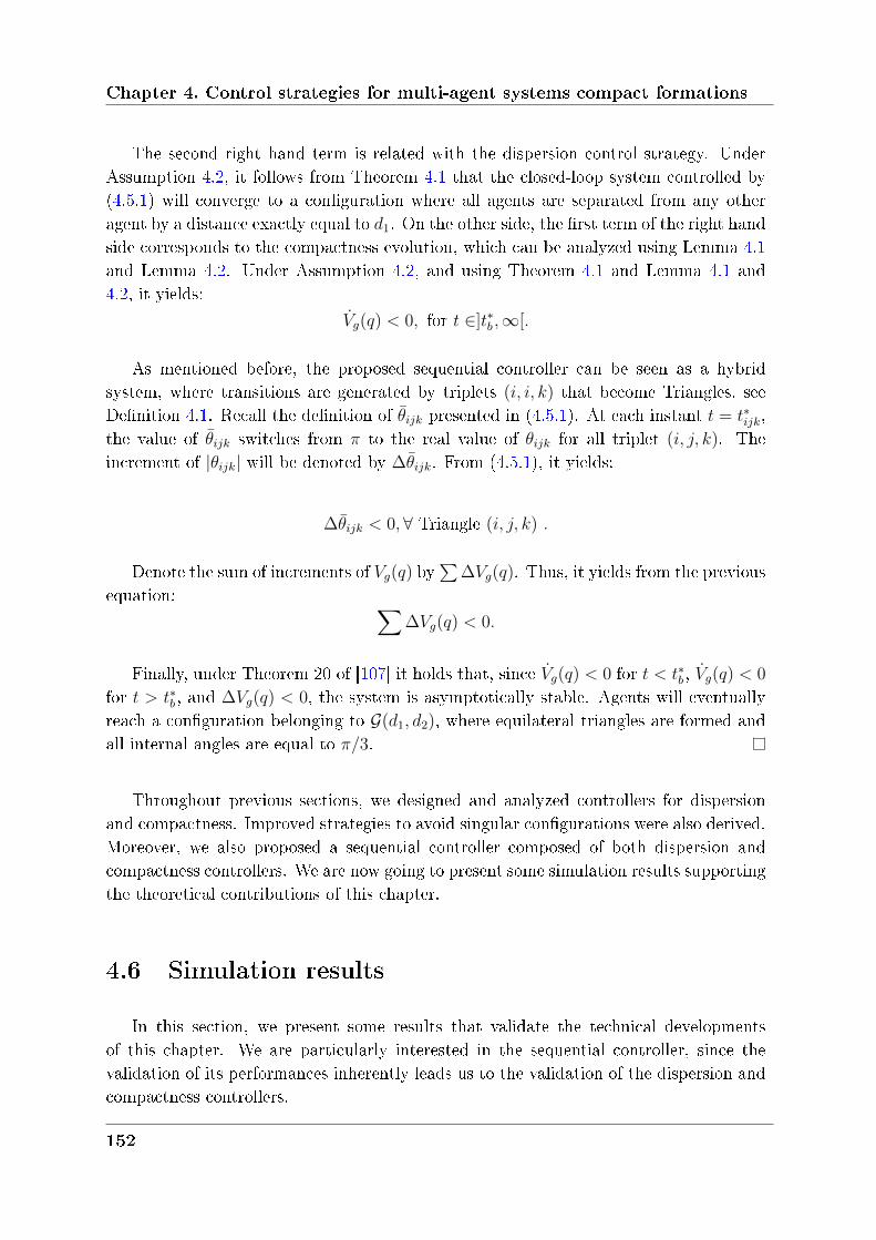
Chapter 4. Control strategies for multi-agent systems compact formations
The second right hand term is related with the dispersion control strategy. UnderAssumption 4.2, it follows from Theorem 4.1 that the closed-loop system controlled by(4.5.1) will converge to a conguration where all agents are separated from any otheragent by a distance exactly equal to 𝑑1. On the other side, the rst term of the right handside corresponds to the compactness evolution, which can be analyzed using Lemma 4.1and Lemma 4.2. Under Assumption 4.2, and using Theorem 4.1 and Lemma 4.1 and4.2, it yields:
𝑔(𝑞) < 0, for 𝑡 ∈]𝑡*𝑏 ,∞[.
As mentioned before, the proposed sequential controller can be seen as a hybridsystem, where transitions are generated by triplets (𝑖, 𝑖, 𝑘) that become Triangles, seeDenition 4.1. Recall the denition of 𝜃𝑖𝑗𝑘 presented in (4.5.1). At each instant 𝑡 = 𝑡*𝑖𝑗𝑘,the value of 𝜃𝑖𝑗𝑘 switches from 𝜋 to the real value of 𝜃𝑖𝑗𝑘 for all triplet (𝑖, 𝑗, 𝑘). Theincrement of |𝜃𝑖𝑗𝑘| will be denoted by ∆𝜃𝑖𝑗𝑘. From (4.5.1), it yields:
∆𝜃𝑖𝑗𝑘 < 0,∀ Triangle (𝑖, 𝑗, 𝑘) .
Denote the sum of increments of 𝑉𝑔(𝑞) by∑
∆𝑉𝑔(𝑞). Thus, it yields from the previousequation: ∑
∆𝑉𝑔(𝑞) < 0.
Finally, under Theorem 20 of [107] it holds that, since 𝑔(𝑞) < 0 for 𝑡 < 𝑡*𝑏 , 𝑔(𝑞) < 0
for 𝑡 > 𝑡*𝑏 , and ∆𝑉𝑔(𝑞) < 0, the system is asymptotically stable. Agents will eventuallyreach a conguration belonging to 𝒢(𝑑1, 𝑑2), where equilateral triangles are formed andall internal angles are equal to 𝜋/3.
Throughout previous sections, we designed and analyzed controllers for dispersionand compactness. Improved strategies to avoid singular congurations were also derived.Moreover, we also proposed a sequential controller composed of both dispersion andcompactness controllers. We are now going to present some simulation results supportingthe theoretical contributions of this chapter.
4.6 Simulation results
In this section, we present some results that validate the technical developmentsof this chapter. We are particularly interested in the sequential controller, since thevalidation of its performances inherently leads us to the validation of the dispersion andcompactness controllers.
152
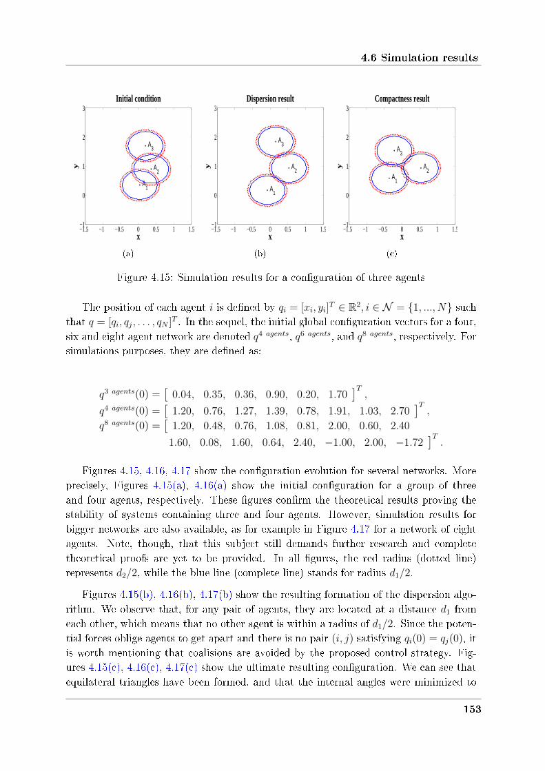
4.6 Simulation results
−1.5 −1 −0.5 0 0.5 1 1.5−1
0
1
2
3
A1
y
x
Initial condition
A2
A3
(a)
−1.5 −1 −0.5 0 0.5 1 1.5−1
0
1
2
3
A1
x
Dispersion result
y A2
A3
(b)
−1.5 −1 −0.5 0 0.5 1 1.5−1
0
1
2
3
A1
x
Compactness result
y A2
A3
(c)
Figure 4.15: Simulation results for a conguration of three agents
The position of each agent 𝑖 is dened by 𝑞𝑖 = [𝑥𝑖, 𝑦𝑖]𝑇 ∈ R2, 𝑖 ∈ 𝒩 = 1, ..., 𝑁 such
that 𝑞 = [𝑞𝑖, 𝑞𝑗, . . . , 𝑞𝑁 ]𝑇 . In the sequel, the initial global conguration vectors for a four,six and eight agent network are denoted 𝑞4 𝑎𝑔𝑒𝑛𝑡𝑠, 𝑞6 𝑎𝑔𝑒𝑛𝑡𝑠, and 𝑞8 𝑎𝑔𝑒𝑛𝑡𝑠, respectively. Forsimulations purposes, they are dened as:
𝑞3 𝑎𝑔𝑒𝑛𝑡𝑠(0) =[
0.04, 0.35, 0.36, 0.90, 0.20, 1.70]𝑇,
𝑞4 𝑎𝑔𝑒𝑛𝑡𝑠(0) =[
1.20, 0.76, 1.27, 1.39, 0.78, 1.91, 1.03, 2.70]𝑇,
𝑞8 𝑎𝑔𝑒𝑛𝑡𝑠(0) =[
1.20, 0.48, 0.76, 1.08, 0.81, 2.00, 0.60, 2.40
1.60, 0.08, 1.60, 0.64, 2.40, −1.00, 2.00, −1.72]𝑇.
Figures 4.15, 4.16, 4.17 show the conguration evolution for several networks. Moreprecisely, Figures 4.15(a), 4.16(a) show the initial conguration for a group of threeand four agents, respectively. These gures conrm the theoretical results proving thestability of systems containing three and four agents. However, simulation results forbigger networks are also available, as for example in Figure 4.17 for a network of eightagents. Note, though, that this subject still demands further research and completetheoretical proofs are yet to be provided. In all gures, the red radius (dotted line)represents 𝑑2/2, while the blue line (complete line) stands for radius 𝑑1/2.
Figures 4.15(b), 4.16(b), 4.17(b) show the resulting formation of the dispersion algo-rithm. We observe that, for any pair of agents, they are located at a distance 𝑑1 fromeach other, which means that no other agent is within a radius of 𝑑1/2. Since the poten-tial forces oblige agents to get apart and there is no pair (𝑖, 𝑗) satisfying 𝑞𝑖(0) = 𝑞𝑗(0), itis worth mentioning that coalisions are avoided by the proposed control strategy. Fig-ures 4.15(c), 4.16(c), 4.17(c) show the ultimate resulting conguration. We can see thatequilateral triangles have been formed, and that the internal angles were minimized to
153
Chapter 4. Control strategies for multi-agent systems compact formations
−0.5 0 0.5 1 1.5 2 2.5−0.5
0
0.5
1
1.5
2
2.5
3
3.5
A1
y
x
Initial condition
A2
A3
A4
(a)
−0.5 0 0.5 1 1.5 2 2.5−0.5
0
0.5
1
1.5
2
2.5
3
3.5
A1
x
Dispersion result
y A2
A3
A4
(b)
−0.5 0 0.5 1 1.5 2 2.5−0.5
0
0.5
1
1.5
2
2.5
3
3.5
A1
x
Compactness result
y
A2
A3
A4
(c)
Figure 4.16: Simulation results for a conguration of four agents
0 1 2 3 4 5−3
−2
−1
0
1
2
3
A1y
x
Initial condition
A2
A3
A4
A5
A6 A
7
A8
(a)
0 1 2 3 4 5−3
−2
−1
0
1
2
3
A1
x
Dispersion result
y
A2
A3
A4
A5
A6 A
7
A8
(b)
0 1 2 3 4 5−3
−2
−1
0
1
2
3
A1
x
Compactness result
y
A2
A3
A4
A5
A6
A7
A8
(c)
Figure 4.17: Simulation results for a conguration of eight agents
𝜋/3 so that formation is the most compact possible. We also observe that agents con-tinue to keep a 𝑑1 distance from any other agent, which shows the compatibility of thedierent components of (4.5.1) and the eciency of the proposed strategy.
Finally, Figure 4.18 show some results for a particular initial conguration depictedin Figure 4.18(a). The initial conditions for such formation are dened as:
𝑞4 𝑎𝑔𝑒𝑛𝑡𝑠(0) =[
0.12 0.36 0.6 1.2 2.1 0.99 1.41 1.8]𝑇.
In Figure 4.18(b) we can observe the resulting conguration when controller (4.4.1)is applied, leading us to a singular equilibrium where all angles are equal to 2𝜋/3. Then,Figure 4.18(c) shows the resulting formation when the controller (4.4.12), using a variable
154
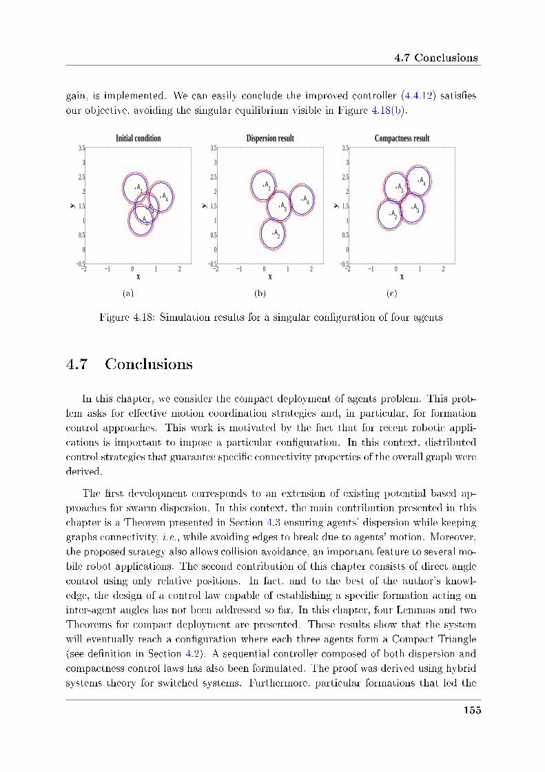
4.7 Conclusions
gain, is implemented. We can easily conclude the improved controller (4.4.12) satisesour objective, avoiding the singular equilibrium visible in Figure 4.18(b).
−2 −1 0 1 2−0.5
0
0.5
1
1.5
2
2.5
3
3.5
A1
y
x
Initial condition
A2
A3
A4
(a)
−2 −1 0 1 2−0.5
0
0.5
1
1.5
2
2.5
3
3.5
A1
x
Dispersion result
y
A2
A3
A4
(b)
−2 −1 0 1 2−0.5
0
0.5
1
1.5
2
2.5
3
3.5
A1
x
Compactness result
y
A2
A3
A4
(c)
Figure 4.18: Simulation results for a singular conguration of four agents
4.7 Conclusions
In this chapter, we consider the compact deployment of agents problem. This prob-lem asks for eective motion coordination strategies and, in particular, for formationcontrol approaches. This work is motivated by the fact that for recent robotic appli-cations is important to impose a particular conguration. In this context, distributedcontrol strategies that guarantee specic connectivity properties of the overall graph werederived.
The rst development corresponds to an extension of existing potential based ap-proaches for swarm dispersion. In this context, the main contribution presented in thischapter is a Theorem presented in Section 4.3 ensuring agents' dispersion while keepinggraphs connectivity, i.e., while avoiding edges to break due to agents' motion. Moreover,the proposed strategy also allows collision avoidance, an important feature to several mo-bile robot applications. The second contribution of this chapter consists of direct anglecontrol using only relative positions. In fact, and to the best of the author's knowl-edge, the design of a control law capable of establishing a specic formation acting oninter-agent angles has not been addressed so far. In this chapter, four Lemmas and twoTheorems for compact deployment are presented. These results show that the systemwill eventually reach a conguration where each three agents form a Compact Triangle(see denition in Section 4.2). A sequential controller composed of both dispersion andcompactness control laws has also been formulated. The proof was derived using hybridsystems theory for switched systems. Furthermore, particular formations that led the
155
Chapter 4. Control strategies for multi-agent systems compact formations
initial system to local minima asked for an improvement of the initial strategy by consid-ering variable gains. To enhance the technical developments of this chapter, simulationresults for several initial congurations and variable number of agents were presented.The simulation setup considers 2-D motion in a cartesian plan. The resulting congura-tions are indeed as compact as possible such that the connectivity of the communicationgraph is optimized. Such feature is extremely important to several cooperative strategiesfor multi-robot systems. In particular, connectivity plays a crucial role on the eciencyand rapidity of distributed protocols. It also allows redundancy, useful for critical appli-cations such as search/recovery and operations in hazardous environnements. Moreover,the resulting geometrically constrained formation may oer a interesting trade-o insome sensor driven applications as, e.g., in gradient search maneuvers.
156
Chapter 5
Conclusions and future works
Contents
5.1 Review of the contributions and conclusions . . . . . . . . . 158
5.1.1 Consensus algorithms . . . . . . . . . . . . . . . . . . . . . . . 158
5.1.2 Compact formations . . . . . . . . . . . . . . . . . . . . . . . . 160
5.2 Ongoing and future works . . . . . . . . . . . . . . . . . . . . 161
5.2.1 Perspectives in consensus algorithms . . . . . . . . . . . . . . . 161
5.2.2 Perspectives in compact formations control . . . . . . . . . . . 162
5.2.3 Perspectives in distributed labeling in artificial populations . . 163
Chapter 5. Conclusions and future works
5.1 Review of the contributions and conclusions
Cooperative control is an important issue due to its large number of applications. Col-laborative behavior of a group of agents means that there exist several interconnectionsbetween them in order to reach a common objective. This thesis pertains to distributedcontrol strategies for multi-robot systems and its applications. Due to the distributedcharacteristics of multi-vehicle systems, the communication graph plays an importantrole in the eciency of control strategies. This manuscript is particulary interested instudying this topic. More precisely, this dissertation presents pertinent results regardingthe motion of a group of vehicles while keeping the best connectivity properties possible.The main contributions of this thesis were developed considering several assumptions onthe agents' model, the communication graph and on the environment. An overview ispresented in the sequel.
5.1.1 Consensus algorithms
Throughout a signicant part of this dissertation a special attention is paid to con-sensus algorithms for heterogeneous agents, representing, for example, dierent modelsor generations of robots. One can easily state that the control complexity of systemsconsidering heterogeneous agents is greater than for simpler frameworks. These workswere motivated by some extremely useful applications demanding for cooperation amongheterogenous agents such as search, recovery or surveillance operations in civil or mil-itary setups. An overview of challenging applications relaying in multi-robots systemsis presented in Chapter 1. It is also worth it mentioning that despite the fact severalworks consider consensus algorithms for homogenous sets of agents, only a few worksconsider heterogeneous cases of the synchronization problem. Furthermore, most of thempresent major drawbacks such as calculation needs, complexity or accuracy of the solu-tion. Chapter 2 proposes an ecient way to simplify the control design for this problem.In this context, the objective is the design of a distributed control law which ensuresthat:
∙ each subsystem is stable;∙ the measurement vectors of each agent reaches an agreement.
More precisely, a control strategy based on consensus algorithms, which is decoupledfrom the original system, was designed in Chapter 2. In other words, we attributedto each agent an additional control variable which achieves a consensus and thus, themeasurement variable of the each agent should converge with this additional variable.
158
5.1 Review of the contributions and conclusions
In these works it is assumed that:
∙ the 𝑁 systems are heterogeneous;∙ each agent 𝑖 ∈ 𝒩 is controllable;∙ for all 𝑖 ∈ 𝒩 , the input vectors directly aects the measurement vector;∙ for all agent 𝑖 ∈ 𝒩 the measurement vectors 𝑧𝑖 represents the same quantity ofinterests for all agents;
∙ the communication graph has a directed spanning tree.
Classical distributed consensus algorithms have been intensively studied in litera-ture. Inherently, their stability and performance properties are well documented. Thewell known convergence properties of simple integrator algorithms naturally motivateit as an appropriated "choice" for the additional dynamics. The rest of the contribu-tion consists of using this trivial consensus algorithm to reach an agreement on thoseadditional dynamics, while applying a model tracking based controller to the remain-ing system. This ensures that the real system will have identical performances as theadditional model. The new algorithm oers the major advantage to separate the sta-bility analysis of each agent and the convergence analysis of the distributed consensusalgorithm. Therefore, it is possible to extend the previous control law to more general sit-uations, where for instance the communication link induces transmission delays or whenone considers distributed lters. Both cases were studied in Chapter 2. However, sev-eral other problems of multi-robot systems can be treated with the proposed approach,and specially simplied. The initial assumptions ask only for a fairly enough connectedgraph and that the input vectors directly aects the measurement vector. Moreover,the presented approach relays in a simpler and lighter structure with respect to [299], arecent result on heterogeneous Multi-Agent Systems (MAS) consensus.
Following the previous study, we were interested in knowing if it is possible to im-prove traditional convergence properties. Consequently, Chapter 3 focuses on consensusalgorithm convergence rate. The speed of convergence of a consensus algorithm, alsocalled algebraic connectivity, is equal to the second smallest eigenvalue of L. Accelerat-ing the convergence of synchronous distributed averaging algorithms have been studiedin literature based on two main approaches: optimizing the topology-respecting weightmatrix summarizing the updates at each node or incorporating memory into the dis-tributed averaging algorithm. Chapter 3 pertains to dealing with this second approach.Even if for most applications delays lead to a reduction of performances or can even leadto instability, there exist some cases where the introduction of a delay in the control loopcan help to stabilize a system. In Chapter 3, a state sampled component is added tothe control law, which can be seen as an articial way to manipulate L's eigenvalues bygetting them further on the left part of the complex plan. The incorporation of memoryin consensus controllers for both simple and double integrator consensus dynamics wasstudied in this manuscript, which proposes and analyzes an eective approach to accel-
159
Chapter 5. Conclusions and future works
erate the convergence of synchronous distributed agreement algorithms. In these worksit is assumed that:
∙ the 𝑁 systems are homogeneous;∙ the communication graph has a directed spanning tree.
In a rst part, the inuence of both partial and global memory in consensus algo-rithms for simple integrator agents was studied. An important conclusion states thatglobal memory drastically improves performances when compared to both trivial andpartial memory based algorithms. An optimization method of the controller parame-ters is proposed so that exponential stability of the solutions is achieved. These resultsare based on discrete-time Lyaponov Theorem and expressed in terms of Linear Ma-trix Inequality (LMI). Also, analytical conditions for improved performances based onLaplacian's eigenvalues were provided. Simulation results show the eciency of the pro-posed algorithm, as well as the conservation of averaging properties. On a second step, anew consensus algorithm for double integrator agents is proposed. For this specic case,Chapter 3 brings forward an improved algorithm that reduces the information quantityneeded for control since velocity sensors' data is not considered. This inherently meanseconomical, space and calculation savings. This work particulary shows the inuenceof articial delays over the system's convergence, since the introduction of a delay inthe control loop helped to stabilize an originally non-stable system. An optimisationmethod of controller parameters is proposed so that exponential stability of the solu-tions is achieved and an expression of the consensus equilibrium is derived with respectto the initial position and velocity of the swarm.
5.1.2 Compact formations
Chapter 4 addresses the design and analysis of an algorithm for compact agent de-ployment. This problem asks for eective motion coordination control strategies and inparticular for formation control approaches. Some of the dierent approaches proposedin recent literature on formation control is provided at the beginning of the chapter.This work is motivated by the fact that for recent robotic applications it is important toimpose a particular conguration. In this context, a special attention was paid to dis-tributed control strategies that guarantee specic connectivity properties of the overallgraph. In the proposed approach, the desired formation is entirely specied by the anglesthat agents within the formation form among themselves. Consequently, a completelydistributed and leaderless algorithm that allows swarm's self-organization is proposed inChapter 4. In these works it is assumed that
∙ the 𝑁 systems are homogeneous;∙ each agent has range based sensing habilites;∙ the initial conguration satises particular conditions.
160
5.2 Ongoing and future works
The rst contribution corresponds to an extension of previous works on swarms disper-sion. By adding a connectivity maintenance force, agents' dispersion is ensured whilekeeping graphs connectivity, i.e., while avoiding edges to break due to agents' motion.Moreover, the proposed strategy also allows collision avoidance, an important feature toseveral mobile robot applications. The second contribution on this topic consists of di-rect angle control since to the best of our knowledge, the design of a control law capableof establishing a specic formation acting on inter-agent angles has not been addressedso far. To solve the compact agent deployment problem inter-agent angles are minimizedin order to achieve the most compact conguration possible, motivated by the fact thatfor successful network operations the deployment should result in congurations thatnot only provide good environment coverage but also satisfy certain local and/or globalconstraints such as the node degree or the network connectivity. Finally, a sequentialproblem composed of both dispersion and compactness control laws is formulated. Theproof has been derived using hybrid systems theory for switched systems. Moreover,since for some particular initial formations the original approach leads to particular andundesired congurations that can be explained by a balance between the inter-agentangles, an improved controller that considers variable gains was also derived.
5.2 Ongoing and future works
This dissertation proposes control strategies to carry out several applications of multi-robot systems. Some interesting areas of future work are outlined in the sequel. Firstly,some nearby extensions of the presented results are described before indicating moredistant research directions.
5.2.1 Perspectives in consensus algorithms
This thesis considers linear MAS that oer good properties for stability analysis. Butin some situations such models are too simple to describe the dynamics of a real agent.Even if an eective solution for linear heterogenous MAS is presented in Chapter 2, anadequate solution to deal with nonlinear heterogenous MAS is still to be provided. Thisis a logical extension of Chapter 2's results.
It is also known that asymptotically stabilizing control design is generally more ac-cessible than nite-time control design, especially for the lack of eective analysis tools.Various nite-time stabilizing control laws have been proposed in literature as for instancein [21, 22, 91, 123, 295, 303, 320]. In particular, nite-time control design has been ex-tended to 𝑛th order systems with both parametric and dynamic uncertainties in [124]and since non-smooth nite-time control synthesis can improve the system behaviors in
161
Chapter 5. Conclusions and future works
some aspects like high-speed, control accuracy, and disturbance- rejection, nite-timecontrol applied to rst order agent dynamics using gradient ow and Lyapunov theorywas proposed in [64]. Even if nite-time distributed control for homogeneous multi-agentsystems was already tackled in literature as for example in [296], there is still free spacefor improvements concerning nite-time consensus algorithms for heterogenous MAS.Considering the decoupled algorithm presented in Chapter 2, those results can likely beextended to t this problem and/or eventually simplify it.
Consider now the results on consensus convergence rate presented in Chapter 3. Asmentioned before, an optimization method of controller parameters and inherent stabilityconditions were expressed in terms of LMI. The proposed solutions consist of o-linecalculations that guarantee exponential stability for a given graph. Even though LMIremains a solid and a powerful tool for the analysis of delayed and sampled systems,they also present some drawbacks. In fact, their complexity will drastically increasefor large networks which can compromise the feasibility of the proposed algorithms.Therefore, in order to overtake these drawbacks for large sized networks, an interestingresearch direction copes with developing other tools for the analysis of memory basedconsensus algorithms. This would considerably reduce the calculation needs and alsothe conservativeness of the initial LMI based conditions. Moreover, this could eventuallylead us to on-line solutions that might be able to calculate the optimal controller settingin real time. On the other hand, an inherent assumption of these works is that allagents are synchronized and share the same clock to ensure that the agents also sharethe same sampling. It is also assumed that the sampling process is periodic. Even if thissetup makes sense in the situation of multi-agents systems, these results might likely beextended to asynchronous samplings. Consequently, it is also logical to consider eventbased control strategies, a useful tool for modern control applications relying on heavycommunication frameworks.
5.2.2 Perspectives in compact formations control
Chapter 4 considers the compact agent deployment problem for linear agents andin particular for simple integrator dynamics. One of the major challenges of this workare the non linearities raised by the angle based control approach. Despite the factthat agents' dynamics correspond to simple integrators, in Section 4.4 the trajectoryof each agent is dependent on the non linear evolution of one or several inter-agentangles. Therefore, the simple initial system becomes through the chosen control strat-egy a highly non linear and constrained system. The presented works revealed that forparticular initial formations the system reaches singular formations that do not satisfythe control objectives. Despite the fact that the system achieves a stable conguration,the control requirements are not fullled: the inter-agent angles reach an singular equi-librium, leading the system to a local minima. But this drawback was overtaken by
162
5.2 Ongoing and future works
considering variable gains. On the other hand, though stability results from dispersionalgorithms for large groups of agents were provided in this manuscript, the compactnesscontroller's analysis is for the moment only valid for three and four agents networks.However, Chapter 4 provides an endeavour to analyze networks of ve or more agents,but formal stability analysis is still to be provided. Therefore, it is pertinent to analysethe eciency of the proposed strategy for high order systems. This analysis should bedone at two levels: one dealing with agent-to-agent relationships, and another, more ab-stract, dealing with edge-to-edge and edge-to-local communication graph relationships.Such an approach would give us insights on how to eciently describe and formalizea multi-agent network based on "edges' neighborhood" instead of the commonly used"agents' neighborhood". Furthermore, one might consider to extend the previous resultto non equal communication radii. This corresponds to a more realistic setup for severalapplications such as, for instance, ship-based radar systems recently studied in [253].
5.2.3 Perspectives in distributed labeling in artificial popula-
tions
Something that has not gained much attention until now is that in an ever chang-ing dynamical environment the agents need to be able to communicate with each otherto improve their adaptability and the overall performance of the group. In the animalkingdom this may be done via the secretion of pheromones or, in the particular exampleof humans, it is done by communicating via Language. This is the main motivation tostudy the possibility of articial agents developing their own Language in the contextof exploring their environment. It is possible to assume that there is no global frame ofreference and there are certain prominent environmental features with unknown globalpositions, beacons or landmarks, such as a communication antenna or an urban land-mark, that all the agents can recognize and can assign a label to. From a control pointof view, it is interesting to investigate the possibility of agents determining each other'spositions via communicating their own position relative to these locally chosen labeledbeacons. To achieve this, it is of course necessary for the agents to agree on the samename for the landmarks, and in a sense develop a Language of their own. A st work inthis work is presented in [233].
Generally speaking, a logical extension of the results presented in this dissertationshould focus on relaxed assumptions in order to consider more realistic situations. Here,we assume perfect communication between two connected vehicles. With a view to an-alyze the performance of the control algorithms previously presented in the presence ofmore realistic communication constraints, cooperative approaches dealing with packetloss, noise and time delays can be considered in further research. Furthermore, through-out this thesis we assume a two-dimensional kinematic model of the vehicles. In conse-
163
Chapter 5. Conclusions and future works
quence, the motions and formations obtained are planar, i.e., the vehicles are movingin a 2-D framework. It would be also pertinent to consider the possibility of developingthree-dimensional motion controllers.
164
Appendix A
Fundamentals on stability of
sampled-data systems
Contents
A.1 Context . . . . . . . . . . . . . . . . . . . . . . . . . . . . . . . 166
A.2 Problem statement . . . . . . . . . . . . . . . . . . . . . . . . 167
A.3 Asymptotic and exponential stability analysis . . . . . . . . 168
A.3.1 Asymptotic stability criteria . . . . . . . . . . . . . . . . . . . . 168
A.3.2 Exponential stability criteria . . . . . . . . . . . . . . . . . . . 169
165
Appendix A. Fundamentals on stability of sampled-data systems
A.1 Context
This appendix looks forward to providing a suciently detailed description of sampledsystems. The sequel completes the results on exponential stability analysis of memorybased consensus algorithms presented in Chapter 3.
The following is based on [250], a relevant work on linear sampled systems. Thisarticle proposes a novel approach to assess stability of continuous linear systems withsampled-data inputs. The method, which is based on the discrete-time Lyapunov theo-rem, provides easy tractable stability conditions for the continuous-time model. Indeed,sucient conditions for asymptotic and exponential stability are provided dealing withsynchronous samplings. This appendix focuses on these results. However, [250] alsocopes with asynchrony, multiple samplings, packet losses and uncertain systems. Butdue to the lack of pertinence within the scope of this thesis, they will be excluded fromthe following discussion.
Networked control systems are generally composed of several distributed plants whichare connected through a communication network. As mentioned before, the existenceof such networks raises several challenges. In the context of this appendix, a heavytemporary load of computation in a processor can corrupt the sampling period of agiven controller. In such situations, the variations of the sampling period will aectthe stability properties. Thus an important issue is the development of robust stabilityconditions with respect to the variations of the sampling period.
Sampled-data systems have been extensively studied in literature, see [47, 98, 100,316, 317] and the references therein. Before presenting important results for systemsunder periodic samplings, let us discuss some works on asynchronous samplings, a morerealistic setup that sill lead to several open problems. Several articles drive the problemof time-varying periods based on a discrete-time approach [122, 187, 271]. An input delayapproach using the Lyapunov-Krasovskii (LK) theorem is provided in [98]. Improvementsare provided in [100, 169], using the small gain theorem and in [182] based on the analysisof impulsive systems. Recently [97, 156, 249] rene those approaches and obtain tighterconditions.
Considering the previously mentioned works, among many others, it is now reasonableto design controllers which guarantee the robustness of the solutions of the closed-loopsystem under periodic samplings. Based on [250], the sequel proposes a novel frameworkfor the stability analysis of linear sampled-data systems using the discrete-time Lya-punov theorem and the continuous-time model of sampled-data systems. In particular,asymptotic and exponential stability criteria are derived from this method to supportthe results presented in Chapter 3. For sake of clearness, the sets N, R+, R𝑛, R𝑛×𝑛 andS𝑛 denote the sets of nonnegative integers, nonnegative scalars, 𝑛-dimensional vectors,𝑛 × 𝑛 matrices and symmetric matrices of R𝑛×𝑛, respectively. Dene K, as the set of
166
A.2 Problem statement
dierentiable functions from an interval of the form [0, 𝑇 ] to R𝑛, where 𝑇 ∈ R+. Thenotation | · | and the superscript `𝑇 ' stand for the Euclidean norm and for matrix trans-position, respectively. The notation 𝑃 > 0 for 𝑃 ∈ S𝑛 means that 𝑃 is positive denite.For any matrix 𝐴 ∈ R𝑛×𝑛, the notation He𝐴 > 0 refers to 𝐴 + 𝐴𝑇 > 0. The symbols𝐼 and 0 represent the identity and the zero matrices of appropriate dimensions.
A.2 Problem statement
Let 𝑡𝑘𝑘∈N be an increasing sequence of positive scalars such that:⋃𝑘∈N
[𝑡𝑘, 𝑡𝑘+1) = [0, +∞),
for which there exist two positive scalars 𝒯1 ≤ 𝒯2 such that:
∀𝑘 ∈ N, 𝑇𝑘 = 𝑡𝑘+1 − 𝑡𝑘 ∈ [𝒯1, 𝒯2]. (A.2.1)
Consider the following sampled-data system:
∀𝑡 ∈ [𝑡𝑘, 𝑡𝑘+1), (𝑡) = 𝐴𝑥(𝑡) +𝐵𝑢(𝑡𝑘), (A.2.2)
where 𝑥 ∈ R𝑛 and 𝑢 ∈ R𝑚 represent the state and the input vectors. The sequence𝑡𝑘𝑘∈N represents the sampling instants of the controller. The matrices 𝐴 and 𝐵 areconstant, known and of appropriate dimension. The control law is a linear state feedback,𝑢 = 𝐾𝑥 with a given gain 𝐾 ∈ R𝑚×𝑛. The system is governed by:
∀𝑡 ∈ [𝑡𝑘, 𝑡𝑘+1), (𝑡) = 𝐴𝑥(𝑡) +𝐵𝐾𝑥(𝑡𝑘). (A.2.3)
Integrating the previous dierential equation, the dynamics of the system satisfy:
∀𝑡 ∈ [𝑡𝑘, 𝑡𝑘+1], 𝑥(𝑡) = Γ(𝑡− 𝑡𝑘)𝑥(𝑡𝑘),
∀𝜏 ∈ [0, 𝑇𝑘], Γ(𝜏) =[𝑒𝐴𝜏 +
∫ 𝜏0𝑒𝐴(𝜏−𝜃)d𝜃𝐵𝐾
].
(A.2.4)
This equality leads naturally to the introduction of the following notation. For anyinteger 𝑘 ∈ N, dene the function 𝜒𝑘 : K, such that, for all 𝜏 ∈ [0, 𝑇𝑘]:
𝜒𝑘(𝜏) = 𝑥(𝑡𝑘 + 𝜏) = Γ(𝜏)𝜒𝑘(0),
𝑘(𝜏) = dd𝜏𝜒𝑘(𝜏) = 𝐴𝜒𝑘(𝜏) +𝐵𝐾𝜒𝑘(0).
(A.2.5)
The denition of 𝜒𝑘 yields 𝑥(𝑡𝑘+1) = 𝜒𝑘(𝑇𝑘) = 𝜒𝑘+1(0).
If 𝐴, 𝐵𝐾 are constant and known and 𝑇𝑘 = 𝒯 , the dynamics become:
𝑥(𝑡𝑘+1) = Γ(𝒯 )𝑥(𝑡𝑘).
167
Appendix A. Fundamentals on stability of sampled-data systems
The system is thus asymptotically stable if and only if Γ(𝒯 ) has all eigenvalues inside theunit circle. If 𝑇𝑘 is time-varying, this does not hold anymore. Relevant stability analysisbased on uncertain representations of Γ(𝑇𝑘) have been already investigated for instancein [121, 187, 271]. Note, though, that extensions to uncertain systems lead to additionaldiculties induced by the denition of Γ. Concerning the analysis using continuous-time models, the input delay approach provided in [98] and rened in [97, 169, 182, 249]leads to relevant stability criteria since it is able to take into account uncertain systems.However, this approach is still conservative in comparison to discrete-time ones. Theresults of [250] establish a novel framework for the stability analysis of sampled-datasystems.
A.3 Asymptotic and exponential stability analysis
In this section, we present asymptotic and exponential stability conditions for syn-chronous sampled-data systems.
A.3.1 Asymptotic stability criteria
The following theorem shows an equivalence between the discrete-time and thecontinuous-time approaches.
Theorem A.1. Let 0 < 𝒯1 ≤ 𝒯2 be two positive scalars and 𝑉 : R𝑛 → R+ be a
differentiable function for which there exist positive scalars 𝜇1 < 𝜇2 and 𝑝 such that:
∀𝑥 ∈ R𝑛, 𝜇1|𝑥|𝑝 ≤ 𝑉 (𝑥) ≤ 𝜇2|𝑥|𝑝. (A.3.1)
Then the two following statements are equivalent.
(i) The increment of the Lyapunov function is strictly negative for all 𝑘 ∈ N and 𝑇𝑘 ∈[𝒯1, 𝒯2], i.e.,
∆0𝑉 (𝑘) = 𝑉 (𝜒𝑘(𝑇𝑘)) − 𝑉 (𝜒𝑘(0)) < 0;
(ii) There exists a continuous and differentiable functional 𝒱0 : [0, 𝒯2] ×K → R which
satisfies for all 𝑧 ∈ K:
∀𝑇 ∈ [𝒯1, 𝒯2] 𝒱0(𝑇, 𝑧(·)) = 𝒱0(0, 𝑧(·)), (A.3.2)
and such that, for all (𝑘, 𝑇𝑘, 𝜏) ∈ N× [𝒯1, 𝒯2] × [0 𝑇𝑘],
0(𝜏, 𝜒𝑘) =d
d𝜏[𝑉 (𝜒𝑘(𝜏)) + 𝒱0(𝜏, 𝜒𝑘)] < 0. (A.3.3)
Moreover, if one of these two statements is satisfied, then the solutions of the system
(A.2.3) are asymptotically stable.
168
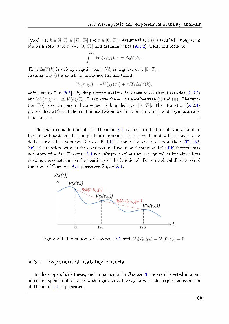
A.3 Asymptotic and exponential stability analysis
Proof. Let 𝑘 ∈ N, 𝑇𝑘 ∈ [𝒯1, 𝑇2] and 𝜏 ∈ [0, 𝑇𝑘]. Assume that (𝑖𝑖) is satised. Integrating0 with respect to 𝜏 over [0, 𝑇𝑘] and assuming that (A.3.2) holds, this leads to:∫ 𝑇𝑘
0
0(𝜏, 𝜒𝑘)d𝜏 = ∆0𝑉 (𝑘).
Then ∆0𝑉 (𝑘) is strictly negative since 0 is negative over [0, 𝑇𝑘].Assume that (𝑖) is satised. Introduce the functional:
𝒱0(𝜏, 𝜒𝑘) = −𝑉 (𝜒𝑘(𝜏)) + 𝜏/𝑇𝑘∆0𝑉 (𝑘),
as in Lemma 2 in [205]. By simple computations, it is easy to see that it satises (A.3.2)and 0(𝜏, 𝜒𝑘) = ∆0𝑉 (𝑘)/𝑇𝑘. This proves the equivalence between (𝑖) and (𝑖𝑖). The func-tion Γ(·) is continuous and consequently bounded over [0, 𝒯2]. Then Equation (A.2.4)proves that 𝑥(𝑡) and the continuous Lyapunov function uniformly and asymptoticallytend to zero.
The main contribution of the Theorem A.1 is the introduction of a new kind ofLyapunov functionals for sampled-data systems. Even though similar functionals werederived from the Lyapunov-Krasovskii (LK) theorem by several other authors [97, 182,249], the relation between the discrete-time Lyapunov theorem and the LK theorem wasnot provided so far. Theorem A.1 not only proves that they are equivalent but also allowsrelaxing the constraint on the positivity of the functional. For a graphical illustration ofthe proof of Theorem A.1, please see Figure A.1.
V(x(t))
tk tk+1 tk+2
V(x(tk))
V(x(tk+1))
V(x(tk+2))
t
WWWW0(t-tk,χk)
WWWW0(t-tk+1,χk+1)
Figure A.1: Illustration of Theorem A.1 with 𝒱0(𝑇𝑘, 𝜒𝑘) = 𝒱0(0, 𝜒𝑘) = 0.
A.3.2 Exponential stability criteria
In the scope of this thesis, and in particular in Chapter 3, we are interested in guar-anteeing exponential stability with a guaranteed decay rate. In the sequel an extensionof Theorem A.1 is presented.
169
Appendix A. Fundamentals on stability of sampled-data systems
Theorem A.2. Consider positive scalars 𝛼, 0 < 𝒯1 ≤ 𝒯2 and a function 𝑉 : R𝑛 → R+,
which satisfies (A.3.1). The two following statements are equivalent.
(i) The function 𝑉 satisfies for all (𝑘, 𝑇𝑘) ∈ N× [𝒯1, 𝒯2]
∆𝛼𝑉 (𝑘) = 𝑒2𝛼𝑇𝑘𝑉 (𝜒𝑘(𝑇𝑘)) − 𝑉 (𝜒𝑘(0)) < 0.
(ii) There exists 𝒱𝛼 : [0, 𝒯2] ×K → R satisfying
∀(𝑇, 𝑧) ∈ [𝒯1, 𝒯2] ×K, 𝑒2𝛼𝑇𝒱𝛼(𝑇, 𝑧(·)) = 𝒱𝛼(0, 𝑧(·)), (A.3.4)
such that the functional 𝒲𝛼(𝜏, 𝜒𝑘) = 𝑒2𝛼𝜏 [𝑉 (𝜒𝑘(𝜏)) +𝒱𝛼(𝜏, 𝜒𝑘)] satisfies
∀(𝑘, 𝑇𝑘, 𝜏) ∈ N× [𝒯1, 𝒯2] × [0, 𝑇𝑘], 𝛼(𝜏, 𝜒𝑘) < 0.
Moreover, if one of these statements holds, the solutions of the system (A.2.3) are expo-nentially stable with the rate 𝛼.
Proof. Consider a given 𝛼 > 0 and a positive integer 𝑘 ∈ N. Following Theorem A.1,(𝑖𝑖) implies (𝑖). Assume now that (𝑖) holds. Consider the functional:
𝒱𝛼(𝜏, 𝜒𝑘) = −𝑉 (𝜒𝑘(𝜏)) + ∆𝛼𝑉 (𝑘)/(𝑒2𝛼𝑇𝑘 − 1).
This functional satises (A.3.4) and
𝛼(𝜏, 𝜒𝑘) =2𝛼𝑇𝑘
𝑒2𝛼𝑇𝑘 − 1
𝑒2𝛼𝜏
𝑇𝑘∆𝛼𝑉 (𝑘).
Since (𝑒2𝛼𝑇𝑘−1)/2𝛼𝑇𝑘 is positive, for all 𝛼, 𝛼 has the same sign as ∆𝛼𝑉 (𝑘). This provesthe equivalence between (𝑖) and (𝑖𝑖). The proof is concluded as in Theorem A.1.
It is worth mentioning that even if 𝛼 < 0, Theorem A.2 still holds. In other words,it means that the solutions of the system can be unstable but the divergence rate of thesolutions is not greater than 𝛼.
This appendix presents some results extracted from [250] that are necessary for acomplete understanding of this thesis, and in particular of Chapter 3. More precisely,these results were used to study the 𝛼−stability of the solutions of memory based con-sensus algorithms under a constant sampling period.
170
Appendix B
Résumé en Français
Sommaire
B.1 Préface . . . . . . . . . . . . . . . . . . . . . . . . . . . . . . . . 173
B.1.1 Introduction . . . . . . . . . . . . . . . . . . . . . . . . . . . . . 173
B.1.2 Contexte de la thèse . . . . . . . . . . . . . . . . . . . . . . . . 176
B.1.3 Structure du document . . . . . . . . . . . . . . . . . . . . . . . 176
B.2 Stratégies de consensus pour des systèmes multi-agents hé-
térogènes . . . . . . . . . . . . . . . . . . . . . . . . . . . . . . 179
B.2.1 Contexte . . . . . . . . . . . . . . . . . . . . . . . . . . . . . . 179
B.2.2 Définition du problème . . . . . . . . . . . . . . . . . . . . . . . 181
B.2.3 Synthèse des lois de commande . . . . . . . . . . . . . . . . . . 182
B.2.4 Loi de commande locale . . . . . . . . . . . . . . . . . . . . . . 183
B.2.5 Loi de commande distribuée . . . . . . . . . . . . . . . . . . . . 183
B.2.6 Extensions à des situations plus complexes . . . . . . . . . . . . 184
B.2.7 Résultats théoriques . . . . . . . . . . . . . . . . . . . . . . . . 185
B.2.8 Résultats de simulation . . . . . . . . . . . . . . . . . . . . . . 185
B.2.9 Conclusions . . . . . . . . . . . . . . . . . . . . . . . . . . . . . 189
B.3 Algorithmes de consensus améliorés par un échantillonnage
approprié . . . . . . . . . . . . . . . . . . . . . . . . . . . . . . 189
B.3.1 Contexte . . . . . . . . . . . . . . . . . . . . . . . . . . . . . . 189
B.3.2 Synthèse des contrôleurs . . . . . . . . . . . . . . . . . . . . . . 192
B.3.3 Définition d’un modèle approprié et résultats théoriques . . . . 192
B.3.4 Résultats de simulation . . . . . . . . . . . . . . . . . . . . . . 194
B.3.5 Conclusions . . . . . . . . . . . . . . . . . . . . . . . . . . . . . 198
B.4 Commande distribuée pour le déploiement compact d’agents 198
B.4.1 Contexte . . . . . . . . . . . . . . . . . . . . . . . . . . . . . . 198
B.4.2 Définition du problème et préliminaires . . . . . . . . . . . . . 200
171
Appendix B. Résumé en Français
B.4.3 Description du système . . . . . . . . . . . . . . . . . . . . . . 200
B.4.4 Définition des fonctions potentielles . . . . . . . . . . . . . . . . 202
B.4.5 Algorithmes de dispersion . . . . . . . . . . . . . . . . . . . . . 203
B.4.6 Synthèse des contrôleurs . . . . . . . . . . . . . . . . . . . . . . 203
B.4.7 Algorithmes de contrôle de la compacité d’une formation . . . . 204
B.4.8 Contrôleur séquentiel . . . . . . . . . . . . . . . . . . . . . . . . 205
B.4.9 Résultats théoriques et de simulation . . . . . . . . . . . . . . . 206
B.4.10 Conclusions . . . . . . . . . . . . . . . . . . . . . . . . . . . . . 207
B.5 Conclusions générales . . . . . . . . . . . . . . . . . . . . . . . 208
B.5.1 Algorithmes de consensus . . . . . . . . . . . . . . . . . . . . . 208
B.5.2 Déploiement compact d’agents . . . . . . . . . . . . . . . . . . 209
172
B.1 Préface
B.1 Préface
B.1.1 Introduction
De nos jours, beaucoup d'infrastructures et de services peuvent facilement être dé-crits par des réseaux d'unités qui interagissent entre eux. On peut trouver des exemplesdans diérents domaines tels que la biologie, les réseaux économiques et, bien sûr, lesdomaines technologiques. Par exemple : Internet, qui est basé sur des milliers de routeurstransmettant des informations partout dans le monde [264] ; les réseaux de distributiond'électricité, composés de centaines de groupes électrogènes qui doivent se synchroniser[203] ; certains systèmes de transport, composés de nombreux éléments [116]. Tous cesexemples exigent des systèmes de contrôles décentralisés où le processus ne réussit qu'aumoment où tous les individus se mettent d'accord sur un certain nombre d'intérêts. Cerésumé en français n'a pas la prétention d'être un document complet sur les travauxde cette thèse. En eet, il n'en présentera que le contexte et les objectifs, ainsi que ladescription des parties les plus pertinentes. Pour l'intégralité des travaux, les preuves ma-thématiques, les résultats élargis ou pour toute information complémentaire, le lecteurest prié de se référer à la version anglaise de la thèse, présentée auparavant.
Bien que les organismes soient, par nature, compétitifs, la coopération entre eux esttrès répandue. Les gènes coopèrent dans le génome, les cellules coopèrent dans les tissus,les individus coopèrent dans les sociétés. Les sociétés animales, dans lesquelles des actionscollectives émergent de la coopération entre individus, ont parfois une grande complexitésociale, voir Figure B.1. Des comportements coopératifs dans de grands groupes d'indi-vidus apparaissent en abondance dans la nature. Il existe des exemples bien connus deces comportements : les bancs de poissons ou les nuées d'oiseaux, voir Figure B.2. Lapropriété fondamentale de cette coopération est que le comportement du groupe n'estpas dicté par l'un des individus [207] : chaque membre suit des règles très simples, chacunagissant suivant des informations locales. Aucun individu ne voit l'image complète. Au-cun individu ne dit à l'autre quoi faire. Curieux et intrigués, quant au mode et à la raisonde la formation de ces groupes et quant à la méthode selon laquelle les rôles joués parchacun y sont déterminés, les scientiques ont tenté de modéliser ces systèmes, symbolesd'une intelligence collective remarquable. La principale question est de savoir commenton peut simuler les diérents comportements de coopération dont témoignent les popu-lations d'oiseaux, d'insectes, etc., sur une population de structures/individus articiels.En utilisant des algorithmes de consensus, un groupe d'agents indépendants doit êtrecapable de résoudre des problèmes d'une manière plus ecace que ce qu'ils pourraientfaire dans le cas où ils seraient contrôlés de manière centralisée. Craig Reynolds a étél'un des premiers à s'intéresser à cette intelligence collective. En 1987, le comportementd'un groupe d'oiseaux en mouvement a été modélisé et simulé dans [227]. Reynolds,qui a réussi à imiter le comportement de groupe, a mené une étude minutieuse sur les
173
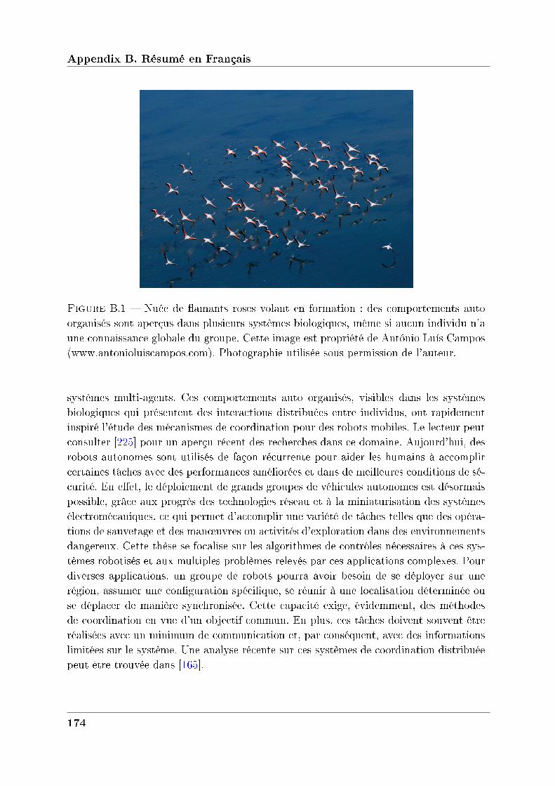
Appendix B. Résumé en Français
Figure B.1 Nuée de amants roses volant en formation : des comportements autoorganisés sont aperçus dans plusieurs systèmes biologiques, même si aucun individu n'aune connaissance globale du groupe. Cette image est propriété de António Luís Campos(www.antonioluiscampos.com). Photographie utilisée sous permission de l'auteur.
systèmes multi-agents. Ces comportements auto organisés, visibles dans les systèmesbiologiques qui présentent des interactions distribuées entre individus, ont rapidementinspiré l'étude des mécanismes de coordination pour des robots mobiles. Le lecteur peutconsulter [225] pour un aperçu récent des recherches dans ce domaine. Aujourd'hui, desrobots autonomes sont utilisés de façon récurrente pour aider les humains à accomplircertaines tâches avec des performances améliorées et dans de meilleures conditions de sé-curité. En eet, le déploiement de grands groupes de véhicules autonomes est désormaispossible, grâce aux progrès des technologies réseau et à la miniaturisation des systèmesélectromécaniques, ce qui permet d'accomplir une variété de tâches telles que des opéra-tions de sauvetage et des man÷uvres ou activités d'exploration dans des environnementsdangereux. Cette thèse se focalise sur les algorithmes de contrôles nécessaires à ces sys-tèmes robotisés et aux multiples problèmes relevés par ces applications complexes. Pourdiverses applications, un groupe de robots pourra avoir besoin de se déployer sur unerégion, assumer une conguration spécique, se réunir à une localisation déterminée ouse déplacer de manière synchronisée. Cette capacité exige, évidemment, des méthodesde coordination en vue d'un objectif commun. En plus, ces tâches doivent souvent êtreréalisées avec un minimum de communication et, par conséquent, avec des informationslimitées sur le système. Une analyse récente sur ces systèmes de coordination distribuéepeut être trouvée dans [165].
174
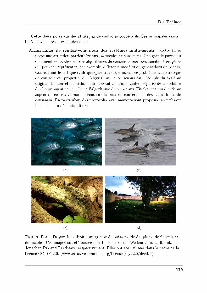
B.1 Préface
Cette thèse porte sur des stratégies de contrôles coopératifs. Ses principales contri-butions sont présentées ci-dessous :
Algorithmes de rendez-vous pour des systèmes multi-agents Cette thèseporte une attention particulière aux protocoles de consensus. Une grande partie dudocument se focalise sur des algorithmes de consensus pour des agents hétérogènesqui peuvent représenter, par exemple, diérents modèles ou générations de robots.Considérant le fait que seuls quelques travaux étudient ce problème, une stratégiede contrôle est proposée, où l'algorithme de consensus est découplé du systèmeoriginal. Le nouvel algorithme ore l'avantage d'une analyse séparée de la stabilitéde chaque agent et de celle de l'algorithme de consensus. Finalement, un deuxièmeaspect de ce travail met l'accent sur le taux de convergence des algorithmes deconsensus. En particulier, des protocoles avec mémoire sont proposés, en utilisantle concept du délai stabilisant.
(a) (b)
(c) (d)
Figure B.2 De gauche à droite, un groupe de poissons, de dauphins, de fourmis etde lucioles. Ces images ont été postées sur Flickr par Tom Weilenmann, Oldbilluk,Jonathan Pio and Lastbeats, respectivement. Elles ont été utilisées dans le cadre de lalicence CC-BY-2.0. (www.creativecommons.org/licenses/by/2.0/deed.fr).
175
Appendix B. Résumé en Français
Algorithmes de déploiement pour des systèmes multi-robots La principalecontribution à ce sujet est un algorithme pour le déploiement compact d'agents.Dans notre approche, la conguration souhaitée est entièrement spéciée par lesangles formés entre agents. Nous avons proposé une solution totalement distribuéequi améliore les propriétés de connectivité du graphe de communication.
B.1.2 Contexte de la thèse
Cette thèse a été élaborée au sein deNetworked Control System Team, une équipeappartenant au Grenoble Images Parole Signal Automatique-Laboratoire et à l'INRIA.Elle fait partie de FeedNetBack 1, nancé par la Commission européenne, et du projetConnect 2, nancé par l'Agence Nationale de la Recherche. Ces deux projets étudientles systèmes commandés en réseau, Networked Control Systems (NCS en anglais), avecune attention particulière portée aux problèmes du contrôle des systèmes multi-agents,c'est-à-dire, des systèmes composés de plusieurs sous-systèmes interconnectés par unréseau de communication hétérogène. Le dé principal de ces projets est d'apprendre àconcevoir des contrôleurs, prenant en compte les contraintes sur la topologie du réseau etsur la possibilité de partager des ressources informatiques, tout en préservant la stabilitédu système. Un cas d'étude commun à ces deux projets se concentre sur la commandecoopérative d'un groupe de véhicules mobiles. Une partie de ces travaux a aussi étédéveloppée dans le cadre du Groupement International de Recherche DelSys, du CentreNational de la Recherche Scientique, qui regroupe plusieurs acteurs scientiques majeursdans ce domaine.
B.1.3 Structure du document
Chapitre 1 : Introduction
Le but de ce chapitre est de détailler les principaux sujets liés à cette thèse et dedonner un aperçu du travail réalisé. Dans un premier temps, nous présentons quelquescomportements coopératifs pour des systèmes multi-agents. La deuxième partie de l'in-troduction porte sur les outils et les approches nécessaires pour ces algorithmes collabora-tifs. Les diérentes applications pour des systèmes multi-agents et les diverses approchesprésentées dans la littérature sont aussi décrites. Finalement, nous y présentons les prin-cipaux dés techniques et les contributions de ce document à ce sujet.
1. www.feednetback.eu/2. www.gipsa-lab.inpg.fr/projet/connect/
176
B.1 Préface
Chapitre 2 : Stratégies de consensus pour des systèmes multi-agents hétéro-
gènes
Le premier objectif de la thèse est le design d'algorithmes de consensus pour desagents hétérogènes qui représentent, par exemple, diérents modèles ou générations derobots. Peu de travaux s'intéressent à ce problème. Les conditions nécessaires et su-santes pour la synchronisation ont été récemment étudiées dans [299]. Dans ce chapitre,nous proposons une stratégie basée sur un algorithme de consensus découplé du systèmed'origine. En d'autres termes, nous attribuons à chaque agent une variable de contrôlesupplémentaire qui atteint un consensus, tout en garantissant une convergence de lavariable d'intérêt de chaque agent vers la variable supplémentaire correspondante. Lenouvel algorithme ore le grand avantage d'une analyse séparée de la stabilité de chaqueagent et de celle de l'algorithme de consensus. Cette conclusion signie fondamentale-ment qu'il est possible d'utiliser d'autres lois de commande plus générales comme, parexemple, des protocoles de consensus avec retards [179, 177, 251] ou des ltres distribués[195]. Ces deux cas sont étudiés dans cette thèse.
Chapitre 3 : Algorithmes de consensus améliorés par un échantillonnage ap-
proprié
Alors que dans le chapitre précédent nous nous sommes concentrés sur la conceptiond'algorithmes de consensus, dans celui-ci nous porterons une attention particulière àleur vitesse de convergence. La vitesse de convergence d'un algorithme de consensuss'avère être égale à la deuxième plus petite valeur propre de L, aussi appelée connectivitéalgébrique. Les moyens pour accélérer la convergence des algorithmes de synchronisationont déjà été étudiés dans la littérature d'après deux approches principales : l'optimisationde la matrice correspondante à la topologie de communication [304] ou l'ajout de mémoiredans l'algorithme. Cette approche sera étudiée dans ce document. Bien que la présencede retards puisse conduire, normalement, à une réduction des performances ou même àl'instabilité, il y a des cas où l'introduction d'un retard dans la boucle de commandepeut aider à stabiliser le système. Cela a été étudié dans [110] et [252]. Pour la deuxièmeapproche, le fait d'ajouter une composante échantillonnée à la loi de commande peut êtreconsidéré comme un moyen articiel pour manipuler les valeurs propres de la matriceLaplacienne et cela signie, implicitement, que la vitesse de convergence changera. Notreobjectif est donc de maximiser cette valeur.
177
Appendix B. Résumé en Français
Chapitre 4 : Stratégies pour le déploiement compact d’un système multi-
robots
Ce troisième chapitre porte sur la conception et l'analyse d'un algorithme de déploie-ment d'un ensemble de robots mobiles. Dans notre approche, la conguration souhaitéeest entièrement spéciée par les angles formés entre les agents. Nous proposons un algo-rithme complètement hiérarchisé et distribué qui permet l'auto organisation du système.La première contribution correspond à une extension de [76] dans des protocoles de dis-persion, où une fonction de maintien de la connectivité a été ajoutée. Chaque agentest équipé d'une fonction potentielle qui, simultanément, permet de l'isoler de tout autreagent et de maintenir la connectivité parmi les agents. La deuxième contribution consisteen un protocole de contrôle des angles inter-agents. Ceci semble être la grande contribu-tion de ce chapitre, étant donné que la synthèse d'une loi de commande, capable d'établirune formation spécique en agissant directement sur les angles inter-agents, n'a pas étéabordée jusqu'à présent. Deux problèmes indépendants ont été traités séparément : ladispersion et la compacité. L'analyse de ces deux stratégies a été faite de façon indé-pendante, mais une structure séquentielle regroupant les deux composantes a aussi étéétudiée. Quelques arguments et calculs, conrmant qu'un tel système correspond à unsystème hybride, sont aussi présentés.
Chapitre 5 : Conclusions et perspectives
Dans ce dernier chapitre de la thèse, nous résumons les contributions de ce travailet nous en décrivons les extensions et les évolutions possibles. De plus, l'Annexe Areprend les principes fondamentaux des systèmes échantillonnés nécessaires à certainsdéveloppements théoriques présentés dans cette thèse.
178
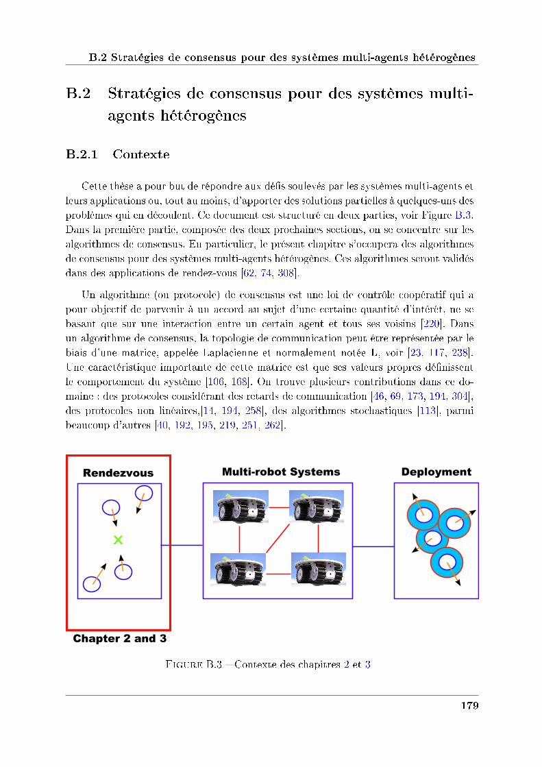
B.2 Stratégies de consensus pour des systèmes multi-agents hétérogènes
B.2 Stratégies de consensus pour des systèmes multi-
agents hétérogènes
B.2.1 Contexte
Cette thèse a pour but de répondre aux dés soulevés par les systèmes multi-agents etleurs applications ou, tout au moins, d'apporter des solutions partielles à quelques-uns desproblèmes qui en découlent. Ce document est structuré en deux parties, voir Figure B.3.Dans la première partie, composée des deux prochaines sections, on se concentre sur lesalgorithmes de consensus. En particulier, le présent chapitre s'occupera des algorithmesde consensus pour des systèmes multi-agents hétérogènes. Ces algorithmes seront validésdans des applications de rendez-vous [62, 74, 308].
Un algorithme (ou protocole) de consensus est une loi de contrôle coopératif qui apour objectif de parvenir à un accord au sujet d'une certaine quantité d'intérêt, ne sebasant que sur une interaction entre un certain agent et tous ses voisins [220]. Dansun algorithme de consensus, la topologie de communication peut être représentée par lebiais d'une matrice, appelée Laplacienne et normalement notée L, voir [23, 117, 238].Une caractéristique importante de cette matrice est que ses valeurs propres dénissentle comportement du système [106, 168]. On trouve plusieurs contributions dans ce do-maine : des protocoles considérant des retards de communication [46, 69, 173, 194, 304],des protocoles non linéaires,[14, 194, 258], des algorithmes stochastiques [113], parmibeaucoup d'autres [40, 192, 195, 219, 251, 262].
Multi-robot Systems
x
Rendezvous Deployment
Chapter 2 and 3
Figure B.3 Contexte des chapitres 2 et 3
179
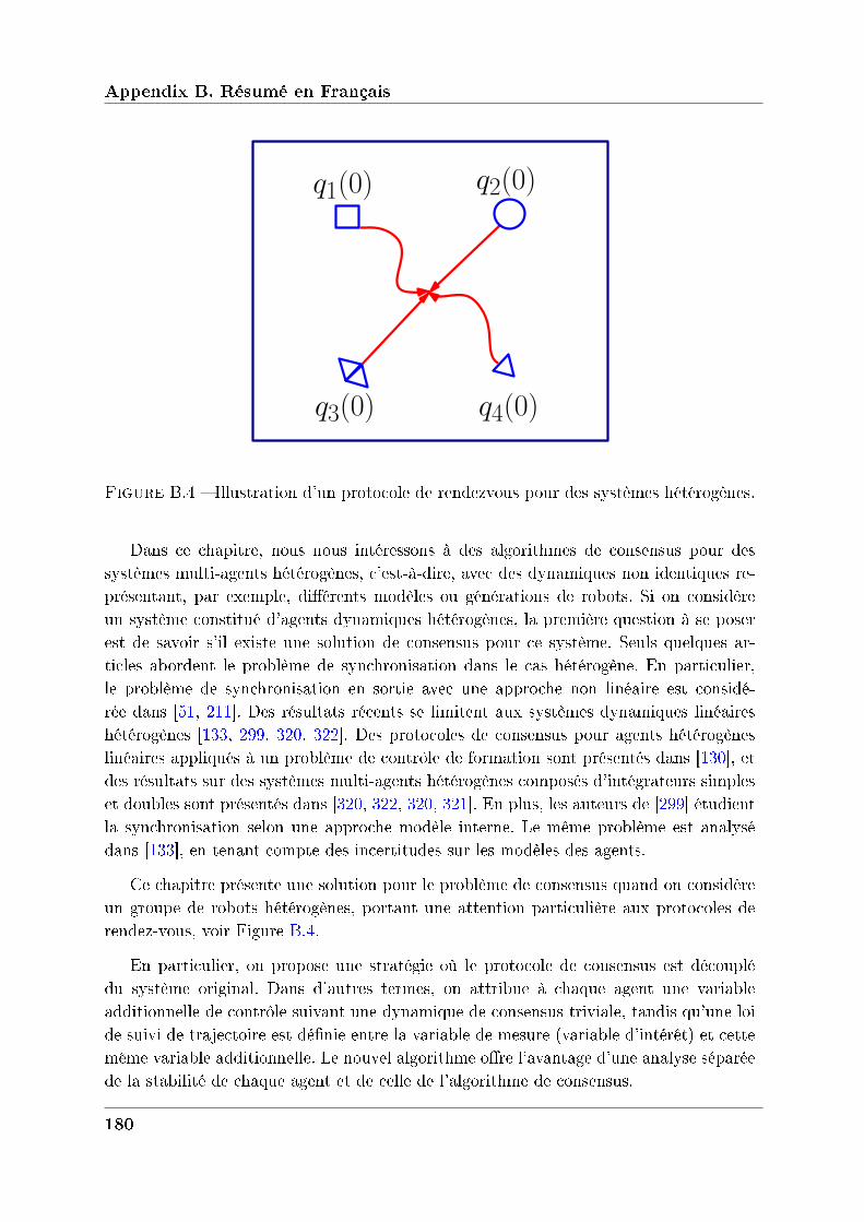
Appendix B. Résumé en Français
q1(0) q2(0)
q3(0) q4(0)
Figure B.4 Illustration d'un protocole de rendezvous pour des systèmes hétérogènes.
Dans ce chapitre, nous nous intéressons à des algorithmes de consensus pour dessystèmes multi-agents hétérogènes, c'est-à-dire, avec des dynamiques non identiques re-présentant, par exemple, diérents modèles ou générations de robots. Si on considèreun système constitué d'agents dynamiques hétérogènes, la première question à se poserest de savoir s'il existe une solution de consensus pour ce système. Seuls quelques ar-ticles abordent le problème de synchronisation dans le cas hétérogène. En particulier,le problème de synchronisation en sortie avec une approche non linéaire est considé-rée dans [51, 211]. Des résultats récents se limitent aux systèmes dynamiques linéaireshétérogènes [133, 299, 320, 322]. Des protocoles de consensus pour agents hétérogèneslinéaires appliqués à un problème de contrôle de formation sont présentés dans [130], etdes résultats sur des systèmes multi-agents hétérogènes composés d'intégrateurs simpleset doubles sont présentés dans [320, 322, 320, 321]. En plus, les auteurs de [299] étudientla synchronisation selon une approche modèle interne. Le même problème est analysédans [133], en tenant compte des incertitudes sur les modèles des agents.
Ce chapitre présente une solution pour le problème de consensus quand on considèreun groupe de robots hétérogènes, portant une attention particulière aux protocoles derendez-vous, voir Figure B.4.
En particulier, on propose une stratégie où le protocole de consensus est découplédu système original. Dans d'autres termes, on attribue à chaque agent une variableadditionnelle de contrôle suivant une dynamique de consensus triviale, tandis qu'une loide suivi de trajectoire est dénie entre la variable de mesure (variable d'intérêt) et cettemême variable additionnelle. Le nouvel algorithme ore l'avantage d'une analyse séparéede la stabilité de chaque agent et de celle de l'algorithme de consensus.
180
B.2 Stratégies de consensus pour des systèmes multi-agents hétérogènes
B.2.2 Définition du problème
Considérons un graphe 𝒢 avec 𝑁 agents et un ensemble d'arêtes déni par 𝐸 =
(𝑖, 𝑗) : 𝑗 ∈ 𝒩𝑖. La matrice d'adjacence peut être dénie par 𝒜 = 𝒜(𝐺) = (𝑎𝑖𝑗), unematrice de dimension 𝑁 ×𝑁 avec 𝑎𝑖𝑗 = 1, si (𝑖, 𝑗) ∈ 𝐸 et 𝑎𝑖𝑗 = 0 sinon.
S'il y a une arête connectant deux n÷uds 𝑖, 𝑗, i.e.,(𝑖, 𝑗) ∈ 𝐸, alors 𝑖, 𝑗 sont désignésvoisins. Le degrée 𝑑𝑖 est déni comme le nombre de voisins d'un n÷ud 𝑖, c'est-à-dire,𝑑𝑖 = #𝑗 : (𝑖, 𝑗) ∈ 𝐸, tel que 𝑑𝑚𝑎𝑥 = 𝑚𝑎𝑥𝑑𝑖. Soit ∆ une matrice diagonale de dimension𝑁×𝑁 , où les élements de la diagonale sont donnés par 𝑑𝑖's. Alors la matrice Laplaciennecorrespondant à 𝒢 est dénie par 𝐿 = ∆ −𝒜.
Dans le vaste domaine des systèmes multi-agents, nous sommes particulièrement in-téressés par les applications de contrôle de robots mobiles dans un plan cartésien. Laposition d'un robot 𝑖 est dénie par :
𝑞𝑖 = [𝑥𝑖, 𝑦𝑖]𝑇 ∈ R2,
où 𝑥𝑖 et 𝑦𝑖 représentent les dynamiques de 𝑞𝑖 dans les axes 𝑥 et 𝑦, respectivement.Cependant, pour des questions de notation et de clarté, nous n'avons pris en comptedans ce chapitre que les dynamiques de chaque agent sur l'axe 𝑥.
Soit le système multi-agents suivant :⎧⎪⎨⎪⎩𝑖 = 𝐴𝑖𝑥𝑖 +𝐵𝑖𝑢𝑖
𝑦𝑖 = 𝑥𝑖
𝑧𝑖 = 𝐶𝑖𝑥𝑖
∀𝑖 ∈ 𝒩 = 1, . . . , 𝑁, (B.2.1)
où 𝑥𝑖 ∈ R𝑛𝑖 , 𝑦𝑖 ∈ R𝑛𝑖 , 𝑧𝑖 ∈ R𝑚 et 𝑢𝑖 ∈ R𝑚 sont les vecteurs des variables d'état, desortie, des variables de mesure et d'entrée, respectivement. On remarque qu'on supposeêtre capable d'accéder à l'état du système, c'est-à-dire, 𝑦𝑖 = 𝑥𝑖 pour tout 𝑖 ∈ 𝒩 . De plus,et pour tout 𝑖 ∈ 𝒩 , on suppose que les matrices 𝐴𝑖 ∈ R𝑛𝑖×𝑛𝑖 , 𝐵𝑖 ∈ R𝑛𝑖×𝑚 et 𝐶𝑖 ∈ R𝑚×𝑛𝑖 ,avec 𝑚 < min𝑛𝑖 et 𝑛𝑖 > 𝑚 sont constantes et connues.
Dans ce contexte, on a pour objectif la synthèse d'une loi de contrôle distribué garan-tissant que (i) chaque système est stable et (ii) que les variables de mesures des systèmesatteignent un consensus. Les hypothèses suivantes sont considérées :
Hypothèse B.1. (Hétérogénéité) : On suppose que les 𝑁 agents sont hétérogènes.
Dans d'autres termes, ceci implique que les dynamiques peuvent varier d'un agent àl'autre et que les vecteurs 𝑥𝑖 peuvent avoir des dimensions diérentes.
Hypothèse B.2. (Homogénéité du vecteur de mesure) : Les vecteurs de mesure 𝑧𝑖sont censé représenter la même quantité d’intérêt pour chaque agent. Donc, les vecteurs
de mesure ont la même dimension, c’est-à-dire, 𝑧𝑖 ∈ R𝑚 ∀𝑖 ∈ 𝒩 , où 𝑚 < min𝑛𝑖.
181
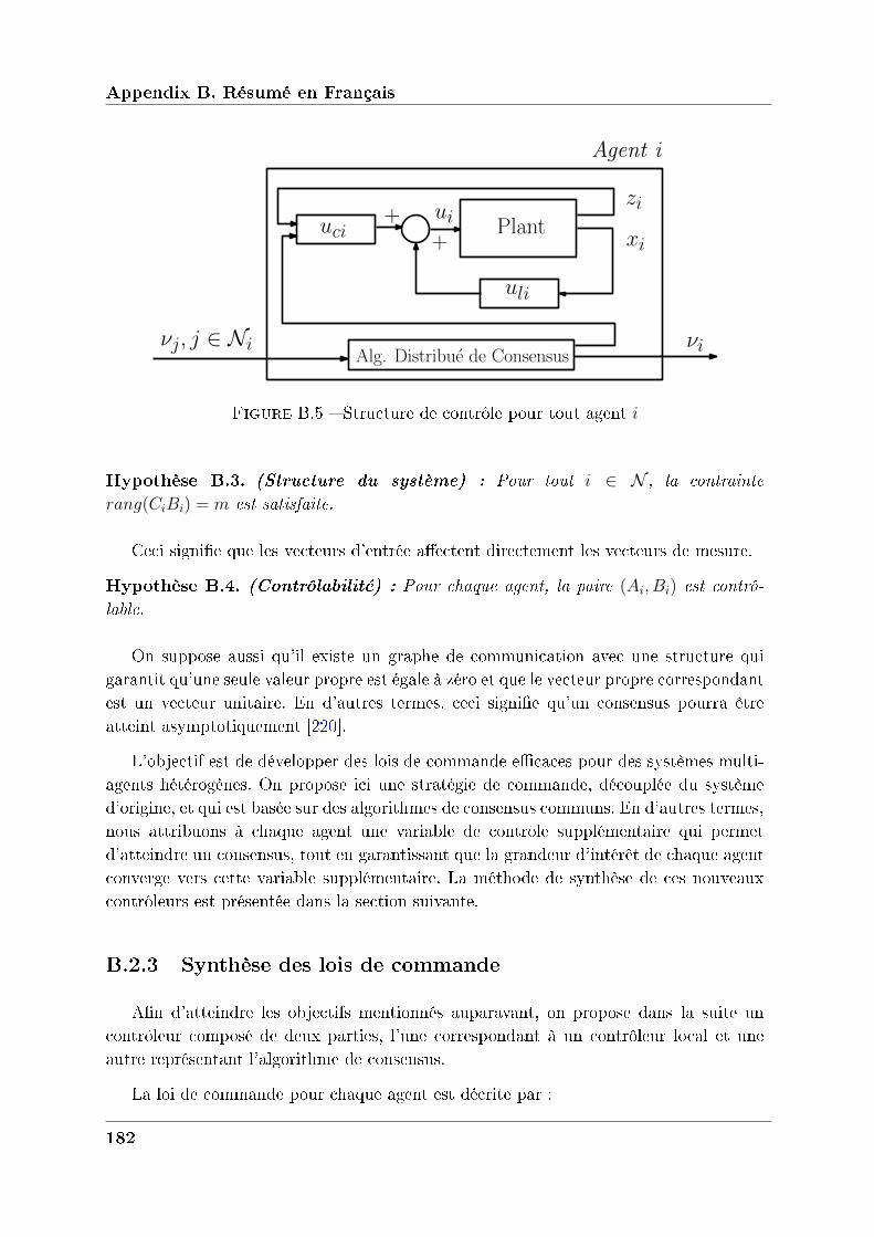
Appendix B. Résumé en Français
Plant
uli
uci
Alg. Distribue de Consensus
++
zi
xi
νiνj, j ∈ Ni
Agent i
ui
Figure B.5 Structure de contrôle pour tout agent 𝑖
Hypothèse B.3. (Structure du système) : Pour tout 𝑖 ∈ 𝒩 , la contrainte
𝑟𝑎𝑛𝑔(𝐶𝑖𝐵𝑖) = 𝑚 est satisfaite.
Ceci signie que les vecteurs d'entrée aectent directement les vecteurs de mesure.
Hypothèse B.4. (Contrôlabilité) : Pour chaque agent, la paire (𝐴𝑖, 𝐵𝑖) est contrô-
lable.
On suppose aussi qu'il existe un graphe de communication avec une structure quigarantit qu'une seule valeur propre est égale à zéro et que le vecteur propre correspondantest un vecteur unitaire. En d'autres termes, ceci signie qu'un consensus pourra êtreatteint asymptotiquement [220].
L'objectif est de développer des lois de commande ecaces pour des systèmes multi-agents hétérogènes. On propose ici une stratégie de commande, découplée du systèmed'origine, et qui est basée sur des algorithmes de consensus communs. En d'autres termes,nous attribuons à chaque agent une variable de contrôle supplémentaire qui permetd'atteindre un consensus, tout en garantissant que la grandeur d'intérêt de chaque agentconverge vers cette variable supplémentaire. La méthode de synthèse de ces nouveauxcontrôleurs est présentée dans la section suivante.
B.2.3 Synthèse des lois de commande
An d'atteindre les objectifs mentionnés auparavant, on propose dans la suite uncontrôleur composé de deux parties, l'une correspondant à un contrôleur local et uneautre représentant l'algorithme de consensus.
La loi de commande pour chaque agent est décrite par :
182
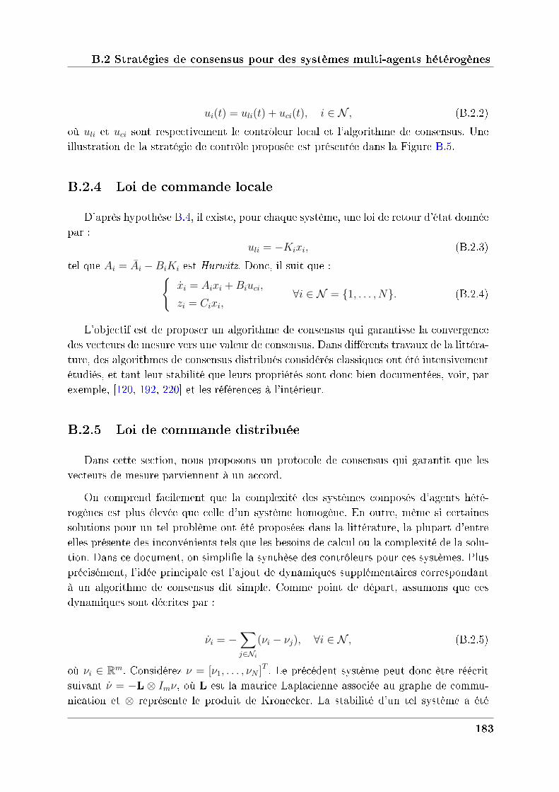
B.2 Stratégies de consensus pour des systèmes multi-agents hétérogènes
𝑢𝑖(𝑡) = 𝑢𝑙𝑖(𝑡) + 𝑢𝑐𝑖(𝑡), 𝑖 ∈ 𝒩 , (B.2.2)
où 𝑢𝑙𝑖 et 𝑢𝑐𝑖 sont respectivement le contrôleur local et l'algorithme de consensus. Uneillustration de la stratégie de contrôle proposée est présentée dans la Figure B.5.
B.2.4 Loi de commande locale
D'après hypothèse B.4, il existe, pour chaque système, une loi de retour d'état donnéepar :
𝑢𝑙𝑖 = −𝐾𝑖𝑥𝑖, (B.2.3)
tel que 𝐴𝑖 = 𝐴𝑖 −𝐵𝑖𝐾𝑖 est Hurwitz. Donc, il suit que :𝑖 = 𝐴𝑖𝑥𝑖 +𝐵𝑖𝑢𝑐𝑖,
𝑧𝑖 = 𝐶𝑖𝑥𝑖,∀𝑖 ∈ 𝒩 = 1, . . . , 𝑁. (B.2.4)
L'objectif est de proposer un algorithme de consensus qui garantisse la convergencedes vecteurs de mesure vers une valeur de consensus. Dans diérents travaux de la littéra-ture, des algorithmes de consensus distribués considérés classiques ont été intensivementétudiés, et tant leur stabilité que leurs propriétés sont donc bien documentées, voir, parexemple, [120, 192, 220] et les références à l'intérieur.
B.2.5 Loi de commande distribuée
Dans cette section, nous proposons un protocole de consensus qui garantit que lesvecteurs de mesure parviennent à un accord.
On comprend facilement que la complexité des systèmes composés d'agents hété-rogènes est plus élevée que celle d'un système homogène. En outre, même si certainessolutions pour un tel problème ont été proposées dans la littérature, la plupart d'entreelles présente des inconvénients tels que les besoins de calcul ou la complexité de la solu-tion. Dans ce document, on simplie la synthèse des contrôleurs pour ces systèmes. Plusprécisément, l'idée principale est l'ajout de dynamiques supplémentaires correspondantà un algorithme de consensus dit simple. Comme point de départ, assumons que cesdynamiques sont décrites par :
𝑖 = −∑𝑗∈𝒩𝑖
(𝜈𝑖 − 𝜈𝑗), ∀𝑖 ∈ 𝒩 , (B.2.5)
où 𝜈𝑖 ∈ R𝑚. Considérez 𝜈 = [𝜈1, . . . , 𝜈𝑁 ]𝑇 . Le précédent système peut donc être réécritsuivant = −L ⊗ 𝐼𝑚𝜈, où L est la matrice Laplacienne associée au graphe de commu-nication et ⊗ représente le produit de Kronecker. La stabilité d'un tel système a été
183
Appendix B. Résumé en Français
largement étudiée dans la littérature comme par exemple dans [192, 220], parmi beau-coup d'autres. Les bonnes propriétés de convergence de l'équation (B.2.5) nous confortedans notre choix d'utiliser ce système comme dynamique supplémentaire. Le reste del'approche consiste à utiliser cet algorithme de consensus bien connu pour parvenir à unaccord sur ces dynamiques supplémentaires, tout en appliquant une loi de suivi entre lesystème original et celui-ci. Cette approche garantit que le système réel aura des perfor-mances identiques à celles du modèle supplémentaire. La synthèse de 𝑢𝑐𝑖 doit considérerles deux objectifs suivants :
⎧⎨⎩ lim𝑡→∞
(𝜈𝑖 − 𝜈𝑗) = 0,
lim𝑡→∞
(𝑧𝑖 − 𝜈𝑖) = 0,∀𝑖, 𝑗 ∈ 𝒩 2. (B.2.6)
Dans cette approche, le système (B.2.5) sera considéré comme le modèle de référencepour (B.2.1). Dénissons le vecteur d'erreur entre le vecteur de mesure 𝑧 du système(B.2.1) et le vecteur de variables additionnelles 𝜈 comme suit :
𝜀𝑖 = 𝑧𝑖 − 𝜈𝑖. (B.2.7)
Le but est donc d'assurer que 𝜀𝑖 convergera vers zéro. Donc, l'évolution de 𝜀𝑖 doit satisfairel'expression suivante :
𝑖 = −𝛽𝜀𝑖,où 𝛽 > 0. Ceci signie que :
𝑖 − 𝑖 = −𝛽(𝑧𝑖 − 𝜈𝑖),
𝐶𝑖(𝐴𝑖𝑥𝑖 +𝐵𝑖𝑢𝑐𝑖) + (L)𝑖 ⊗ 𝐼𝑚𝜈 = −𝛽𝜀, (B.2.8)
où (L)𝑖 représente la 𝑖𝑚𝑒 ligne de la matrice L. D'après hypothèse B.3, 𝐶𝑖𝐵𝑖 est inversiblepour tout agent 𝑖, et donc le contrôleur proposé peut être décrit comme une loi de suivide trajectoire classique, voir [126]. Donc, on peut écrire que :
𝑢𝑐𝑖 = (𝐶𝑖𝐵𝑖)−1 (𝑖 − 𝛽(𝑧𝑖 − 𝜈𝑖) − 𝐶𝑖𝐴𝑖𝑥𝑖) . (B.2.9)
B.2.6 Extensions à des situations plus complexes
C'était notre intuition qu'il était possible de trouver une stratégie peu complexeet avec peu de contraintes sur les moyens de calcul dans le cadre de la synthèse deprotocoles de consensus pour des systèmes hétérogènes. Comme mentionné auparavant,le grand avantage de la méthode proposée réside dans une analyse découplée entre lesdiérents composants du système. Par conséquent, il est possible d'étendre la structureprécédente à des situations plus complexes, en considérant par exemple des retards decommunication [177, 179, 251] ou des ltres distribués [195]. Dans ce document, on aconsidéré, en tant que dynamiques supplémentaires, les deux cas suivants :
184
B.2 Stratégies de consensus pour des systèmes multi-agents hétérogènes
∙ Protocoles de consensus considérant des retards de communication
D'après les résultats de [176, 179], la loi de commande correspondante est donnéepar :
𝑖(𝑡) = 𝐾∑𝑁
𝑗=1𝑎𝑖𝑗𝑑𝑖
(𝜈𝑗(𝑡− 𝜏𝑖𝑗) − 𝜈𝑖(𝑡)) 𝑖 ∈ 1, . . . , 𝑁. (B.2.10)
∙ Protocoles de consensus considérant des références externes
D'après les résultats de [195], la loi de commande correspondante est donnée par :
𝑖 = −𝛼∑𝑗∈𝒩𝑖
(𝜈𝑖 − 𝜈𝑗) +∑𝑗∈𝒥𝑖
(𝑟𝑗 − 𝜈𝑖), (B.2.11)
où 𝒥𝑖 = 𝒩𝑖 ∪ 𝑖 et 𝑟 = [𝑟1, . . . , 𝑟𝑁 ]𝑇 répresente les signaux/références externes.
B.2.7 Résultats théoriques
L'étude des protocoles de consensus distribués appliqués à des systèmes où les agentssont hétérogènes nous a conduits à plusieurs résultats théoriques de cette thèse. Cesrésultats ont été aussi soutenus par des résultats de simulation qui seront présentés plustard dans ce document. Considérant la structure de contrôle présentée dans les sectionsprécédentes, voici notre résultat principal :
Théorème B.1. (Rodrigues de Campos et al. [228]) Si les hypothèses B.1-B.4 sont
satisfaites, alors la loi de commande (B.2.2), donnée par :
𝑢𝑖 = −𝐾𝑖𝑥𝑖 + (𝐶𝑖𝐵𝑖)−1 (𝑖 − 𝛽(𝑧𝑖 − 𝜈𝑖) − 𝐶𝑖𝐴𝑖𝑥𝑖) (B.2.12)
où 𝑖 est défini dans (B.2.5), et garantit que le système multi-agents (B.2.1) est stableet atteint un consensus sur les variables de mesure, c’est-à-dire , 𝑧𝑖 = 𝑧𝑗,∀𝑖, 𝑗 ∈ 𝒩 .
En plus, ce résultat a été étendu à des situations et à des systèmes plus complexes,en considérant diérentes formulations pour les dynamiques supplémentaires présentéesdans (B.2.10) and (B.2.11). L'intégralité de ces résultats est fournie dans le Chapitre 2.
B.2.8 Résultats de simulation
Dans cette section, on ache quelques résultats de simulation concernant l'ecacitéde l'approche présentée précédemment. Dans la suite, on explore un scénario réalisteconsidérant un groupe de robots aériens, voir Figure B.6. On prend un groupe de 𝑁 = 4
agents hétérogènes, dénis par des matrices de diérentes structures et dimensions.
185
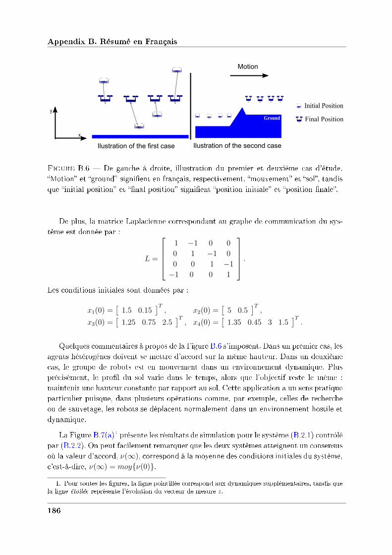
Appendix B. Résumé en Français
y
Ilustration of the first case Ilustration of the second case
Ground
Initial Position
Final Position
x
Motion
Figure B.6 De gauche à droite, illustration du premier et deuxième cas d'étude.Motion et ground signient en français, respectivement, mouvement et sol, tandisque initial position et nal position signient position initiale et position nale.
De plus, la matrice Laplacienne correspondant au graphe de communication du sys-tème est donnée par :
𝐿 =
⎡⎢⎢⎢⎣1 −1 0 0
0 1 −1 0
0 0 1 −1
−1 0 0 1
⎤⎥⎥⎥⎦ .Les conditions initiales sont données par :
𝑥1(0) =[
1.5 0.15]𝑇, 𝑥2(0) =
[5 0.5
]𝑇,
𝑥3(0) =[
1.25 0.75 2.5]𝑇, 𝑥4(0) =
[1.35 0.45 3 1.5
]𝑇.
Quelques commentaires à propos de la Figure B.6 s'imposent. Dans un premier cas, lesagents hétérogènes doivent se mettre d'accord sur la même hauteur. Dans un deuxièmecas, le groupe de robots est en mouvement dans un environnement dynamique. Plusprécisément, le prol du sol varie dans le temps, alors que l'objectif reste le même :maintenir une hauteur constante par rapport au sol. Cette application a un sens pratiqueparticulier puisque, dans plusieurs opérations comme, par exemple, celles de rechercheou de sauvetage, les robots se déplacent normalement dans un environnement hostile etdynamique.
La Figure B.7(a)1 présente les résultats de simulation pour le système (B.2.1) contrôlépar (B.2.2). On peut facilement remarquer que les deux systèmes atteignent un consensusoù la valeur d'accord, 𝜈(∞), correspond à la moyenne des conditions initiales du système,c'est-à-dire, 𝜈(∞) = 𝑚𝑜𝑦𝜈(0).
1. Pour toutes les figures, la ligne pointillée correspond aux dynamiques supplémentaires, tandis quela ligne étoilée représente l’évolution du vecteur de mesure 𝑧.
186
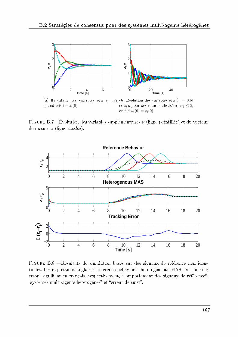
B.2 Stratégies de consensus pour des systèmes multi-agents hétérogènes
0 2 4 60
1
2
3z,
ν
Time [s]
(a) Evolution des variables 𝜈𝑖’s et 𝑧𝑖’s
quand 𝜈𝑖(0) = 𝑧𝑖(0)
0 20 400
1
2
3
z, ν
Time [s]
(b) Evolution des variables 𝜈𝑖’s (𝜏 = 0.6)
et 𝑧𝑖’s pour des retards aléatoires 𝜏𝑖𝑗 ≤ 3,
quand 𝜈𝑖(0) = 𝑧𝑖(0)
Figure B.7 Évolution des variables supplémentaires 𝜈 (ligne pointillée) et du vecteurde mesure 𝑧 (ligne étoilée).
0 2 4 6 8 10 12 14 16 18 20
2
4
r, r
c
Reference Behavior
0 2 4 6 8 10 12 14 16 18 200
5Heterogenous MAS
z, r
c
0 2 4 6 8 10 12 14 16 18 20−2
0
2
Tracking Error
Time [s]
Σ (
z i−r i* )
Figure B.8 Résultats de simulation basés sur des signaux de référence non iden-tiques. Les expressions anglaises reference behavior, heterogeneous MAS et `trackingerror signient en français, respectivement, comportement des signaux de référence,systèmes multi-agents hétérogènes et erreur de suivi.
187
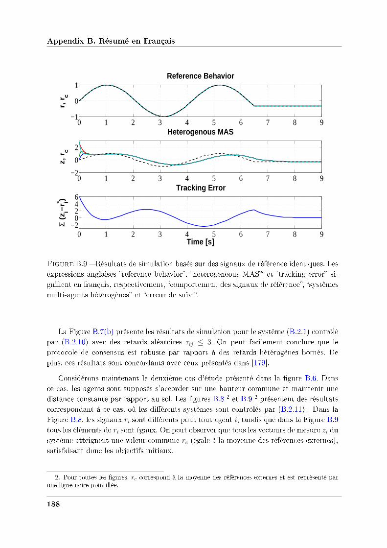
Appendix B. Résumé en Français
0 1 2 3 4 5 6 7 8 9−1
0
1
r, r
c
Reference Behavior
0 1 2 3 4 5 6 7 8 9−2
0
2
Heterogenous MAS
z, r
c
0 1 2 3 4 5 6 7 8 9−2
0246
Tracking Error
Time [s]
Σ (
z i−r i* )
Figure B.9 Résultats de simulation basés sur des signaux de référence identiques. Lesexpressions anglaises reference behavior, heterogeneous MAS` et `tracking error si-gnient en français, respectivement, comportement des signaux de référence, systèmesmulti-agents hétérogènes et erreur de suivi.
La Figure B.7(b) présente les résultats de simulation pour le système (B.2.1) contrôlépar (B.2.10) avec des retards aléatoires 𝜏𝑖𝑗 ≤ 3. On peut facilement conclure que leprotocole de consensus est robuste par rapport à des retards hétérogènes bornés. Deplus, ces résultats sont concordants avec ceux présentés dans [179].
Considérons maintenant le deuxième cas d'étude présenté dans la gure B.6. Dansce cas, les agents sont supposés s'accorder sur une hauteur commune et maintenir unedistance constante par rapport au sol. Les gures B.8 2 et B.9 2 présentent des résultatscorrespondant à ce cas, où les diérents systèmes sont contrôlés par (B.2.11). Dans laFigure B.8, les signaux 𝑟𝑖 sont diérents pout tout agent 𝑖, tandis que dans la Figure B.9tous les éléments de 𝑟𝑖 sont égaux. On peut observer que tous les vecteurs de mesure 𝑧𝑖 dusystème atteignent une valeur commune 𝑟𝑐 (égale à la moyenne des références externes),satisfaisant donc les objectifs initiaux.
2. Pour toutes les figures, 𝑟𝑐 correspond à la moyenne des références externes et est représenté parune ligne noire pointillée.
188
B.3 Algorithmes de consensus améliorés par un échantillonnage approprié
B.2.9 Conclusions
Dans ce chapitre, une nouvelle approche pour la synthèse de lois de commande du typeconsensus a été présentée. D'ailleurs, divers résultats de simulation montrent l'ecacitéde notre approche. Nous avons démontré que, en utilisant des dynamiques supplémen-taires simples, la commande d'un système multi-agents hétérogène devient possible, enmême temps qu'elle limite les contraintes sur le système. Le grand avantage de la mé-thode proposée est de permettre une analyse découplée entre les diérents composantsdu système. Par conséquent, il a été possible d'étendre nos résultats à des situationsplus complexes, en considérant par exemple des retards de communication ou des ltresdistribués avec des références externes.
B.3 Algorithmes de consensus améliorés par un
échantillonnage approprié
B.3.1 Contexte
Cette section porte sur des algorithmes de consensus avec une attention particulièresur leur vitesse de convergence. L'objectif est, plus précisément, l'amélioration des pro-priétés de convergence, en utilisant de la mémoire dans la synthèse des lois de commande.
Pour plusieurs problèmes de contrôle dans le cadre des systèmes multi-agents, lespropriétés de convergence et la vitesse du système dépendent de ce qu'on nomme laconnectivité algébrique du graphe de communication. Plus concrètement, la connectivitéalgébrique est égale à la deuxième plus petite valeur propre de la matrice LaplacienneL. Des méthodes permettant le contrôle de la connectivité du graphe peuvent être trou-vées dans [112, 210, 212, 304, 313, 314], parmi d'autres. En particulier, les travaux de[255] maximisent la connectivité algébrique, sans forcément la calculer, et une approchedistribuée pour l'estimation de la connectivité est présentée dans [4], où les auteurs dé-taillent un scénario du type event-triggered ou, en français, un système déclenché pardes événements.
L'accélération de la vitesse de convergence des algorithmes de consensus a aussi étéétudiée dans la littérature en intégrant de la mémoire dans les lois de commande. C'estprécisément sur cette approche que cette section se focalise. Même si, dans la plupartdes cas, la présence de retards conduit à une réduction des performances ou même àl'instabilité, il y a d'autres scénarios où l'introduction d'un retard dans la boucle decommande peut améliorer les propriétés de convergence du système. Ceci a été étudiédans [110, 252], par exemple.
189
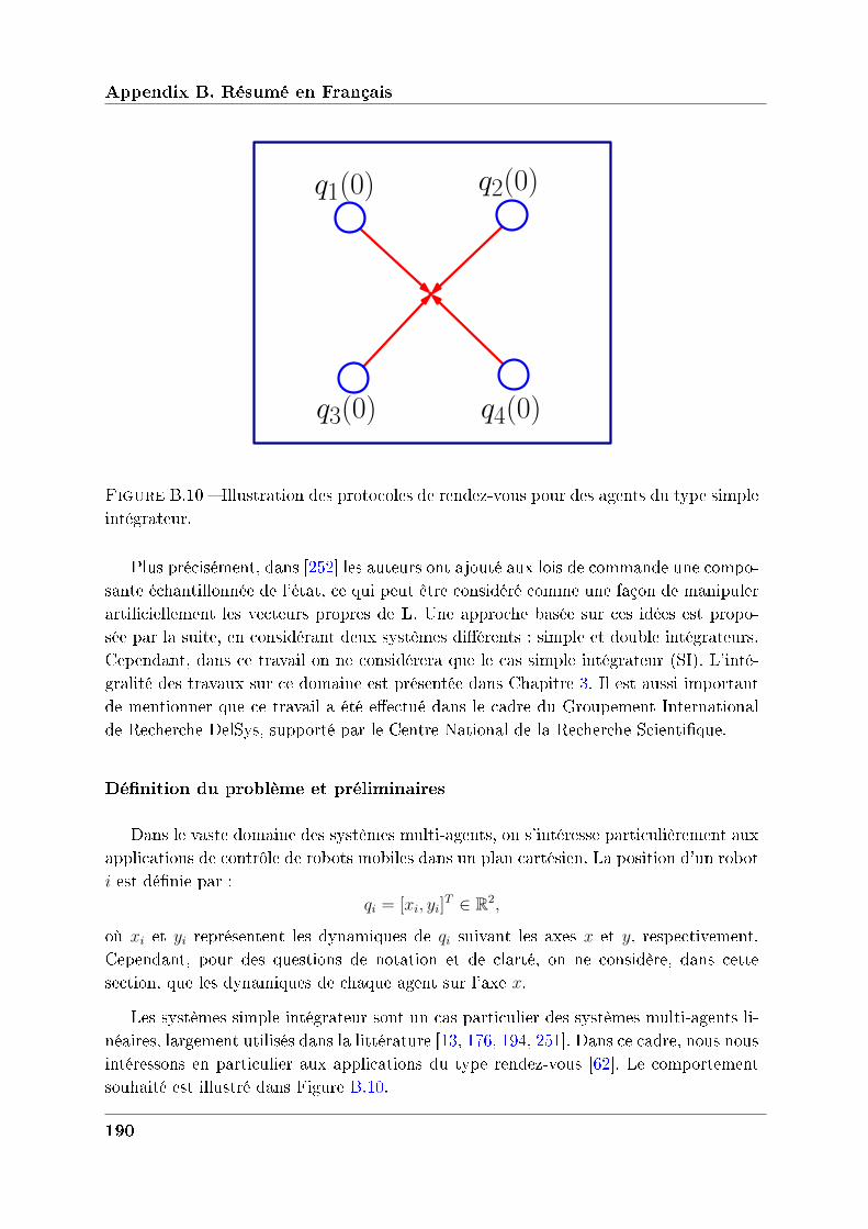
Appendix B. Résumé en Français
q1(0) q2(0)
q3(0) q4(0)
Figure B.10 Illustration des protocoles de rendez-vous pour des agents du type simpleintégrateur.
Plus précisément, dans [252] les auteurs ont ajouté aux lois de commande une compo-sante échantillonnée de l'état, ce qui peut être considéré comme une façon de manipulerarticiellement les vecteurs propres de L. Une approche basée sur ces idées est propo-sée par la suite, en considérant deux systèmes diérents : simple et double intégrateurs.Cependant, dans ce travail on ne considérera que le cas simple intégrateur (SI). L'inté-gralité des travaux sur ce domaine est présentée dans Chapitre 3. Il est aussi importantde mentionner que ce travail a été eectué dans le cadre du Groupement Internationalde Recherche DelSys, supporté par le Centre National de la Recherche Scientique.
Définition du problème et préliminaires
Dans le vaste domaine des systèmes multi-agents, on s'intéresse particulièrement auxapplications de contrôle de robots mobiles dans un plan cartésien. La position d'un robot𝑖 est dénie par :
𝑞𝑖 = [𝑥𝑖, 𝑦𝑖]𝑇 ∈ R2,
où 𝑥𝑖 et 𝑦𝑖 représentent les dynamiques de 𝑞𝑖 suivant les axes 𝑥 et 𝑦, respectivement.Cependant, pour des questions de notation et de clarté, on ne considère, dans cettesection, que les dynamiques de chaque agent sur l'axe 𝑥.
Les systèmes simple intégrateur sont un cas particulier des systèmes multi-agents li-néaires, largement utilisés dans la littérature [13, 176, 194, 251]. Dans ce cadre, nous nousintéressons en particulier aux applications du type rendez-vous [62]. Le comportementsouhaité est illustré dans Figure B.10.
190
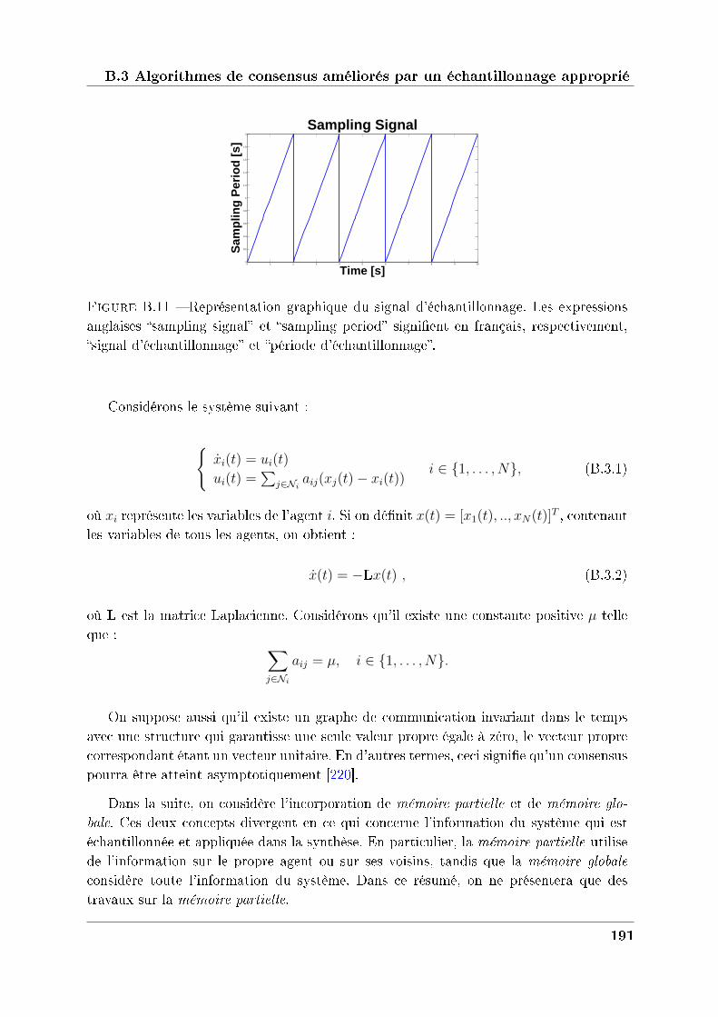
B.3 Algorithmes de consensus améliorés par un échantillonnage approprié
0 1 2 3 4 5 6 7 8 9 100
0.2
0.4
0.6
0.8
1
1.2
1.4
1.6
1.8
2
Time [s]
Sam
plin
g P
erio
d [
s]
Sampling Signal
Figure B.11 Représentation graphique du signal d'échantillonnage. Les expressionsanglaises sampling signal et sampling period signient en français, respectivement,signal d'échantillonnage et période d'échantillonnage.
Considérons le système suivant :
𝑖(𝑡) = 𝑢𝑖(𝑡)
𝑢𝑖(𝑡) =∑
𝑗∈𝒩𝑖𝑎𝑖𝑗(𝑥𝑗(𝑡) − 𝑥𝑖(𝑡))
𝑖 ∈ 1, . . . , 𝑁, (B.3.1)
où 𝑥𝑖 représente les variables de l'agent 𝑖. Si on dénit 𝑥(𝑡) = [𝑥1(𝑡), .., 𝑥𝑁(𝑡)]𝑇 , contenantles variables de tous les agents, on obtient :
(𝑡) = −L𝑥(𝑡) , (B.3.2)
où L est la matrice Laplacienne. Considérons qu'il existe une constante positive 𝜇 telleque : ∑
𝑗∈𝒩𝑖
𝑎𝑖𝑗 = 𝜇, 𝑖 ∈ 1, . . . , 𝑁.
On suppose aussi qu'il existe un graphe de communication invariant dans le tempsavec une structure qui garantisse une seule valeur propre égale à zéro, le vecteur proprecorrespondant étant un vecteur unitaire. En d'autres termes, ceci signie qu'un consensuspourra être atteint asymptotiquement [220].
Dans la suite, on considère l'incorporation de mémoire partielle et de mémoire glo-
bale. Ces deux concepts divergent en ce qui concerne l'information du système qui estéchantillonnée et appliquée dans la synthèse. En particulier, la mémoire partielle utilisede l'information sur le propre agent ou sur ses voisins, tandis que la mémoire globale
considère toute l'information du système. Dans ce résumé, on ne présentera que destravaux sur la mémoire partielle.
191
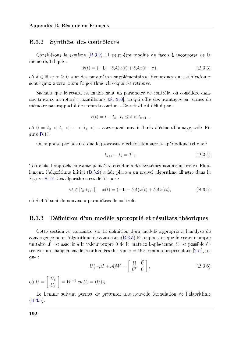
Appendix B. Résumé en Français
B.3.2 Synthèse des contrôleurs
Considérons le système (B.3.2). Il peut être modié de façon à incorporer de lamémoire, tel que :
(𝑡) = (−L− 𝛿𝒜)𝑥(𝑡) + 𝛿𝒜𝑥(𝑡− 𝜏), (B.3.3)
où 𝛿 ∈ R et 𝜏 ≥ 0 sont des paramètres supplémentaires. Remarquez que, si 𝛿 et/ou 𝜏sont égaux à zéro, alors l'algorithme classique est retrouvé.
Sachant que le retard est maintenant un paramètre de contrôle, on considère dansnos travaux un retard échantillonné [98, 250], ce qui ore des avantages en termes demémoire par rapport à des retards continus. Ce retard est déni par :
𝜏(𝑡) = 𝑡− 𝑡𝑘, 𝑡𝑘 ≤ 𝑡 < 𝑡𝑘+1 ,
où 0 = 𝑡0 < 𝑡1 < ... < 𝑡𝑘 < ... correspond aux instants d'échantillonnage, voir Fi-gure B.11.
On suppose par la suite que le processus d'échantillonnage est périodique tel que :
𝑡𝑘+1 − 𝑡𝑘 = 𝑇 . (B.3.4)
Toutefois, l'approche suivante peut être étendue à des systèmes non asynchrones. Fina-lement, l'algorithme initial (B.3.2) a fait place à un nouvel algorithme illustré dans laFigure B.12. Cet algorithme est déni par :
∀𝑡 ∈ [𝑡𝑘 𝑡𝑘+1[, (𝑡) = (−L− 𝛿𝒜)𝑥(𝑡) + 𝛿𝒜𝑥(𝑡𝑘), (B.3.5)
où 𝛿 et 𝑇 sont de nouveaux paramètres de contrôle.
B.3.3 Définition d’un modèle approprié et résultats théoriques
Cette section se concentre sur la dénition d'un modèle approprié à l'analyse deconvergence pour l'algorithme de consensus (B.3.5) En supposant que le vecteur propreunitaire
−→1 est associé à la valeur propre 0 de la matrice Laplacienne, il est possible de
trouver un changement de coordonnées du type 𝑥 = 𝑊𝑧, comme proposé dans [251], telque :
𝑈(−𝜇𝐼 + 𝒜)𝑊 =
[Ω 0
0𝑇 0
], (B.3.6)
où 𝑈 =
[𝑈1
𝑈2
]= 𝑊−1 et 𝑈2 = (𝑈)𝑁 .
Le Lemme suivant permet de présenter une nouvelle formulation de l'algorithme(B.3.5).
192
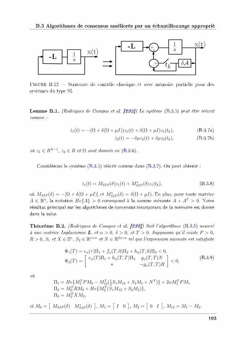
B.3 Algorithmes de consensus améliorés par un échantillonnage approprié
-L x(t)
δA
+x(t)
tk-+
+1s
1s-L
Figure B.12 Structure de contrôle classique et avec mémoire partielle pour dessystèmes du type SI.
Lemme B.1. (Rodrigues de Campos et al. [232]) Le système (B.3.5) peut être réécrit
comme :
1(𝑡) = −(Ω + 𝛿(Ω + 𝜇𝐼))𝑧1(𝑡) + 𝛿(Ω + 𝜇𝐼)𝑧1(𝑡𝑘), (B.3.7a)
2(𝑡) = −𝛿𝜇𝑧2(𝑡) + 𝛿𝜇𝑧2(𝑡𝑘), (B.3.7b)
où 𝑧1 ∈ 𝑅𝑁−1, 𝑧2 ∈ 𝑅 et Ω sont donnés en (B.3.6).
Considérons le système (B.3.5) réécrit comme dans (B.3.7). On peut obtenir :
1(𝑡) = 𝑀𝑆𝐼𝑃 (𝛿)𝑧1(𝑡) +𝑀*𝑆𝐼𝑃 (𝛿)𝑧1(𝑡𝑘), (B.3.8)
où 𝑀𝑆𝐼𝑃 (𝛿) = −[Ω + 𝛿(Ω + 𝜇𝐼)] et 𝑀*𝑆𝐼𝑃 (𝛿) = 𝛿(Ω + 𝜇𝐼). En plus, pour toute matrice
𝐴 ∈ R𝑛, la notation 𝐻𝑒𝐴 > 0 correspond à la somme suivante 𝐴 + 𝐴𝑇 > 0. Notrerésultat principal sur les algorithmes de consensus incorporant de la mémoire est donnédans la suite.
Théorème B.2. (Rodrigues de Campos et al. [232]) Soit l’algorithme (B.3.5) associéà une matrice Laplacienne L, et 𝛼 > 0, 𝛿 > 0, et 𝑇 > 0. Supposons qu’il existe 𝑃 > 0,
𝑅 > 0, 𝑆1 et 𝑋 ∈ S𝑛, 𝑆2 ∈ R𝑛×𝑛 et 𝑁 ∈ R2𝑛×𝑛 tel que l’expression suivante est satisfaite
Ψ1(𝑇 ) = 𝑒𝛼(𝜏)Π1 + 𝑓𝛼(𝑇, 0)Π2 + ℎ𝛼(𝑇, 0)Π3 < 0,
Ψ2(𝑇 ) =
[𝑒𝛼(𝑇 )Π1 + ℎ𝛼(𝑇, 𝑇 )Π3 𝑔𝛼(𝑇, 𝑇 )𝑁
* −𝑔𝛼(𝑇, 𝑇 )𝑅
]< 0,
(B.3.9)
où
Π1 = 𝐻𝑒𝑀𝑇1 𝑃𝑀0 −𝑀𝑇
12(12𝑆1𝑀12 + 𝑆2𝑀2 +𝑁𝑇 ) + 2𝛼𝑀𝑇
1 𝑃𝑀1
Π2 = 𝑀𝑇0 𝑅𝑀0 +𝐻𝑒𝑀𝑇
0 (𝑆1𝑀12 + 𝑆2𝑀2),Π3 = 𝑀𝑇
2 𝑋𝑀2,
et 𝑀0 =[𝑀𝑆𝐼𝑃 (𝛿) 𝑀*
𝑆𝐼𝑃 (𝛿)], 𝑀1 =
[𝐼 0
], 𝑀2 =
[0 𝐼
], 𝑀12 = 𝑀1 −𝑀2.
193
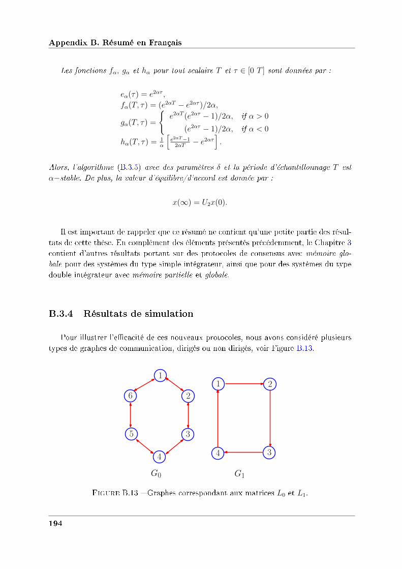
Appendix B. Résumé en Français
Les fonctions 𝑓𝛼, 𝑔𝛼 et ℎ𝛼 pour tout scalaire 𝑇 et 𝜏 ∈ [0 𝑇 ] sont données par :
𝑒𝛼(𝜏) = 𝑒2𝛼𝜏 ,
𝑓𝛼(𝑇, 𝜏) = (𝑒2𝛼𝑇 − 𝑒2𝛼𝜏 )/2𝛼,
𝑔𝛼(𝑇, 𝜏) =
𝑒2𝛼𝑇 (𝑒2𝛼𝜏 − 1)/2𝛼, if 𝛼 > 0
(𝑒2𝛼𝜏 − 1)/2𝛼, if 𝛼 < 0
ℎ𝛼(𝑇, 𝜏) = 1𝛼
[𝑒2𝛼𝑇−12𝛼𝑇
− 𝑒2𝛼𝜏].
Alors, l’algorithme (B.3.5) avec des paramètres 𝛿 et la période d’échantillonnage 𝑇 est
𝛼−stable. De plus, la valeur d’équilibre/d’accord est donnée par :
𝑥(∞) = 𝑈2𝑥(0).
Il est important de rappeler que ce résumé ne contient qu'une petite partie des résul-tats de cette thèse. En complément des éléments présentés précédemment, le Chapitre 3contient d'autres résultats portant sur des protocoles de consensus avec mémoire glo-
bale pour des systèmes du type simple intégrateur, ainsi que pour des systèmes du typedouble intégrateur avec mémoire partielle et globale.
B.3.4 Résultats de simulation
Pour illustrer l'ecacité de ces nouveaux protocoles, nous avons considéré plusieurstypes de graphes de communication, dirigés ou non dirigés, voir Figure B.13.
1
2
3
4
5
6
G0 G1
1 2
34
Figure B.13 Graphes correspondant aux matrices 𝐿0 et 𝐿1.
194
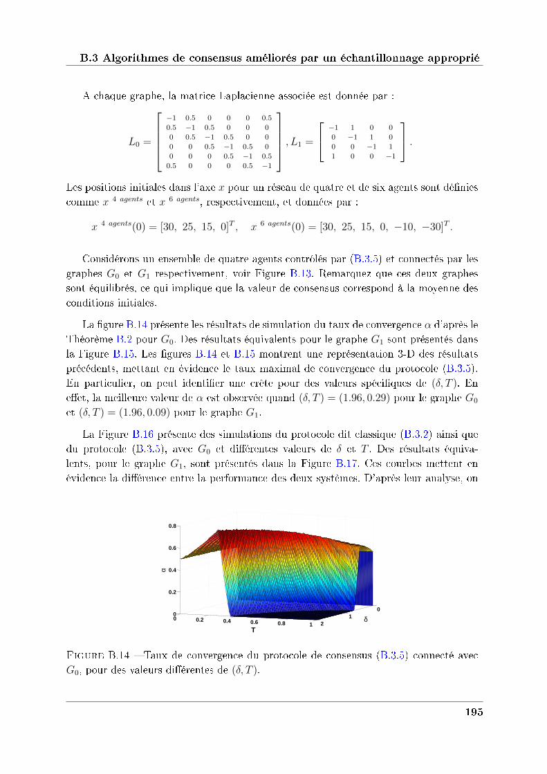
B.3 Algorithmes de consensus améliorés par un échantillonnage approprié
A chaque graphe, la matrice Laplacienne associée est donnée par :
𝐿0 =
⎡⎢⎢⎢⎣−1 0.5 0 0 0 0.5
0.5 −1 0.5 0 0 0
0 0.5 −1 0.5 0 0
0 0 0.5 −1 0.5 0
0 0 0 0.5 −1 0.5
0.5 0 0 0 0.5 −1
⎤⎥⎥⎥⎦ , 𝐿1 =
⎡⎣ −1 1 0 0
0 −1 1 0
0 0 −1 1
1 0 0 −1
⎤⎦ .Les positions initiales dans l'axe 𝑥 pour un réseau de quatre et de six agents sont déniescomme 𝑥 4 𝑎𝑔𝑒𝑛𝑡𝑠 et 𝑥 6 𝑎𝑔𝑒𝑛𝑡𝑠, respectivement, et données par :
𝑥 4 𝑎𝑔𝑒𝑛𝑡𝑠(0) = [30, 25, 15, 0]𝑇 , 𝑥 6 𝑎𝑔𝑒𝑛𝑡𝑠(0) = [30, 25, 15, 0, −10, −30]𝑇 .
Considérons un ensemble de quatre agents contrôlés par (B.3.5) et connectés par lesgraphes 𝐺0 et 𝐺1 respectivement, voir Figure B.13. Remarquez que ces deux graphessont équilibrés, ce qui implique que la valeur de consensus correspond à la moyenne desconditions initiales.
La gure B.14 présente les résultats de simulation du taux de convergence 𝛼 d'après leThéorème B.2 pour 𝐺0. Des résultats équivalents pour le graphe 𝐺1 sont présentés dansla Figure B.15. Les gures B.14 et B.15 montrent une représentation 3-D des résultatsprécédents, mettant en évidence le taux maximal de convergence du protocole (B.3.5).En particulier, on peut identier une crête pour des valeurs spéciques de (𝛿, 𝑇 ). Eneet, la meilleure valeur de 𝛼 est observée quand (𝛿, 𝑇 ) = (1.96, 0.29) pour le graphe 𝐺0
et (𝛿, 𝑇 ) = (1.96, 0.09) pour le graphe 𝐺1.
La Figure B.16 présente des simulations du protocole dit classique (B.3.2) ainsi quedu protocole (B.3.5), avec 𝐺0 et diérentes valeurs de 𝛿 et 𝑇 . Des résultats équiva-lents, pour le graphe 𝐺1, sont présentés dans la Figure B.17. Ces courbes mettent enévidence la diérence entre la performance des deux systèmes. D'après leur analyse, on
01
20 0.2 0.4 0.6 0.8 1
0
0.2
0.4
0.6
0.8
α
δT
Figure B.14 Taux de convergence du protocole de consensus (B.3.5) connecté avec𝐺0, pour des valeurs diérentes de (𝛿, 𝑇 ).
195
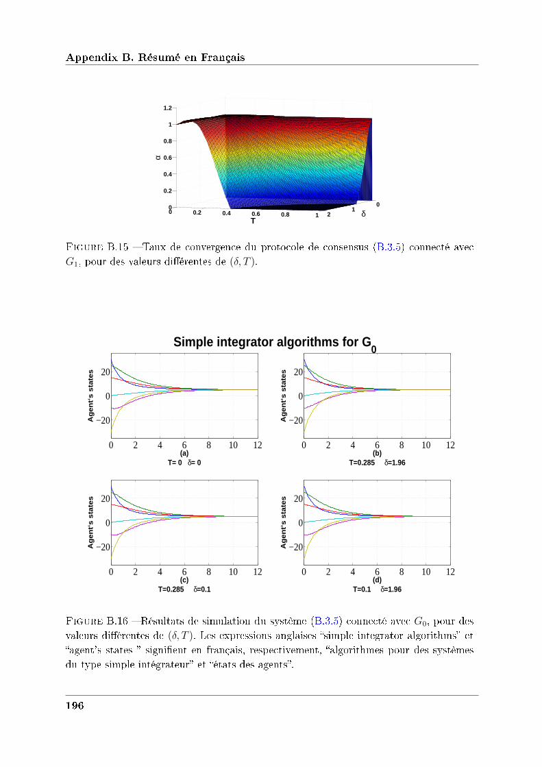
Appendix B. Résumé en Français
01
20 0.2 0.4 0.6 0.8 10
0.2
0.4
0.6
0.8
1
1.2
T
α
Tδ
Figure B.15 Taux de convergence du protocole de consensus (B.3.5) connecté avec𝐺1, pour des valeurs diérentes de (𝛿, 𝑇 ).
0 2 4 6 8 10 12
−20
0
20
Ag
en
t‘s
sta
tes
(a)T= 0 δ= 0
0 2 4 6 8 10 12
−20
0
20
Ag
en
t‘s
sta
tes
(b)T=0.285 δ=1.96
0 2 4 6 8 10 12
−20
0
20
Ag
en
t‘s
sta
tes
(c)T=0.285 δ=0.1
0 2 4 6 8 10 12
−20
0
20
Ag
en
t‘s
sta
tes
(d)T=0.1 δ=1.96
Simple integrator algorithms for G0
Figure B.16 Résultats de simulation du système (B.3.5) connecté avec 𝐺0, pour desvaleurs diérentes de (𝛿, 𝑇 ). Les expressions anglaises simple integrator algorithms etagent's states signient en français, respectivement, algorithmes pour des systèmesdu type simple intégrateur et états des agents.
196
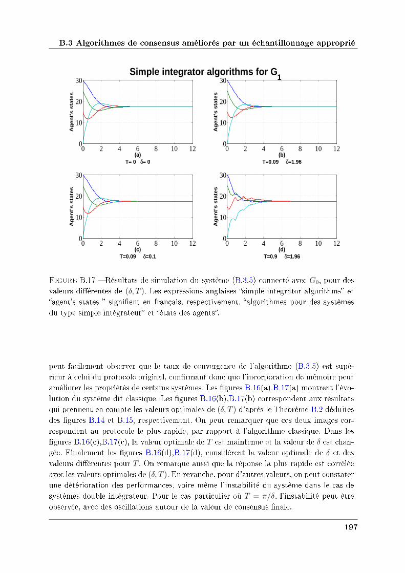
B.3 Algorithmes de consensus améliorés par un échantillonnage approprié
0 2 4 6 8 10 120
10
20
30
Ag
en
t‘s
sta
tes
(a)T= 0 δ= 0
0 2 4 6 8 10 120
10
20
30
Ag
en
t‘s
sta
tes
(b)T=0.09 δ=1.96
0 2 4 6 8 10 120
10
20
30
Ag
en
t‘s
sta
tes
(c)T=0.09 δ=0.1
0 2 4 6 8 10 120
10
20
30
Ag
en
t‘s
sta
tes
(d)T=0.9 δ=1.96
Simple integrator algorithms for G1
Figure B.17 Résultats de simulation du système (B.3.5) connecté avec 𝐺0, pour desvaleurs diérentes de (𝛿, 𝑇 ). Les expressions anglaises simple integrator algorithms etagent's states signient en français, respectivement, algorithmes pour des systèmesdu type simple intégrateur et états des agents.
peut facilement observer que le taux de convergence de l'algorithme (B.3.5) est supé-rieur à celui du protocole original, conrmant donc que l'incorporation de mémoire peutaméliorer les propriétés de certains systèmes. Les gures B.16(a),B.17(a) montrent l'évo-lution du système dit classique. Les gures B.16(b),B.17(b) correspondent aux résultatsqui prennent en compte les valeurs optimales de (𝛿, 𝑇 ) d'après le Theorème B.2 déduitesdes gures B.14 et B.15, respectivement. On peut remarquer que ces deux images cor-respondent au protocole le plus rapide, par rapport à l'algorithme classique. Dans lesgures B.16(c),B.17(c), la valeur optimale de 𝑇 est maintenue et la valeur de 𝛿 est chan-gée. Finalement les gures B.16(d),B.17(d), considèrent la valeur optimale de 𝛿 et desvaleurs diérentes pour 𝑇 . On remarque aussi que la réponse la plus rapide est corréléeavec les valeurs optimales de (𝛿, 𝑇 ). En revanche, pour d'autres valeurs, on peut constaterune détérioration des performances, voire même l'instabilité du système dans le cas desystèmes double intégrateur. Pour le cas particulier où 𝑇 = 𝜋/𝛿, l'instabilité peut êtreobservée, avec des oscillations autour de la valeur de consensus nale.
197
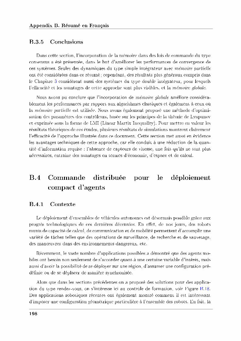
Appendix B. Résumé en Français
B.3.5 Conclusions
Dans cette section, l'incorporation de la mémoire dans des lois de commande du typeconsensus a été présentée, dans le but d'améliorer les performances de convergence deces systèmes. Seules des dynamiques du type simple intégrateur avec mémoire partielle
ont été considérées dans ce résumé ; cependant, des résultats plus généraux compris dansle Chapitre 3 considèrent aussi des systèmes du type double intégrateur, pour lesquelsl'ecacité et les avantages de cette approche sont plus visibles, et la mémoire globale.
Nous avons pu conclure que l'incorporation de mémoire globale améliore considéra-blement les performances par rapport aux algorithmes classiques et également à ceux oùla mémoire partielle est utilisée. Nous avons également proposé une méthode d'optimi-sation des paramètres des contrôleurs, basée sur les principes de la théorie de Lyapunovet exprimée sous la forme de LMI (Linear Martix Inequality). Pour mettre en valeur lesrésultats théoriques de ces études, plusieurs résultats de simulations montrent clairementl'ecacité de l'approche illustrée dans ce document. Cette section met aussi en évidenceles avantages techniques de cette approche, car elle conduit à une réduction de la quan-tité d'information requise : l'absence de capteurs de vitesse, une fois qu'ils ne sont plusnécessaires, entraîne des avantages en termes d'économie, d'espace et de calcul.
B.4 Commande distribuée pour le déploiement
compact d’agents
B.4.1 Contexte
Le déploiement d'ensembles de véhicules autonomes est désormais possible grâce auxprogrès technologiques de ces dernières décennies. En eet, de nos jours, des robotsmunis de capacité de calcul, de communication et de mobilité permettent d'accomplir unevariété de tâches telles que des opérations de surveillance, de recherche et de sauvetage,des man÷uvres dans des environnements dangereux, etc.
Récemment, le vaste nombre d'applications possibles a démontré que des agents mo-biles ont besoin non seulement de s'accorder quant à une certaine variable d'intérêt, maisaussi d'avoir la possibilité de se déployer sur une région, d'assumer une conguration pré-dénie ou de se déplacer de manière synchronisée.
Alors que dans les sections précédentes on a proposé des solutions pour des applica-tion du type rendez-vous, on s'intéresse ici au contrôle de formation, voir Figure B.18.Des applications robotiques récentes ont également montré comment il est intéressantd'imposer une conguration géométrique particulière à l'ensemble des robots. En fait, la
198
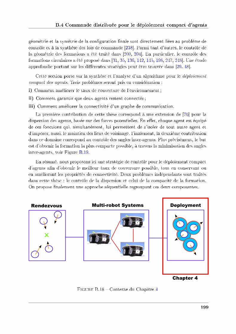
B.4 Commande distribuée pour le déploiement compact d’agents
géométrie et la symétrie de la conguration nale sont directement liées au problème decontrôle et à la synthèse des lois de commande [238]. Parmi tant d'autres, le contrôle dela géométrie des formations a été traité dans [200, 204]. En particulier, le contrôle desformations circulaires a été proposé dans [31, 35, 136, 142, 145, 198, 247, 248]. Une étudeapprofondie portant sur les diérentes stratégies peut être trouvée dans [29, 48].
Cette section porte sur la synthèse et l'analyse d'un algorithme pour le déploiementcompact des agents. Trois problèmes seront pris en considération :
i) Comment améliorer le taux de couverture de l'environnement ;
ii) Comment garantir que deux agents restent connectés ;
iii) Comment améliorer la connectivité d'un graphe de communication.
La première contribution de cette thèse correspond à une extension de [76] pour ladispersion des agents, basée sur des forces potentielles. En eet, chaque agent est équipéde ces fonctions qui, simultanément, lui permettent de s'isoler de tout autre agent etd'imposer, aussi, le maintien des liens de voisinage. Finalement, la deuxième contributiondans ce domaine correspond au contrôle des angles inter-agents. Plus précisément, le butest d'obtenir la formation la plus compacte possible, à travers la minimisation des anglesinter-agents, voir Figure B.19.
En résumé, nous proposons ici une stratégie de contrôle pour le déploiement compactd'agents an d'obtenir le meilleur taux de couverture possible, tout en conservant ouen améliorant les propriétés de connectivité. Deux problèmes indépendants sont traitésdans cette thèse : le contrôle de la dispersion et celui de la compacité de la formation.On propose nalement une approche séquentielle regroupant ces deux composantes.
Multi-robot Systems
x
Rendezvous Deployment
Chapter 4
Figure B.18 Contexte du Chapitre 4
199
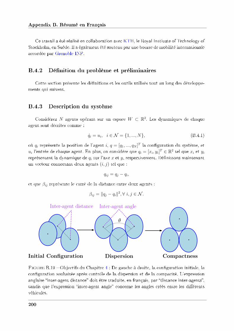
Appendix B. Résumé en Français
Ce travail a été réalisé en collaboration avec KTH, le Royal Institute of Technology ofStockholm, en Suède. Il a également été soutenu par une bourse de mobilité internationaleaccordée par Grenoble INP.
B.4.2 Définition du problème et préliminaires
Cette section présente les dénitions et les outils utilisés tout au long des développe-ments qui suivent.
B.4.3 Description du système
Considérez 𝑁 agents opérant sur un espace 𝑊 ⊂ R2. Les dynamiques de chaqueagent sont décrites comme :
𝑞𝑖 = 𝑢𝑖, 𝑖 ∈ 𝒩 = 1, ..., 𝑁, (B.4.1)
où 𝑞𝑖 représente la position de l'agent 𝑖, 𝑞 = [𝑞1, ..., 𝑞𝑁 ]𝑇 la conguration du système, et𝑢𝑖 l'entrée de chaque agent. En plus, on considère que 𝑞𝑖 = [𝑥𝑖, 𝑦𝑖]
𝑇 ∈ R2 tel que 𝑥𝑖 et 𝑦𝑖représentent la dynamique de 𝑞𝑖 sur l'axe 𝑥 et 𝑦, respectivement. Dénissons maintenantun vecteur connectant deux agents (𝑖, 𝑗) tel que :
𝑞𝑖𝑗 = 𝑞𝑗 − 𝑞𝑖,
et que 𝛽𝑖𝑗 représente le carré de la distance entre deux agents :
𝛽𝑖𝑗 = ‖𝑞𝑗 − 𝑞𝑖‖2, ∀ 𝑖, 𝑗 ∈ 𝒩 .
Initial Configuration CompactnessDispersion
θ
Inter-agent angleInter-agent distance
Figure B.19 Objectifs du Chapitre 4 : De gauche à droite, la conguration initiale, laconguration souhaitée après contrôle de la dispersion et de la compacité. L'expressionanglaise inter-agent distance doit être traduite, en français, par distance inter-agents,tandis que l'expression inter-agent angle concerne les angles créés entre les diérentsvéhicules.
200
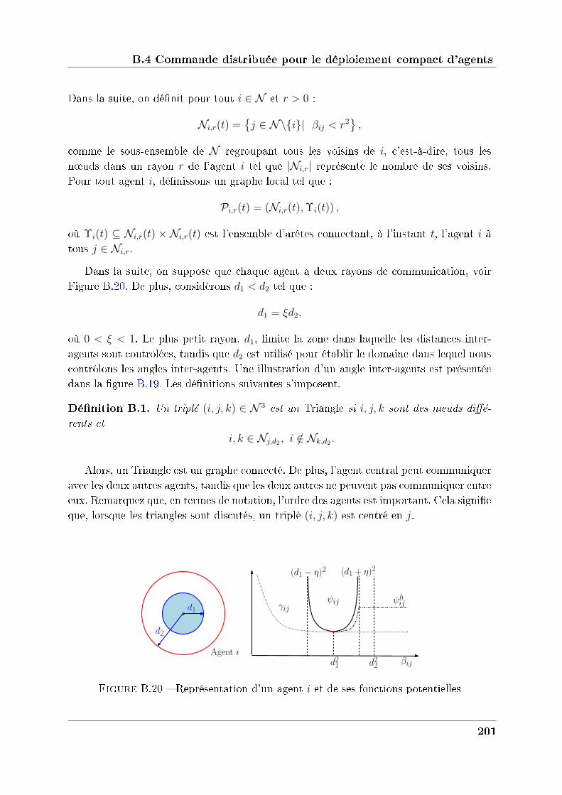
B.4 Commande distribuée pour le déploiement compact d’agents
Dans la suite, on dénit pour tout 𝑖 ∈ 𝒩 et 𝑟 > 0 :
𝒩𝑖,𝑟(𝑡) =𝑗 ∈ 𝒩∖𝑖| 𝛽𝑖𝑗 < 𝑟2
,
comme le sous-ensemble de 𝒩 regroupant tous les voisins de 𝑖, c'est-à-dire, tous lesn÷uds dans un rayon 𝑟 de l'agent 𝑖 tel que |𝒩𝑖,𝑟| représente le nombre de ses voisins.Pour tout agent 𝑖, dénissons un graphe local tel que :
𝒫𝑖,𝑟(𝑡) = (𝒩𝑖,𝑟(𝑡),Υ𝑖(𝑡)) ,
où Υ𝑖(𝑡) ⊆ 𝒩𝑖,𝑟(𝑡) × 𝒩𝑖,𝑟(𝑡) est l'ensemble d'arêtes connectant, à l'instant 𝑡, l'agent 𝑖 àtous 𝑗 ∈ 𝒩𝑖,𝑟.
Dans la suite, on suppose que chaque agent a deux rayons de communication, voirFigure B.20. De plus, considérons 𝑑1 < 𝑑2 tel que :
𝑑1 = 𝜉𝑑2,
où 0 < 𝜉 < 1. Le plus petit rayon, 𝑑1, limite la zone dans laquelle les distances inter-agents sont contrôlées, tandis que 𝑑2 est utilisé pour établir le domaine dans lequel nouscontrôlons les angles inter-agents. Une illustration d'un angle inter-agents est présentéedans la gure B.19. Les dénitions suivantes s'imposent.
Définition B.1. Un triplé (𝑖, 𝑗, 𝑘) ∈ 𝒩 3 est un Triangle si 𝑖, 𝑗, 𝑘 sont des nœuds diffé-
rents et
𝑖, 𝑘 ∈ 𝒩𝑗,𝑑2 , 𝑖 /∈ 𝒩𝑘,𝑑2 .
Alors, un Triangle est un graphe connecté. De plus, l'agent central peut communiqueravec les deux autres agents, tandis que les deux autres ne peuvent pas communiquer entreeux. Remarquez que, en termes de notation, l'ordre des agents est important. Cela signieque, lorsque les triangles sont discutés, un triplé (𝑖, 𝑗, 𝑘) est centré en 𝑗.
γij
βijd21
(d1 − η)2 (d1 + η)2
ψijd1
Agent id22
ψhijd1
d2
Figure B.20 Représentation d'un agent 𝑖 et de ses fonctions potentielles
201
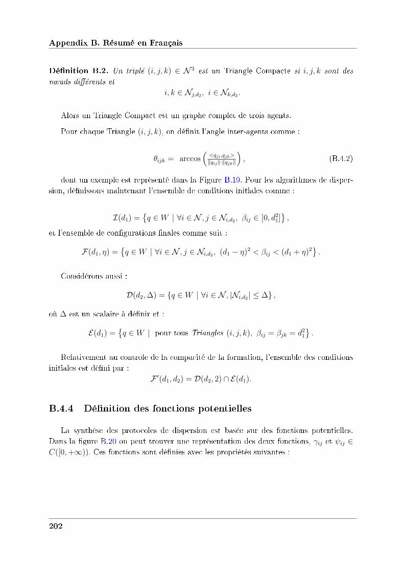
Appendix B. Résumé en Français
Définition B.2. Un triplé (𝑖, 𝑗, 𝑘) ∈ 𝒩 3 est un Triangle Compacte si 𝑖, 𝑗, 𝑘 sont des
nœuds différents et
𝑖, 𝑘 ∈ 𝒩𝑗,𝑑2 , 𝑖 ∈ 𝒩𝑘,𝑑2 .
Alors un Triangle Compact est un graphe complet de trois agents.
Pour chaque Triangle (𝑖, 𝑗, 𝑘), on dénit l'angle inter-agents comme :
𝜃𝑖𝑗𝑘 = arccos(<𝑞𝑗𝑖,𝑞𝑗𝑘>
‖𝑞𝑖𝑗‖·‖𝑞𝑗𝑘‖
), (B.4.2)
dont un exemple est représenté dans la Figure B.19. Pour les algorithmes de disper-sion, dénissons maintenant l'ensemble de conditions initiales comme :
ℐ(𝑑1) =𝑞 ∈ 𝑊 | ∀𝑖 ∈ 𝒩 , 𝑗 ∈ 𝒩𝑖,𝑑2 , 𝛽𝑖𝑗 ∈ ]0, 𝑑21]
,
et l'ensemble de congurations nales comme suit :
ℱ(𝑑1, 𝜂) =𝑞 ∈ 𝑊 | ∀𝑖 ∈ 𝒩 , 𝑗 ∈ 𝒩𝑖,𝑑2 , (𝑑1 − 𝜂)2 < 𝛽𝑖𝑗 < (𝑑1 + 𝜂)2
.
Considérons aussi :
𝒟(𝑑2,∆) = 𝑞 ∈ 𝑊 | ∀𝑖 ∈ 𝒩 , |𝒩𝑖,𝑑2| ≤ ∆ ,
où ∆ est un scalaire à dénir et :
ℰ(𝑑1) =𝑞 ∈ 𝑊 | pour tous Triangles (𝑖, 𝑗, 𝑘), 𝛽𝑖𝑗 = 𝛽𝑗𝑘 = 𝑑21
.
Relativement au contrôle de la compacité de la formation, l'ensemble des conditionsinitiales est déni par :
ℱ ′(𝑑1, 𝑑2) = 𝒟(𝑑2, 2) ∩ ℰ(𝑑1).
B.4.4 Définition des fonctions potentielles
La synthèse des protocoles de dispersion est basée sur des fonctions potentielles.Dans la gure B.20 on peut trouver une représentation des deux fonctions, 𝛾𝑖𝑗 et 𝜓𝑖𝑗 ∈𝐶([0,+∞)). Ces fonctions sont dénies avec les propriétés suivantes :
202
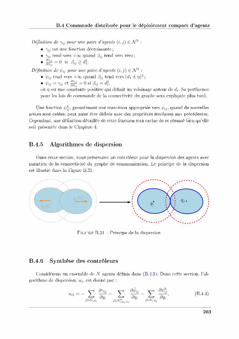
B.4 Commande distribuée pour le déploiement compact d’agents
Définition de 𝛾𝑖𝑗 pour une paire d’agents (𝑖, 𝑗) ∈ 𝒩 2 :
∙ 𝛾𝑖𝑗 est une fonction décroissante ;∙ 𝛾𝑖𝑗 tend vers +∞ quand 𝛽𝑖𝑗 tend vers zéro ;∙ 𝜕𝛾𝑖𝑗
𝜕𝛽𝑖𝑗= 0 si 𝛽𝑖𝑗 ≥ 𝑑21.
Définition de 𝜓𝑖𝑗 pour une paire d’agents (𝑖, 𝑗) ∈ 𝒩 2 :
∙ 𝜓𝑖𝑗 tend vers +∞ quand 𝛽𝑖𝑗 tend vers (𝑑1 ± 𝜂)2 ;∙ 𝜓𝑖𝑗 = 𝛾𝑖𝑗 et
𝜕𝛾𝑖𝑗𝜕𝛽𝑖𝑗
= 0 si 𝛽𝑖𝑗 = 𝑑21.où 𝜂 est une constante positive qui dénit un voisinage autour de 𝑑1. Sa pertinencepour les lois de commande de la connectivité du graphe sera expliquée plus tard.
Une fonction 𝜓ℎ𝑖𝑗, garantissant une transition appropriée vers 𝜓𝑖𝑗, quand de nouvellesarêtes sont créées, peut aussi être dénie avec des propriétés similaires aux précédentes.Cependant, une dénition détaillée de cette fonction sera exclue de ce résumé bien qu'ellesoit présentée dans le Chapitre 4.
B.4.5 Algorithmes de dispersion
Dans cette section, nous présentons un contrôleur pour la dispersion des agents avecmaintien de la connectivité du graphe de communication. Le principe de la dispersionest illustré dans la Figure B.21.
qi(0)qjqi
qj(0)
Figure B.21 Principe de la dispersion
B.4.6 Synthèse des contrôleurs
Considérons un ensemble de 𝑁 agents dénis dans (B.4.1). Dans cette section, l'al-gorithme de dispersion, 𝑢1, est donné par :
𝑢𝑖1 = −∑
𝑗∈𝒩𝑖,𝑑1
𝜕𝛾𝑖𝑗𝜕𝑞𝑖
−∑
𝑗∈𝒩ℎ𝑖,𝑑1+𝜂
𝜕𝜓𝑖𝑗𝜕𝑞𝑖
−∑
𝑗∈𝒩𝑖,𝑑2
𝜕𝜓ℎ𝑖𝑗𝜕𝑞𝑖
, (B.4.3)
203
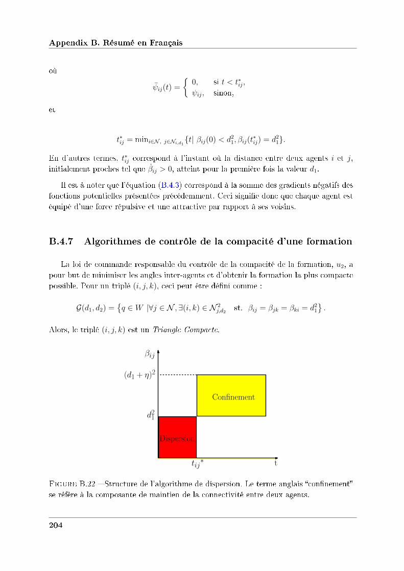
Appendix B. Résumé en Français
où
𝜓𝑖𝑗(𝑡) =
0, si 𝑡 < 𝑡*𝑖𝑗,
𝜓𝑖𝑗, sinon,
et
𝑡*𝑖𝑗 = min𝑖∈𝒩 , 𝑗∈𝒩𝑖,𝑑1𝑡| 𝛽𝑖𝑗(0) < 𝑑21, 𝛽𝑖𝑗(𝑡
*𝑖𝑗) = 𝑑21.
En d'autres termes, 𝑡*𝑖𝑗 correspond à l'instant où la distance entre deux agents 𝑖 et 𝑗,initialement proches tel que 𝑖𝑗 > 0, atteint pour la première fois la valeur 𝑑1.
Il est à noter que l'équation (B.4.3) correspond à la somme des gradients négatifs desfonctions potentielles présentées précédemment. Ceci signie donc que chaque agent estéquipé d'une force répulsive et une attractive par rapport à ses voisins.
B.4.7 Algorithmes de contrôle de la compacité d’une formation
La loi de commande responsable du contrôle de la compacité de la formation, 𝑢2, apour but de minimiser les angles inter-agents et d'obtenir la formation la plus compactepossible. Pour un triplé (𝑖, 𝑗, 𝑘), ceci peut être déni comme :
𝒢(𝑑1, 𝑑2) =𝑞 ∈ 𝑊 |∀𝑗 ∈ 𝒩 ,∃(𝑖, 𝑘) ∈ 𝒩 2
𝑗,𝑑2st. 𝛽𝑖𝑗 = 𝛽𝑗𝑘 = 𝛽𝑘𝑖 = 𝑑21
.
Alors, le triplé (𝑖, 𝑗, 𝑘) est un Triangle Compacte.
Dispersion
Confinement
tij∗ t
Confinement
βij
d21
(d1 + η)2
Figure B.22 Structure de l'algorithme de dispersion. Le terme anglais connementse réfère à la composante de maintien de la connectivité entre deux agents.
204
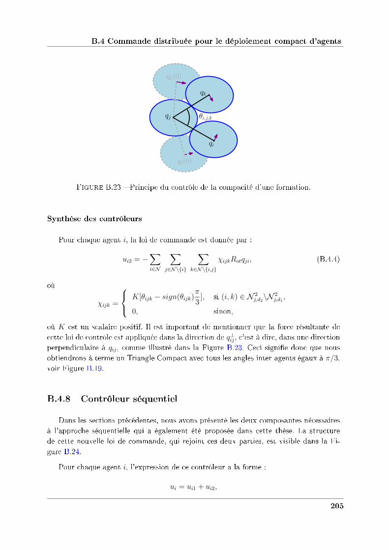
B.4 Commande distribuée pour le déploiement compact d’agents
qj
qk(0)
qi(0)
θi,j,k
qk
qi
Figure B.23 Principe du contrôle de la compacité d'une formation.
Synthèse des contrôleurs
Pour chaque agent 𝑖, la loi de commande est donnée par :
𝑢𝑖2 = −∑𝑖∈𝒩
∑𝑗∈𝒩∖𝑖
∑𝑘∈𝒩∖𝑖,𝑗
𝜒𝑖𝑗𝑘𝑅𝑜𝑡𝑞𝑗𝑖, (B.4.4)
où
𝜒𝑖𝑗𝑘 =
⎧⎨⎩ 𝐾[𝜃𝑖𝑗𝑘 − 𝑠𝑖𝑔𝑛(𝜃𝑖𝑗𝑘)𝜋
3], si (𝑖, 𝑘) ∈ 𝒩 2
𝑗,𝑑2∖𝒩 2
𝑗,𝑑1,
0, sinon,
où 𝐾 est un scalaire positif. Il est important de mentionner que la force résultante decette loi de contrôle est appliquée dans la direction de 𝑞⊥𝑖𝑗 , c'est à dire, dans une directionperpendiculaire à 𝑞𝑖𝑗, comme illustré dans la Figure B.23. Ceci signie donc que nousobtiendrons à terme un Triangle Compact avec tous les angles inter-agents égaux à 𝜋/3,voir Figure B.19.
B.4.8 Contrôleur séquentiel
Dans les sections précédentes, nous avons présenté les deux composantes nécessairesà l'approche séquentielle qui a également été proposée dans cette thèse. La structurede cette nouvelle loi de commande, qui rejoint ces deux parties, est visible dans la Fi-gure B.24.
Pour chaque agent 𝑖, l'expression de ce contrôleur a la forme :
𝑢𝑖 = 𝑢𝑖1 + 𝑢𝑖2,
205
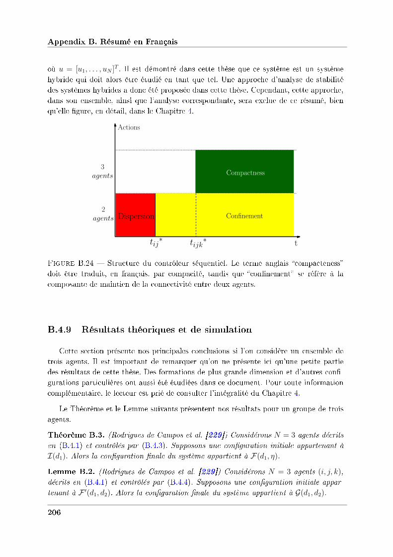
Appendix B. Résumé en Français
où 𝑢 = [𝑢1, . . . , 𝑢𝑁 ]𝑇 . Il est démontré dans cette thèse que ce système est un systèmehybride qui doit alors être étudié en tant que tel. Une approche d'analyse de stabilitédes systèmes hybrides a donc été proposée dans cette thèse. Cependant, cette approche,dans son ensemble, ainsi que l'analyse correspondante, sera exclue de ce résumé, bienqu'elle gure, en détail, dans le Chapitre 4.
Dispersion Confinement
tij∗ tijk
∗ t
Actions
2agents
3agents Compactness
Figure B.24 Structure du contrôleur séquentiel. Le terme anglais compactenessdoit être traduit, en français, par compacité, tandis que connement se réfère à lacomposante de maintien de la connectivité entre deux agents.
B.4.9 Résultats théoriques et de simulation
Cette section présente nos principales conclusions si l'on considère un ensemble detrois agents. Il est important de remarquer qu'on ne présente ici qu'une petite partiedes résultats de cette thèse. Des formations de plus grande dimension et d'autres con-gurations particulières ont aussi été étudiées dans ce document. Pour toute informationcomplémentaire, le lecteur est prié de consulter l'intégralité du Chapitre 4.
Le Théorème et le Lemme suivants présentent nos résultats pour un groupe de troisagents.
Théorème B.3. (Rodrigues de Campos et al. [229]) Considérons 𝑁 = 3 agents décrits
en (B.4.1) et contrôlés par (B.4.3). Supposons une configuration initiale appartenant à
ℐ(𝑑1). Alors la configuration finale du système appartient à ℱ(𝑑1, 𝜂).
Lemme B.2. (Rodrigues de Campos et al. [229]) Considérons 𝑁 = 3 agents (𝑖, 𝑗, 𝑘),
décrits en (B.4.1) et contrôlés par (B.4.4). Supposons une configuration initiale appar-
tenant à ℱ ′(𝑑1, 𝑑2). Alors la configuration finale du système appartient à 𝒢(𝑑1, 𝑑2).
206
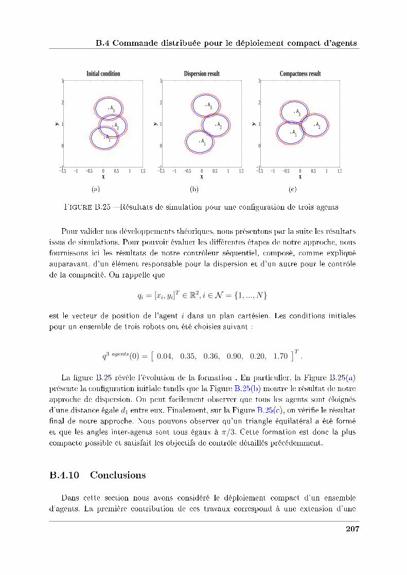
B.4 Commande distribuée pour le déploiement compact d’agents
−1.5 −1 −0.5 0 0.5 1 1.5−1
0
1
2
3
A1
y
x
Initial condition
A2
A3
(a)
−1.5 −1 −0.5 0 0.5 1 1.5−1
0
1
2
3
A1
x
Dispersion result
y A2
A3
(b)
−1.5 −1 −0.5 0 0.5 1 1.5−1
0
1
2
3
A1
x
Compactness result
y A2
A3
(c)
Figure B.25 Résultats de simulation pour une conguration de trois agents
Pour valider nos développements théoriques, nous présentons par la suite les résultatsissus de simulations. Pour pouvoir évaluer les diérentes étapes de notre approche, nousfournissons ici les résultats de notre contrôleur séquentiel, composé, comme expliquéauparavant, d'un élément responsable pour la dispersion et d'un autre pour le contrôlede la compacité. On rappelle que
𝑞𝑖 = [𝑥𝑖, 𝑦𝑖]𝑇 ∈ R2, 𝑖 ∈ 𝒩 = 1, ..., 𝑁
est le vecteur de position de l'agent 𝑖 dans un plan cartésien. Les conditions initialespour un ensemble de trois robots ont été choisies suivant :
𝑞3 𝑎𝑔𝑒𝑛𝑡𝑠(0) =[
0.04, 0.35, 0.36, 0.90, 0.20, 1.70]𝑇.
La gure B.25 révèle l'évolution de la formation . En particulier, la Figure B.25(a)présente la conguration initiale tandis que la Figure B.25(b) montre le résultat de notreapproche de dispersion. On peut facilement observer que tous les agents sont éloignésd'une distance égale 𝑑1 entre eux. Finalement, sur la Figure B.25(c), on vérie le résultatnal de notre approche. Nous pouvons observer qu'un triangle équilatéral a été forméet que les angles inter-agents sont tous égaux à 𝜋/3. Cette formation est donc la pluscompacte possible et satisfait les objectifs de contrôle détaillés précédemment.
B.4.10 Conclusions
Dans cette section nous avons considéré le déploiement compact d'un ensembled'agents. La première contribution de ces travaux correspond à une extension d'une
207
Appendix B. Résumé en Français
approche existante pour la dispersion, à laquelle on a ajouté une composante garantis-sant le maintien de la connectivité. Comme deuxième contribution de ce chapitre nousavons présenté une loi de commande qui permet le contrôle de la compacité de la for-mation. En eet, il semble qu'une approche qui permettrait d'agir directement sur lesangles inter-agents, contrôlant ainsi la connectivité du graphe de communication, n'a pasencore été proposée dans la littérature.
Finalement, nous avons présenté des résultats de simulation 2D pour une congura-tion de trois agents, comme un cas particulier de l'ensemble des congurations étudiéesdans cette thèse. Dans le cadre de recherches futures, nous avons l'intention de dévelop-per un algorithme généralisé pour toutes sortes de congurations initiales et de renforcerl'analyse de stabilité pour de tels cas.
B.5 Conclusions générales
Le but de cette section est de résumer les contributions de cette thèse et de présenterquelques perspectives pour de futures recherches. Cette thèse porte sur les stratégiesde contrôle distribué pour des systèmes multi-robots. Plus précisément, elle avance desrésultats pertinents concernant le contrôle d'un groupe de véhicules mobiles qui garan-tissent les meilleures propriétés de connectivité possibles. Un résumé des travaux de cettethèse gure dans la suite.
B.5.1 Algorithmes de consensus
Au cours d'une grande partie de cette thèse, une attention particulière est accordéeaux algorithmes de consensus pour des agents hétérogènes représentant, par exemple,diérents modèles ou générations de robots. Ces travaux ont été motivés par des appli-cations extrêmement exigeantes intégrant des agents hétérogènes tels que les opérationsde recherche, de sauvetage ou de surveillance, dans des congurations civiles ou mili-taires. Bien que plusieurs travaux considèrent des algorithmes de consensus pour desensembles homogènes d'agents, seuls quelques travaux étudient le cas des agents hétéro-gènes. De plus, les résultats qui en découlent présentent des inconvénients majeurs telsque les besoins de calcul ou la complexité.
Plus précisément, une stratégie, où le protocole de consensus est découplé du systèmed'origine, est présentée dans le Chapitre 2. En d'autres termes, nous attribuons à chaqueagent une variable de contrôle supplémentaire qui permet d'atteindre un consensus, touteen garantissant que la grandeur d'intérêt de chaque agent converge vers cette variablesupplémentaire. Le grand avantage de la méthode proposée réside dans une analysedécouplée entre les diérents composants du système. Par conséquent, il a été possible
208
B.5 Conclusions générales
d'étendre nos résultats à des situations plus complexes, en considérant, par exemple,des retards de communication ou des ltres distribués avec des références externes. Defutures recherches devront inclure l'étude des systèmes non linéaires ou des algorithmesde consensus en temps-ni. L'extension de méthodes et les outils d'analyse devront aussiêtre étudiés.
D'un autre côté, nous nous sommes intéressés à savoir s'il serait possible d'améliorerles propriétés de convergence des protocoles traditionnels. Dans le Chapitre 3, on proposed'incorporer de la mémoire dans de nouveaux protocoles pour des systèmes du typesimple et double intégrateur, c'est-à-dire, d'ajouter une composante échantillonnée del'état à la loi de commande. De plus, de la mémoire partielle et globale sont utilisées etles performances sont observées. L'analyse de stabilité de ces nouveaux algorithmes estbasée sur des conditions du type LMI. Cependant, la complexité d'une telle approcheaugmente considérablement pour les réseaux de grande dimension. Une évolution logiquedes résultats de cette thèse devrait inclure d'autres outils d'analyse, ainsi que l'étude descas asynchrones.
B.5.2 Déploiement compact d’agents
Dans le Chapitre 4 nous avons considéré le déploiement compact d'un ensembled'agents. La première contribution de ces travaux correspond à une extension d'une ap-proche existante pour la dispersion, à laquelle on a ajouté une composante qui garantitle maintien de la connectivité. La deuxième contribution comprend une loi de commandepermettant le contrôle de la compacité de la formation. Finalement, nous avons égale-ment présenté des résultats de simulation 2D pour une conguration de trois agents,comme un cas particulier de l'ensemble de congurations étudié dans cette thèse. Dansle cadre de recherches futures, nous avons l'intention de développer un algorithme géné-ralisé pour toutes sortes de congurations initiales et de renforcer l'analyse de stabilitépour de tels cas.
209
Bibliography
[1] Special issue on sensor networks and applications. Proceedings of the IEEE, 91(8),August 2003.
[2] Special issue on networking and information theory. IEEE Transactions on Infor-
mation Theory, 52(6), June 2006.
[3] H. Ando, Y. Oasa, Suzuki, and M. Yamashita. Distributed memoryless pointconvergence algorithm for mobile robots with limited visibility. IEEE Transactions
on Robotics and Automation, 15(5):818828, 1999.
[4] R. Aragues, G. Shi, D. V. Dimarogonas, C. Sagues, and K. H. Johansson. Dis-tributed algebraic connectivity estimation for adaptive event-triggered consensus.In American Control Conference, 2012.
[5] A. Arsie and E. Frazzoli. Ecient routing of multiple vehicles with no explicitcommunications. International Journal of Robust and Nonlinear Control, 18:154164, 2008.
[6] S. Bag, S. Spurgeon, and C. Edwards. Output feedback sliding mode design forlinear uncertain systems. IEEE Proceedings -Control Theory and Applications,144(3):209 216, may 1997.
[7] T. Balch and R. C. Arkin. Behavior-based formation control for multirobot teams.IEEE Transactions on Robotics and Automation, 14(6):926939, December 1998.
[8] M. Baseggio, A. Cenedese, P. Merlo, M. Pozzi, and L. Schenato. Distributedperimeter patrolling and tracking for camera networks. In 49𝑡ℎ IEEE Conference
on Decision and Control, Atlanta, USA, pages 20932098, 2010.
[9] M. Basiri, A. Bishop, and P. Jensfelt. Distributed control of triangular formationswith angle-only constraints. Systems & Control Letters, 59(2):147 154, 2010.
[10] M. Batalin and G. Sukhatme. Coverage, Exploration, and Deployment by a Mobile
Robot and Communication Network. Springer Berlin / Heidelberg, 2003.
[11] M. Batalin and G. Sukhatme. The analysis of an ecient algorithm for robot cov-erage and exploration based on sensor network deployment. In IEEE International
Conference on Robotics and Automation, pages 3478 3485, 2005.
210
Bibliography
[12] M. Batalin and G. Sukhatme. The design and analysis of an ecient local algo-rithm for coverage and exploration based on sensor network deployment. IEEE
Transactions on Robotics and Automation, 23(4):661675, 2007.
[13] D. Bauso, L. Giarre, and R. Pesenti. Attitude alignment of a team of UAVs underdecentralized information structure. In IEEE Conference on Control Applications,
Istanbul, Turkey, volume 1, pages 486 491, 2003.
[14] D. Bauso and R. Pesenti. Distributed consensus protocols for coordinating buyers.In 42𝑛𝑑 IEEE Conference on Decision and Control, Hawaii, pages 588592, 2003.
[15] R. W. Beard, J. Lawton, and F. Y. Hadaegh. A feedback architecture for formationcontrol. In American Control Conference, Chicago, IL, USA, volume 6, pages40874091, 2000.
[16] R. W. Beard, J. Lawton, and F. Y. Hadaegh. A coordination architecture forspacecraft formation control. IEEE Transactions on Control Systems Technology,9:777790, 2001.
[17] R. W. Beard, T. McLain, D. Nelson, D. Kingston, and D. Johanson. Decentralizedcooperative aerial surveillance using xed-wing miniature uavs. Proceedings of theIEEE, 94(7):1306 1324, 2006.
[18] C. Belta and V. Kumar. Abstraction and control for groups of robots. IEEE
Transactions on Robotics, 20(5):865875, 2004.
[19] M. Bennewitz, W. Burgard, and S. Thrun. Finding and optimizing solvable pri-ority schemes for decoupled path planning techniques for teams of mobile robots.Robotics and Autonomous Systems, 41(2-3):8999, 2002.
[20] D. P. Bertsekas and J. Tsitsiklis. Parallell and Distributed Computation. UpperSaddle River, 1989.
[21] S. Bhat and D. Bernstein. Continuous nite-time stabilization of the transla-tional and rotational double integrators. IEEE Transactions on Automatic Control,43(5):678 682, 1998.
[22] S. Bhat and D. Bernstein. Finite-time stability of contin- uous autonomous sys-tems. SIAM J. Control and Optimization, 38:751766, 2000.
[23] N. Biggs. Algebraic Graph Theory. Cambridge University Press, 1994.
[24] A. Bishop. A very relaxed control law for bearing-only triangular formation control.In 18𝑡ℎ IFAC World Congress, Milan, 2011.
[25] A. Bishop, I. Shames, and B. Anderson. Stabilization of rigid formations withdirection-only constraints. In 50𝑡ℎ IEEE Conference on Decision and Control and
European Control Conference, 2011.
[26] P.-A. Bliman and G. Ferrari-Trecate. Average consensus problems in networks ofagents with delayed communications. Automatica, 44:19851995, 2008.
211
Bibliography
[27] V. Borkar and P. Varaiya. Asymptotic agreement in distributed estimation. IEEETransactions on Automatic Control, 27(3):650655, 1982.
[28] M. Bowling and M. Veloso. Multiagent learning using a variable learning rate.Artificial Intelligence, 136:215250, 2002.
[29] L. Briñón-Arranz. Cooperative control design for a fleet of AUVs under communi-
cation constraints. PhD thesis, Université de Grenoble, Gipsa-Lab, 2011.
[30] L. Briñón-Arranz, A. Seuret, and C. Canudas-de-Wit. Translation control of aeet circular formation of AUVs under nite communication range. In 48𝑡ℎ IEEE
Conference on Decision and Control held jointly with the 28th Chinese Control
Conference, Shanghai, China, pages 83458350, 2009.
[31] L. Briñón-Arranz, A. Seuret, and C. Canudas-de-Wit. Contraction control of a eetcircular formation of auvs under limited communication range. In IEEE American
Control Conference, Baltimore, MD, USA, 2010.
[32] L. Briñón-Arranz, A. Seuret, and C. Canudas-de-Wit. General framework usingane transformations to formation control design. In 2𝑛𝑑 IFAC Workshop on
Distributed Estimation and Control in Networked Systems, Annecy, France, 2010.
[33] L. Briñón-Arranz, A. Seuret, and C. Canudas-de-Wit. Collaborative estimation ofgradient direction by a formation of auvs. In 5𝑡ℎ International ICST Conference
on Performance Evaluation Methodologies and Tools, 2011 Cachan, France, 2011.
[34] L. Briñón-Arranz, A. Seuret, and C. Canudas-de-Wit. Collaborative estimation ofgradient direction by a formation of auvs under communication constraints. In 50𝑡ℎ
IEEE Conference on Decision and Control, held jointly with the European Control
Conference, Orlando, FL, USA, 2011.
[35] L. Briñón-Arranz, A. Seuret, and C. Canudas-de-Wit. Elastic formation controlbased on ane transformations. In American Control Conference, San Francisco,
CA, USA, pages 39843989, 2011.
[36] A. M. Bruckstein, N. Cohen, and A. Efrat. Ants, crickets, and frogs in cyclicpursuit. Technical Report CIS 9105, Center for Intelligent Systems, Technion,Haifa, Israel, 1991.
[37] F. Bullo, J. Cortés, and S. Martínez. Distributed Control of Robotic Networks.
Applied Mathematics Series. Princeton University Press, 2009.
[38] K. Cai and H. Ishii. Quantized consensus and averaging on gossip digraphs. IEEETransactions on Automatic Control, 56(9):2087 2100, 2011.
[39] K. Cai and H. Ishii. Average consensus on arbitrary strongly connected digraphswith dynamic topologies. In American Control Conference, 2012.
[40] K. Cai and H. Ishii. Average consensus on general strongly connected digraphs.Automatica Submitted, 2012.
212
Bibliography
[41] C. Canudas de Wit, F. Garin, R. Fabbiano, P. Rouchon, and A. Rousseau. Sourcelocalization using poisson integral. In 3𝑡ℎ IFAC workshop on distributed estimation
and control in networked systems, 2012.
[42] M. Cao, A. S. Morse, and B. Anderson. Reaching a consensus in a dynamicallychanging environment-convergence rates, measurement delays and asynchronousevents. SIAM Journal on Control and Optimization, 47:601623, 2008.
[43] Z. Cao, L. Xie, B. Zhang, S. Wang, and M. Tan. Formation constrained multi-robotsystem in unknown environments. In IEEE International Conference on Robotics
and Automation, Taipei, Taiwan, volume 1, pages 735740, 2003.
[44] R. Carli and F. Bullo. Quantized coordination algorithms for rendezvous anddeployment. SIAM Journal on Control and Optimization, 48(3):12511274, 2009.
[45] J. Chen, D. Sun, J. Yang, and H. Chen. Leader-follower formation control ofmultiple non-holonomic mobile robots incorporating a receding-horizon scheme.The International Journal of Robotics Research, 29(6):727747, May 2010.
[46] J. Chen, D. Xie, and M. Yu. Consensus problem of networked multi-agent systemswith constant communication delay: stochastic switching topology case. Interna-tional Journal of Control-To appear, 85(9):12481262, 2012.
[47] T. Chen and B. Francis. Optimal sampled-data control systems. Springer-Verlag,Berlin, Germany, 1995.
[48] Y. Q. Chen and Z. Wang. Formation control: a review and a new considera-tion. In IEEE/RSJ International Conference on Intelligent Robots and Systems,
Edmonton, Alberta, Canada, pages 31813186, 2005.
[49] X. Cheng. On-line collision-free path planning for service and assembly tasks bya two-arm robot. In IEEE International Conference on Robotics and Automation,volume 2, pages 1523 1528 vol.2, may 1995.
[50] N. Chopra and M. W. Spong. Passivity-based control of multi-agent systems.Springer, 2006.
[51] N. Chopra and M. W. Spong. Output synchronization of nonlinear systems withrelative degree one. Recent. Adv. Learning Control, LNCIS371:5164, 2008.
[52] N. Chopra and M. W. Spong. On exponential synchronization of kuramoto oscil-lators. IEEE Transactions on Automatic Control, 54:353357, 2009.
[53] N. Chopra, D. Stipanovic, and M. W. Spong. On synchronization and collisionavoidance for mechanical systems. In American Control Conference,, pages 37133718, 2008.
[54] F. Chung. Spectral graph theory. In CBMS Regional Conference Series in Math-
ematics, 1997.
[55] T. Clutton-Brock, P. Brotherton, A. Russell, M. O'Riain, D. Gaynor, R. Kansky,A. Grin, M. Manse, L.Sharpe, G. McIlrath, T. Small, A. Moss, and S. Monfort.
213
Bibliography
Cooperation, control, and concession in meerkat groups. Science, 291(5503):478481, 2001.
[56] J. Cochran and M. Krsti¢. Source seeking with a nonholonomic unicycle withoutposition measurements and with tuning of angular velocity Part I: Stability anal-ysis. In 46𝑡ℎ IEEE Conference on Decision and Control, New Orleans, LA, USA,pages 60096016, 2007.
[57] J. Cochran, A. Siranosian, N. Ghods, and M. Krsti¢. Source seeking with a non-holonomic unicycle without position measurements and with tuning of angularvelocity Part II: Applications. In 46𝑡ℎ IEEE Conference on Decision and Control,
New Orleans, LA, USA, pages 19511956, 2007.
[58] L. Conradt and T. Roper. Group decision-making in animals. Nature, 421:155 158, 2003.
[59] L. Consolinia, F. Morbidib, D. Prattichizzo, and M. Tosques. On the control of aleader-follower formation of nonholonomic mobile robots. In 45𝑡ℎ IEEE Conference
on Decision and Control, San Diego, CA, USA, pages 59925997, 2006.
[60] L. Consolinia, F. Morbidib, D. Prattichizzo, and M. Tosques. Leader-follower for-mation control of nonholonomic mobile robots with input constraints. Automatica,44:13431349, 2008.
[61] J. Cortés and F. Bullo. Coordination and geometric optimization via distributeddynamical systems. SIAM Journal on Control and Optimization, 44(5):15431574,2005.
[62] J. Cortés, S. Martínez, and F. Bullo. Robust rendezvous for mobile autonomousagents via proximity graphs in arbitrary dimensions. IEEE Transactions on Auto-
matic Control, 51:12891298, 2006.
[63] J. Cortés, S. Martínez, T. Karata³, and F. Bullo. Coverage control for mobilesensing networks. IEEE Transactions on Robotics and Automation, 20(2):243255,2004.
[64] J. Cortés. Finite-time convergent gradient ows with applications to network con-sensus. Automatica, 42(11):1993 2000, 2006.
[65] I. D. Couzin, J. Krause, N. R. Franks, and S. A. Levin. Eective leadership anddecision-making in animal groups on the move. Nature, 433:513516, 2005.
[66] X. Cui, C. T. Hardin, R. K. Ragade, and A. S. Elmaghraby. A swarm approachfor emission sources localization. In 16th IEEE International Conference on Tools
with Artificial Intelligence, Boca Raton, FL, USA, pages 424430, 2004.
[67] T. B. Curtin, J. G. Bellingham, J. Catipovic, and D. Webb. Autonomous oceano-graphic sampling networks. Oceanography, 6(3):8694, 1993.
[68] P. Davidsson. Agent based social simulation: A computer science view. Journal
of Artificial Societies and Social Simulation, 5(1), 2002.
214
Bibliography
[69] G. de Castro and F. Paganini. Convex synthesis of controllers for consensus. InAmerican Control Conference, volume 6, pages 4933 4938, 2004.
[70] M. Defoort, T. Floquet, A. Kökösy, and W. Perruquetti. Sliding-mode formationcontrol for cooperative autonomous mobile robots. IEEE Transactions on Indus-
trial Electronics, 55:39443953, 2008.
[71] M. Defoort, A. Kokosy, T. Floquet, W. Perruquettic, and J. Palos. Motion planningfor cooperative unicycle-type mobile robots with limited sensing ranges: A dis-tributed receding horizon approach. Robotics and Autonomous Systems, 57:10941106, 2009.
[72] J. P. Desai, J. Ostrowski, and V. Kumar. Controlling formations of multiple mobilerobots. In IEEE International Conference on Robotics and Automation, Leuven,
Belgium, volume 4, pages 28642869, 1998.
[73] D. V. Dimarogonas and K. J. Kyriakopoulos. An inverse agreement control strategywith application to swarm dispersion. In 46𝑡ℎ IEEE Conference on Decision and
Control, pages 6148 6153, 2007.
[74] D. V. Dimarogonas and K. J. Kyriakopoulos. On the rendezvous problem formultiple nonholonomic agents. IEEE Transactions on Automatic Control, 52:916922, 2007.
[75] D. V. Dimarogonas and K. J. Kyriakopoulos. A connection between formationinfeasibility and velocity alignment in kinematic multi-agent systems. Automatica,44:26482654, 2008.
[76] D. V. Dimarogonas and K. J. Kyriakopoulos. Inverse agreement protocols withapplication to distributed multi-agent dispersion. IEEE Transactions on Automatic
Control, 54(3):657 663, 2009.
[77] D. V. Dimarogonas, S. G. Loizou, K. J. Kyriakopoulos, and M. Zavlanos. Afeedback stabilization and collision avoidance scheme for multiple independent non-point agents. Automatica, 42:229243, 2006.
[78] K. Do. Flocking for multiple elliptical agents with limited communication ranges.Asian Journal of Control, 27(5):931942, 2011.
[79] K. Do and M. Lau. Practical formation control of multiple unicycle-type mobilerobots with limited sensing ranges. Journal of Intelligent & Robotic Systems,64:245275, 2011.
[80] A. Doniec, N. Bouraqadi, M. Defoort, V. T. Le, and S. Stinckwich. Distributedconstraint reasoning applied to multi-robot exploration. In 21𝑠𝑡 IEEE International
Conference on Tools with Artificial Intelligence, Newark, NJ, USA, pages 159166,2009.
[81] D. D. Dudenhoeer and M. P. Jones. A formation behavior for large-scale micro-robot force deployement. In 32𝑛𝑑 Conference on Winter simulation, Orlando, FL,
USA, pages 972982, 2000.
215
Bibliography
[82] C. Edwards and S. K. Spurgeon. Sliding mode stabilization of uncertain systemsusing only output information. International Journal of Control, 62(5):11291144,1995.
[83] C. Edwards and S. K. Spurgeon. Sliding Mode Control: Theory and Applications.London, U.K.: Taylor and Francis, 1998.
[84] D. B. Edwards, T. A. Bean, D. L. Odell, and M. J. Anderson. A leader-followeralgorithm for multiple auv formations. IEEE/OES Autonomous Underwater Ve-
hicles, pages 4046, 2004.
[85] M. Egerstedt and X. Hu. Formation constrained multi-agent control. IEEE Trans-
actions on Robotics and Automation, 17:947951, 2001.
[86] F. Fagnani and S. Zampieri. Average consensus with packet drop communication.In 45𝑡ℎ IEEE Conference on Decision and Control, 2006.
[87] Y. Fan, G. Feng, and Y. Wang. Combination framework of rendezvous algorithmfor multi-agent systems with limited sensing ranges. Asian Journal of Control,13(2):283294, 2011.
[88] J. A. Fax and R. M. Murray. Graph laplacians and stabilization of vehicle forma-tions. In 15𝑡ℎ IFAC World Conference, Barcelona, Spain, July 2002.
[89] J. A. Fax and R. M. Murray. Information ow and cooperative control of vehicleformations. IEEE Transactions on Automatic Control, 49:14651476, 2004.
[90] J. Feddema, C. Lewis, and D. Schoenwald. Decentralized control of cooperativerobotic vehicles: theory and application. IEEE Transactions on Robotics and
Automation, 18(5):852 864, 2002.
[91] X. Feng and W. Long. Reaching agreement in nite time via continuous local statefeedback. In Chinese Control Conference, 2007.
[92] J. Ferber. Multi-Agent System: An Introduction to Distributed Artificial Intelli-
gence. Addison Wesley Longman, 1999.
[93] C. Ferrari, E. Pagello, J. Ota, and T. Arai. Multirobot motion coordination inspace and time. Robotics and Autonomous Systems, 25:219229, 1998.
[94] M. Fiedler. Algebraic connectivity of graphs. Number no. 2. Czechoslovak Mathe-matical Journal, 1973.
[95] T. Fraichard. Trajectory planning in dynamic workspace: a state-time space ap-proach. Advanced Robotics, 13(6-8):7594, 1999.
[96] E. Frazzoli, M. A. Dahleh, and E. Feron. Robust hybrid control for autonomousvehicle motion planning. In 39𝑡ℎ IEEE Conference on Decision and Control, pages821826, 2000.
[97] E. Fridman. A rened input delay approach to sampled-data control. Automatica,46(2):421427, 2010.
216
Bibliography
[98] E. Fridman, A. Seuret, and J.-P. Richard. Robust sampled-data stabilization oflinear systems: An input delay approach. Automatica, 40(8):11411446, 2004.
[99] A. Frommer and D. B. Szyld. On asynchronous iterations. Journal of Computa-
tional and Applied Mathematics, 123(1):201216, 2000.
[100] H. Fujioka. Stability analysis of systems with aperiodic sample-and-hold devices.Automatica, 45(3):771775, 2009.
[101] A. Ganguli, J. Cortés, and F. Bullo. Distributed deployment of asynchronousguards in art galleries. In American Control Conference, pages 14161421, 2006.
[102] V. Gazi and K. M. Passino. Stability analysis of swarms. IEEE Transactions on
Automatic Control, 48(4):692697, 2003.
[103] S. S. Ge, C.-H. Fua, and K. W. Lim. Multi-robot formations: queues and articialpotential trenches. In IEEE International Conference on Robotics and Automation,
New Orleans, LA, USA, volume 4, pages 33453350, 2004.
[104] R. Ghabcheloo, A. Pascoal, C. Silvestre, and I. Kaminer. Coordinated path follow-ing control of multiple wheeled robots with directed communication links. In 44𝑡ℎ
IEEE Conference on Decision and Control, and the European Control Conference
2005, Seville, Spain, 2005.
[105] S. Glavaski, M. Chaves, R. Day, P. Nag, A. Williams, and W. Zhang. Vehicle net-works: achieving regular formation. In American Control Conference, Minneapolis,
MN, USA, volume 5, pages 40954100, 2003.
[106] C. Godsil and G. Royle. Algebraic Graph Theory, volume 207. Springer-Verlag,2001.
[107] R. Goebel, R. Sanfelice, and A. Teel. Hybrid dynamical systems. IEEE Control
Systems Magazine, 29(2):28 93, 2009.
[108] M. F. Z. Goldgeier and P. S. Krishnaprasad. Control of small formations usingshape coordinates. In IEEE International Conference on Robotics and Automation,
Taipei, Taiwan, pages 25102515, 2003.
[109] M. Greytak and F. S. Hover. Motion planning with an analytic risk cost forholonomic vehicles. In 48𝑡ℎ IEEE Conference on Decision and Control held jointly
with the 28th Chinese Control Conference, Shanghai, China, 2009.
[110] K. Gu, V.-L. Kharitonov, and J. Chen. Stability of time-delay systems. Birkhauser,2003.
[111] V. Gupta, B. Hassibi, and R. M. Murray. Stability analysis of stochastically vary-ing formations of dynamic agents. In 42𝑛𝑑 IEEE Conference on Decision and
Control,Maui, Hawai, pages 504509, 2003.
[112] H. Hao and P. Barooah. Improving convergence rate of distributed consensusthrough asymmetric weights. In American Control Conference, 2012.
217
Bibliography
[113] Y. Hatano and M. Mesbahi. Agreement over random networks. In 43𝑟𝑑 IEEE
Conference on Decision and Control, pages 2010 2015, 2004.
[114] Y. Hatano and M. Mesbahi. Agreement over random networks. IEEE Transactions
on Automatic Control, 50(7):16071613, 2004.
[115] B. Hayes-Roth. An architecture for adaptive intelligent systems. Artificial Intelli-gence, 72(1):329 365, 1995.
[116] D. Helbing. Trac and related self-driven many-particle systems. Rev. Mod. Phys.,73:10671141, 2001.
[117] J. M. Hendrickx. Graphs and Networks for the Analysis of Autonomous Agent
Systems. PhD thesis, Université catholique de Louvain, Ecole Polytechnique deLouvain, Département d'Ingénierie Mathématique, 2008.
[118] S. Hernandez and D. A. Paley. Three-dimensional motion coordination in a time-invariant oweld. In 48𝑡ℎ IEEE Conference on Decision and Control held jointly
with the 28th Chinese Control Conference, Shanghai, China, pages 70437048,2009.
[119] J. Hespanha. Uniform stability of switched linear systems: extensions of lasalle'sinvariance principle. IEEE Transactions on Automatic Control, 49(4):470 482,2004.
[120] J. Hespanha, P. Naghshtabrizi, and Y. Xu. A survey of recent results in networkedcontrol systems. Proceedings of IEEE, 95(1):138 162, 2007.
[121] L. Hetel. Robust stability and control of switched linear systems. Phd thesis, InstitutNational Polytechnique de Lorraine - INPL, Nancy France, 2007.
[122] L. Hetel, J. Daafouz, and C. Iung. Stabilization of arbitrary switched linear systemswith unknown time-varying delays. IEEE Transactions on Automatic Control,51(10):16681674, 2006.
[123] Y. Hong, J. Huang, and Y. Xu. On an output feedback nite-time stabilizationproblem. IEEE Transactions on Automatic Control, 46(2):305 309, 2001.
[124] Y. Hong and Z.-P. Jiang. Finite-time stabilization of nonlinear systems withparametric and dynamic uncertainties. IEEE Transactions on Automatic Control,51(12):1950 1956, 2006.
[125] T.-y. Huang, X.-b. Chen, W.-b. Xu, and W. Wang. A self-organized approach tocollaborative handling of multi-robot systems. In Advances in Swarm Intelligence,volume 6729 of Lecture Notes in Computer Science, pages 8290. Springer Berlin/ Heidelberg, 2011.
[126] A. Isidori. Nonlinear Control Systems. Springer, 1995.
[127] A. Jadbabaie, J. Lin, and A. S. Morse. Coordination of groups of mobile au-tonomous agents using nearest neighbor rules. IEEE Transactions on Automatic
Control, 48(6):9881001, June 2003.
218
Bibliography
[128] A. Jadbabaie, J. Lin, and A. S. Morse. Coordination of groups of mobile au-tonomous agents using nearest neighbor rules. IEEE Transactions on Automatic
Control, 48(6):9881001, 2003.
[129] M. Ji and M. Egerstedt. Distributed coordination control of multi-agent systemswhile preserving connectedness. IEEE Transactions on Robotics, 23(4):693703,2007.
[130] U. Jönsson and C.-Y. Kao. Consensus of heterogeneous linear agents applied toa formation control problem. In 49𝑡ℎ IEEE Conference on Decision and Control,pages 6902 6907, 2010.
[131] E. W. Justh and P. S. Krishnaprasad. Equilibria and steering laws for planarformations. Systems & Control Letters, 52(1):2538, 2004.
[132] A. Kashyap, T. Basar, and R. Srikant. Quantized consensus. Automatica,43(7):11921203, 2007.
[133] H. Kim, H. Shim, and J. H. Seo. Output consensus of heterogeneous uncertainlinear multi-agent systems. IEEE Transactions on Automatic Control, 56(1):200206, 2011.
[134] T.-H. Kim and T. Sugie. Cooperative control for target-capturing task based on acyclic pursuit strategy. Automatica, 43:14261431, 2007.
[135] E. Klavins, R. Ghrist, and D. Lipsky. A grammatical approach to self-organizingrobotic systems. IEEE Transactions on Automatic Control, 51(6):949962, 2006.
[136] D. J. Klein and K. A. Morgansen. Controlled collective motion for trajectorytracking. In American Control Conference, Minneapolis, MN, USA, pages 52695275, June 2006.
[137] D. Kostic, S. Adinandra, J. Caarls, N. V. D. Wouw, and H. Nijmeijer. Collision-free tracking control of unicycle mobile robots. In 48𝑡ℎ IEEE Conference on Deci-
sion and Control held jointly with the 28th Chinese Control Conference, Shanghai,
China, 2009.
[138] M. Krsti¢ and H.-H. Wang. Stability of extremum seeking feedback for generalnonlinear dynamic systems. Automatica, 36:595601, 2000.
[139] Y. Kuramoto. Self-entrainment of a population of coupled non-linear oscillators. InInternational Symposium on Mathematical Problems in Theoretical Physics, vol-ume 39 of Lecture Notes in Physics, pages 420422. Springer Berlin / Heidelberg,1975.
[140] Y. Kuramoto. Collective synchronization of pulse-coupled oscillators and excitableunits. Physica D: Nonlinear Phenomena, 50:1530, 1991.
[141] A. Kwok and S. Martínez. Unicycle coverage control via hybrid modeling. IEEETransactions on Automatic Control, 55:528532, 2010.
219

Bibliography
[142] Y. Lan, Z. Lin, M. Cao, and G. Yan. A distributed recongurable control law forescorting and patrolling missions using teams of unicycles. In 49𝑡ℎ IEEE Conference
on Decision and Control, Atlanta, GA, USA, pages 54565461, 2010.
[143] S. LaValle and S. Hutchinson. Optimal motion planning for multiple robots havingindependent goals. IEEE Transactions on Robotics and Automation, 14(6):912 925, 1998.
[144] D. Lee and M. W. Spong. Agreement with non-uniform information delays. InAmerican Control Conference, 2006.
[145] N. E. Leonard, D. A. Paley, F. Lekien, R. Sepulchre, D. M. Frantatoni, and R. E.Davis. Collective motion, sensor networks and ocean sampling. Proceedings of theIEEE, 95:4874, 2007.
[146] I. Lestas and G. Vinnicombe. Scalable robust stability for nonsymmetric hetero-geneous networks. Automatica, 43(4):714 723, 2007.
[147] M. A. Lewis and K.-H. Tan. High precision formation control of mobile robotsusing virtual structures. Autonomous Robots, 4(4):387403, 1997.
[148] J. Lin, A. S. Morse, and B. Anderson. The multi-agent rendezvous problem. In42𝑛𝑑 IEEE Conference on Decision and Control, Maui, Hawaii, pages 1508 1513,2003.
[149] J. Lin, A. S. Morse, and B. Anderson. The multi-agent rendezvous problem - theasynchronous case. In 43𝑟𝑑 IEEE Conference on Decision and Control, pages 1926 1931 Vol.2, 2004.
[150] J. Lin, A. S. Morse, and B. Anderson. The multi-agent rendezvous problem. Part 1:The synchronous case. SIAM Journal on Control and Optimization, 46:20962119,2007.
[151] J. Lin, A. S. Morse, and B. Anderson. The multi-agent rendezvous problem. Part2: The asynchronous case. SIAM Journal on Control and Optimization, 46:21202147, 2007.
[152] P. Lin and Y. Jia. Distributed rotating formation control of multi-agent systems.Systems & Control Letters, 59(10):587 595, 2010.
[153] P. Lin, Y. M. Jia, J. P. Du, and S. Y. Yuan. Distributed consensus control forsecond-order agents with xed topology and time-delay. In 26𝑡ℎ Chinese Control
Conference, 2007.
[154] Z. Lin, M. Broucke, and B. Francis. Local control strategies for groups of mobileautonomous agents. IEEE Transactions on Automatic Control, 2004.
[155] Z. Lin, B. Francis, and M. Maggiore. Necessary and sucient graphical condi-tions for formation control of unicycles. IEEE Transactions on Automatic Control,50:121127, 2005.
220
Bibliography
[156] K. Liu, V. Suplin, and E. Fridman. Stability of linear systems with general saw-tooth delay. IMA J. of Math. Control and Information, 27(4):419436, 2010.
[157] S. Liu, L. Xie, and H. Zhang. Distributed consensus for multi-agent systems withdelays and noises in transmission channels. Automatica, 47(5):920 934, 2011.
[158] V. J. Lumelsky and K. R. Harinarayan. Decentralized motion planning for multiplemobile robots: the cocktail party model. Autonomous Robots, 4(1):121135, 1997.
[159] J.-M. Luna, R. Fierro, C. Abdallah, and J. Wood. An adaptive coverage control al-gorithm for deployment of nonholonomic mobile sensors. In 49𝑡ℎ IEEE Conference
on Decision and Control, Atlanta, GA, USA, pages 12501256, 2010.
[160] J. Lygeros, K. Johansson, S. Simic, J. Zhang, and S. Sastry. Dynamical propertiesof hybrid automata. IEEE Transactions on Automatic Control, 48(1):2 17, 2003.
[161] J. A. Marshall, M. E. Broucke, and B. A. Francis. Formations of vehicles in cyclicpursuit. IEEE Transactions on Automatic Control, 2004.
[162] S. Martin, A. Fazeli, A. Jadbabaie, and A. Girard. Multi-agent ocking withrandom communication radius. In American Control Conference, 2012.
[163] S. Martin and A. Girard. Sucient conditions for ocking via graph robustnessanalysis. In 49𝑡ℎ IEEE Conference on Decision and Control, 2010.
[164] S. Martínez and F. Bullo. Optimal sensor placement and motion coordination fortarget tracking. Automatica, 42:661668, 2006.
[165] S. Martínez, J. Cortés, and F. Bullo. Motion coordination with distributed infor-mation. IEEE Control Systems Magazine, 27:7588, 2007.
[166] S. Mastellone, D. M. Stipanovi¢, C. R. Graunke, K. A. Intlekofer, and M. W.Spong. Formation control and collision avoidance for multi-agent non-holonomicsystems: Theory and experiments. The International Journal of Robotics Research,27:107126, 2008.
[167] S. McCamish. Autonomous distributed control of simultaneous multiple spacecraftproximity maneuvers. IEEE Transactions on Automation Science and Engineering,7:630 644, 2010.
[168] R. Merris. Laplacian matrices of graphs: a survey. Linear Algebra and its Appli-
cations, 197,198:143 176, 1994.
[169] L. Mirkin. Some remarks on the use of time-varying delay to model sample-and-hold circuits. IEEE Transactions on Automatic Control, 52(6):10091112, 2007.
[170] S. Monteiro and E. Bicho. A dynamical systems approach to behavior-based for-mation control. In IEEE International Conference on Robotics and Automation,
Washington D.C., USA, volume 3, pages 26062611, 2002.
[171] B. J. Moore and C. Canudas-de-Wit. Formation control via distributed optimiza-tion of alignment error. In 48𝑡ℎ IEEE Decision and Control held jointly with the
28th Chinese Control Conference, Shanghai, China, pages 30753080, 2009.
221
Bibliography
[172] B. J. Moore and C. Canudas-de-Wit. Source seeking via collaborative measure-ments by a circular formation of agents. In Prooceedings of the 2010 IEEE Amer-
ican Control Conference, Baltimore, USA, pages 64176422, 2010.
[173] L. Moreau. Stability of continuous-time distributed consensus algorithms. In 43𝑟𝑑
IEEE Conference on Decision and Control, 2004.
[174] L. Moreau. Stability of multi-agent systems with time-dependent communicationlinks. IEEE Transactions on Automatic Control, 50(2):169182, 2005.
[175] Y. Moreno and A. F. Pacheco. Synchronization of kuramoto oscillators in scale-freenetworks. Europhysics Letters, 68(4), 2004.
[176] U. Münz. Delay Robustness in Cooperative Control. PhD thesis, Institut fürSystemtheorie und Regelungstechnik, Universität Stuttgart, 2010.
[177] U. Münz, A. Papachristodoulou, and F. Allgöwer. Delay-dependent rendezvousand ocking of large scale multi-agent systems with communication delays. In 47𝑡ℎ
IEEE Conference on Decision and Control, 2008.
[178] U. Münz, A. Papachristodoulou, and F. Allgöwer. Generalized nyquist consensuscondition for high-order linear multi-agent systems with communication delays. In48𝑡ℎ IEEE Conference on Decision and Control, pages 4765 4771, 2009.
[179] U. Münz, A. Papachristodoulou, and F. Allgöwer. Delay robustness in consensusproblems. Automatica, 46(8):1252 1265, 2010.
[180] R. M. Murray, J. Fax, R. Olfati-Saber, and D. Spanos. Consensus and cooperationin multi-agent networked systems. Proceedings of IEEE, pages 215 233, 2007.
[181] S. Muthukrishnan, B. Ghosh, and M. H. Schultz. First and second-order diu-sive methods for rapid, coarse, distributed load balancing. Theory of Computing
Systems, 31(4):331354, 1998.
[182] P. Naghshtabrizi, J. Hespanha, and A. Teel. Exponential stability of impulsivesystems with application to uncertain sampled-data systems. Systems & Control
Letters, 57(5):378385, 2008.
[183] S. Nair and N. E. Leonard. Stable synchronization of mechanical system networks.SIAM Journal on Control and Optimization, 47(2):234 265, 2008.
[184] A. Nedic and A. Ozdaglar. Convergence rate for consensus with delays. Journal
of Global Optimization, 47:437456, 2010.
[185] P. O'Donnell and T. Lozano-Periz. Deadlock-free and collision-free coordinationof two robot manipulators. In IEEE International Conference on Robotics and
Automation, pages 484 489 vol.1, may 1989.
[186] P. Ögren, E. Fiorelli, and N. E. Leonard. Cooperative control of mobile sensornetworks: Adaptive gradient climbing in a distributed environment. IEEE Trans-
actions on Automatic Control, 49:12921302, 2004.
222
Bibliography
[187] Y. Oishi and H. Fujioka. Stability and stabilization of aperiodic sampled-datacontrol systems: An approach using robust linear matrix inequalities. In Joint 48𝑡ℎ
IEEE Conference on Decision and Control and 28𝑡ℎ Chinese Control Conference,pages 8142 8147, 2009.
[188] A. Okubo. Dynamical aspects of animal grouping: Swarms, schools, ocks, andherds. Advances in Biophysics, 22(0):1 94, 1986.
[189] R. Olfati-Saber. Ultrafast consensus in small-world networks. In American Control
Conference, pages 2371 2378, 2005.
[190] R. Olfati-Saber. Distributed Kalman ltering and sensor fusion in sensor networks.In Networked embedded sensing and control, volume 331 of Lecture Notes in Control
and Inform. Sci., pages 157167. Springer, Berlin, 2006.
[191] R. Olfati-Saber. Flocking for multi-agent dynamic systems: Algorithms and theory.IEEE Transactions on Automatic Control, 51:401420, 2006.
[192] R. Olfati-Saber, J. Fax, and R. M. Murray. Consensus and cooperation in net-worked multi-agent systems. Proceedings of the IEEE, 95(1):215 233, 2007.
[193] R. Olfati-Saber and R. M. Murray. Graph rigidity and distributed formation stabi-lization of multi-vehicle systems. In 41𝑠𝑡 IEEE Conference on Decision and Control,
Las Vegas, Nevada, USA, 2002.
[194] R. Olfati-Saber and R. M. Murray. Consensus problems in networks of agents whithswitching topology and time-delays. IEEE Transactions on Automatic Control,49(9):15201533, 2004.
[195] R. Olfati-Saber and J. S. Shamma. Consensus lters for sensor networks anddistributed sensor fusion. In 44𝑡ℎ IEEE Conference on Decision and Control, and
the European Control Conference 2005, Seville, Spain, pages 66986703, 2005.
[196] J. Opderbecke, M. Drogou, and M. E. Bouhier. D8.1 description of the scienticmission scenario(s) to be investigated for the marine application. Technical report,Ifremer, FeedNetBack project, 2009.
[197] R. Oung, A. Ramezani, and R. D'Andrea. Feasibility of a distributed ight array.In 48𝑡ℎ IEEE Conference on Decision and Control held jointly with the 28𝑡ℎ Chinese
Control Conference, Shanghai, China, 2009.
[198] D. A. Paley, N. E. Leonard, and R. Sepulchre. Collective motion: Bistabilityand trajectory tracking. In 43𝑡ℎ IEEE Conference Decision and Control, Paradise
Island, Bahamas, 2004.
[199] D. A. Paley, N. E. Leonard, and R. Sepulchre. Oscillator models and collectivemotion: Splay state stabilization of self-propelled particles. In 44𝑡ℎ IEEE Confer-
ence on Decision and Control, and the European Control Conference 2005, Seville,
Spain, pages 39353940, December 2005.
223
Bibliography
[200] D. A. Paley, N. E. Leonard, and R. Sepulchre. Stabilization of symmetric forma-tions to motion around convex loops. Systems & Control Letters, 57(3):209215,2008.
[201] D. A. Paley and C. Peterson. Stabilization of collective motion in a time-invariantoweld. Journal of Guidance, Control, and Dynamics, 32:771779, 2009.
[202] A. Papachristodoulou, A. Jadbabaie, and U. Münz. Eects of delay in multi-agent consensus and oscillator synchronization. IEEE Transactions on Automatic
Control, 55(6):1471 1477, 2010.
[203] M. Pavella and P. Murthy. Transient stablity of power systems: Theory and Prac-
tise. Communication and Control Engineering. John wiley and Sons, 1994.
[204] M. Pavone and E. Frazolli. Decentralized patern formation and path coverage.Journal of Dynamic Systems, Measurement, and Control, 129(5):633 644, 2007.
[205] M. Peet, A. Papachristodoulou, and S. Lall. Positive forms and stability of lineartime-delay systems. SIAM Journal on Control and Optimization, 47(6):32273258,2009.
[206] L. Pimenta, V. Kumar, R. Mesquita, and G. Pereira. Sensing and coverage fora network of heterogeneous robots. In 47th IEEE Conference on Decision and
Control, pages 39473952, Cancun, Mexico, 2008.
[207] P.Miller. Swarm theory. National Geographic, 7:126147, 2007.
[208] S. Poduri and G. Sukhatme. Constrained coverage for mobile sensor networks.In IEEE International Conference on Robotics and Automation, pages 165 171Vol.1, 2004.
[209] M. Porri and D. Stilwell. Consensus seeking over random weighted directedgraphs. IEEE Transactions on Automatic Control, 52(9):1767 1773, 2007.
[210] V. Preciado, M. Zavlanos, A. Jadbabaie, and G. Pappas. Distributed control ofthe laplacian spectral moments of a network. In American Control Conference,2010.
[211] Z. Qu, J. Chunyu, and J. Wang. Nonlinear cooperative control for consensus ofnon linear and heterogeneous systems. In IEEE Conference Decision and Control,2007.
[212] Z. Qu, C. Li, and F. Lewis. Cooperative control based on distributed estimationof network connectivity. In American Control Conference, 2011.
[213] R. L. Raard, C. J. Tomlin, and S. P. Boyd. Distributed optimization for coopera-tive agents: Application to formation ight. In 43𝑟𝑑 IEEE Conference on Decision
and Control, Paradise Islands, The Bahamas, pages 24532459, 2004.
[214] R.D'Andrea and G. Dullerud. Distributed control design for spatially intercon-nected systems. IEEE Transactions on Automatic Control, 48(9):1478 1495,2003.
224
Bibliography
[215] J. H. Reif and H. Wang. Social potential elds: A distributed behavioral controlfor autonomous robots. Robotics and Autonomous Systems, 27:171194, May 1999.
[216] W. Ren. On consensus algorithms for double-integrator dynamics. In 46𝑡ℎ IEEE
Conference on Decision and Control, 2007.
[217] W. Ren. On consensus algorithms for double-integrator dynamics. IEEE Trans-
actions on Automatic Control, 53(6):15031509, 2008.
[218] W. Ren and E. Atkins. Distributed multi-vehicle coordinated control via localinformation exchange. International Journal of Robust and Nonlinear Control,17:10021033, 2007.
[219] W. Ren and R. W. Beard. Consensus seeking in multi-agents systems under dynam-ically changing interaction topologies. IEEE Transactions on Automatic Control,50:655661, 2005.
[220] W. Ren and R. W. Beard. Distributed Consensus in Multi-vehicle Cooperative
Control. Communication and Control Engineering. Springer, 2007.
[221] W. Ren, R. W. Beard, and E. Atkins. A survey of consensus problems in multi-agent coordination. In American Control Conference, Portland, OR, USA, pages18591864, 2005.
[222] W. Ren, R. W. Beard, and E. Atkins. Information consensus in multivehiclecooperative control. IEEE Control Systems Magazine, 27(2):71 82, 2007.
[223] W. Ren, R. W. Beard, and T. McLain. Coordination Variables and Consensus
Building in Multiple Vehicle Systems, volume 309 of Lecture Notes in Control and
Information Sciences. Springer Berlin / Heidelberg, 2005.
[224] W. Ren and Y. Cao. Convergence on sampled-data consensus algorithms fordouble-integrator dynamics. In 47𝑡ℎ IEEE Conference on Decision and Control,2008.
[225] W. Ren and Y. Cao. Overview of recent research in distributed multi-agent coor-dination. In Distributed Coordination of Multi-agent Networks, Communicationsand Control Engineering, pages 2341. Springer London, 2011.
[226] A. Renzaglia, L. Doitsidis, A. Martinelli, and E. Kosmatopoulos. Adaptive-baseddistributed cooperative multi-robot coverage. In American Control Conference,
San Francisco, CA, USA, pages 468473, 2011.
[227] C. W. Reynolds. Flocks, herds, and schools: A distributed behavioral model. In14𝑡ℎ annual conference on Computer graphics and interactive techniques, Anaheim,
CA, USA, 1987.
[228] G. Rodrigues de Campos, L. Briñón-Arranz, A. Seuret, and S.-I. Niculescu. Onthe consensus of heterogeneous multi-agent systems: a decoupling approach. In3𝑟𝑑 IFAC Workshop on Distributed Estimation and Control in Networked Systems,2012.
225
Bibliography
[229] G. Rodrigues de Campos, D. V. Dimarogonas, A. Seuret, and K. H. Johansson.Distributed control strategy for multi-agent systems compact formations. Journalpaper under Preparation.
[230] G. Rodrigues de Campos and A. Seuret. Improved stability of consensus algo-rithms for multi-agent systems using appropriated sampling. Journal paper underPreparation.
[231] G. Rodrigues de Campos and A. Seuret. Continuous-time double integrator con-sensus algorithms improved by an appropriate sampling. In 2𝑛𝑑 IFAC Workshop
on Distributed Estimation and Control in Networked Systems, 2010.
[232] G. Rodrigues de Campos and A. Seuret. Improved consensus algorithms usingmemory eects. In 50𝑡ℎ IEEE Conference on Decision and Control and European
Control Conference, 2011.
[233] G. Rodrigues de Campos, I. Shames, and A. Bishop. Distributed labeling in au-tonomous agent populations. In 20𝑡ℎ International Symposium on Mathematical
Theory of Networks and Systems, 2012.
[234] M. Rotkowitz and S. Lall. Ane controller parameterization for decentralizedcontrol over banach spaces. IEEE Transactions on Automatic Control, 51(9):14971500, 2006.
[235] S. Russell and P. Norvig. Artificial Intelligence: A Modern Approach. Prentice-Hall, Englewood Clis, 1995.
[236] L. Sabattini, C. Secchi, and C. Fantuzzi. Potential based control strategy for ar-bitrary shape formations of mobile robots. In IEEE/RSJ International conference
on Intelligent robots and systems, St. Louis, MO, USA, pages 37623767, 2009.
[237] S. S. Sahyoun, S. M. Djouadi, and H. Qi. Dynamic plume tracking using mobilesensors. In American Control Conference, Baltimore, MD, USA, pages 29152920,2010.
[238] A. Sarlette. Geometry and Symmetries in Coordination Control. PhD thesis,Université de Liège, Faculté des Sciences Appliquées, 2009.
[239] A. V. Savkin. Coordinated collective motion of groups of autonomous mobilerobots: Analysis of vicsek's model. IEEE Transactions on Automatic Control,49(6), 2004.
[240] K. Savla, G. Notarstefano, and F. Bullo. Maintaining limited-range connectivityamong second-order agents. SIAM Journal on Control and Optimization, 2006.
[241] L. Scardovi, A. Sarlette, and R. Sepulchre. Synchronization and balancing on then-torus. Systems & Control Letters, 56(5):335 341, 2007.
[242] L. Scardovi and R. Sepulchre. Synchronization in networks of identical linearsystems. Automatica, 44(11):25572562, 2009.
226
Bibliography
[243] M. Schwager, J. McLurkin, and D. Rus. Distributed coverage control with sensoryfeedback for networked robots. In Proceedings of Robotics: Science and Systems,Philadelphia, PA, USA, 2006.
[244] R. Sepulchre. Consensus on nonlinear spaces. In 8𝑡ℎ IFAC Symposium on Nonlinear
Control Systems, Bologna, Italy, 2010.
[245] R. Sepulchre. Consensus on nonlinear spaces. Annual Reviews in Control, 35:5664,2011.
[246] R. Sepulchre, D. A. Paley, and N. E. Leonard. Group coordination and cooperativecontrol of steered particles in the plane. Lecture Notes in control and Information
Sciences, 2006.
[247] R. Sepulchre, D. A. Paley, and N. E. Leonard. Stabilization of planar collectivemotion: All-to-all communication. IEEE Transactions on Automatic Control, 2007.
[248] R. Sepulchre, D. A. Paley, and N. E. Leonard. Stabilization of planar collectivemotion with limited communication. IEEE Transactions on Automatic Control,53:706719, 2008.
[249] A. Seuret. Stability analysis for sampled-data systems with a time-varying period.In Joint 48𝑡ℎ IEEE Conference on Decision and Control and 28𝑡ℎ Chinese Control
Conference, pages 8130 8135, 2009.
[250] A. Seuret. A novel stability analysis of linear systems under asynchronous sam-plings. Automatica, 48(1):177 182, 2012.
[251] A. Seuret, D. V. Dimarogonas, and K. H. Johansson. Consensus under communi-cation delays. In 47𝑡ℎ IEEE Conference on Decision and Control, pages 49224927,2008.
[252] A. Seuret, C. Edwards, S. K. Spurgeon, and E. Fridman. Static output feedbacksliding mode control design via an articial stabilizing delay. IEEE Transactions
on Automatic Control, 54(2):256265, 2008.
[253] T. A. Severson and D. A. Paley. Distributed optimization for radar mission coor-dination. In American Control Conference, 2012.
[254] V. Sharma, M. Savchenko, E. Frazzoli, and P. Voulgaris. Time complexity ofsensor-based vehicle routing. In S. Thrun, G. Sukhatme, S. Schaal, and O. Brock,editors, Robotics Science and Systems, pages 297304. 2005.
[255] A. Simonetto, T. Keviczky, and R. Babuska. On distributed maximization ofalgebraic connectivity in robotic networks. In American Control Conference, 2011.
[256] A. Sinha and D. Ghose. Generalization of linear cyclic pursuit with applicationto rendezvous of multiple autonomous agents. IEEE Transactions on Automatic
Control, 51(11):1819 1824, 2006.
[257] R. Sipahi, F. Atay, and S.-I. Niculescu. Stability of trac ow behavior withdistributed delays modeling the memory eects of the drivers. SIAM Journal on
Applied Mathematics, 68(3):738759, 2007.
227
Bibliography
[258] J.-J. Slotine andW.Wang. A study of synchronization and group cooperation usingpartial contraction theory. In Cooperative Control, volume 309 of Lecture Notes inControl and Information Sciences, pages 443446. Springer Berlin / Heidelberg,2005.
[259] S. L. Smith, M. Broucke, and B. Francis. Curve shortening and the rendezvousproblem for mobile autonomous robots. IEEE Transactions on Automatic Control,52(6):1154 1159, 2007.
[260] S. L. Smith and F. Bullo. Target assignment for robotic networks: Asymptoticperformance under limited communication. In American Control Conference, NewYork, 2007.
[261] D. Spanos, R. Olfati-Saber, and R. M. Murray. Approximate distributed kalmanltering in sensor networks with quantiable performance. In 4𝑡ℎ International
Symposium on Information Processing in Sensor Networks, IPSN05, pages 133139, 2005.
[262] D. Spanos, R. Olfati-Saber, and R. M. Murray. Dynamic consensus on mobilenetworks. In 16𝑡ℎ IFAC World Congress, 2005.
[263] S. Spry and J. K. Hedrick. Formation control using generalized coordinates. In43𝑟𝑑 IEEE Conference on Decision and Control, Paradis Island, Bahamas, pages24412446, 2004.
[264] R. Srikant. The mathematics of internet congestion control. Communication andControl Engineering. Birkhäuser, 2004.
[265] S. F. Stan and A. Graesser. Is It an agent, or just a program?: A taxonomy for
autonomous agents, volume 1193 of Lecture Notes in Computer Science. SpringerBerlin / Heidelberg, 1997.
[266] J. C. Strikwerda. A probabilistic analysis of asynchronous iteration. Linear Algebraand its Applications, 349(1):125 154, 2002.
[267] S. H. Strogatz. From kuramoto to crawford: exploring the onset of synchronizationin populations of coupled oscillators. Physica: Nonlinear Phenomena, 143:120,2000.
[268] S. H. Strogatz. SYNC: the emerging science of spontaneous order. Theia, 2003.
[269] H. Su, X. Wang, and G. Chen. Rendezvous of multiple mobile agents with preservednetwork connectivity. Systems & Control Letters, 59:313322, 2010.
[270] K. Sugihara and I. Suzuki. Distributed motion coordination of multiple mobilerobots. In 5𝑡ℎ IEEE International Symposium on Intelligent Control, 1990.
[271] Y. Suh. Stability and stabilization of nonuniform sampling systems. Automatica,44(12):32223226, 2008.
[272] V. A. Sujan and S. Dubowsky. Visually guided cooperative robot actions based oninformation quality. Autonomous Robots, 19:89110, 2005.
228
Bibliography
[273] F. Sun, J. Chen, Z.-H. Guan, L. Ding, and T. Li. Leader-following nite-time con-sensus for multi-agent systems with jointly-reachable leader. Nonlinear Analysis:Real World Applications, 13(5):22712284, 2012.
[274] Y. Sun and L. Wang. Consensus of multi-agent systems in directed networkswith nonuniform time-varying delays. IEEE Transactions on Automatic Control,54(7):16071613, 2009.
[275] Y. Sun, L. Wang, and G. Xie. Average consensus in networks of dynamic agentswith switching topologies and multiple time-varying delays. Systems & Control
Letters, 57(2):175183, 2008.
[276] A. Tahbaz-Salehi. A necessary and sucient condition for consensus over randomnetworks. IEEE Transactions on Automatic Control, 53(3):791 795, 2008.
[277] H. Takahashi, H. Nishi, and K. Ohnishi. Autonomous decentralized control forformation of multiple mobile robots considering ability of robot. IEEE Transactions
on Industrial Electronics, 51(6):12721279, 2004.
[278] K.-H. Tan and M. A. Lewis. Virtual structures for high-precision cooperative mo-bile robotic control. In IEEE/RSJ International Conference on Intelligent Robots
and Systems, Osaka, Japan, volume 1, pages 132139, 1996.
[279] H. G. Tanner, A. Jadbabaie, and G. Pappas. Stable ocking of mobile agents,part I: Fixed topology. In 42𝑛𝑑 IEEE Conference on Decision and Control, Maui,
Hawaii, pages 20102015, 2003.
[280] H. G. Tanner, A. Jadbabaie, and G. Pappas. Stable ocking of mobile agents, partII: Dynamic topology. In 42𝑛𝑑 IEEE Conference on Decision and Control, Maui,
Hawaii, pages 20162021, 2003.
[281] H. G. Tanner, A. Jadbabaie, and G. Pappas. Flocking in xed and switchingnetworks. IEEE Transactions on Automatic Control, 52(5):863868, 2007.
[282] H. G. Tanner, A. Jadbabaie, and G. Pappas. Flocking in xed and switchingnetworks. IEEE Transactions on Automatic Control, 52(5):863868, 2007.
[283] H. G. Tanner, G. Pappas, and V. Kumar. Leader-to-formation stability. IEEE
Transactions on Robotics and Automation, 20(3):443455, 2004.
[284] Y. Tian and C. Liu. Consensus of multi-agent systems with diverse input andcommunication delays. IEEE Transactions on Automatic Control, 53(9):21222128, 2008.
[285] Y. Tian and C. Liu. Robust consensus of multi-agent systems with diverse inputdelays and asymmetric interconnection perturbations. Automatica, 45(5):13741353, 2009.
[286] V.-H. Tran and S.-G. Lee. A stable formation control using approximation oftranslational and angular accelerations. International Journal of Advanced RoboticSystems, 8:6575, 2011.
229
Bibliography
[287] W. Truszkowski, H. L. Hallock, C. Rou, J. Karlin, J. Rash, M. Hinchey, andR. Sterritt. Autonomous and Autonomic Systems: With Applications to NASA In-
telligent Spacecraft Operations and Exploration Systems, chapter Swarms in SpaceMissions, pages 207221. NASAMonographs in Systems and Software Engineering,2009.
[288] J. Tsitsiklis. Problems in Decentralized Decision Making and Computation. PhDthesis, Department of EECS, Laboratory for Information and Decision Systems,MIT, 1984.
[289] J. Tsitsiklis and M. Athans. Convergence and asymptotic agreement in distributeddecision problems. IEEE Transactions on Automatic Control, 29(1):42 50, 1984.
[290] J. Tsitsiklis, D. P. Bertsekas, and M. Athans. Distributed asynchronous deter-ministic and stochastic gradient optimization algorithms. IEEE Transactions on
Automatic Control, 31(9):803812, 1986.
[291] N. Ukita and T. Matsuyama. Real-time cooperative multi-target tracking bycommunicating active vision agents. Computer Vision and Image Understanding,97:137179, 2005.
[292] J. van den Berg and M. Overmars. Prioritized motion planning for multiple robots.In IEEE/RSJ International Conference on Intelligent Robots and Systems, pages430 435, 2005.
[293] E. Verriest and W. Michiels. Stability analysis of linear systems with stochasticallyvarying delays. Systems & Control Letters, 58(10-11):783791, 2009.
[294] T. Vicsek, A. Czirok, E. Ben-Jacob, I. Cohen, and O. Shochet. Novel type of phasetransition in a system of self-driven particles. Phys. Rev. Lett., 75:12261229, 1995.
[295] L. Wang and F. Xiao. Finite-time consensus problems for networks of dynamicagents. IEEE Transactions on Automatic Control, 55(4):950 955, 2010.
[296] X. Wang and Y. Hong. Finite-time consensus for multi-agent networks with second-order agent dynamics. In 17𝑡ℎ World Congress The International Federation of
Automatic Control, 2008.
[297] L. G. Weiss. Autonomous robots in the fog of war. IEEE Spectrum, 2011.
[298] P. Wieland, J.-S. Kimb, and F. Allgöwer. On topology and dynamics of consensusamong linear high-order agents. International Journal of Systems Science, 42:18311842, 2011.
[299] P. Wieland, R. Sepulchre, and F. Allgöwer. An internal model principle is necessaryand sucient for linear output synchronization. Automatica, 47:10681074, 2011.
[300] M. Wooldridge and N. R. Jennings. Intelligent agents: theory and practice. The
Knowledge Engineering Review, 10:115152, 1995.
[301] F. Xiao and L. Wang. Asynchronous consensus in continuous-time multi-agentsystems with switching topology and time-varying delays. IEEE Transactions on
Automatic Control, 53(8):18041816, 2008.
230
Bibliography
[302] F. Xiao and L. Wang. Consensus protocols for discrete-time multi-agent systemswith time-varying delays. Automatica, 44(10):25772582, 2008.
[303] F. Xiao, L. Wang, J. Chen, and Y. Gao. Finite-time formation control for multi-agent systems. Automatica, 45(11):2605 2611, 2009.
[304] L. Xiao and S. Boyd. Faster linear iterations for distributed averaging. Systems &Control Letters, 53:6578, 2004.
[305] G. Xie and L. Wang. Consensus control for a class of networks of dynamic agents.International Journal of Robust and Nonlinear Control, 17(10-11):941959, 2007.
[306] J. Xiong and J. Lam. Stabilization of linear systems over networks with boundedpacket loss. Automatica, 43(1):80 87, 2007.
[307] W. Yang, A. Bertozzi, and X. Wang. Stability of a second order consensus algo-rithm with time delay. In 47𝑡ℎ IEEE Conference onDecision and Control,, pages2926 2931, 2008.
[308] J. Yu, S. LaValle, and D. Liberzon. Rendezvous without coordinates. In 47𝑡ℎ IEEE
Conference on Decision and Control, 2008.
[309] J. Yu, S. LaValle, and D. Liberzon. Rendezvous without coordinates. IEEE Trans-
actions on Automatic Control, 57(2):421434, 2012.
[310] J. Yu and L. Wang. Group consensus in multi-agent systems with switching topolo-gies and communication delays. Systems & Control Letters, 59(6):340348, 2010.
[311] S. Zampieri. A survey of recent results in Networked Control Systems. In Proc. of
the 17𝑡ℎ IFAC World Congress, pages 28862894, Seoul, Korea, July 2008.
[312] S. Zampieri and A. Seuret. D01.03 classication of networked control systems.Technical report, NeCS Team, INRIA Rône-Alpes, FeedNetBack project, August2009.
[313] M. Zavlanos and G. Pappas. Controlling connectivity of dynamic graphs. InControl and Decision Conference and European Control Conference, pages 63886393, 2005.
[314] M. Zavlanos and G. Pappas. Distributed connectivity control of mobile networks.IEEE Transactions on Robotics, 24(6):14161428, 2008.
[315] F. Zhang and N. E. Leonard. Cooperative lters and control for cooperative ex-ploration. IEEE Transactions on Automatic Control, 55:650663, 2010.
[316] W. Zhang and M. Branicky. Stability of networked control systems with time-varying transmission period. In Proceedings Of The Annual Allerton Conference
On Communication Control And Computing, volume 39, pages 12051214. TheUniversity; 1998, 2001.
[317] W. Zhang, M. Branicky, and S. Phillips. Stability of networked control systems.IEEE Control Systems Magazine, 1(21):8499, 2001.
231
Bibliography
[318] Y. Zhang. Consensus of data-sampled multi-agent systems with random communi-cation delay and packet loss. IEEE Transactions on Automatic Control, 55(4):939 943, 2010.
[319] Y. Zhang and Y.-P. Tian. Consentability and protocol design of multi-agent sys-tems with stochastic switching topology. Automatica, 45(5):1195 1201, 2009.
[320] Y. Zheng and L. Wang. Consensus of heterogeneous multi-agent systems withoutvelocity measurements. International Journal of Control, 85(7):9069014, 2012.
[321] Y. Zheng and L. Wang. Finite-timeconsensus of heterogeneousmulti-agentsystemswith and without velocitymeasurements. Systems & Control Letters, 61(8):871878, 2012.
[322] Y. Zheng, Y. Zhu, and L. Wang. Consensus of heterogeneous multi-agent systems.IET Control Theory and Applications, 5:18811888, 2011.
[323] J. Zhu, Y.-P. Tian, and J. Kuang. On the general consensus protocol of multi-agentsystems with double-integrator dynamics. Linear Algebra and its Applications,431(5-7):701715, 2009.
[324] M. Zhu and S. Martínez. Discrete-time dynamic average consensus. Automatica,46(2):322329, 2010.
[325] W. Zhuang, Y. Zhang, and H. Tan. A decentralized control algorithm for maintain-ing communication links in mobile sensor networks. In International Conference
on Intelligent Computation Technology and Automation, volume 1, pages 61 64,2010.
232