Acquisition and analysis of adaptive optics imaging - CiteSeer

ASTRONOMY & ASTROPHYSICS JULY 1999, PAGE 163

SUPPLEMENT SERIES

Astron. Astrophys. Suppl. Ser. 138, 163–176 (1999)

Acquisition and analysis of adaptive optics imaging polarimetrydata

N. Ageorges1,2 and J.R. Walsh2

1 National University of Ireland - Galway, Physics Department, Galway, Irelande-mail: [email protected]

2 European Southern Observatory, Karl Schwarzschild Strasse 2, D-85748 Garching bei Munchen, Germanye-mail: [email protected]

Received October 5, 1998; accepted June 1, 1999

Abstract. The process of data taking, reduction andcalibration of near-infrared imaging polarimetry datataken with the ESO Adaptive Optics System ADONIS isdescribed. The ADONIS polarimetric facility is providedby a rotating wire grid polarizer. Images were taken atincrements of 22.5◦ of polarizer rotation from 0 to 180◦,over-sampling the polarization curve but allowing theeffects of photometric variations to be assessed. Severalstrategies to remove the detector signature are described.The instrumental polarization was determined, by obser-vations of stars of negligible polarization, to be 1.7% atJ , H and K bands. The lack of availability of unpolarizedstandard stars in the IR, in particular which are not toobright as to saturate current IR detectors, is highlighted.The process of making polarization maps is described.Experiments at restoring polarimetry data, in order toreach diffraction limited polarization, are outlined, withparticular reference to data on the Homunculus reflectionnebula around η Carinae.

Key words: instrumentation: polarimeters —instrumentation: adaptive optics — techniques:image processing — ISM: η car nebulae

1. Introduction

High angular resolution techniques for astronomicalimaging have matured rapidly in recent years (seee.g. Beichman & Ridgway 1991) and have been appliedto a variety of Galactic and extra-galactic sources. Forground-based near-IR imaging, adaptive optics techniqueshave been very succesful in approaching the theoreticaldiffraction limit of the telescope (Rigaut et al. 1998).

Send offprint requests to: N. Ageorges

The systems allow on-line correction for atmosphericperturbations using either a natural guide star (partof the object under study, or an unrelated star in thenear vicinity) or laser guide star (see e.g. Lloyd-Hartet al. 1998). A natural extension of this technique isto achieve two-dimensional polarimetric observations inthe near-infrared with the, in principle, simple provisionof a polarizer in the beam. The combination of bothtechniques allows information on the detailed polarizationof an extended source, or determination of the individualpolarization of close multiple sources. It may be appliedto reflection nebulae for determining the position ofembedded illuminating sources, for study of the line ofsight geometry of dust scattering regions and for theorientation of magnetic fields in star forming regions orquasar jets.

The extinction of interstellar dust peaks in the UV anddeclines to longer wavelengths (e.g. Mathis 1990), but thecontinuum emission from grains at typical temperatures ofa few hundred K in regions heated by starlight increasesstrongly above 2 µm. In addition molecular emission andabsorption bands are stronger above 3 µm. The 1− 2 µmregion therefore provides an ideal window for the studyof the close environment of dust embedded sources, suchas regions around proto-stars or emerging young stars.For typical interstellar grains the low extinction in thenear-IR enables information on the scattering propertiesof the grains, or the study of scattering regions, whichhave high optical extinction. Near-IR polarization is thusentirely analogous to optical polarization study but can beextended to more embedded environments. At longerwavelengths the grain emission dominates and any po-larization of the radiation is controlled by anisotropicemission mechanisms such as aligned non-spherical grains(Davis & Greenstein 1951). Examples of IR polarimetryinclude: detection of extended dust disks in young stel-lar objects (see e.g. Piirola et al. 1992, for observational

164 N. Ageorges and J.R. Walsh: Adaptive optics polarimetry data analysis

results and Berger & Menard 1997, for theoretical work);dust structures in AGB envelopes (e.g. Sahai et al. 1997for CRL 2688); detection of dust in interstellar jets (e.g.Hodapp 1984); magnetic field structure in star forming re-gions (e.g. Whittet et al. 1994) and polarization in galax-ies (e.g. Jones 1997) and quasars (Sitko & Yudong 1991).Extending polarimetry to the IR also brings the potentialof high spatial resolution, both through the dependence ofdiffraction on wavelength and the decrease in atmosphericseeing size with wavelength.

In the near-IR, the dominant contribution to po-larization is therefore from scattering of radiation bygrains, and their finite relative size requires that Mietheory must be used to predict the scattering properties.However the optical properties of typical interstellargrains are fairly well represented by models based onlaboratory and observational data (Draine & Lee 1984),so that the scattering properties of interstellar grainsin the near-IR can be predicted. Whilst polarizationdata naturally provides geometric information on thelocation of illuminating sources, the scattering efficiencywith scattering angle is required to derive geometricinformation about the line of sight location of thescatterers (White et al. 1980). For high dust columnoptical depths, multiple scattering may occur andhas then to be modelled using Monte Carlo methods(cf. e.g. Witt 1977; Warren-Smith 1983; Whitney &Hartmann 1992; Fischer et al. 1994; Code & Whitney1995).

As part of a programme to study the nature of thedust in the Homunculus nebula around the massive star(or stars) η Carinae and determine information about the3-D structure of the reflection nebula, near-IR imagingpolarimetry data were obtained with the ESO ADONISsystem. η Car and the Homunculus is an ideal source foradaptive optics since the central point source is very brightand the nebula is not so extended that off-axis anisoplanic-ity becomes an important effect. The present paper is de-voted to the details and subtleties of the data collectionand removal of the instrumental signature vital to thederivation of a polarization map. A following paper willpresent the scientific results on the high resolution near-IR polarization of η Car and the Homunculus. Section 2is devoted to a brief description of the ADONIS instru-ment; Sect. 3 then considers the observational strategy.The fundamentals of the data reduction are described inSect. 4 and the polarimetric calibration of the instrumentin Sect. 5. Section 6 exposes the different deconvolutiontechniques applied to the data and their resulting effecton the polarization maps.

2. The ADONIS adaptive optics system

2.1. The adaptive optics system

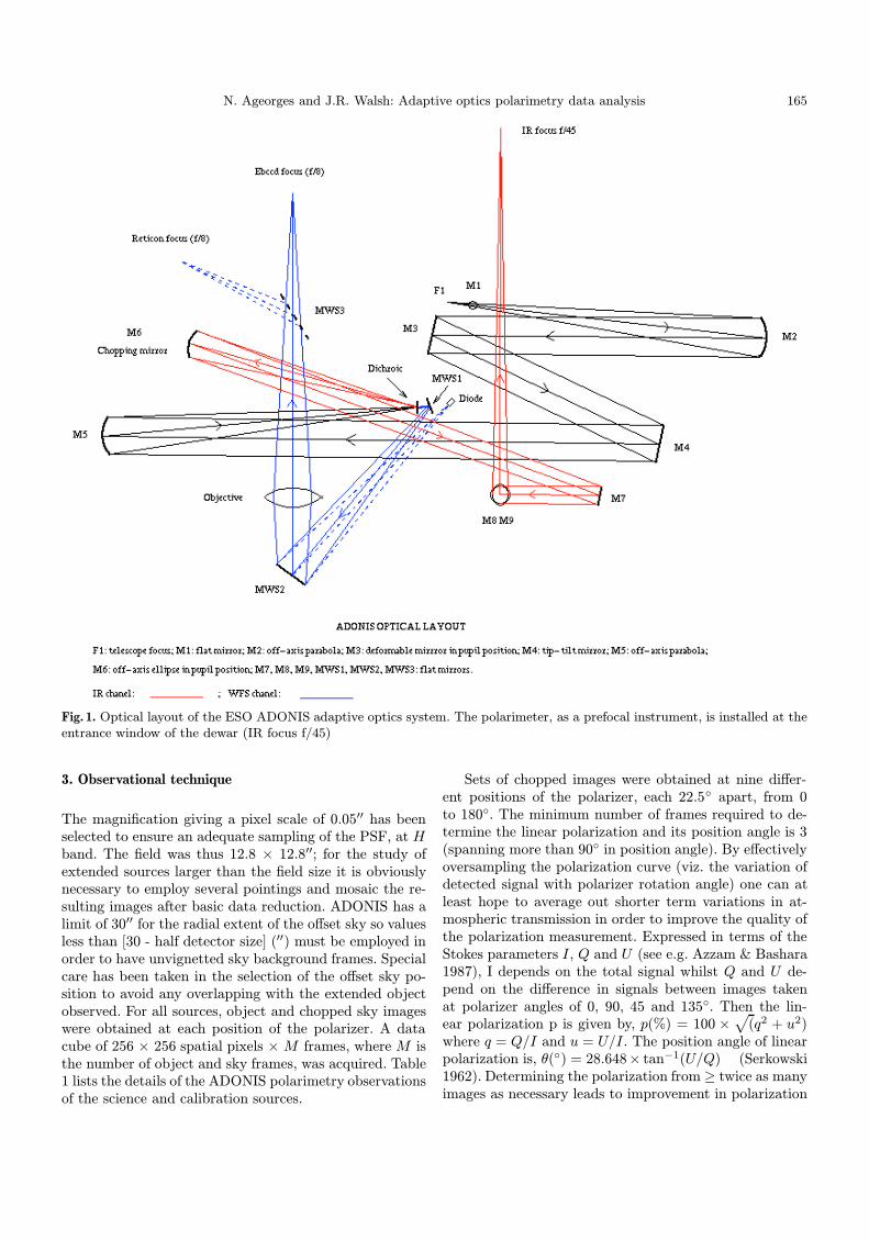
ADONIS is the ADaptive Optics Near Infrared System(see e.g. Beuzit & Hubin 1993 or Beuzit et al. 1997)supported by ESO for common users since December1994 at the F/8.1 Cassegrain focus of the La Silla 3.6 mtelescope. Figure 1 shows the optical layout of theADONIS adaptive optics (AO) system. A tip-tiltand a 64 element deformable mirror corrects thedistortions of the image in real time and a Shack-Hartmann wavefront sensor (WFS) provides thedifference signal for the deformable mirror using abright reference star close to the object. The detec-tor for the Shack Hartmann sensor can be chosen aseither an intensified Reticon for bright sources (mv

< 8 mag) or an electron bombarded CCD for faintersources (8 < mv < 13 mag, 25 to 200 Hz sampling). Bothdetectors are sensitive in the visible wavelength region.An off-axis tiltable mirror allows the sky background, ina field of radius ≤30′′, to be chopped with the on-sourceimage. The output F/45 focus delivers the image to anear-IR detector - either a Rockwell 2562 HgCdTe array(SHARP II for 1−2.5 µm, Hofmann et al. 1995) or a LIRHgCdTe 1282 anti-blooming CCD (COMIC for 1− 5 µm,Marco et al. 1996).

2.2. The camera

The SHARP II camera was selected for the near-IR polari-metric observations. This camera has a fast shutter at theinternal cold Lyot stop, allowing integration times as shortas 20 msec. The present observations were made with thestandard J , H, K filter set and a narrow band 2.15 µmcontinuum filter, with a width of 0.017 µm, and denotedhereafter Kc.

2.3. The polarizer

The polarizer, from Graseby Inc., is a wire grid of 0.25 µmperiod, on a CaF2 subtrate. It is especially designed towork in the spectral range 1 to 9 µm and has a transmis-sion of 83% perpendicular to the wire grid at 1.5 µm. Itis remotely rotated by the ADOCAM control system toany desired absolute position angle within tolerances of0.1◦. This polarizer, as a pre-focal instrument, is insertedinto the beam in front of the camera; and is not cooled.However since the polarizer is not oriented perfectly per-pendicular to the optical axis there is a small image motionon the detector when rotating the polarizer (see Sect. 4.4and Fig. 5).

N. Ageorges and J.R. Walsh: Adaptive optics polarimetry data analysis 165

Fig. 1. Optical layout of the ESO ADONIS adaptive optics system. The polarimeter, as a prefocal instrument, is installed at theentrance window of the dewar (IR focus f/45)

3. Observational technique

The magnification giving a pixel scale of 0.05′′ has beenselected to ensure an adequate sampling of the PSF, at Hband. The field was thus 12.8 × 12.8′′; for the study ofextended sources larger than the field size it is obviouslynecessary to employ several pointings and mosaic the re-sulting images after basic data reduction. ADONIS has alimit of 30′′ for the radial extent of the offset sky so valuesless than [30 - half detector size] (′′) must be employed inorder to have unvignetted sky background frames. Specialcare has been taken in the selection of the offset sky po-sition to avoid any overlapping with the extended objectobserved. For all sources, object and chopped sky imageswere obtained at each position of the polarizer. A datacube of 256 × 256 spatial pixels × M frames, where M isthe number of object and sky frames, was acquired. Table1 lists the details of the ADONIS polarimetry observationsof the science and calibration sources.

Sets of chopped images were obtained at nine differ-ent positions of the polarizer, each 22.5◦ apart, from 0to 180◦. The minimum number of frames required to de-termine the linear polarization and its position angle is 3(spanning more than 90◦ in position angle). By effectivelyoversampling the polarization curve (viz. the variation ofdetected signal with polarizer rotation angle) one can atleast hope to average out shorter term variations in at-mospheric transmission in order to improve the quality ofthe polarization measurement. Expressed in terms of theStokes parameters I, Q and U (see e.g. Azzam & Bashara1987), I depends on the total signal whilst Q and U de-pend on the difference in signals between images takenat polarizer angles of 0, 90, 45 and 135◦. Then the lin-ear polarization p is given by, p(%) = 100 ×

√(q2 + u2)

where q = Q/I and u = U/I. The position angle of linearpolarization is, θ(◦) = 28.648× tan−1(U/Q) (Serkowski1962). Determining the polarization from ≥ twice as manyimages as necessary leads to improvement in polarization


accuracy provided that any photometric variations are ontimescales different from the exposure time of individualimages at each polarizer angle. The worst case scenario iswhen photometric variations occur on a timescale similarto the exposure times, so that the measured difference sig-nals vary wildy - the polarization determined by fitting acosine curve then approaches zero. The chosen exposuretimes per polarizer angle were in the range 1 to 50 s de-pending on the source brightness (see Table 1). Observinga polarized source with the polarizer at 0 and 180◦ polar-izer positions should give the same detected counts and istherefore a direct way to monitor the photometric vari-ations during the observational sequence. Column 8 ofTable 1 lists half the difference (in percentage) betweenintegrated counts in the star profile for the 0 and 180◦

images (i.e. rms on the mean of the 0 and 180◦ signal val-ues). For R Monocerotis, the semi-stellar peak of the re-flection nebula NGC 2261, the aperture covers the centralextended source (full extent 8′′), whilst for OH 0739−14,a reflection nebula around an embedded young star, anarea 10′′ in size was used for the statistics.

4. Data reduction

The data reduction applied to AO polarimetry data con-sists of the removal of the detector signature and skysubtraction, which is common to IR imaging in general,followed by registration and derivation of the polarizationparameters.

4.1. Removal of the detector signature

The basic data reduction steps were performed with the“eclipse” package (Devillard 1997). Flat-fields were ac-quired on the twilight sky at the beginning of each nightof observation, in an exactly similar way as for the targets,at nine angles of the polarizer. The integration times were7, 10 and 20 s for the J , H and K bands respectively; noflat field was taken with the Kc filter. The flat field imagesmust first be processed to flag bad pixels, caused by eitherpermanently dead pixels or ones whose sensitivity under-goes large fluctuation during the exposure. Two methodshave been employed depending on the number of framesavailable in a cube: sky variation or median threshold.

The “sky variation” method works on a data cube,with preferably many planes (>∼20) in order to obtain re-liable statistics on the variations. The standard deviation(σ) with frame number is computed for each pixel in theframe. A histogram plot of the standard deviations has aGaussian shape representing the response to the, assumedconstant, sky signal. All pixels whose response is too low(dead) or too high (noisy), compared to a central ±σ/2 in-terval, are rejected. The “median threshold” method canbe applied to a small number of input frames (such as

flat field data) and detects the presence of spikes above orbelow the local mean in each individual image indepen-dently. If the signal is assumed to be smooth enough, badpixels are found by computing the difference between theimage and its median filtered version, and thresholding it.This latter method is not as stringent as using the tempo-ral variation, but is the only possibility when there are aninsufficient number of images to calculate reliable statis-tics. Some bad pixels may however remain in the imagesafter applying the bad pixel correction by either method;however the number is small and they can be manuallyadded to the bad pixel map. Slightly different bad pixelmaps were found for the different positions of the polar-izer; which could be explained by a polarization sensitivityof the pixels (∼1%), since the NICMOS detector sensitiv-ity is slightly polarization dependent, or simply by therandom variation of hot pixels.

Once corrected for the bad pixels, the twilight flatswere normalized, then multiple exposures were averagedfor the same position of the polarizer to derive the flatfield maps. The target data cubes were corrected with thebad pixel map derived using the “sky variation” methodfrom the background sky frames and divided by the flat-field to give flat-fielded, cleaned images, where the skycontribution is still to be subtracted. All these operationswere performed independently for the nine positions of thepolarizer.

4.2. Sky subtraction

The sky background can be bright in the IR and may alsobe polarized so it is criticical in the case of polarimetryto ensure that the uncertainties introduced by sky sub-traction are minimized. Several tests were performed todetermine the impact of the method of sky subtraction,in conjunction with the bad pixel correction, on the data.The first method considers one sky and a bad pixel mapfor each position of the polarizer; the second method a sin-gle averaged sky (all polarizer positions confounded) butindividual bad pixel maps for each position; whilst thethird method uses the same averaged sky and bad pixelmap for all polarizer angles.

All three methods were tested (Ageorges 1999) and theresults demonstrated that the largest modification of pixelvalues, and therefore photometry, comes from the badpixel map used. The third method produced the largestdiscrepancies from the expected cos(2θ) curve, where θ isthe polarizer position angle. The first method is clearlyto be preferred since the effect of any polarization of thesky signal on the target data is correctly removed and anyshort term variation in sky background is subtracted.

It was found, from sky background level in the polar-ization calibrator data, that the sky subtraction has beensuccessful to better than 1% (rms noise of 3.5 ADUs). Forthe 0 and 180◦ data, a further test of the quality of the sky


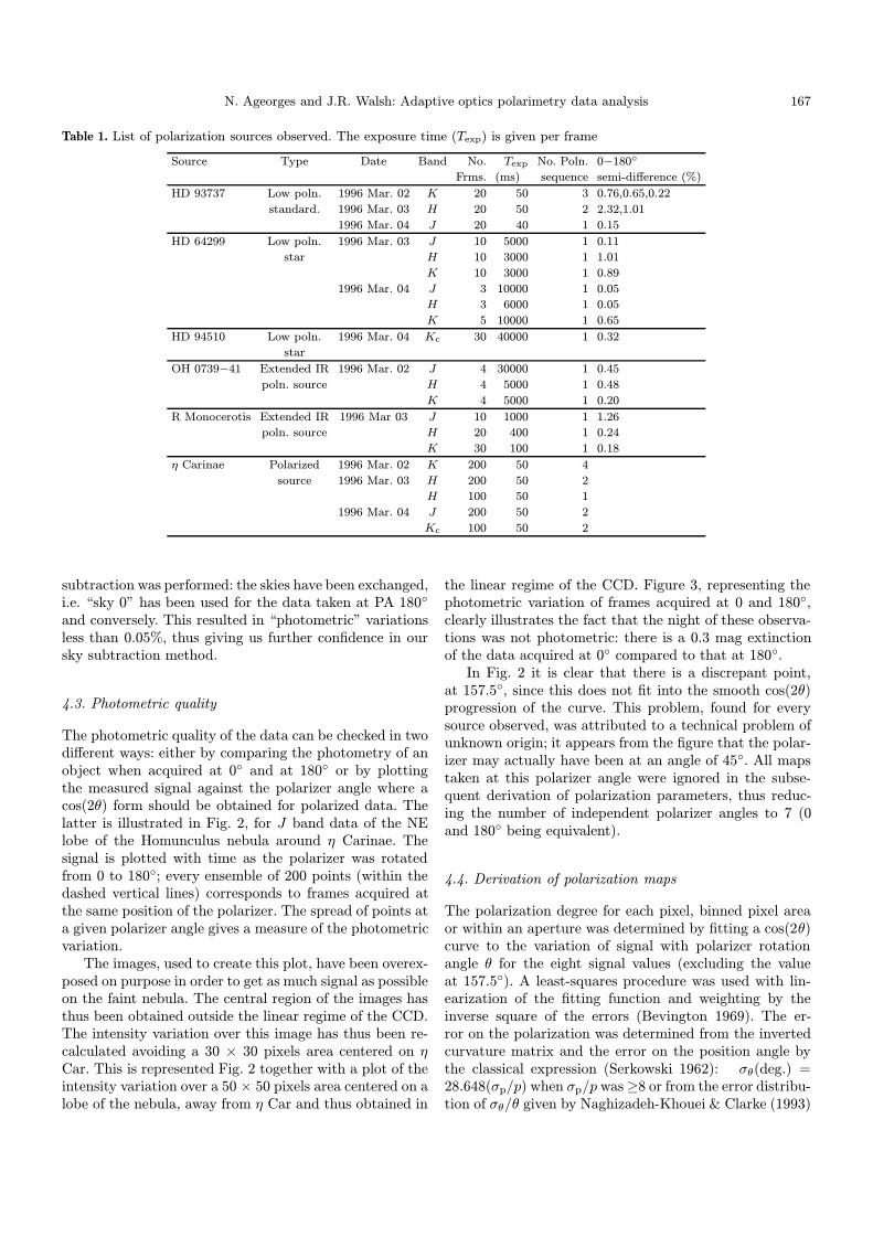
Table 1. List of polarization sources observed. The exposure time (Texp) is given per frame

Source Type Date Band No. Texp No. Poln. 0−180◦

Frms. (ms) sequence semi-difference (%)

HD 93737 Low poln. 1996 Mar. 02 K 20 50 3 0.76,0.65,0.22

standard. 1996 Mar. 03 H 20 50 2 2.32,1.01

1996 Mar. 04 J 20 40 1 0.15

HD 64299 Low poln. 1996 Mar. 03 J 10 5000 1 0.11

star H 10 3000 1 1.01

K 10 3000 1 0.89

1996 Mar. 04 J 3 10000 1 0.05

H 3 6000 1 0.05

K 5 10000 1 0.65

HD 94510 Low poln. 1996 Mar. 04 Kc 30 40000 1 0.32

star

OH 0739−41 Extended IR 1996 Mar. 02 J 4 30000 1 0.45

poln. source H 4 5000 1 0.48

K 4 5000 1 0.20

R Monocerotis Extended IR 1996 Mar 03 J 10 1000 1 1.26

poln. source H 20 400 1 0.24

K 30 100 1 0.18

η Carinae Polarized 1996 Mar. 02 K 200 50 4

source 1996 Mar. 03 H 200 50 2

H 100 50 1

1996 Mar. 04 J 200 50 2

Kc 100 50 2

subtraction was performed: the skies have been exchanged,i.e. “sky 0” has been used for the data taken at PA 180◦

and conversely. This resulted in “photometric” variationsless than 0.05%, thus giving us further confidence in oursky subtraction method.

4.3. Photometric quality

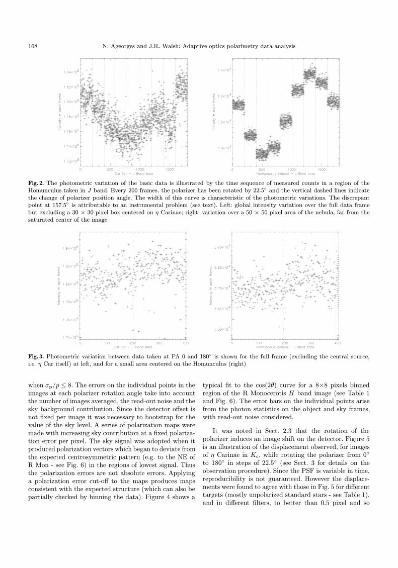
The photometric quality of the data can be checked in twodifferent ways: either by comparing the photometry of anobject when acquired at 0◦ and at 180◦ or by plottingthe measured signal against the polarizer angle where acos(2θ) form should be obtained for polarized data. Thelatter is illustrated in Fig. 2, for J band data of the NElobe of the Homunculus nebula around η Carinae. Thesignal is plotted with time as the polarizer was rotatedfrom 0 to 180◦; every ensemble of 200 points (within thedashed vertical lines) corresponds to frames acquired atthe same position of the polarizer. The spread of points ata given polarizer angle gives a measure of the photometricvariation.

The images, used to create this plot, have been overex-posed on purpose in order to get as much signal as possibleon the faint nebula. The central region of the images hasthus been obtained outside the linear regime of the CCD.The intensity variation over this image has thus been re-calculated avoiding a 30 × 30 pixels area centered on ηCar. This is represented Fig. 2 together with a plot of theintensity variation over a 50 × 50 pixels area centered on alobe of the nebula, away from η Car and thus obtained in

the linear regime of the CCD. Figure 3, representing thephotometric variation of frames acquired at 0 and 180◦,clearly illustrates the fact that the night of these observa-tions was not photometric: there is a 0.3 mag extinctionof the data acquired at 0◦ compared to that at 180◦.

In Fig. 2 it is clear that there is a discrepant point,at 157.5◦, since this does not fit into the smooth cos(2θ)progression of the curve. This problem, found for everysource observed, was attributed to a technical problem ofunknown origin; it appears from the figure that the polar-izer may actually have been at an angle of 45◦. All mapstaken at this polarizer angle were ignored in the subse-quent derivation of polarization parameters, thus reduc-ing the number of independent polarizer angles to 7 (0and 180◦ being equivalent).

4.4. Derivation of polarization maps

The polarization degree for each pixel, binned pixel areaor within an aperture was determined by fitting a cos(2θ)curve to the variation of signal with polarizer rotationangle θ for the eight signal values (excluding the valueat 157.5◦). A least-squares procedure was used with lin-earization of the fitting function and weighting by theinverse square of the errors (Bevington 1969). The er-ror on the polarization was determined from the invertedcurvature matrix and the error on the position angle bythe classical expression (Serkowski 1962): σθ(deg.) =28.648(σp/p) when σp/p was≥8 or from the error distribu-tion of σθ/θ given by Naghizadeh-Khouei & Clarke (1993)


Fig. 2. The photometric variation of the basic data is illustrated by the time sequence of measured counts in a region of theHomunculus taken in J band. Every 200 frames, the polarizer has been rotated by 22.5◦ and the vertical dashed lines indicatethe change of polarizer position angle. The width of this curve is characteristic of the photometric variations. The discrepantpoint at 157.5◦ is attributable to an instrumental problem (see text). Left: global intensity variation over the full data framebut excluding a 30 × 30 pixel box centered on η Carinae; right: variation over a 50 × 50 pixel area of the nebula, far from thesaturated center of the image

Fig. 3. Photometric variation between data taken at PA 0 and 180◦ is shown for the full frame (excluding the central source,i.e. η Car itself) at left, and for a small area centered on the Homunculus (right)

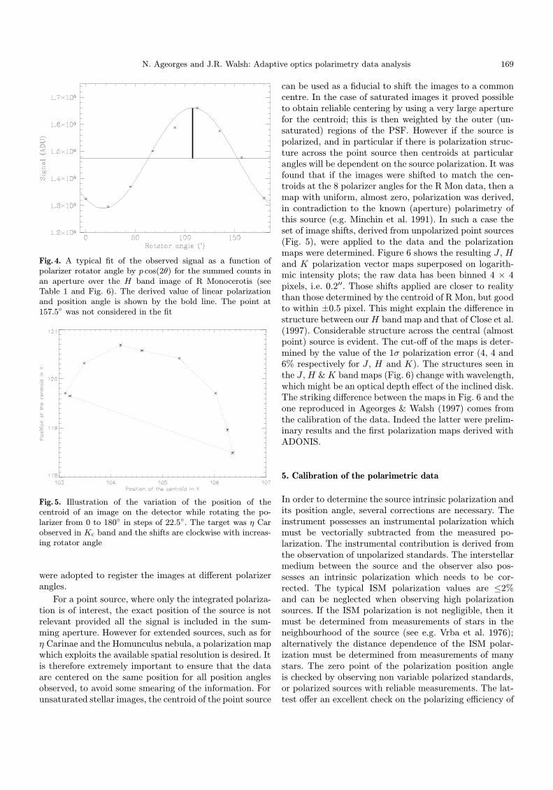
when σp/p ≤ 8. The errors on the individual points in theimages at each polarizer rotation angle take into accountthe number of images averaged, the read-out noise and thesky background contribution. Since the detector offset isnot fixed per image it was necessary to bootstrap for thevalue of the sky level. A series of polarization maps weremade with increasing sky contribution at a fixed polariza-tion error per pixel. The sky signal was adopted when itproduced polarization vectors which began to deviate fromthe expected centrosymmetric pattern (e.g. to the NE ofR Mon - see Fig. 6) in the regions of lowest signal. Thusthe polarization errors are not absolute errors. Applyinga polarization error cut-off to the maps produces mapsconsistent with the expected structure (which can also bepartially checked by binning the data). Figure 4 shows a

typical fit to the cos(2θ) curve for a 8×8 pixels binnedregion of the R Monocerotis H band image (see Table 1and Fig. 6). The error bars on the individual points arisefrom the photon statistics on the object and sky frames,with read-out noise considered.

It was noted in Sect. 2.3 that the rotation of thepolarizer induces an image shift on the detector. Figure 5is an illustration of the displacement observed, for imagesof η Carinae in Kc, while rotating the polarizer from 0◦

to 180◦ in steps of 22.5◦ (see Sect. 3 for details on theobservation procedure). Since the PSF is variable in time,reproducibility is not guaranteed. However the displace-ments were found to agree with those in Fig. 5 for differenttargets (mostly unpolarized standard stars - see Table 1),and in different filters, to better than 0.5 pixel and so


Fig. 4. A typical fit of the observed signal as a function ofpolarizer rotator angle by p cos(2θ) for the summed counts inan aperture over the H band image of R Monocerotis (seeTable 1 and Fig. 6). The derived value of linear polarizationand position angle is shown by the bold line. The point at157.5◦ was not considered in the fit

Fig. 5. Illustration of the variation of the position of thecentroid of an image on the detector while rotating the po-larizer from 0 to 180◦ in steps of 22.5◦. The target was η Carobserved in Kc band and the shifts are clockwise with increas-ing rotator angle

were adopted to register the images at different polarizerangles.

For a point source, where only the integrated polariza-tion is of interest, the exact position of the source is notrelevant provided all the signal is included in the sum-ming aperture. However for extended sources, such as forη Carinae and the Homunculus nebula, a polarization mapwhich exploits the available spatial resolution is desired. Itis therefore extremely important to ensure that the dataare centered on the same position for all position anglesobserved, to avoid some smearing of the information. Forunsaturated stellar images, the centroid of the point source

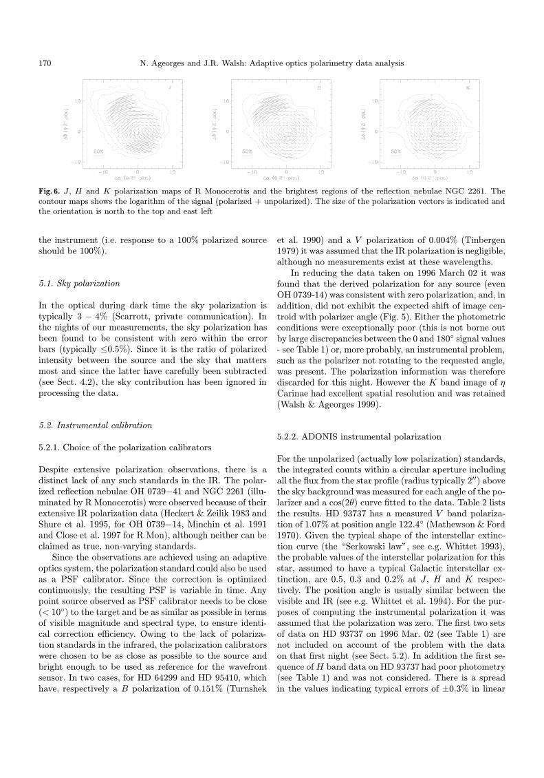
can be used as a fiducial to shift the images to a commoncentre. In the case of saturated images it proved possibleto obtain reliable centering by using a very large aperturefor the centroid; this is then weighted by the outer (un-saturated) regions of the PSF. However if the source ispolarized, and in particular if there is polarization struc-ture across the point source then centroids at particularangles will be dependent on the source polarization. It wasfound that if the images were shifted to match the cen-troids at the 8 polarizer angles for the R Mon data, then amap with uniform, almost zero, polarization was derived,in contradiction to the known (aperture) polarimetry ofthis source (e.g. Minchin et al. 1991). In such a case theset of image shifts, derived from unpolarized point sources(Fig. 5), were applied to the data and the polarizationmaps were determined. Figure 6 shows the resulting J , Hand K polarization vector maps superposed on logarith-mic intensity plots; the raw data has been binned 4 × 4pixels, i.e. 0.2′′. Those shifts applied are closer to realitythan those determined by the centroid of R Mon, but goodto within ±0.5 pixel. This might explain the difference instructure between our H band map and that of Close et al.(1997). Considerable structure across the central (almostpoint) source is evident. The cut-off of the maps is deter-mined by the value of the 1σ polarization error (4, 4 and6% respectively for J , H and K). The structures seen inthe J , H & K band maps (Fig. 6) change with wavelength,which might be an optical depth effect of the inclined disk.The striking difference between the maps in Fig. 6 and theone reproduced in Ageorges & Walsh (1997) comes fromthe calibration of the data. Indeed the latter were prelim-inary results and the first polarization maps derived withADONIS.

5. Calibration of the polarimetric data

In order to determine the source intrinsic polarization andits position angle, several corrections are necessary. Theinstrument possesses an instrumental polarization whichmust be vectorially subtracted from the measured po-larization. The instrumental contribution is derived fromthe observation of unpolarized standards. The interstellarmedium between the source and the observer also pos-sesses an intrinsic polarization which needs to be cor-rected. The typical ISM polarization values are ≤2%and can be neglected when observing high polarizationsources. If the ISM polarization is not negligible, then itmust be determined from measurements of stars in theneighbourhood of the source (see e.g. Vrba et al. 1976);alternatively the distance dependence of the ISM polar-ization must be determined from measurements of manystars. The zero point of the polarization position angleis checked by observing non variable polarized standards,or polarized sources with reliable measurements. The lat-test offer an excellent check on the polarizing efficiency of


Fig. 6. J , H and K polarization maps of R Monocerotis and the brightest regions of the reflection nebulae NGC 2261. Thecontour maps shows the logarithm of the signal (polarized + unpolarized). The size of the polarization vectors is indicated andthe orientation is north to the top and east left

the instrument (i.e. response to a 100% polarized sourceshould be 100%).

5.1. Sky polarization

In the optical during dark time the sky polarization istypically 3 − 4% (Scarrott, private communication). Inthe nights of our measurements, the sky polarization hasbeen found to be consistent with zero within the errorbars (typically ≤0.5%). Since it is the ratio of polarizedintensity between the source and the sky that mattersmost and since the latter have carefully been subtracted(see Sect. 4.2), the sky contribution has been ignored inprocessing the data.

5.2. Instrumental calibration

5.2.1. Choice of the polarization calibrators

Despite extensive polarization observations, there is adistinct lack of any such standards in the IR. The polar-ized reflection nebulae OH 0739−41 and NGC 2261 (illu-minated by R Monocerotis) were observed because of theirextensive IR polarization data (Heckert & Zeilik 1983 andShure et al. 1995, for OH 0739−14, Minchin et al. 1991and Close et al. 1997 for R Mon), although neither can beclaimed as true, non-varying standards.

Since the observations are achieved using an adaptiveoptics system, the polarization standard could also be usedas a PSF calibrator. Since the correction is optimizedcontinuously, the resulting PSF is variable in time. Anypoint source observed as PSF calibrator needs to be close(< 10◦) to the target and be as similar as possible in termsof visible magnitude and spectral type, to ensure identi-cal correction efficiency. Owing to the lack of polariza-tion standards in the infrared, the polarization calibratorswere chosen to be as close as possible to the source andbright enough to be used as reference for the wavefrontsensor. In two cases, for HD 64299 and HD 95410, whichhave, respectively a B polarization of 0.151% (Turnshek

et al. 1990) and a V polarization of 0.004% (Tinbergen1979) it was assumed that the IR polarization is negligible,although no measurements exist at these wavelengths.

In reducing the data taken on 1996 March 02 it wasfound that the derived polarization for any source (evenOH 0739-14) was consistent with zero polarization, and, inaddition, did not exhibit the expected shift of image cen-troid with polarizer angle (Fig. 5). Either the photometricconditions were exceptionally poor (this is not borne outby large discrepancies between the 0 and 180◦ signal values- see Table 1) or, more probably, an instrumental problem,such as the polarizer not rotating to the requested angle,was present. The polarization information was thereforediscarded for this night. However the K band image of ηCarinae had excellent spatial resolution and was retained(Walsh & Ageorges 1999).

5.2.2. ADONIS instrumental polarization

For the unpolarized (actually low polarization) standards,the integrated counts within a circular aperture includingall the flux from the star profile (radius typically 2′′) abovethe sky background was measured for each angle of the po-larizer and a cos(2θ) curve fitted to the data. Table 2 liststhe results. HD 93737 has a measured V band polariza-tion of 1.07% at position angle 122.4◦ (Mathewson & Ford1970). Given the typical shape of the interstellar extinc-tion curve (the “Serkowski law”, see e.g. Whittet 1993),the probable values of the interstellar polarization for thisstar, assumed to have a typical Galactic interstellar ex-tinction, are 0.5, 0.3 and 0.2% at J , H and K respec-tively. The position angle is usually similar between thevisible and IR (see e.g. Whittet et al. 1994). For the pur-poses of computing the instrumental polarization it wasassumed that the polarization was zero. The first two setsof data on HD 93737 on 1996 Mar. 02 (see Table 1) arenot included on account of the problem with the dataon that first night (see Sect. 5.2). In addition the first se-quence of H band data on HD 93737 had poor photometry(see Table 1) and was not considered. There is a spreadin the values indicating typical errors of ±0.3% in linear


Table 2. Polarization of low polarization stars - instrumentalpolarization measurement

Target Date J H K Kc

Linear poln. (%) & PA (◦)

HD 93737 1996 Mar. 02 1.71, 88

1996 Mar. 03 1.59, 89

HD 64299 1996 Mar. 03 1.51, 111 1.99, 86 2.16, 136

1996 Mar. 04 1.67, 97 1.48, 112 1.71, 89

HD 94510 1994 Mar. 04 2.12, 104 2.05, 140

Mean - 1.74, 105 1.69, 96 1.86, 104

Adopted - 1.7, 105 1.7, 90 1.7, 90 2.0, 140

polarization and ±15◦ in position angle. Given the errorsthe J , H and K values are consistent with an instrumentalpolarization of 1.7%. Adopted values are listed in the lastrow of the Table 2. Given that only a single measurementwas performed at Kc, it is probably not significant thatthe instrumental polarization in this band is higher andthat the position angle differs from the K band measure-ment.

Once the instrumental polarization (intensity andangle) is determined this correction can be applied tothe polarization maps point-by-point. Goodrich (1986, inAppendix) describes the application of the instrumentalcorrection.

5.2.3. Position angle calibration

On producing polarization maps for the Homunculusnebula around η Carinae, it was noticed that the polar-ization vectors did not point back to the position of ηCarinae. There is no reason for such a behaviour sinceit is known to be a reflection nebula. If the illuminationwere by an extended source then the offset should notbe one of simple rotation. A novel method was usedto determine the single offset required to align all thepolarization vectors in a centrosymmetric pattern aroundthe position of η Carinae. A least squares problem wassolved to minimize the impact parameter at the positionof η Carinae produced by the perpendiculars to all thepolarization vectors in the Homunculus by applicationof a single rotation. A consistent value of 18 ± 1◦ wasfound for the J , H and K images. In order to verifythat this was not an artifact of the η Carinae nebulaand the fact that the central point source was saturated,the 18◦ correction was applied to the polarization mapsof NGC 2261. It was found that the vectors in the highpolarization spur to the NE were well aligned with thedirection expected for illumination by the peak of R Mon.Thus the calibration of the absolute position angle canbe made without reference to a polarized standard.

Table 3. JHK Polarization of R Monocerotis in an 8′′ aperture

Data source Polarization (%) & PA (◦)

J H K

This work (PA uncorrected) 10.6, 77 11.1, 74 8.1, 77

Minchin et al. (1991) 11.1, 100 8.5, 103 5.6, 102

6. Results on restoration of polarization images

In order to measure polarization structure in the vicin-ity of a bright point source, it is necessary to deconvolvethe point source response from the data frames taken ateach position angle of the polarizer and then to form thepolarization maps from the deconvolved images. The aimhere is to detect polarization structure within an offset dis-tance of a few times the diffraction limit from the pointsource. Several different approaches to restoration havebeen attempted in order to obtain detailed informationon the fine structure of the Homunculus nebula close tothe central source η Carinae. This was motivated by theneed to detect and measure the polarization of the threeknots found in the 0.4′′ vicinity of η Car by speckle imag-ing in the optical (Weigelt & Ebersberger 1986 and Falckeet al. 1996). The polarization data for η Car will be usedto exemplify these experiments; the scientific conclusionswill be reported in Walsh & Ageorges (1999). A prelim-inary discussion of restoration of these images, withoutconsidering the polarization, has been given by Ageorges& Walsh (1998).

6.1. Image restoration trial

Two deconvolution techniques have been applied to thedata: Richardson-Lucy (R-L) iterative deconvolution(Lucy 1974; Richardson 1972) and blind deconvolution(“IDAC”, Jefferies & Christou 1993; Christou et al. 1997).The major difference between these methods is related tothe treatment of the point spread function (PSF). Withthe Richardson-Lucy method, a PSF is required a priorito deconvolve the data, while for blind deconvolution,the PSF is determined from variations in the targetobject data. The blind deconvolution method uses aninitial estimate, which can be a Gaussian for example.Since the adaptive optics PSF changes with time andis not spatially invariant (see e.g. Christou et al. 1998),blind deconvolution should be better suited than theRichardson-Lucy method, which assumes a PSF constantin time. The exact spatial variation of the AO PSF isnot known. However in the present case, this is a minorproblem since the source itself (η Car) has been used aswavefront sensor reference star. Moreover with the pixelscale chosen, all the valuable information in the shortband data is enclosed in the isoplanatic angle; the spatialvariation of the PSF is thus negligible over the area of


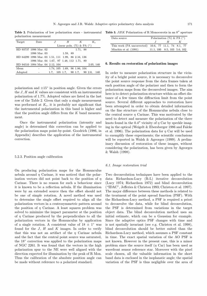
Fig. 7. Comparison of the results of two deconvolution techniques for Kc data of η Carinae and the Homunculus nebula. On thetop row are shown data from the second polarizer sequence, at 0 (left) and 180◦ (right), both deconvolved with “plucy” andconvolved with a Gaussian of 3 pixels FWHM. The bottom left image is identical to the top left one but the data restored isfrom the first polarizer sequence (0◦ image). The result of blind deconvolution is presented in the bottom right hand image forthe first data set - K1

c - at 0◦ polarizer angle

the η Carinae images, which is not the case for the timevariation.

A comparison of the Richardson-Lucy method andIDAC - “Iterative Deconvolution Algorithm in C”, i.e. theblind deconvolution algorithm used, was made using theKc data on η Car (Table 2). The aim was to test the re-ality of structures revealed in the near environment of thecentral star of this reflection nebula. For the R-L restora-tion, the Lucy-Hook algorithm (Hook & Lucy 1994), in itssoftware implementation under IRAF (“plucy”), was em-ployed. The principle is the same as for the Richardson-Lucy method, except that it restores in two channels, onefor the point source and the other for the background (con-sidered smooth at some spatial scale). The estimated posi-tion of the point source is provided and the initial guess forthe background is flat. Kc data taken at polarizer anglesof 0 and 180◦ were restored (called Kc0 and Kc180). Forthe Kc0 image, blind deconvolution was also performed.It should be noted that although the polarizer angles are

effectively identical, the Strehl ratio is not identical be-tween the two data sets (K1

c & K2c ) and is higher for K1

c

(27.9% against 22.1%). Although this could be consideredan advantage, it has a drawback since the four bumpsaround the PSF (see Fig. 8 for the appearance of the PSF)are more pronounced. These bumps (“waffle pattern”) cor-respond to a null mode of the wavefront sensor as a resultof an inadequacy in the control loop. The problem of thefour bumps distributed symetrically around the source isthat although they are in the PSF they do not vary; theyare fixed in time and position and therefore not removedfrom the image as part of the PSF. There is however a wayto overcome this problem, and that is by forcing them tobe in the PSF.

Figure 7 presents the deconvolution results obtainedwith both methods on the two separate data sets (Table 1)and Fig. 8 shows the PSF derived from blind deconvolu-tion. The “plucy” deconvolved data have been restoredto convergence and then convolved with a Gaussian of


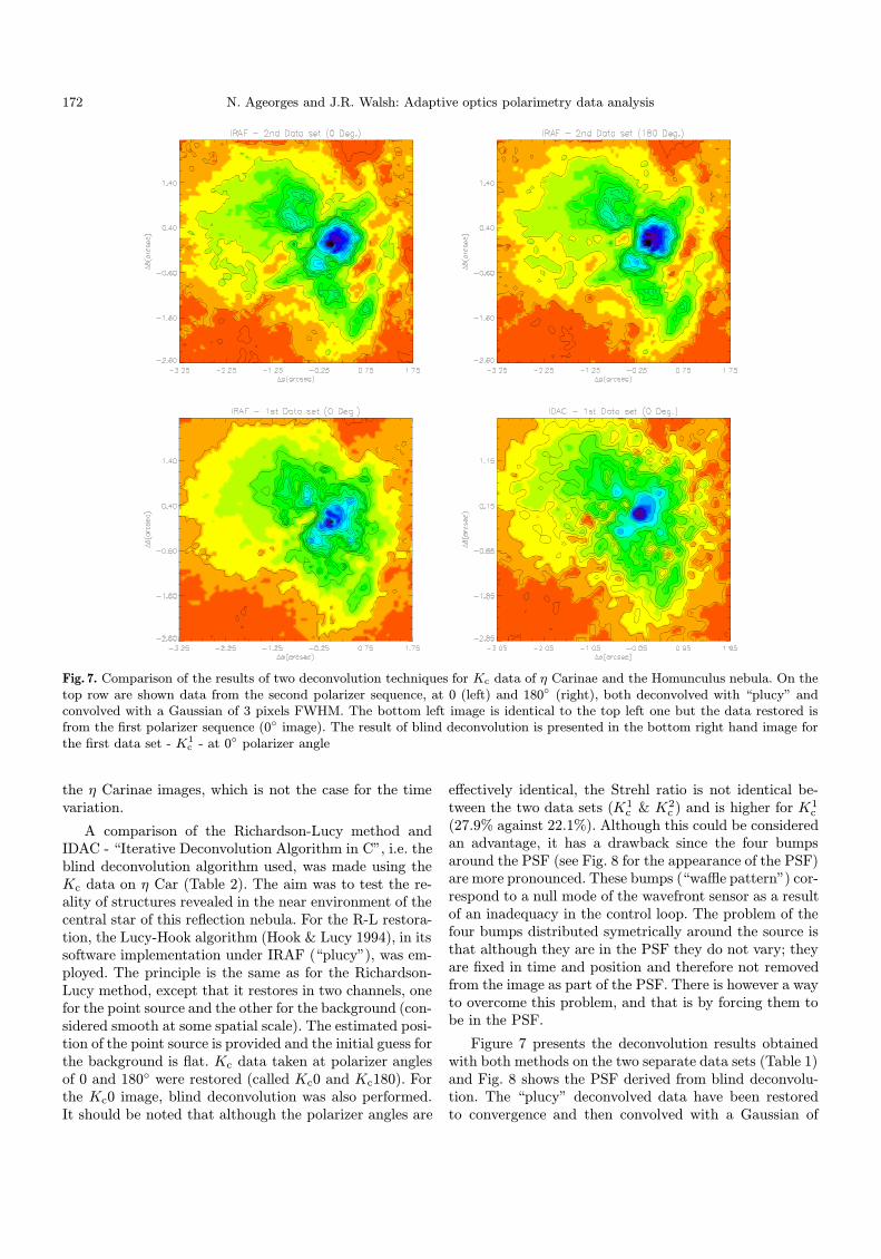
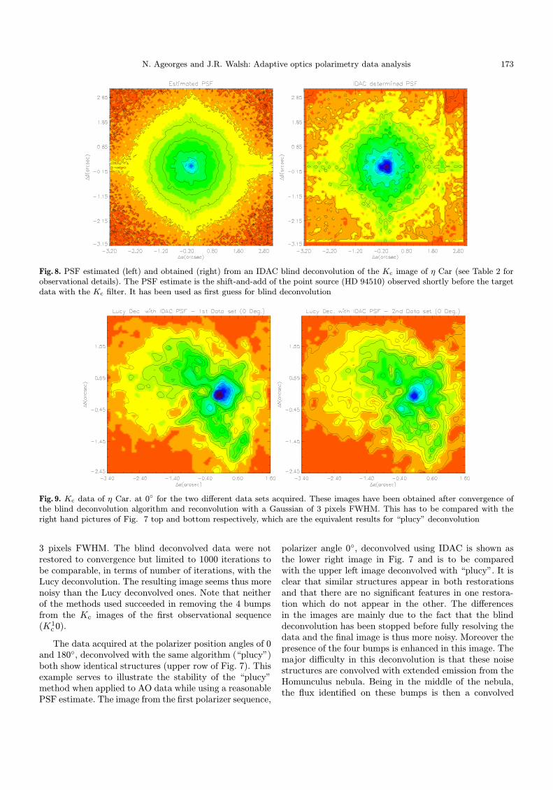
Fig. 8. PSF estimated (left) and obtained (right) from an IDAC blind deconvolution of the Kc image of η Car (see Table 2 forobservational details). The PSF estimate is the shift-and-add of the point source (HD 94510) observed shortly before the targetdata with the Kc filter. It has been used as first guess for blind deconvolution

Fig. 9. Kc data of η Car. at 0◦ for the two different data sets acquired. These images have been obtained after convergence ofthe blind deconvolution algorithm and reconvolution with a Gaussian of 3 pixels FWHM. This has to be compared with theright hand pictures of Fig. 7 top and bottom respectively, which are the equivalent results for “plucy” deconvolution

3 pixels FWHM. The blind deconvolved data were notrestored to convergence but limited to 1000 iterations tobe comparable, in terms of number of iterations, with theLucy deconvolution. The resulting image seems thus morenoisy than the Lucy deconvolved ones. Note that neitherof the methods used succeeded in removing the 4 bumpsfrom the Kc images of the first observational sequence(K1

c 0).

The data acquired at the polarizer position angles of 0and 180◦, deconvolved with the same algorithm (“plucy”)both show identical structures (upper row of Fig. 7). Thisexample serves to illustrate the stability of the “plucy”method when applied to AO data while using a reasonablePSF estimate. The image from the first polarizer sequence,

polarizer angle 0◦, deconvolved using IDAC is shown asthe lower right image in Fig. 7 and is to be comparedwith the upper left image deconvolved with “plucy”. It isclear that similar structures appear in both restorationsand that there are no significant features in one restora-tion which do not appear in the other. The differencesin the images are mainly due to the fact that the blinddeconvolution has been stopped before fully resolving thedata and the final image is thus more noisy. Moreover thepresence of the four bumps is enhanced in this image. Themajor difficulty in this deconvolution is that these noisestructures are convolved with extended emission from theHomunculus nebula. Being in the middle of the nebula,the flux identified on these bumps is then a convolved


product of the waffle pattern and the extended structureof the nebula. It is thus very difficult for the programto isolate these four “point sources” and recover properlythe true shape of the nebula at these positions. In orderto fully compare the different deconvolution techniques,blind deconvolution has been pushed to convergence forKc0 (data set 1 & 2). The results (Fig. 9) are to be com-pared with the right hand side of Fig. 7. The structuresclose to η Car emphasized by the two deconvolution pro-cesses, excluding the four bumps, confer a degree of con-fidence in the scientific results which will be presented inWalsh & Ageorges (1999).

6.2. Polarimetry restoration trial

In the case of polarimetric data, the deconvolutionproblem is more severe since the photometry must bepreserved in the restored images in order to derive apolarization map. The Richardson-Lucy algorithm issuperior to blind deconvolution in that it should preserveflux. Experiments were performed on the Kc η Car dataset, restoring each of the nine polarizer images with thePSF derived from the unpolarized standard at the samepolarizer angle. The results were poor even when therestored image was convolved with a Gaussian of 3 pixelsFWHM. They illustrate the effect of the variable PSF andthus the difficulty to recover polarization data at highangular resolution so close to the star. Huge fluctuationsin the value of the polarization were seen in the vicinityof η Car. The differing PSF of the unpolarized star andof η Car (the AO correction was much better for the ηCar images than for the standard star) produced restoredimages with large differences in flux at a given pixel inthe different polarization images. At present there is noknown method to recover the true PSF from the dataand conserve the flux through restoration. A possible(although computer intensive) solution is to determinethe PSF from blind deconvolution and use the resultfor the PSF in another algorithm known to preserve theflux. This has been performed here: the PSF determinedby blind deconvolution has been used both with theRichardson-Lucy and Lucy-Hook algorithms. Since theIDAC blind deconvolution algorithm normalised the inputimage at the beginning of the iterations, the final imagewas rescaled back to the original total count to allowerror estimation of the polarization image. Polarizationmaps for the three methods (“IDAC” alone and combinedwith R-L and “plucy” methods) have been created andcompared after reconvolution with a 3 pixel Gaussian.

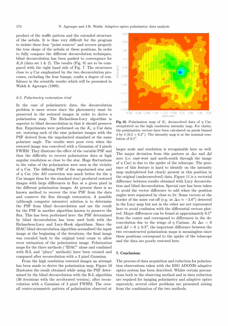
From the high resolution restored images an attempthas been made to derive the polarization map. Figure 10illustrates the result obtained while using the PSF deter-mined by the blind deconvolution with the R-L algorithm(30 iterations with the accelerated version), after recon-volution with a Gaussian of 3 pixel FWHM. The over-all centro-symmetric pattern of polarization observed at

Fig. 10. Polarization map of Kc deconvolved data of η Car.overplotted on the high resolution intensity map. For clarity,the polarization vectors have been calculated on pixels binned4 by 4 (0.2 × 0.2′′). The intensity map is at the nominal reso-lution of 0.1′′

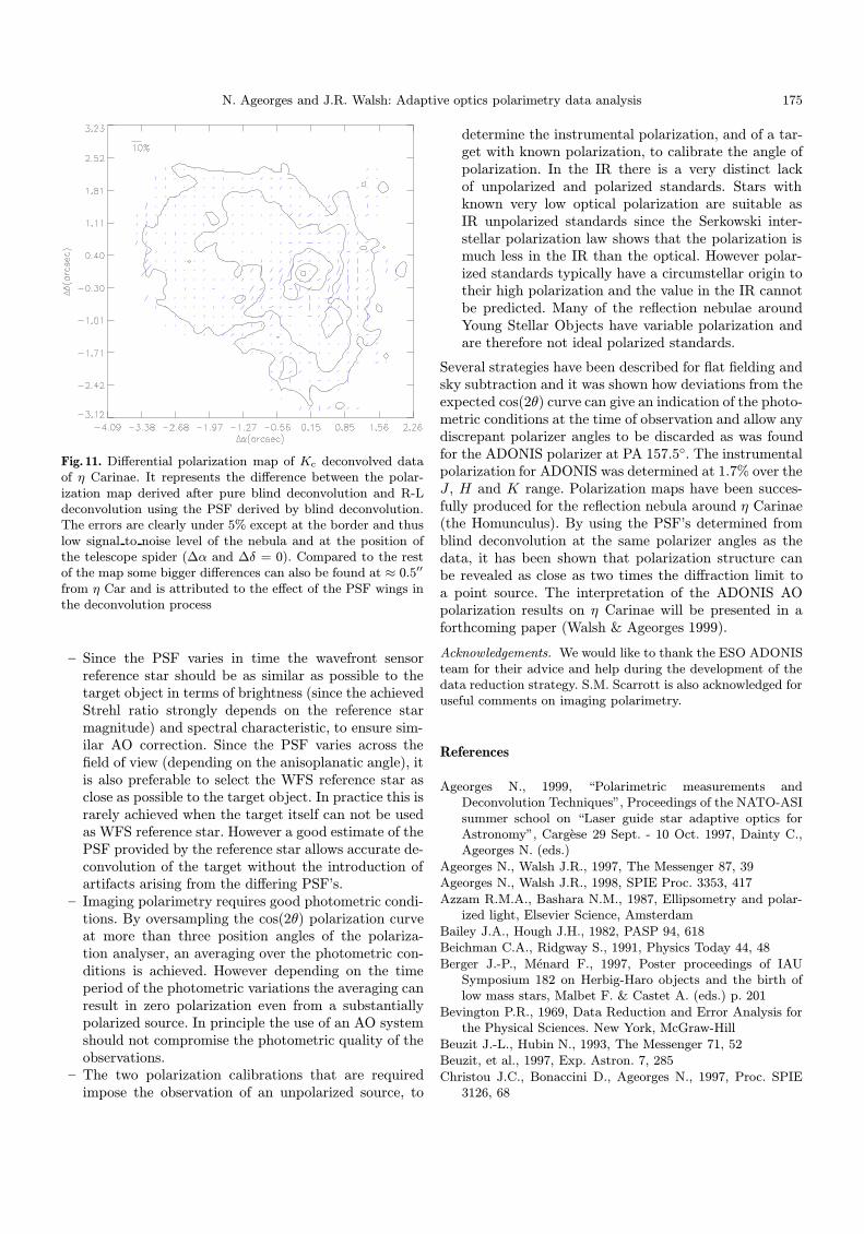
larger scale and resolution is recognisable here as well.The major deviation from this pattern at ∆α and ∆δzero (i.e. east-west and north-south through the imageof η Car) is due to the spider of the telescope. The pres-ence of this feature is hard to identify on the intensitymap underplotted but clearly present at this position inthe original (undeconvolved) data. Figure 11 is a vectorialdifference between results obtained with Lucy deconvolu-tion and blind deconvolution. Special care has been takento avoid the vector difference to add when the positionangles were separated by close to 2π. Some vectors at theborder of the noise cut-off (e.g. at ∆α ≈ −3.0′′) detectedin the Lucy map but not in the other are not representedhere to avoid confusion with the differential vectors plot-ted. Major differences can be found at approximately 0.5′′

from the center and correspond to differences in the de-convolution due to the wings of η Carinae. At ∆α = 0and ∆δ = 0 ± 0.3′′, the important difference between thetwo reconstructed polarization maps is meaningless sincethese positions correspond to the spider of the telescopeand the data are poorly restored here.

7. Conclusions

The process of data acquisition and reduction for polariza-tion observations taken with the ESO ADONIS adaptiveoptics system has been described. Whilst certain precau-tions both in the observing method and in data reductionare required for imaging polarimetry and adaptive opticsseperately, several other problems are presented arisingfrom the combination of the two methods.


Fig. 11. Differential polarization map of Kc deconvolved dataof η Carinae. It represents the difference between the polar-ization map derived after pure blind deconvolution and R-Ldeconvolution using the PSF derived by blind deconvolution.The errors are clearly under 5% except at the border and thuslow signal to noise level of the nebula and at the position ofthe telescope spider (∆α and ∆δ = 0). Compared to the restof the map some bigger differences can also be found at ≈ 0.5′′

from η Car and is attributed to the effect of the PSF wings inthe deconvolution process

– Since the PSF varies in time the wavefront sensorreference star should be as similar as possible to thetarget object in terms of brightness (since the achievedStrehl ratio strongly depends on the reference starmagnitude) and spectral characteristic, to ensure sim-ilar AO correction. Since the PSF varies across thefield of view (depending on the anisoplanatic angle), itis also preferable to select the WFS reference star asclose as possible to the target object. In practice this israrely achieved when the target itself can not be usedas WFS reference star. However a good estimate of thePSF provided by the reference star allows accurate de-convolution of the target without the introduction ofartifacts arising from the differing PSF’s.

– Imaging polarimetry requires good photometric condi-tions. By oversampling the cos(2θ) polarization curveat more than three position angles of the polariza-tion analyser, an averaging over the photometric con-ditions is achieved. However depending on the timeperiod of the photometric variations the averaging canresult in zero polarization even from a substantiallypolarized source. In principle the use of an AO systemshould not compromise the photometric quality of theobservations.

– The two polarization calibrations that are requiredimpose the observation of an unpolarized source, to

determine the instrumental polarization, and of a tar-get with known polarization, to calibrate the angle ofpolarization. In the IR there is a very distinct lackof unpolarized and polarized standards. Stars withknown very low optical polarization are suitable asIR unpolarized standards since the Serkowski inter-stellar polarization law shows that the polarization ismuch less in the IR than the optical. However polar-ized standards typically have a circumstellar origin totheir high polarization and the value in the IR cannotbe predicted. Many of the reflection nebulae aroundYoung Stellar Objects have variable polarization andare therefore not ideal polarized standards.

Several strategies have been described for flat fielding andsky subtraction and it was shown how deviations from theexpected cos(2θ) curve can give an indication of the photo-metric conditions at the time of observation and allow anydiscrepant polarizer angles to be discarded as was foundfor the ADONIS polarizer at PA 157.5◦. The instrumentalpolarization for ADONIS was determined at 1.7% over theJ , H and K range. Polarization maps have been succes-fully produced for the reflection nebula around η Carinae(the Homunculus). By using the PSF’s determined fromblind deconvolution at the same polarizer angles as thedata, it has been shown that polarization structure canbe revealed as close as two times the diffraction limit toa point source. The interpretation of the ADONIS AOpolarization results on η Carinae will be presented in aforthcoming paper (Walsh & Ageorges 1999).

Acknowledgements. We would like to thank the ESO ADONISteam for their advice and help during the development of thedata reduction strategy. S.M. Scarrott is also acknowledged foruseful comments on imaging polarimetry.

References

Ageorges N., 1999, “Polarimetric measurements andDeconvolution Techniques”, Proceedings of the NATO-ASIsummer school on “Laser guide star adaptive optics forAstronomy”, Cargese 29 Sept. - 10 Oct. 1997, Dainty C.,Ageorges N. (eds.)

Ageorges N., Walsh J.R., 1997, The Messenger 87, 39Ageorges N., Walsh J.R., 1998, SPIE Proc. 3353, 417

Azzam R.M.A., Bashara N.M., 1987, Ellipsometry and polar-ized light, Elsevier Science, Amsterdam

Bailey J.A., Hough J.H., 1982, PASP 94, 618Beichman C.A., Ridgway S., 1991, Physics Today 44, 48

Berger J.-P., Menard F., 1997, Poster proceedings of IAUSymposium 182 on Herbig-Haro objects and the birth oflow mass stars, Malbet F. & Castet A. (eds.) p. 201

Bevington P.R., 1969, Data Reduction and Error Analysis forthe Physical Sciences. New York, McGraw-Hill

Beuzit J.-L., Hubin N., 1993, The Messenger 71, 52Beuzit, et al., 1997, Exp. Astron. 7, 285

Christou J.C., Bonaccini D., Ageorges N., 1997, Proc. SPIE3126, 68


Christou J.C., Marchis F., Ageorges N., Bonaccini D., RigautF., 1998, SPIE Proc. 3353, 984

Close L.M., et al., 1997, ApJ 489, 210Code A.D., Whitney B.A., 1995, ApJ 441, 400Davis L. Jr., Greenstein J.L., 1951, ApJ 114, 206Devillard N., 1997, The Messenger 87, 19Draine B.T., Lee H.M., 1984, ApJ 285, 89Falcke H., Davidson K., Hofmann K.-H., Weigelt G., 1996,

A&A 306, L17Fischer O., Henning Th., Yorke H.W., 1994, A&A 284, 187Goodrich R.W., 1986, ApJ 311, 882Heckert P.A., Zeilik M., 1983, MNRAS 202, 531Hodapp K.W., 1984, A&A 141, 255Hofmann R., Brandl B., Eckart A., Eisenhauer F., Tacconi-

Garman L., 1995, Proc. SPIE 2475, 192Hook R.N., Lucy L.B., 1994, Image restorations of high photo-

metric quality. II. Examples. In Hanisch R.J. & White R.L.(eds.) Space Telescope Science Institute, The restoration ofHST images and spectra II, p. 86

Jefferies S.M., Christou J.C., 1993, ApJ 415, 862Jones T.J., 1997, AJ 114, 1393Lloyd-Hart M., et al., 1998, ApJ 493, 950Lucy L., 1974, AJ 79, 745Marco O., Lacombe F., Bonaccini D., 1996, ESO Messenger,

No. 85, 39

Mathewson D.S., Ford V.L., 1970, Mem. RAS 74, 139Mathis J.S., 1990, ARA&A 28, 37Minchin N.R., et al., 1991, MNRAS 249, 707Naghizadeh-Khouei J., Clarke D., 1993, A&A 274, 968Piirola V., Scaltriti F., Coyne G.V., 1992, Nat 359, No. 6394,

399Richardson W.H., 1972, J. Opt. Soc. Am. 62, 55Rigaut F., et al., 1998, PASP 110, 152Sahai R., et al., 1997, ApJ 492, L163Serkowski K., 1962, Kopal Z. (ed.), Adv. in A&A 1, 289Sitko M.L., Yudong Z., 1991, ApJ 369, 106Shure M., Sellgren K., Jones T.J., Klebe D., 1995, AJ 109, 721Tinbergen J., 1979, A&ASS 35, 325Turnshek D.A., et al., 1990, AJ 99, 1243Vrba F.J., Strom S.E., Strom K.M., 1976, AJ 81, 958Walsh J.R., Ageorges N., 1999, A&A (in preparation)Warren-Smith R.F., 1983, MNRAS 205, 337Weigelt G., Ebersberger J., 1986, A&A 163, L5White R.L., Schiffer F.H., Mathis J.S., 1980, ApJ 241, 208Whitney B.A., Hartmann L., 1992, ApJ 395, 529Whittet D.C.B., 1993, Dust in the Galactic Environment,

Bristol, Inst. of Phys.Whittet D.C.B., et al., 1994, MNRAS 268, 1Witt A.N., 1977, ApJS 35, 1

Acquisition and analysis of adaptive optics imaging - CiteSeer

Documents

Transcript of Acquisition and analysis of adaptive optics imaging - CiteSeer