A methodology to constrain the parameters of a hydrogeological discrete fracture network model for...

$: A methodology to constrain the parameters of a hydrogeological discrete fracture network model for sparsely fractured crystalline rock, exemplified by data from the proposed high-level$
A methodology to constrain the parameters of a hydrogeologicaldiscrete fracture network model for sparsely fractured crystallinerock, exemplified by data from the proposed high-level nuclearwaste repository site at Forsmark, Sweden

Sven Follin & Lee Hartley & Ingvar Rhén &

Peter Jackson & Steven Joyce & David Roberts &

Ben Swift

Abstract The large-scale geological structure of thecrystalline rock at the proposed high-level nuclear wasterepository site at Forsmark, Sweden, has been classified interms of deformation zones of elevated fracture frequency.The rock between deformation zones was divided intofracture domains according to fracture frequency. Amethodology to constrain the geometric and hydraulicparameters that define a discrete fracture network (DFN)

model for each fracture domain is presented. Themethodology is based on flow logging and down-holeimaging in cored boreholes in combination with DFNrealizations, fracture connectivity analysis and pumpingtest simulations. The simulations suggest that a goodmatch could be obtained for a power law size distributionwhere the value of the location parameter equals theborehole radius but with different values for the shapeparameter, depending on fracture domain and fracture set.Fractures around 10–100m in size are the ones thattypically form the connected network, giving inflows inthe simulations. The report also addresses the issue of up-scaling of DFN properties to equivalent continuous porousmedium (ECPM) bulk flow properties. Comparisons withdouble-packer injection tests provide confidence that thederived DFN formulation of detailed flows within indi-vidual fractures is also suited to simulating mean bulkflow properties and their spatial variability.

Keywords Crystalline rock . Discrete fracture networkmodeling . Nuclear waste . Sweden . Forsmark

Background

Since the 1980s, a repository for the disposal of highlyradioactive, spent nuclear fuel in Sweden has beenenvisaged by Svensk Kärnbränslehantering AB (SKB)in crystalline bedrock at a depth of about 500 m in theFennoscandian Shield (Fig. 1). Between 2002 and2008, site investigations with characterizations ofrelevant rock properties were carried out at two siteson the southeastern coast of Sweden, at Forsmark andLaxemar (Fig. 1a). In parallel, a site investigation withcharacterization has also been completed at a site onthe southwestern coast of Finland, at Olkiluoto, as partof the Finnish program (Fig. 1). Selroos and Follin(2013) provide an overview of the Swedish programand method for geological disposal of spent nuclearfuel in crystalline bedrock.

Received: 20 November 2012 /Accepted: 7 November 2013Published online: 11 December 2013

* Springer-Verlag Berlin Heidelberg 2013

This article belongs to a series describing site-descriptive modeling ofbedrock hydrogeology for the proposed high-level nuclear wasterepository site at Forsmark, Sweden

S. Follin ())SF GeoLogic AB, Box 1139, SE 183 11 Täby, Swedene-mail: [email protected].: +46-70-5408284

L. Hartley : P. Jackson : S. Joyce :B. SwiftAMEC, Building 150, Harwell Oxford, Didcot, Oxfordshire OX110QB( UK

L. Hartleye-mail: [email protected]

P. Jacksone-mail: [email protected]

S. Joycee-mail: [email protected]

B. Swifte-mail: [email protected]

I. RhénSWECO Environment, Box 2203, SE 101 24 Gothenburg, Swedene-mail: [email protected]

D. RobertsNuclear Decommissioning Authority, Harwell, Didcot, OxfordshireOX11 0RA( UKe-mail: [email protected]

Hydrogeology Journal (2014) 22: 313–331DOI 10.1007/s10040-013-1080-2

One important part of these investigations is to developan integrated site description based on site-specific dataand its regional setting, covering the current state andproperties of the deep rock, the surface system and humanland use, as well as the processes affecting their long-termdevelopment (OECD-NEA 1993; Bath and Lalieux 1999;IAEA 1999; SKB 2001; Andersson et al. 2007; Ström etal. 2008). In brief, the integrated site descriptionsdeveloped in Sweden and Finland (SKB 2008, 2009;Posiva 2009) are basically needed to: (1) develop andpresent the geoscientific and ecological understanding ofthe site; (2) underpin a safety assessment describingdifferent scenarios and consequences if radionuclides arereleased from the repository; (3) establish a baseline fordetecting short- and long-term effects of the repository; (4)provide the basis for the environmental impact assessmentdescribing and evaluating the effects of the constructionand operation of a repository; and (5) provide input to thedevelopment of preliminary designs of the surface andsubsurface constructions.

More than 30 years of studies (see review in Milnes etal. 2008) culminated with the submission of an applicationto the governmental regulatory authorities by the SKB tobuild a high-level nuclear waste repository at 470 m depth

at Forsmark (SKB 2011). The considerations included,among other things, distance from regionally significantdeformation zones with highly strained rock, lithologicalhomogeneity, low hydraulic conductivity, groundwatersalinity with an acceptable range, and lack of potentialof mineral resources (Andersson et al. 2013).

Scope of work and aims

The term deformation zone was used at all stages in thesite investigations and characterizations. It is a generalterm referring to an essentially 2D structure along whichthere is a concentration of brittle, ductile or combinedbrittle and ductile deformation. The less fractured back-ground rock was divided into one or more fracturedomains according to different fracture frequency(Fig. 1b). Regional and local major deformation zoneswere regarded as deterministic in the integrated sitedescription, i.e., their geometric properties were explicitlymodeled in 3D (Stephens et al. 2007). Local minordeformation zones and discrete fractures were regardedas uncertain and modeled stochastically for each fracturedomain in terms of discrete fracture network (DFN)

Fig. 1 a Major tectonic units in the northern part of Europe (modified after Koistinen et al. 2001). Site investigations for deep geologicalrepositories for high-level nuclear waste have been completed at three sites within the Fennoscandian Shield: Forsmark and Laxemar insoutheastern Sweden and Olkiluoto in southwestern Finland. The three sites are all situated on the coast of the Baltic Sea; b Conceptualblock diagram showing the primary division of the subsurface into overlaying regolith consisting of unconsolidated glacial and post-glacialsediments (Quaternary) and a single rock domain consisting of fractured crystalline rock, and the secondary division of the rock domaininto deformations zones (ZFM) and fracture domains (FFM), i.e., less fractured rock between deformation zones

314

Hydrogeology Journal (2014) 22: 313–331 DOI 10.1007/s10040-013-1080-2

representations (Fox et al. 2007). Table 1 clarifies theterminology and handling of brittle or combined brittleand ductile structures in the site-descriptive modeling. Theborderlines between the different structures in the table areapproximate.

This report presents the methodology proposed byFollin et al. (2005) and elaborated by Follin et al. (2007a)to constrain the parameters that define a hydrogeologicaldiscrete fracture network (DFN) model for the six fracturedomains inferred at the proposed high-level nuclear wasterepository site at Forsmark (Olofsson et al. 2007). Themethodology is based on detailed flow logging and down-hole digital imaging in cored boreholes in combinationwith multiple DFN realizations, fracture connectivityanalysis and pumping test simulations.

Depending on the scale of a groundwater flow model,it is also of interest to consider the bulk flow properties ahydrogeological DFN model implies in terms of anequivalent hydraulic conductivity tensor, which is a morewidely understood representation of permeability ingroundwater flow modeling. This report also addressesthe up-scaling of hydrogeological DFN properties toequivalent continuous porous medium (ECPM) bulk flowproperties for one of the fracture domains at the Forsmarksite using the flux-based approach proposed by Jackson etal. (2000). The calculated equivalent hydraulic tensor isscale dependent, and so the geometric mean of itsprincipal components was calculated on 5, 20 and 100-mscales, coincident with the scale of intervals on whichdouble-packer injection tests were carried out at theForsmark site (see Follin et al. 2007a for details). Thiswas made to gain confidence in the developed methodol-ogy for hydrogeological DFN modeling as this wasintended for subsequent use in ECPM groundwater flowmodeling. The ECPM modeling carried out in support ofthe integrated site description at the Forsmark site wasconducted on a site scale and is described in Follin et al.(2007b, 2008a) and summarized in Follin 2008.

Forsmark site

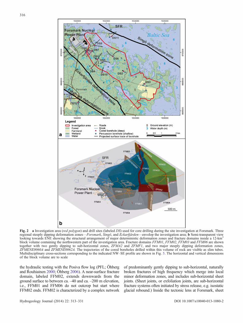
Figure 2a shows a topographic map of the Forsmark site;Forsmark is situated about 120 km north of Stockholm, inthe vicinity of the Forsmark nuclear power plant and theoffshore repository for low and intermediate level waste(SFR). The investigation area is very flat and low-lying,about 10 km2 in size. The total isostatic rebound followingthe latest deglaciation approximately 11,000 years ago is

approximately 140 m, and accounts for land uplift at acurrent rate of 6 mm/year (Söderbäck 2008). More thanhalf of the land area shown in Fig. 2a was submerged lessthan 1,000 years ago (AD 1000) and a major part of thearea currently covered by seawater in Fig. 2a is expectedto be land within about 1,000 years (AD 3000). For theapplications discussed in this report, the present-day, low-lying ground surface at the Forsmark site may beconsidered to start at the same elevation as the currentsea level, which is the Swedish Ordnance Datum. Thus, adepth of 500 m is synonymous to −500 m elevation.

Most of the rock was formed between 1.9–1.85 Ga,i.e., during Proterozoic time. The dominant rock type iscomposed of metamorphosed, medium-grained granite togranodiorite (metagranite), which has been subjected toboth ductile and brittle deformation. Three regionalsteeply dipping deformation zones, labeled Forsmark,Singö, and Eckarfjärden, envelop the investigation area,which is situated in the northwestern part of a so-calledtectonic lens in which the rock is folded and generallydisplays lower ductile strain. Figure 2a shows the locationof 25 cored boreholes and 38 percussion drilled boreholeswhich were used for multidisciplinary data acquisition.The maximum vertical depth of the cored boreholes isabout 1 km with an average of about 700 m. Thecorresponding figures for the percussion boreholes areapproximately 300 and 140 m, respectively. The informa-tion provided by reflection seismics and ground magnetics(see e.g. Juhlin and Stephens 2006) has permitted anelaborated 3D model integration of the geological,hydraulic, and chemical data acquired in the boreholes,see e.g. Follin et al. (2008b).

The structural arrangement of dominant deterministicdeformation zones and six fracture domains inside a 12-km3

block volume overlapping the northwestern part of theinvestigation area is exemplified in Fig. 2b (cf. Fig. 1b forabbreviations). The two fracture domains that constitute thepotential high-level nuclear-waste repository volume at ca. –500 m elevation are labeled FFM01 and FFM06. These aresituated in the structural footwall to the gently dipping brittledeformation zones labeled ZFMA2 and ZFMF1. FFM01 andFFM06 form the northern tip of the tectonic lens, which isaffected by a major fold structure leading to a predominanceof NE–SE-oriented deformation zones inside the lens incontrast to the NW–SW-oriented deformation zones border-ing the lens and the investigation area (Fig. 2a). FFM01 andFFM06 show a low frequency of naturally broken fractures(joints) at repository depth according to the core drilling and avery low frequency of flow-conducting fractures according to

Table 1 Terminology and guidelines for geometric properties of brittle or combined brittle and ductile structures and their recommendedhandling in the site descriptive modeling

Structure Trace length Width Handling DFN Size (radius)

Regional deformation zone > 10 km > 100 m Deterministic NALocal major deformation zone 1–10 km 5–100 m Deterministic NALocal minor deformation zone 10–1 km 0.1–5 m Stochastic 5.64–564 mFracture < 10 m < 0.1 m Stochastic < 5.64 m

NA not applicable

315


the hydraulic testing with the Posiva flow log (PFL; Öhbergand Rouhiainen 2000; Öhberg 2006). A near-surface fracturedomain, labeled FFM02, extends downwards from theground surface to between ca. –40 and ca. –200 m elevation,i.e., FFM01 and FFM06 do not outcrop but start whereFFM02 ends. FFM02 is characterized by a complex network

of predominantly gently dipping to sub-horizontal, naturallybroken fractures of high frequency which merge into localminor deformation zones, and includes sub-horizontal sheetjoints. (Sheet joints, or exfoliation joints, are sub-horizontalfracture systems often initiated by stress release, e.g. isostaticglacial rebound.) Inside the tectonic lens at Forsmark, sheet

Fig. 2 a Investigation area (red polygon) and drill sites (labeled DS) used for core drilling during the site investigation at Forsmark. Threeregional steeply dipping deformation zones—Forsmark, Singö, and Eckarfjärden—envelop the investigation area; b Semi-transparent viewlooking towards ENE showing the structural arrangement of major deterministic deformation zones and fracture domains inside a 12-km3

block volume containing the northwestern part of the investigation area. Fracture domains FFM01, FFM02, FFM03 and FFM06 are showntogether with two gently dipping to sub-horizontal zones, ZFMA2 and ZFMF1, and two major steeply dipping deformation zones,ZFMENE0060A and ZFMENE0062A. The trajectories of the cored boreholes drilled within this volume of rock are visible as slim tubes.Multidisciplinary cross-sections corresponding to the indicated NW–SE profile are shown in Fig. 5. The horizontal and vertical dimensionsof the block volume are to scale

316


joints locally exert strong directional control on groundwaterflow and contaminant transport (Follin 2008). Fracturedomain FFM03 is situated in the southeastern part of theinvestigation area in the structural hanging wall to the gentlydipping deformation zones ZFMA2 and ZFMF1, but isoutside the volume proposed for the repository. This domainis characterized by a moderate frequency of naturally brokenfractures and a low frequency of flow-conducting fractures.Fracture domains FFM04 and FFM05 coincide with the rockin close connection to the southern and northern margins ofthe tectonic lens, respectively and, thus, are influenced by theNW–SW oriented deformation zones bordering the lens andthe investigation area.

Hydrogeological DFN models have been constructedfor FFM01–FFM06, see Follin (2008) for a summary.Fracture domain FFM06 was investigated to a consider-ably lesser extent by core drilling than FFM01, but ismainly discerned from FFM01 by a minor lithologicaldifference (Stephens et al. 2007). Hence, FFM01 andFFM06 were treated as a single merged domain forpurposes of modeling in support of the integrated sitedescription. The statistical significance of the informationacquired for fracture domains FFM04 and FFM05 outsidethe target volume is very limited, 155 and 122 m ofborehole data, respectively. The vast majority of boreholedata, including over 5 km of core, is from FFM01 togetherwith several hundred meters from FFM02 and FFM03,while there is only 210 m of core in FFM06. Inconclusion, the methodology developed to constrainmodel parameters of a hydrogeological DFN model forcrystalline rock was based on data FFM01, FFM02 andFFM03, where sufficient borehole data are available forstatistical analyses. This report focuses on FFM01.

Conceptual model for fracture domains

Groundwater flow in fractured rocks takes place predom-inantly in the void space of open and partly openinterconnected fractures. Many of the hydraulic character-istics of groundwater flow through such a system can berepresented by hydrogeological DFN models, since theycan capture the characteristics of fracture geometry thatcan be observed in the field (see e.g. NRC 1996 for acomprehensive review of contemporary understanding andapplications). Flow is assumed to take place in the planeof each fracture with exchange of mass between fracturestaking place at their intersections to form a conductivenetwork in 3D. It is usually assumed that advective flowthrough the matrix between the fractures can be neglected.

Values of geological (or geometric) DFN properties,i.e., spatial arrangement of fractures in 3D, fractureorientation (strike and dip), fracture intensity in 3D, andfracture size (equivalent radius) have been interpreted atForsmark based on the geostatistical analyses of fracturedata acquired on different scales of observation, i.e.,lineament maps, outcrops, and cored boreholes (La Pointeet al. 2005; Darcel et al. 2006, 2009); Fox et al. 2007. Insummary, the framework in which fracture data has been

interpreted and a hydrogeological DFN model has beenderived is based on the following geological (geometric)concepts: (1) a Poisson process for the spatial arrangementof fractures centers in 3D; (2) Fisher distributed sets forthe orientation of fracture poles (Fisher et al. 1987); foursteeply dipping sets: NS (trend=87°, plunge=2°, kappa=22), NE (135°, 3°, 22), NW (41°, 2°, 24), and EW (190°,1°, 31) and one gently dipping set: HZ (343°, 80°, 8); and(3) power law fracture-size distributions (see the follow-ing) defined according to fracture set, fracture domain anddepth zone. These simple concepts were utilized for theintegrated site description but it is noted that alternative,more complex, models were also analyzed as part of thegeological DFN modeling (see e.g. Fox et al. 2007).

The assumption of a Poisson process to describe thespatial distribution of fractures in 3D on all scales, withoutmodification to allow for fracture termination behavior,means that fracture intensity follows Euclidean scaling, i.e.,doubling the volume would lead to a doubling of the numberof fractures. It follows that the fracture intensity–sizerelationship can be considered independently of observationscale, leading to the tectonic continuum hypothesis whichpostulates that fracture populations extend in size over a verylarge-scale range, e.g. from decimeters to kilometers (see e.g.Barton and La Pointe 1995; Davy et al. 2010). Evidence forapplying this hypothesis at the Forsmark site comes fromanalyses of fracture trace lengths, as measured on outcrops atthe smallest scale, through regional lineaments up to thelargest lineaments with lengths above 10 km (La Pointe et al.1999, 2005; Darcel et al. 2006, 2009; Fox et al. 2007). Anexample of such an analysis is illustrated in Fig. 3, whichshows density of fracture trace length per unit area foroutcrop maps at Forsmark and lineament maps in Sweden.The apparent variations in shape, from the outcrop scale onone side to the scale of Sweden on the other, address theissue of the nature of the overall transition and, in particular,the model that is likely to apply in the “window” scalebetween 10 and 100 m, bearing in mind the consideredrepository depth at Forsmark, i.e., ca. 470 m.

Power law fracture-size distributions are inherently scaleinvariant and, hence, conceptually consistent with the tectoniccontinuum hypothesis (Barton and La Pointe 1995). Forinstance, the tentative straight line shown in Fig. 3 has a slopeof kt=2 and represents a fractal self-similar model, as it ismeasured for some outcrops and most lineament maps. Thekey parameters for a power law fracture-size probability-density distribution, f(r), expressed in terms of the radius of adisc, r (m), are the shape parameter, kr, and the locationparameter, r0 (m), (see e.g. Forbes et al. 2011):

f rð Þ ¼ krr0kr

rkrþ1ð1Þ

where kr≥0 and r0>0. kr is the shape parameter forfractures in 3D space and can be estimated from thededuced shape parameter for fracture traces on 2Dsurfaces, kt, as kr=kt+1 (La Pointe 2002). The crux of

317


the developed methodology presented in this report is thetechnique used to constrain the shape parameter kr foreach fracture domain, depth zone and fracture set.

Depending on the data acquisition, f(r) is generallydefined only in a truncated range between rmin and rmax,i.e., r0≤rmin≤r≤rmax≤r1. In the low end, the scale ofobservation is limited by the diameter of the coredboreholes, which is approximately 0.076 m. This was abasis for assuming that r0≈ 0.038 m. However, twodifferent values of r0 were considered in the analyses,0.038 and 0.282 m, in order to study the important role ofthe value of the location parameter that follows fromEq. (1). The latter value was based on the lower tracelength threshold utilized in the geological mapping onoutcrops, which is approximately 0.5 m, i.e., a square witha side length of 0.5 m has the same surface area as a discof ca. 0.282-m radius. Similarly, r1 is governed by thelower trace length threshold at ground surface of thedeterministic deformations zones. As shown in Table 1,this value is ca. 1 km, which implies that r1≈ 564 m in thehydrogeological DFN modeling, i.e., a square with a sidelength of 1 km has the same surface area as a disc of ca.564 m radius.

In addition to the geological (geometric) conceptsdiscussed in the preceding, the geological characterizationof fractures in cored boreholes formed an importantframework for developing descriptions of the subset offractures relevant to the hydraulic description, i.e.,fractures that have the potential to conduct water. Threecategories of fractures were used in the geologicalcharacterization of cored boreholes based on visualinspection of drill cores and down-hole digital imaging.All naturally broken fractures were by definition regardedas “open”. Unbroken fractures with “openings” wereclassified as “partly open”, whereas unbroken fractureswithout “openings” were classified as “sealed”. In the

following, the total of broken and unbroken fractures iscalled “all fractures” and “open” refers to the sum ofbroken fractures and unbroken fractures with “open-ings”. An important subset of the “open” fractures is the“connected open fractures” (abbreviated as ‘cof’ in thefollowing) which have a potential to conduct waterdepending on the aperture (or transmissivity). Thesymbol P10 (m–1) is used to signify borehole fracturetrace frequency, i.e., number of fractures divided bylength of borehole.

In addition to the geological (geometric) classificationof fractures, flowing fractures were identified by means offlow logging based on the PFL (Öhberg and Rouhiainen2000; Öhberg 2006). The relationships between the fourfracture trace frequencies shown in Fig. 4a may be writtenas:

P10;a≥P10;o≥P10;cof ≥P10;PFL ð2Þ

where the meaning of the different subscripts (a, o, cof andPFL) is illustrated in Fig. 4a. P10,cof is of particular interestsince it refers to the frequency of open fractures that forms aconnected network, a key property of any hydrogeologicalDFNmodel. However, P10,cof cannot be measured in the field;thus, it has to be evaluated by means of DFN modeling.Concerning connectivity, it should be recognized that largefractures have higher probability of being part of a connectednetwork than small fractures (see e.g. de Marsily 1985; Bourand Davy 1997, 1998; Renshaw 1999, 2000; Darcel et al.2003). This notion is illustrated in Fig. 4b, which shows howthe probability-density functions of all, open, and flowingfractures differ for a power law fracture-size probability-density distribution. Figure 4b implies that all large fracturesare in practice also “open” and more or less flowing, whereasall small fractures are not “open” and definitely not “connectedand flowing”. The reason why P10,PFL is less than P10,cof inEq. (2) is that the PFL method has a lower measurement limit(just as any test method), which implies that not all flowingfractures could be detected (see the following). The lowermeasurement limit of the PFLmethod is sensitive to the in situconditions in each borehole (Öhberg andRouhiainen 2000). Interms of transmissivity, the typical lower measurement limit isapproximately 10–9 m2/s (see the following).

The fracture surface area per unit volume of rock,denoted as P32 (m–1), is a more versatile estimate offracture intensity than P10, which is a biased quantity offracture trace frequency since measurements along aborehole preferentially detect more fractures orthogonalto the borehole trajectory than at an oblique angle.However, P32 is impossible to measure in practice andso different modeling techniques are in use for itsestimation (e.g. Dershowitz et al. 1998; La Pointe et al.2005; Wang 2005; Fox et al. 2007). The hydrogeologicalDFN modeling described here employed the classicTerzaghi correction method (Terzaghi 1965) to derive acorrected linear fracture trace frequency P10,corr as a modelfor P32[r≥r0] for the measurable fracture categories shown

Fig. 3 Density of fracture trace length per unit area for outcropmaps at Forsmark and lineament maps of Sweden (modified afterDarcel et al. 2009)

318


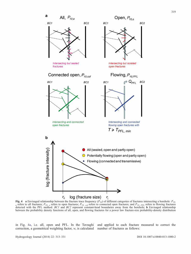
in Fig. 4a, i.e. all, open and PFL. In the Terzaghicorrection, a geometrical weighting factor, w, is calculated

and applied to each fracture measured to correct thenumber of fractures as follows:

Fig. 4 a Envisaged relationship between the fracture trace frequency (P10) of different categories of fractures intersecting a borehole: P10,

a refers to all fractures; P10, o refers to open fractures; P10, cof refers to connected open fractures; and P10, PFL refers to flowing fracturesdetected with the PFL method. BC1 and BC2 represent constant-head boundaries away from the borehole; b Envisaged relationshipbetween the probability density functions of all, open, and flowing fractures for a power law fracture-size probability-density distribution

319


w ¼ min sin αð Þ−1;wmax

n oð3aÞ

P10;corr ¼ wP10 αð Þ ð3bÞ

where α is the angle of the intersection between theborehole trajectory and the fracture plane. A maximumweight of wmax= 7 was used in the hydrogeologicalmodeling at Forsmark, equivalent to a minimum biasangle αmin of ca. 8˚.

For modeling purposes, the fracture surface area perunit volume of rock between rmin and rmax can becalculated as:

P32 rmin; rmax½ � ¼ P32 r≥r0½ � rminð Þ 2−krð Þ− rmaxð Þ 2−krð Þ

r0ð Þ 2−krð Þ

!ð4Þ

where rmin≤r≤rmax, 0<r0≤rmin, kr>2, and P32[r≥r0] is thetotal fracture intensity for all fractures greater than thechosen value of the location parameter. For rmin=r0 andrmax=r1, Eq. (4) simplifies to:

P32 r≥r1½ � ¼ P32 r≥r0½ � r0r1

� � kr−2ð Þð5Þ

where P32[r≥r1] is the fracture intensity for all fracturesgreater than r1. It follows from the power law fracture-sizeprobability-density distribution in Eq. (1) that P32[r≥r0] isalso power law distributed.

Overview of available data

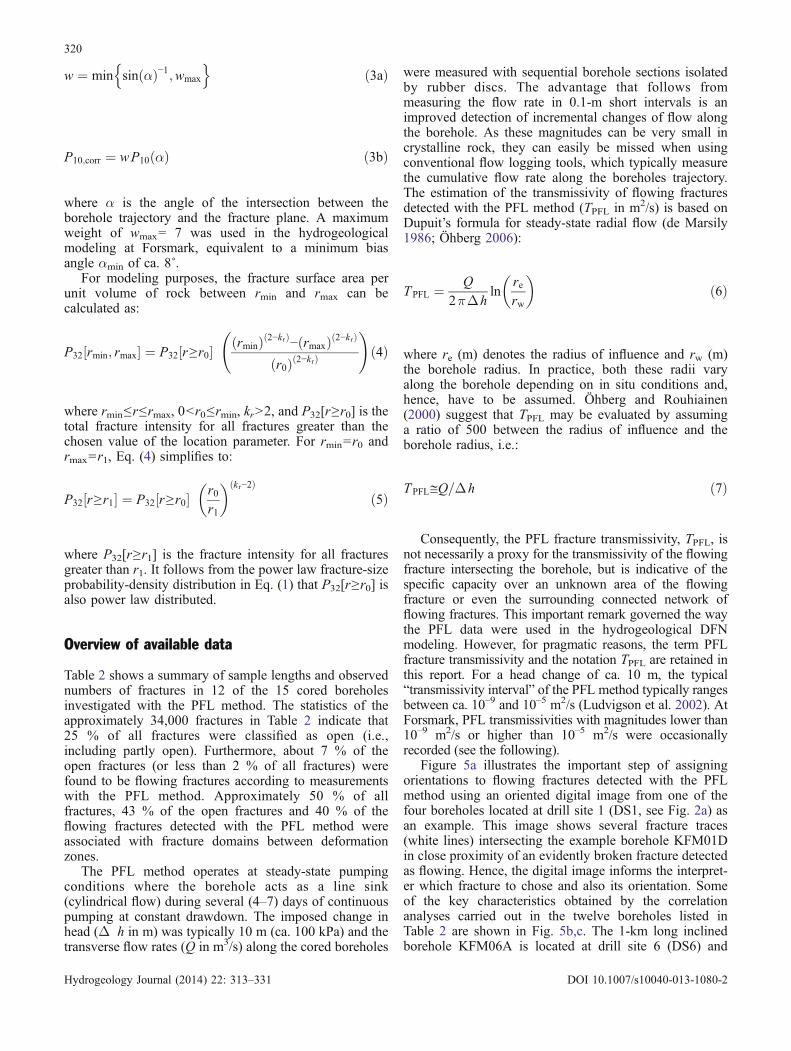
Table 2 shows a summary of sample lengths and observednumbers of fractures in 12 of the 15 cored boreholesinvestigated with the PFL method. The statistics of theapproximately 34,000 fractures in Table 2 indicate that25 % of all fractures were classified as open (i.e.,including partly open). Furthermore, about 7 % of theopen fractures (or less than 2 % of all fractures) werefound to be flowing fractures according to measurementswith the PFL method. Approximately 50 % of allfractures, 43 % of the open fractures and 40 % of theflowing fractures detected with the PFL method wereassociated with fracture domains between deformationzones.

The PFL method operates at steady-state pumpingconditions where the borehole acts as a line sink(cylindrical flow) during several (4–7) days of continuouspumping at constant drawdown. The imposed change inhead (Δ h in m) was typically 10 m (ca. 100 kPa) and thetransverse flow rates (Q in m3/s) along the cored boreholes

were measured with sequential borehole sections isolatedby rubber discs. The advantage that follows frommeasuring the flow rate in 0.1-m short intervals is animproved detection of incremental changes of flow alongthe borehole. As these magnitudes can be very small incrystalline rock, they can easily be missed when usingconventional flow logging tools, which typically measurethe cumulative flow rate along the boreholes trajectory.The estimation of the transmissivity of flowing fracturesdetected with the PFL method (TPFL in m2/s) is based onDupuit’s formula for steady-state radial flow (de Marsily1986; Öhberg 2006):

TPFL ¼ Q

2πΔhln

rerw

� �ð6Þ

where re (m) denotes the radius of influence and rw (m)the borehole radius. In practice, both these radii varyalong the borehole depending on in situ conditions and,hence, have to be assumed. Öhberg and Rouhiainen(2000) suggest that TPFL may be evaluated by assuminga ratio of 500 between the radius of influence and theborehole radius, i.e.:

TPFL≅Q=Δh ð7Þ

Consequently, the PFL fracture transmissivity, TPFL, isnot necessarily a proxy for the transmissivity of the flowingfracture intersecting the borehole, but is indicative of thespecific capacity over an unknown area of the flowingfracture or even the surrounding connected network offlowing fractures. This important remark governed the waythe PFL data were used in the hydrogeological DFNmodeling. However, for pragmatic reasons, the term PFLfracture transmissivity and the notation TPFL are retained inthis report. For a head change of ca. 10 m, the typical“transmissivity interval” of the PFL method typically rangesbetween ca. 10–9 and 10–5 m2/s (Ludvigson et al. 2002). AtForsmark, PFL transmissivities with magnitudes lower than10–9 m2/s or higher than 10–5 m2/s were occasionallyrecorded (see the following).

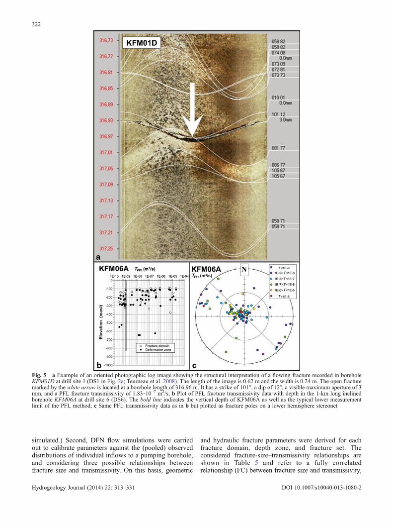
Figure 5a illustrates the important step of assigningorientations to flowing fractures detected with the PFLmethod using an oriented digital image from one of thefour boreholes located at drill site 1 (DS1, see Fig. 2a) asan example. This image shows several fracture traces(white lines) intersecting the example borehole KFM01Din close proximity of an evidently broken fracture detectedas flowing. Hence, the digital image informs the interpret-er which fracture to chose and also its orientation. Someof the key characteristics obtained by the correlationanalyses carried out in the twelve boreholes listed inTable 2 are shown in Fig. 5b,c. The 1-km long inclinedborehole KFM06A is located at drill site 6 (DS6) and

320


drilled with a NW trend, in close proximity and at a highangle to eleven possible deformation zones with an ENE–WSW or NNE–SSW trend. Six of these zones weremodeled deterministically (cf. Table 1) and the mostprominent one, ZFMENE0060A, is shown in Fig. 2b.Both KFM01A and KFM06A are located in the center ofthe tectonic lens and intersect fracture domains FFM02and FFM01. In addition, KFM06A also intersects fracturedomain FFM06. Figure 5b,c illustrates the key character-istics of the conductive fracture frequency, which are: (1)high to moderate above −150 m elevation (FFM02), (2)moderate to low in the interval −200 to −400 m elevation(FFM01), and (3) very low below −400 m elevation(FFM01 and FFM06). Further, a majority of theintersected flowing fractures in FFM02 and FFM01 aregently dipping followed by steeply dipping fractures witha NE–SW strike.

The inferred total intensities of open fractures andflowing fractures detected with the PFL method are shownfor FFM01–FFM03 in Table 3. These represent geometricmeans, i.e., data were pooled over several boreholes forthe same fracture domain. It was considered appropriate todevelop the conceptual model for flow in fractures interms of at least two depth zones, one above –400 melevation and the other below −400 m elevation (see e.g.Fig. 5b). For FFM01, a model with three depth zones wasalso attempted; above −200 m, between −200 and−400 m, and below −400 m elevation, recognizing thatFFM02 dominates the upper 200 m of rock (cf. Fig. 2b)and that there is probably an uncertainty in the position ofthese figures of about 50 m. The maximum and minimumvalues of PFL fracture transmissivity are also shown inTable 3 together with the geometric means of the pooledPFL fracture transmissivities. All these data are visualizedin Fig. 6. The spacing between open fractures andbetween flowing fractures in FFM02 is approximately0.3 and 3 m, respectively. The corresponding values aremuch larger in FFM01 situated directly beneath FFM02(cf. Fig. 2b), being approximately 2 and 200 m, respec-tively, at the proposed repository depth of about −470 m

elevation. Hence, below −400 m elevation, the flowingfractures in FFM01 are almost exclusively restricted todeformation zones (cf. Fig. 5b), symptomatic of a verysparse and poorly connected network of fracture that doesnot reach the threshold for percolation of water into thedeep rock.

Table 3 shows also bulk values of the PFL hydraulicconductivity KPFL (m/s) according to fracture domain anddepth zone. These values were obtained by calculating theproduct of the geometric mean PFL transmissivity and thegeometric mean fracture frequency and are revisited in thefollowing section dealing with up-scaling. For the sake ofcomparison, it is noted that the hydraulic conductivity ofintact rock core samples acquired in FFM01 is about 1–3orders of magnitude lower than the low value shown forFFM01 below −400 m elevation (Vilks 2007).

Table 4 shows the change in fracture intensity for open(P10,o,corr) and flowing fractures (P10,PFL,corr) according todepth zone and fracture set within FFM01. It is noted thatdata for the upper 400 m of rock are given both for asingle depth zone and for two depth zones as motivated byfield data, see Table 3 and Fig. 6. Below −400 melevation, there is only depth zone. In this depth zone,the flowing fractures in FFM01 occur within the HZ andNE sets. Besides a low frequency of conductive fractures,this depth zone is evidently also very anisotropic.

Modeling approach

The hydrogeological DFN modeling first consideredgeometrical aspects of how open-fracture-intensity sizeand orientation affect fracture-network connectivity, whichmanifests itself in borehole observations as the occurrenceof flowing fractures detected with the PFL method. Theaim of this first step was to identify viable combinations ofkr and r0 that yield the inferred intensity of flowingfractures as detected by the PFL method. (If more thanone borehole per fracture domain was available, boreholeswere pooled, i.e., one borehole per fracture domain was

Table 2 Summary of sample lengths and observed numbers of fractures in 12 of the 15 cored boreholes (KFMxxx) investigated with thePFL method. Total is equivalent to “all fractures”; hence, the sum of sealed and open fractures. The percentages shown refer to the totalnumber of fractures in each borehole. The values shown in this table are not corrected for borehole orientation bias. It is also noted that allcored boreholes tested with the PFL method are telescopic and have a steel casing in the uppermost ca. 100 m where the submersiblepumping equipment is installed

KFMxxx Cored length (m) Total No. of fractures No. of sealed fractures No. of open fractures No. of flowing fractures

KFM01A 890.82 1,517 765 (50.4 %) 752 (49.6 %) 34 (2.2 %)KFM01D 707.95 1,636 1,168 (71.4 %) 468 (28.6 %) 34 (2.1 %)KFM02A 898.82 2,199 1,756 (79.9 %) 443 (20.1 %) 104 (4.7 %)KFM03A 897.22 1,825 1,450 (79.5 %) 375 (20.5 %) 52 (2.8 %)KFM04A 875.97 4,327 2,970 (68.6 %) 1,357 (31.4 %) 71 (1.6 %)KFM05A 897.35 2,838 2,205 (77.7 %) 633 (22.3 %) 27 (1 %)KFM06A 895.16 3,680 2,864 (77.8 %) 816 (22.2 %) 99 (2.7 %)KFM07A 891.73 3,183 2,566 (80.6 %) 617 (19.4 %) 26 (0.8 %)KFM07C 400.05 1,765 1,480 (83.9 %) 285 (16.1 %) 14 (0.8 %)KFM08A 846.31 4,268 3,555 (83.3 %) 713 (16.7 %) 41 (1 %)KFM08C 846.70 4,198 3,522 (83.9 %) 676 (16.1 %) 21 (0.5 %)KFM10A 437.12 2,755 1,756 (63.7 %) 999 (36.3 %) 54 (2 %)Total 9,485.20 34,191 26,057 (76.2 %) 8,134 (23.8 %) 577 (1.7 %)

321


simulated.) Second, DFN flow simulations were carriedout to calibrate parameters against the (pooled) observeddistributions of individual inflows to a pumping borehole,and considering three possible relationships betweenfracture size and transmissivity. On this basis, geometric

and hydraulic fracture parameters were derived for eachfracture domain, depth zone, and fracture set. Theconsidered fracture-size–transmissivity relationships areshown in Table 5 and refer to a fully correlatedrelationship (FC) between fracture size and transmissivity,

Fig. 5 a Example of an oriented photographic log image showing the structural interpretation of a flowing fracture recorded in boreholeKFM01D at drill site 1 (DS1 in Fig. 2a; Teurneau et al. 2008). The length of the image is 0.62 m and the width is 0.24 m. The open fracturemarked by the white arrow is located at a borehole length of 316.96 m. It has a strike of 101°, a dip of 12°, a visible maximum aperture of 3mm, and a PFL fracture transmissivity of 1.83·10–7 m2/s; b Plot of PFL fracture transmissivity data with depth in the 1-km long inclinedborehole KFM06A at drill site 6 (DS6). The bold line indicates the vertical depth of KFM06A as well as the typical lower measurementlimit of the PFL method; c Same PFL transmissivity data as in b but plotted as fracture poles on a lower hemisphere stereonet

322


a semi-correlated relationship (SC), and an uncorrelatedrelationship (UC).

Of the 12 cored boreholes analyzed, four are essentiallyvertical, while the others are inclined at 60˚ to thehorizontal, mostly dipping toward approximately NW orNE. Most boreholes are 1 km long, but have a steel casingin the top 100 m (Table 2). One of the issues dealt with inthe data compilation was how to combine data fromboreholes of different trajectory so as to avoid bias causedby the preferential sampling of fractures oriented orthog-onal to the borehole axis. The approach used was tocollate statistics using the Terzaghi weighting in Eq. (3) to

correct for the bias. Similarly, the simulated fracturefrequencies are also corrected using Terzaghi weightings.In conclusion, the hydrogeological DFN modeling pre-sented in this report was based on geometric and hydraulicproperties homogenized over the fracture domains, so asto derive models that capture the overall geometric andhydraulic characteristics of each fracture domain, depthzone, and fracture set without conditioning the localfracture position and flows around each borehole. Hence,the derived DFN models might be considered as spatiallyunconditioned stochastic models appropriate to eachfracture domain and depth zone. The methodology andthe results are presented in the following using measureddata and simulations for fracture domain FFM01.

Step 1: calibration of power law parameters

The methodology used to derive optimal power lawparameters kr and r0 for open fractures involved thefollowing steps: (1) DFN realizations representing fourdifferent power law models for fracture size (see thefollowing) were generated inside a model domain centeredaround a 1-km long vertical borehole (scan line). Byspecification, each DFN realization mimicked the intensi-ties of open fractures, P10,o,corr, shown in Table 4; (2) eachDFN realization was subjected to a connectivity analysisbetween the boundaries of the model domain and theintensity of connected open fractures for each fracture-sizemodel was calculated to assess which best reproduced theintensity of flowing fractures as detected by the PFLmethod, P10,PFL,corr; (3) the shape parameter kr of eachfracture set of the best fracture-size model was optimizedto give the best match possible of the intensity ofconnected open fractures against the flowing fracturesdetected with the PFL method. This procedure wasrepeated for each fracture domain and depth zone.

The following power law size-distribution models wereconsidered based on the range of size distributionparameters indicated by (1) the analysis of lineament tracedata conducted at three sites in the Fennoscandian Shield(La Pointe et al. 1999), and (2) the sensitivity analysis onfracture connectivity derived by means of numericalsimulations (Follin et al. 2005):

Table 3 Geometric mean fracture intensity of open fractures (<P10, o,corr>) and flowing fractures detected with the PFL method (<P10,

PFL,corr>) for three depth zones in fracture domains FFM01–FFM03. Maximum and minimum values of PFL fracture transmissivity (TPFL)in each fracture domain and depth zone are also shown together with the geometric means (<TPFL>) and PFL hydraulic conductivity(KPFL=<TPFL><P10,PFL,corr>). Italic numbers are plotted in Fig. 6

Parameter Fracture domain and (depth zone)FFM02 FFM01 FFM01 FFM01 FFM03 FFM03(≥ –200 m) (≥ –200 m) (−200 to −400 m) (< −400 m) (≥ –400 m) (< −400 m)

<P10,o,corr> (m–1) 3.17 1.13 1.02 0.535 1.10 0.77<P10,PFL,corr> (m–1) 0.33 0.153 0.041 0.005 0.09 0.05Max TPFL (m2/s) 7.3·10–6 1.9·10–7 1.8·10–7 8.9·10–8 6.8·10–7 1.9·10–7

Min TPFL (m2/s) 2.4·10–10 2.5·10–10 2.7·10–10 6.2·10–10 1.9·10–9 1.1·10–9

<TPFL> (m2/s) 1.0·10–8 6.9·10–9 2.4·10–9 6.5·10–9 3.6·10–8 1.5·10–8

KPFL (m/s) 3.3·10–9 1.1·10–9 9.6·10–11 3.3·10–11 3.2·10–9 7.2·10–10

Fig. 6 Variation with depth for the key fracture domains in thearea coinciding with DS1-5-6-8-7 in Fig. 2a; a Fracture intensities(fractures per km) P10,o,corr and P10,PFL,corr; b PFL fracturetransmissivity TPFL. Solid lines represent geometric means over allboreholes intersecting and dashed lines represent the minimum andmaximum values. Bold values are those highlighted in Table 3

323


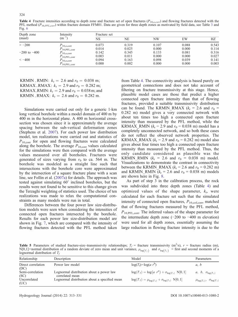
KRMIN RMIN: kr ¼ 2:6 and r0 ¼ 0:038 m;KRMAX RMAX: kr ¼ 2:9 and r0 ¼ 0:282 m;KRMAX RMIN: kr ¼ 2:9 and r0 ¼ 0:038m; andKRMIN RMAX: kr ¼ 2:6 and r0 ¼ 0:282 m:

Simulations were carried out only for a generic 1-kmlong vertical borehole within a model domain of 400 m by400 m in the horizontal plane. A 400 m horizontal cross-section was chosen since it is approximately the averagespacing between the sub-vertical deformation zones(Stephens et al. 2007). For each power law distributionmodel, ten realizations were carried out and statistics ofP10,corr for open and flowing fractures were calculatedalong the borehole. The average P10,corr values calculatedfor the simulations were then compared with the averagevalues measured over all boreholes. Fractures weregenerated of sizes varying from r0 to ca. 564 m. Theborehole was modeled as a straight line such thatintersections with the borehole core were approximatedby the intersection of a square fracture plane with a scanline, see Follin et al. (2007a) for details. The approach wastested against simulating 60˚ inclined boreholes, but theresults were not found to be sensitive to this change giventhe Terzaghi weighting of statistics used. The choice of tenrealizations was made to relax the computational con-straints as many models were run in total.

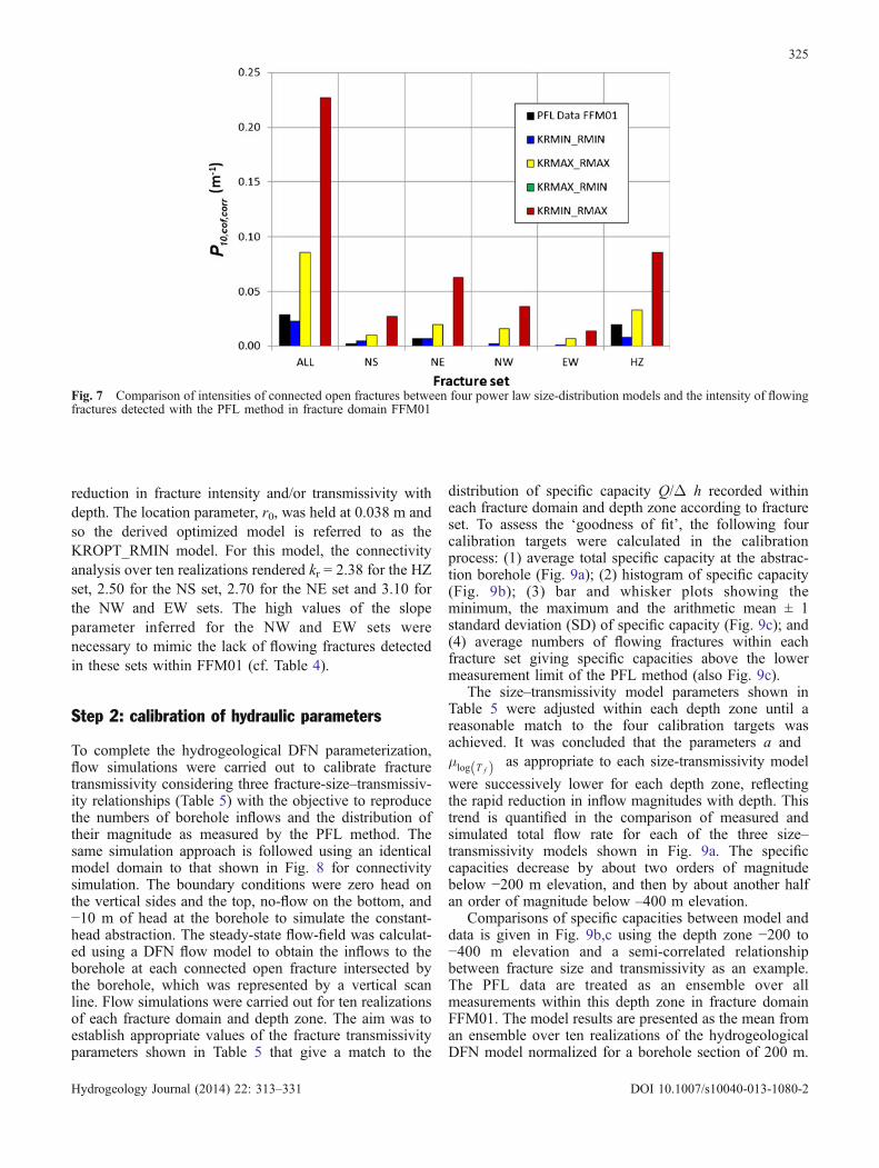
Differences between the four power law size-distribu-tion models were seen when considering the intensities ofconnected open fractures intersected by the borehole.Results for each power law size-distribution model areshown in Fig. 7, which are compared with the intensity offlowing fractures detected with the PFL method taken

from Table 4. The connectivity analysis is based purely ongeometrical connections and does not take account offiltering on fracture transmissivity at this stage. Hence,plausible model cases are those that predict a higherconnected open fracture intensity than that of flowingfractures, provided a suitable transmissivity distributioncan be found. The KRMIN_RMAX (kr = 2.6 and r0 =0.282 m) model gives a very connected network withabout ten times too high a connected open fractureintensity than measured by the PFL method, while theKRMAX_RMIN (kr = 2.9 and r0 = 0.038 m) model has acompletely unconnected network, and so both these casesdo not reflect the observed network properties. TheKRMAX_RMAX (kr = 2.9 and r0 = 0.282 m) model alsogives about four times too high a connected open fractureintensity than measured by the PFL method. Thus, theonly candidate considered as plausible was theKRMIN_RMIN (kr = 2.6 and r0 = 0.038 m) model.Visualizations to demonstrate the contrast in connectivitybetween the KRMIN_RMAX (kr = 2.6 and r0 = 0.282 m)and KRMIN_RMIN (kr = 2.6 and r0 = 0.038 m) modelsare shown here in Fig. 8.

As part of step 3 in the calibration process, the rockwas subdivided into three depth zones (Table 4) andoptimized values of the shape parameter, kr, werecalculated for each fracture set such that the simulatedintensity of connected open fractures, P10,cof,corr, matchedthat of flowing fractures measured by the PFL method,P10,PFL,corr. The inferred values of the shape parameter forthe intermediate depth zone (−200 to −400 m elevation)were used for all depth zones, essentially assuming thelarge reduction in flowing fracture intensity is due to the

Table 4 Fracture intensities according to depth zone and fracture set of open fractures (P10,o,corr) and flowing fractures detected with thePFL method (P10,PFL,corr) within fracture domain FFM01. Data are given for three depth zones as motivated by field data, see Table 3 andFig. 6

Depth zone(masl)

Intensity(m–1)

Fracture setNS NE NW EW HZ

> −200 P10,o,corr 0.073 0.319 0.107 0.088 0.543P10,PFL,corr 0.014 0.025 0.000 0.000 0.114

−200 to −400 P10,o,corr 0.142 0.345 0.133 0.081 0.316P10,PFL,corr 0.003 0.011 0.000 0.000 0.027

< −400 P10,o,corr 0.094 0.163 0.098 0.039 0.141P10,PFL,corr 0.000 0.002 0.000 0.000 0.003

Table 5 Parameters of studied fracture-size–transmissivity relationships; Tf = fracture transmissivity (m2/s), r = fracture radius (m),N[0,1]=normal distribution of a random deviate of zero mean and unit variance, μlog T fð Þ and σlog T fð Þ = first and second moments of alognormal distribution of Tf

Relationship Description Model Parameters

Direct correlation(DC)

Power law model log(Tf)=log(a rb) a, b

Semi-correlation(SC)

Lognormal distribution about a power lawcorrelated mean

log T fð Þ ¼ log a rb� �þ σlog T fð Þ N 0; 1½ � a; b; σlog T fð Þ

Uncorrelated(UC)

Lognormal distribution about a specified mean log T fð Þ ¼ μlog T fð Þ þ σlog T fð Þ N 0; 1½ � μlog T fð Þ; σlog T fð Þ

324


reduction in fracture intensity and/or transmissivity withdepth. The location parameter, r0, was held at 0.038 m andso the derived optimized model is referred to as theKROPT_RMIN model. For this model, the connectivityanalysis over ten realizations rendered kr = 2.38 for the HZset, 2.50 for the NS set, 2.70 for the NE set and 3.10 forthe NW and EW sets. The high values of the slopeparameter inferred for the NW and EW sets werenecessary to mimic the lack of flowing fractures detectedin these sets within FFM01 (cf. Table 4).

Step 2: calibration of hydraulic parameters

To complete the hydrogeological DFN parameterization,flow simulations were carried out to calibrate fracturetransmissivity considering three fracture-size–transmissiv-ity relationships (Table 5) with the objective to reproducethe numbers of borehole inflows and the distribution oftheir magnitude as measured by the PFL method. Thesame simulation approach is followed using an identicalmodel domain to that shown in Fig. 8 for connectivitysimulation. The boundary conditions were zero head onthe vertical sides and the top, no-flow on the bottom, and−10 m of head at the borehole to simulate the constant-head abstraction. The steady-state flow-field was calculat-ed using a DFN flow model to obtain the inflows to theborehole at each connected open fracture intersected bythe borehole, which was represented by a vertical scanline. Flow simulations were carried out for ten realizationsof each fracture domain and depth zone. The aim was toestablish appropriate values of the fracture transmissivityparameters shown in Table 5 that give a match to the

distribution of specific capacity Q/Δ h recorded withineach fracture domain and depth zone according to fractureset. To assess the ‘goodness of fit’, the following fourcalibration targets were calculated in the calibrationprocess: (1) average total specific capacity at the abstrac-tion borehole (Fig. 9a); (2) histogram of specific capacity(Fig. 9b); (3) bar and whisker plots showing theminimum, the maximum and the arithmetic mean ± 1standard deviation (SD) of specific capacity (Fig. 9c); and(4) average numbers of flowing fractures within eachfracture set giving specific capacities above the lowermeasurement limit of the PFL method (also Fig. 9c).

The size–transmissivity model parameters shown inTable 5 were adjusted within each depth zone until areasonable match to the four calibration targets wasachieved. It was concluded that the parameters a andμlog T fð Þ as appropriate to each size-transmissivity model

were successively lower for each depth zone, reflectingthe rapid reduction in inflow magnitudes with depth. Thistrend is quantified in the comparison of measured andsimulated total flow rate for each of the three size–transmissivity models shown in Fig. 9a. The specificcapacities decrease by about two orders of magnitudebelow −200 m elevation, and then by about another halfan order of magnitude below –400 m elevation.

Comparisons of specific capacities between model anddata is given in Fig. 9b,c using the depth zone −200 to−400 m elevation and a semi-correlated relationshipbetween fracture size and transmissivity as an example.The PFL data are treated as an ensemble over allmeasurements within this depth zone in fracture domainFFM01. The model results are presented as the mean froman ensemble over ten realizations of the hydrogeologicalDFN model normalized for a borehole section of 200 m.

Fig. 7 Comparison of intensities of connected open fractures between four power law size-distribution models and the intensity of flowingfractures detected with the PFL method in fracture domain FFM01

325


Fig. 8 Visual comparison of simulated connected open fractures for the very connected KRMIN_RMAX model (left column) and thepoorly connected KRMIN_RMIN model (right column) around a vertical borehole in fracture domain FFM01. Top row: 3D plots of allconnected open fractures. Bottom row: a vertical slice through the same networks. Fractures are colored by fracture set

326


Figure 9b shows a histogram over all sets and Fig. 9cshows a bar and whisker plot for individual sets. Thenumbers alongside the bars in Fig. 9c represent thenumbers of inflows per 200 m of borehole correspondingto each set above the detection limit. The detection limit ishere assumed to be the minimum PFL fracture transmis-sivity measured in the modeled volume (2.5·10–10 m2/sfor FFM01, cf. Fig. 5b and Table 3). Figure 9c shows thatthe inflows are dominated by the HZ set with contributionfrom the NS and NE sets, whereas the NW and EW setsmake no contribution. To illustrate how the derived size–transmissivity models compare, they are plotted here aslog–log plots in Fig. 9d for the depth zone −200 to−400 m elevation. The semi-correlated and fully correlat-ed relationships follow similar trends and also interceptthe uncorrelated model for fractures of about 10 m radius.This is perhaps to be expected since fractures around 10–100 m are the ones that form the connected network

giving inflows in the simulations. In other words, the flowrate to/from an abstraction/injection borehole in ahydrogeological DFN is probably largely controlled byhow well connected the network of open fractures is (i.e.largely determined by size and intensity). This hypothesisis reinforced by the findings by Öhman and Follin (2010),who studied the role of “hydraulic chokes” in ahydrogeological DFN where all fractures had the sametransmissivity regardless of fracture size. Öhman andFollin (2010) concluded that in a sparely fracturedcrystalline rock, the extent of the geometric contactbetween two transmissive fractures is crucial for the flowacross the contact area; i.e., if the geometric contact wassmall relative to the size of the two intersecting fractures,a “hydraulic choke” occurred.

The results of the hydrogeological DFN simulations forForsmark can be summarized in the simplest terms in thatthe key aspect of the Forsmark site is that the target

Fig. 9 Comparison of flow data acquired with PFL method in cored boreholes within fracture domain FFM01 and average flow data overten DFN realizations using the calibrated KROPT_RMIN model and three fracture size–transmissivity models (labeled FC, SC and UC, seeTable 5): a Average total inflow divided by head change (drawdown) for each transmissivity model and depth zone; b Histogram of theaverage specific capacity for the SC model and the intermediate depth zone; c Bar and whisker plots of the specific capacity according tofracture set for the SC model and the intermediate depth zone, and average number of flowing fractures per 200 m of borehole; and dInferred-size–transmissivity relationships for each transmissivity model and the intermediate depth zone

327


fracture domain (FFM01) shows very strong variationswith depth, and so the hydrogeological DFN model hasbeen split into three layers: above −200 m, between −200and −400 m, and below −400 m elevation. This domain isalso very anisotropic, being dominated by the HZ set, andonly a small contribution from the NE and sometimes NSsets, whereas the NW and EW set make no contribution.Indeed, below −400 m elevation there are only two flow-conductive fracture sets, HZ and NE, implying stronganisotropy and the network of connected open fracturesapparently being compartmentalized and close to thepercolation threshold. This observation is supported bythe ca. 200 unbroken 3-m long drill cores abstractedduring core drilling. Further, by analyzing the measuredPFL flow logs run prior to pumping, it is concluded thatthe boreholes drilled in Forsmark increase the connectivityof the flowing fracture network. This is evident from thedistribution of inflows and outflows observed along thecored boreholes when these were held open and at restprior to pumping.

Equivalent hydraulic conductivities

A hydrogeological DFN model is formulated in terms of astatistical recipe for each attribute of discrete fractures,and can be demonstrated to mimic many statisticalcharacteristics of discrete flows as measured by the PFLmethod. However, it is also of interest to consider the bulkflow properties implied by the DFN in terms of anequivalent hydraulic conductivity tensor, which is a morewidely understood parameterization of hydrogeologicalproperties. The conversion between a DFN parameteriza-tion and an equivalent continuous porous medium(ECPM) can be described as up-scaling fracture flowproperties to bulk flow properties. The up-scaling is mostaccurately achieved using a flux-based approach, wherethe flow through a sub-volume of a fracture network iscalculated under various boundary conditions. The output

is a hydraulic conductivity tensor that reproduces the setof simulated flows through the volume. The flux-basedup-scaling method used here is described in Jackson et al.(2000). A full six-component symmetric tensor is calcu-lated, and diagonalized into principal components. For thepresentation here, an overall effective hydraulic conduc-tivity, Keff (m/s) expressed as the geometric mean of thethree principal components, is used. The equivalenthydraulic conductivity is scale dependent, and so iscalculated on 5, 20 and 100-m scales, coincident withthe scale of intervals on which double-packer injectiontests, labeled PSS, were carried out. For the model,hydraulic conductivities were calculated on a 10 by 10by 10 grid of blocks for each scale to provide statistics ofthe geometric mean and standard deviation in log10(Keff)as well as the number of blocks that contained networksthat percolated the volume. The simulation results arecompared with the PSS data in Fig. 10 for the three scalesand three depth zones. As a further comparison, estimatesof effective hydraulic conductivity are made utilizing thePFL data in two ways: (1) by calculating the product ofthe geometric mean PFL transmissivity and the geometricmean fracture frequency (cf. Table 3) for each depth zone,and (2) by calculating the total inferred transmissivity ofthe FPL method divided by total borehole length withineach depth zone. It is seen in Fig. 10 that the 20 and 100-m-scale PSS data tend to fall within these two PFL-basedestimates, except below −400 m elevation where therewere so few measurements above the detection limit ofeither method to make only qualitative comparisonspossible. The mean simulated values also fall betweenthese two PFL-based estimates for all block scales, asmight be expected, since the DFN was calibrated againstthe same PFL data. The variability in effective hydraulicconductivity and percentage of blocks/intervals thatconduct water for the various scales is also ratherconsistent between simulations and the PSS data.

These comparisons provide confidence that the derivedDFN formulation of detailed flows within individual

Fig. 10 Comparison of up-scaled effective hydraulic conductivities according to depth zone for 5, 20 and 100-m model blocks predictedby the hydrogeological DFN model for fracture domain FFM01 and: (1) hydraulic conductivities from 5, 20 and 100-m-long test sectionsusing double packer injection tests (labeled PSS) within each depth zone; (2) KPFL=<TPFL><P10, PFL,corr> within each depth zone (cf.Table 3); and (3) the total transmissivity inferred by the PFL method divided by total borehole length within each depth zone. Thepercentages at the base of some of the bars indicate the fraction of blocks (for the model) or borehole sections (for the data) that conductwater. The error bars indicate 1 SD in the common logarithm of the corresponding effective hydraulic conductivity

328


fractures is also suited to simulating mean bulk-flowproperties and their spatial variability. The equivalentcontinuous porous medium (ECPM) approach was used inthe site-scale groundwater-flow modeling carried out insupport of the integrated site description at the Forsmarksite (Follin et al. 2007b; Follin 2008). Since each (ECPM)model was based on a particular underlying stochasticDFN realization, the ECPM models were also stochastic,which required multiple realizations (Follin et al. 2008a;Follin 2008). Hartley and Joyce (2013) provide anoverview of the computational issues dealt with duringthe up-scaling from a DFN to an ECPM.

Conclusions

A methodology has been developed for constraining thegeometric and hydraulic parameters that define ahydrogeological DFN model intended for site-scalegroundwater flow and solute transport modeling insparsely fractured crystalline rock. It is based on detailedflow logging and down-hole digital imaging in coredboreholes in combination with multiple DFN realizations,fracture connectivity analysis and pumping test simula-tions. The advantage that follows from measuring the flowrate in 0.1-m short intervals is an improved detection ofincremental changes of flow along the borehole. As thesemagnitudes can be very small in crystalline rock, they caneasily be missed when using conventional flow loggingtools, which typically measure the cumulative flow ratealong the boreholes trajectory. In combination withfracture orientations determined by down-hole digitalimaging, the incremental flows provide a unique opportu-nity to model fracture spatial intensity and anisotropicconnectivity of conductive fracture networks in sparselyfractured crystalline rock.

The methodology is demonstrated using measured dataand simulations for one of the crystalline rock sitesproposed for a high-level nuclear waste repository inSweden, Forsmark, which have been investigated andcharacterized by the Svensk Kärnbränslehantering AB.The large-scale geological structure of the crystalline rockat the Forsmark site has been classified in terms ofdeformation zones of elevated fracture frequency. Therock between deformation zones was divided into fracturedomains according to different fracture frequency. Thehydrogeological DFN modeling carried out in support ofan integrated site description for the Forsmark site wasbased on geometric and hydraulic properties homogenizedover the fracture domains, so as to derive models thatcapture the overall geometric and hydraulic characteristicsof each fracture domain, depth zone, and fracture setwithout conditioning the local fracture position and flowsaround each borehole. Hence, the derived hydrogeologicalDFN models might be considered as spatially uncondi-tioned stochastic models appropriate to each fracturedomain and depth zone.

The key fracture property governing fracture connec-tivity in sparsely fractured crystalline rock is fracture size.

The crux of the developed methodology is the techniqueused to constrain the size-distribution parameters for eachfracture domain, depth zone and fracture set to matchmeasured inflows to cored boreholes investigated bydetailed flow logging using the Posiva flow log (PFL).The simulations carried out for the Forsmark site suggestthat a good match could be obtained for a power law sizedistribution where the value of the location parameterequals the borehole radius but with different values for theshape parameter, depending on fracture domain andfracture set.

The so-called PFL fracture transmissivity is notnecessarily a proxy for the transmissivity of the flowingfracture intersecting the borehole, but indicative of thespecific capacity over an unknown area of the flowingfracture or even the surrounding connected network offlowing fractures. Hence, different relationships betweenfracture size and fracture transmissivity were studied bymeans of numerical modeling. The considered alternativefracture-size–transmissivity relationships were a fullycorrelated relationship (FC) between fracture size andtransmissivity, a semi-correlated relationship (SC), and anuncorrelated relationship (UC). The parameters for eachsize-transmissivity relationship were calibrated against themeasured flow rates gathered from the hydraulic testingwith the PFL method. All three relationships give similarranges of transmissivity for fractures in the size range 10–100 m. This is perhaps to be expected since fracturesaround 10–100 m are the ones that typically form theconnected network giving inflows in the simulations.Notwithstanding, if one relationship is to be used overthe others, the intuitive choice would be the semi-correlated relationship, since a high transmissivity gener-ally implies a large “radius of influence”, but, due tofracture heterogeneities, not necessarily a fully correlatedrelationship.

It is also of interest to consider what bulk flowproperties the hydrogeological DFN model implies interms of an up-scaled, equivalent hydraulic conductivitytensor, which is a more widely understood representationof permeability, e.g. in site-scale groundwater flowmodeling. Comparisons with the scale of intervals onwhich double-packer injection tests were carried outprovide confidence that the derived DFN formulation ofdetailed flows within individual fractures is also suited tosimulating mean bulk flow properties and their spatialvariability in site-scale groundwater-flow modeling.

Acknowledgements This report was possible due to the significantfield work conducted on behalf of the Svensk KärnbränslehanteringAB. (SKB) during the site investigation for a geological repositoryfor high-level nuclear waste at the Forsmark site. We would like tothank those who contributed to the extensive data collection and/oranalysis including: M. Stephens, A. Simeonov, J. Petersson, and J.Levén. Finally, we would like to thank J.-O. Selroos and thereviewers for their helpful comments and suggestions, whichimproved the quality of the manuscript.All SKB reports referred to in this report, as well as the underlyingdata reports, can be downloaded from the SKB website—http://www.skb.se/; click on “Publications”, and then enter the reportnumber, e.g. “R-07-45”.

329


http://www.skb.se/

http://www.skb.se/

References

Andersson J, Skagius K, Winberg A, Ström A, Lindborg T (2007)Site descriptive modeling as a part of site characterisation inSweden: concluding the surface based investigations. Paperpresented at the 11th Int. Conf. on Environmental Remediationand Radioactive Waste Management (ICEM2007), Bruges,Belgium, 2–6 September 2007

Andersson J, Skagius K, Winberg A, Lindborg T, Ström A (2013)Site descriptive modeling for a final repository for spent nuclearfuel in Sweden. Environ Earth Sci 69(3):1045–1060.doi:10.1007/s12665-013-2226-1

Barton CC, La Pointe PR (1995) Fractals in the earth sciences.Plenum, New York

Bath A, Lalieux P (1999) Technical summary of the SEDEWorkshop on the use of hydrogeochemical information intesting groundwater flow models. In: Use of hydrogeochemicalinformation in testing groundwater flow models, Technicalsummary and proceedings of an NEA Workshop, Borgholm,Sweden, 1–3 September 1997. Coordinating Group on SiteEvaluation and Design of Experiments for Radioactive WasteDisposal – SEDE, OECD-NEA, Paris

Bour O, Davy P (1997) Connectivity of random fault networksfollowing a power law fault length distribution. Water ResourRes 33(7):1567–1584. doi:10.1029/96WR00433

Bour O, Davy P (1998) On the connectivity of three‐dimensionalfault networks. Water Resour Res 34(10):2611–2622.doi:10.1029/98WR01861

Darcel C, Bour O, Davy P, de Dreuzy JR (2003) Connectivityproperties of two‐dimensional fracture networks with stochasticfractal correlation. Water Resour Res 39(10):1272. doi:10.1029/2002WR001628

Darcel C, Davy P, Bour O, de Dreuzy J R (2006) Discrete fracturenetwork for the Forsmark site. SKB R-06-79, SvenskKärnbränslehantering AB, Stockholm

Darcel C, Davy P, Le Goc R, de Dreuzy JR, Bour O (2009)Statistical methodology for discrete fracture model: includingfracture size, orientation uncertainty together with intensityuncertainty and variability. SKB R-09-38, SvenskKärnbränslehantering AB, Stockholm

Davy P, Le Goc R, Darcel C, Bour O, de Dreuzy JR, Munier R(2010) A likely universal model of fracture scaling and itsconsequence for crustal hydromechanics. J Geophys Res115:B10411. doi:10.1029/2009JB007043

de Marsily G (1985) Flow and transport in fractured rocks:connectivity and scale effect. Proc. of the 17th Int. IAH Cong.on Hydrology of Rocks of Low Permeability, Tucson, AZ,January 1985, pp 267–277

de Marsily G (1986) Quantitative hydrogeology: groundwaterhydrology for engineers. Academic, London

Dershowitz WS, La Pointe PR, Cladouhos T (1998) Derivation offracture spatial pattern parameters from borehole data. Int JRock Mech Min Sci 35(4):508–508. doi:10.1016/S0148-9062(98)00149-1

Fisher N, Lewis T, Embleton B (1987) Statistical analysis ofspherical data. Cambridge University Press, Cambridge, UK

Follin S (2008) Bedrock hydrogeology Forsmark, Site descriptivemodelling, SDM-Site Forsmark. SKB R-08-95, SvenskKärnbränslehantering AB, Stockholm

Follin S, Stigsson M, Svensson U, (2005) Regional hydrogeologicalsimulations for Forsmark: numerical modelling usingDarcyTools—preliminary site description Forsmark area, version1.2. SKB R-05-60, Svensk Kärnbränslehantering AB, Stockholm

Follin S, Levén J, Hartley L, Jackson P, Joyce S, Roberts D, Swift B(2007a) Hydrogeological characterisation and modelling ofdeformation zones and fracture domains: Forsmark modellingstage 2.2. SKB R-07-48, Svensk Kärnbränslehantering AB,Stockholm

Follin S, Johansson P-O, Hartley L, Jackson P, Roberts D, Marsic N(2007b) Hydrogeological conceptual model development andnumerical modelling using ConnectFlow: Forsmark modelling

stage 2.2. SKB R-07-49, Svensk Kärnbränslehantering AB,Stockholm

Follin S, Hartley L, Jackson P, Roberts D, Marsic N (2008a)Conceptual model development and numerical modelling usingConnectFlow: Forsmark modelling stage 2.3. SKB R-08-23,Svensk Kärnbränslehantering AB, Stockholm

Follin S, Stephens MB, Laaksoharju M, Nilsson A-C, Smellie JAT,Tullborg E-L (2008b) Modelling the evolution of hydrochemicalconditions in the Fennoscandian Shield during Holocene timeusing multidisciplinary information. Appl Geochem 23(7):2004–2020. doi:10.1016/j.apgeochem.2008.02.022

Forbes C, Evans M, Hastings N, Peacock B (2011) Statisticaldistributions, 4th edn. Wiley, Hoboken, NJ

Fox A, La Pointe PR, Hermanson J, Öhman J (2007) Statisticalgeological discrete fracture networkmodel: Forsmarkmodelling stage2.2. SKB R-07-46, Svensk Kärnbränslehantering AB, Stockholm

Hartley L, Joyce S (2013) Approaches and algorithms forgroundwater flow modeling in support of site investigationsand safety assessment of the Forsmark site, Sweden. J Hydrol.doi:10.1016/j.jhydrol.2013.07.031

IAEA (1999) Hydrogeological investigations of sites for thegeological disposal of radioactive waste. Technical report 391,International Atomic Energy Agency, Vienna

Jackson P, Hoch A, Todman S (2000) Self-consistency of aheterogeneous continuum porous medium representation of afractured medium. Water Resour Res 36(1):189–202.doi:10.1029/1999WR900249

Juhlin C, Stephens MB (2006) Gently dipping fracture zones inPaleoproterozoic metagranite, Sweden: evidence from reflectionseismic and cored borehole data and implications for thedisposal of nuclear waste. J Geophys Res 111:B09302.doi:10.1029/2005JB003887

Koistinen T, Stephens MB, Bogatchev V, Nordgulen Ø, WennerströmM, Korhonen J (2001) Geological map of the FennoscandianShield, scale 1:2,000,000. Geological Surveys of Finland (Espoo),Norway (Trondheim), Sweden (Uppsala) and the North-WestDepartment of Natural Resources of Russia (Joensuu)

La Pointe PR (2002) Derivation of parent fracture populationstatistics from trace length measurements for fractal fracturepopulations. Int J Rock Mech Min Sci 39:381–388

La Pointe PR, Cladouhos T, Follin S (1999) Calculation ofdisplacements on fractures intersecting canisters induced byearthquakes: Aberg, Beberg and Ceberg examples. SKB TR-99-03, Svensk Kärnbränslehantering AB, Stockholm

La Pointe PR, Olofsson I, Hermanson J (2005) Statistical model offractures and deformation zones for Forsmark: preliminary sitedescription Forsmark area, version 1.2. SKB R-05-26, SvenskKärnbränslehantering AB, Stockholm

Ludvigson J-E, Hansson K, Rouhiainen P (2002) Methodologystudy of Posiva difference flow meter in borehole KLX02 atLaxemar. SKB R-01-52, Svensk Kärnbränslehantering AB,Stockholm

Milnes AG, Stephens MB, Wahlgren C-H, Wikström L (2008)Geoscience and high-level nuclear waste disposal: the Nordicscene. Episodes 31(1):168–175

NRC (1996) Rock fractures and fluid flow: contemporary under-standing and applications. National Research Council, NationalAcademy Press, Washington, DC

OECD-NEA (1993) Paleo-hydrogeological methods and their applica-tion. Technical summary and proceedings of a NEA Workshop,Paris, 9–10 November 1992, Coordinating Group on Site Evalua-tion and Design of Experiments for Radioactive Waste Disposal –SEDE, Organization for Economic Co-operation and Development-Nuclear Energy Agency, OECD-NEA, Paris

Öhberg A (2006) Investigation methods and equipment used by Posiva.Posiva technical report WR 2006–81, Posiva, Eurajoki, Finland

Öhberg A, Rouhiainen PR (2000) Posiva groundwater flowmeasuring techniques. Posiva technical report WR 2000–12,Posiva, Eurajoki, Finland

Öhman J, Follin S (2010) Hydrogeological modelling of SFR: modelversion 0.2. SKB R-10-03, Svensk Kärnbränslehantering AB,Stockholm

330


http://dx.doi.org/10.1007/s12665-013-2226-1

http://dx.doi.org/10.1029/96WR00433

http://dx.doi.org/10.1029/98WR01861

http://dx.doi.org/10.1029/2002WR001628

http://dx.doi.org/10.1029/2002WR001628

http://dx.doi.org/10.1029/2009JB007043

http://dx.doi.org/10.1016/S0148-9062(98)00149-1

http://dx.doi.org/10.1016/S0148-9062(98)00149-1

http://dx.doi.org/10.1016/j.apgeochem.2008.02.022

http://dx.doi.org/10.1016/j.jhydrol.2013.07.031

http://dx.doi.org/10.1029/1999WR900249

http://dx.doi.org/10.1029/2005JB003887

Olofsson I, SimeonovA, StephensMB, Follin S, NilssonA-C, RöshoffK, Lindberg U, Lanaro F, Fredriksson A, Persson L (2007) Sitedescriptive modelling Forsmark, stage 2.2: a fracture domainconcept as a basis for the statistical modelling of fractures andminor deformation zones, and interdisciplinary coordination. SKBR-07-15, Svensk Kärnbränslehantering AB, Stockholm

Posiva (2009) Olkiluoto site description 2008. Report 2009–01,Posiva, Eurajoki, Finland

Renshaw CE (1999) Connectivity of joint networks with power lawlength distributions. Water Resour Res 35(9):2661–2670.doi:10.1029/1999WR900170

Reshaw CE (2000) Fracture spatial density and the anisotropicconnectivity of fracture networks. In: Faybishenko B, WitherspoonPA, Benson SM (eds) Dynamics of fluids in fracture rock.GeophysicalMonograph 122, AmGeophysUnion,Washington, DC

Selroos J-O, Follin S (2013) Overview of hydrogeological site-descriptive modeling conducted for the proposed high-levelnuclear waste repository site at Forsmark, Sweden. doi:10.1007/s10040-013-1077-x

SKB (2001) Site investigations: investigation methods and generale x e cu t i o n p r og r amme . SKB TR-01 -29 , Sv en skKärnbränslehantering AB, Stockholm

SKB (2008) Site description of Forsmark at completion of the siteinvestigation phase: SDM-Site Forsmark. SKB TR-08-05,Svensk Kärnbränslehantering AB, Stockholm

SKB (2009) Site description of Laxemar at completion of the siteinvestigation phase: SDM-Site Laxemar. SKB TR-09-01,Svensk Kärnbränslehantering AB, Stockholm

SKB (2011) Long-term safety for the final repository for spentnuclear fuel at Forsmark: main report of the SR-Site project.SKB TR-11-01, Svensk Kärnbränslehantering AB, Stockholm

Söderbäck B (ed) (2008) Geological evolution, palaeoclimate andhistorical development of the Forsmark and Laxemar-Simpevarp areas: site descriptive modelling SDM-Site. SKBR-08-19, Svensk Kärnbränslehantering AB, Stockholm

Stephens M B, Fox A, La Pointe P, Simeonov A, Isaksson H,Hermanson J, Öhman J (2007) Geology Forsmark: sitedescriptive modelling Forsmark stage 2.2. SKB R-07-45,Svensk Kärnbränslehantering AB, Stockholm

Ström A, Andersson J, Skagius K, Winberg A (2008) Sitedescriptive modelling during characterization for a geologicalrepository for nuclear waste in Sweden. Appl Geochem23(7):1747–1760. doi:10.1016/j.apgeochem.2008.02.014

Teurneau B, Forsmark T, Forssman I, Rhén I, Zinn E (2008)Correlation of Posiva flow log anomalies to core mappedfeatures in KFM01D, KFM07C, KFM08A, KFM08C andKFM10A. Forsmark site investigation. SKB P-07-127, SvenskKärnbränslehantering AB, Stockholm

Terzaghi R (1965) Sources of error in joint surveys. Geotechnique15(3):287–304

Vilks P (2007) Rock matrix permeability measurements on coresamples from borehole KFM01D. SKB P-07-162, SvenskKärnbränslehantering AB, Stockholm

Wang X (2005) Stereological interpretation of rock fracture traceson borehole walls and other cylindrical surfaces. PhD Thesis,Virginia Polytechnic Institute and State, Blacksburg, VA, USA

331

Hydrogeology Journal (201 ) 22: 313–331 DOI 10.1007/s10040-013-1080-24

http://dx.doi.org/10.1029/1999WR900170

http://dx.doi.org/10.1007/s10040-013-1077-x

http://dx.doi.org/10.1007/s10040-013-1077-x

http://dx.doi.org/10.1016/j.apgeochem.2008.02.014

A methodology to constrain the parameters of a hydrogeological discrete fracture network model for...

Documents

Transcript of A methodology to constrain the parameters of a hydrogeological discrete fracture network model for...