Latit

ude

40

42

44

46

48

50

52

54

56

Longitude-70 -65 -60 -55 -50 -45 -40

AZMP / PMZA

Prince 5Halifax

Gaspé Current

Sta. 27

Anticosti Gyre

ShediacRimouski

Sections / TransectsFixed Stations / Stations fixes

Le bulletin annuel du PMZA publie des articles anglais, fran-çais ou bilingues afin de fournir aux océanographes et aux chercheurs des pêches, aux gestionnaires de l’habitat et de l’environnement, ainsi qu’au public en général les plus récen-tes informations concernant le Programme de monitorage de la zone Atlantique (PMZA). Le bulletin présente une revue annuelle des conditions océanographiques générales pour la région nord-ouest de l’Atlantique, ainsi que de l’information reliée au PMZA concernant des événements particuliers, des études ou des activités qui ont eu lieu au cours de l’année précédente.

The AZMP annual bulletin publishes English, French, and bilin-gual articles to provide oceanographers and fisheries scientists, habitat and environment managers, and the general public with the latest information concerning the Atlantic Zone Monitoring Program (AZMP). The bulletin presents an annual review of the general oceanographic conditions in the Northwest Atlantic region, as well as AZMP-related information concern-ing particular events, studies, or activities that took place dur-ing the previous year.

Contents / Table des matières

The Atlantic Zone Monitoring Program / Le Programme de monitorage de la zone Atlantique . . . . . . . . . . p .2

AZMP Personnel / Personnel du PMZA . . . . . . . . . . . p .2

AZMP: the first 10 years / PMZA : les premières 10 années . . . . . . . . . . . . . . . . . . . . . . . . . . . . . . . p .3 Environmental Review / Revue environnementale p .4

Physical, Chemical, and Biological Status of the Labrador Sea in 2009 . . . . . . . . . . . . . . . . . . . p .11

Trends in Sea-Surface and CIL Temperatures in the Gulf of St . Lawrence in Relation to Air Temperature . . . . . . . . . . . . . . . . . . . . . . . . . p .20

Temporal Trends in Nutrient and Oxygen Concentrations in the Labrador Sea and on the Scotian Shelf . . . . . . . . . . . . . . . . . . . . . . . . . p .23 Spatial Patterns in Zooplankton Communities and Their Seasonal Variability in the Northwest Atlantic . . . . . . . . . . . . . . . . . . . . . . . . . . . . . p .27

Nine Years of Zooplankton Monitoring in the St . Lawrence Marine System (2001–2009) . . . . p .32

Publications . . . . . . . . . . . . . . . . . . . . . . . . . . p .35

Edited by / Rédigé parPatrick Ouellet 1, Laure Devine1, & William Li 2

Layout by / Mis en page par Claude Nozères1

1Institut Maurice-Lamontagne850, route de la Mer, Mont-Joli, QC, G5H 3Z4

2Bedford Institute of OceanographyBox 1006, Dartmouth, NS, B2Y 4A2

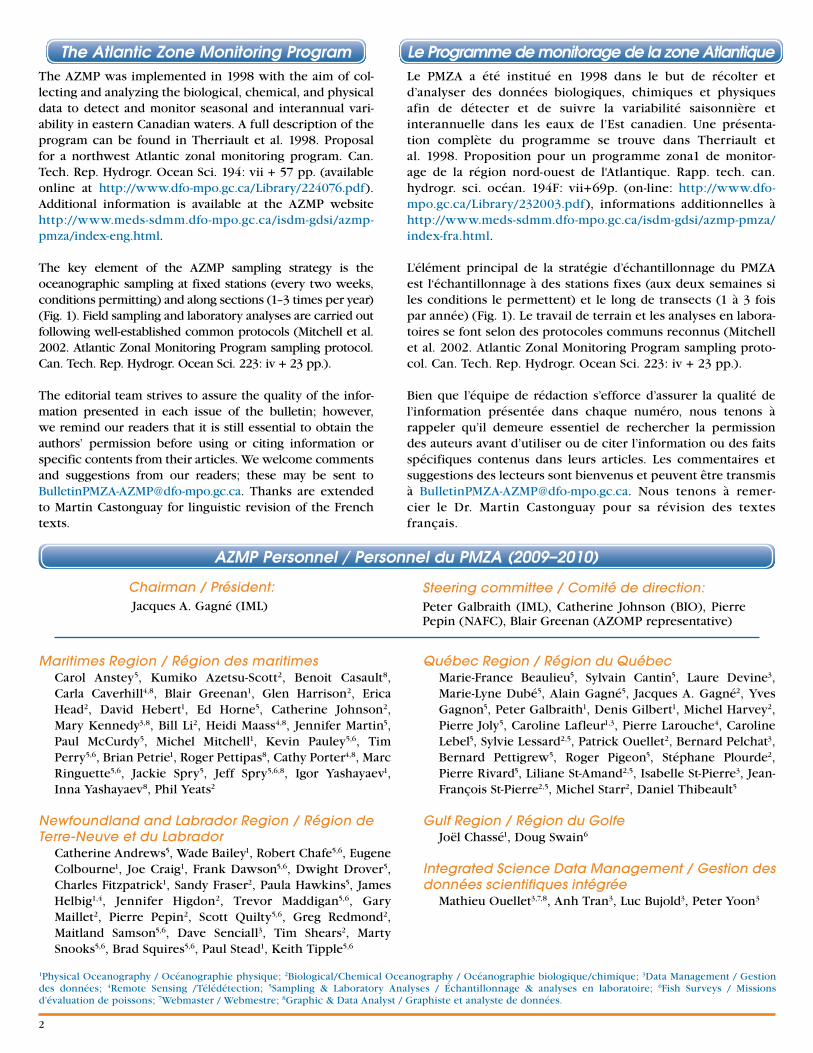
BulletinPMZA-AZMP@dfo-mpo.gc.caFig. 1 Locations of sections and fixed stations.

Localisation des transects et des stations fixes.

Le Bulletin du PMZA

The AZMP Bulletin

2010 No. 9

http://www.meds-sdmm.dfo-mpo.gc.ca/zmp/main_zmp_e.htmlISSN 1916-6362

2

The AZMP was implemented in 1998 with the aim of col-lecting and analyzing the biological, chemical, and physical data to detect and monitor seasonal and interannual vari-ability in eastern Canadian waters. A full description of the program can be found in Therriault et al. 1998. Proposal for a northwest Atlantic zonal monitoring program. Can. Tech. Rep. Hydrogr. Ocean Sci. 194: vii + 57 pp. (available online at http://www.dfo-mpo.gc.ca/Library/224076.pdf). Additional information is available at the AZMP website http://www.meds-sdmm.dfo-mpo.gc.ca/isdm-gdsi/azmp-pmza/index-eng.html.

The key element of the AZMP sampling strategy is the oceanographic sampling at fixed stations (every two weeks, conditions permitting) and along sections (1–3 times per year) (Fig. 1). Field sampling and laboratory analyses are carried out following well-established common protocols (Mitchell et al. 2002. Atlantic Zonal Monitoring Program sampling protocol. Can. Tech. Rep. Hydrogr. Ocean Sci. 223: iv + 23 pp.).

The editorial team strives to assure the quality of the infor-mation presented in each issue of the bulletin; however, we remind our readers that it is still essential to obtain the authors’ permission before using or citing information or specific contents from their articles. We welcome comments and suggestions from our readers; these may be sent to BulletinPMZA-AZMP@dfo-mpo.gc.ca. Thanks are extended to Martin Castonguay for linguistic revision of the French texts.

Le PMZA a été institué en 1998 dans le but de récolter et d’analyser des données biologiques, chimiques et physiques afin de détecter et de suivre la variabilité saisonnière et interannuelle dans les eaux de l’Est canadien. Une présenta-tion complète du programme se trouve dans Therriault et al. 1998. Proposition pour un programme zona1 de monitor-age de la région nord-ouest de l'Atlantique. Rapp. tech. can. hydrogr. sci. océan. 194F: vii+69p. (on-line: http://www.dfo-mpo.gc.ca/Library/232003.pdf), informations additionnelles à http://www.meds-sdmm.dfo-mpo.gc.ca/isdm-gdsi/azmp-pmza/index-fra.html.

L’élément principal de la stratégie d’échantillonnage du PMZA est l‘échantillonnage à des stations fixes (aux deux semaines si les conditions le permettent) et le long de transects (1 à 3 fois par année) (Fig. 1). Le travail de terrain et les analyses en labora-toires se font selon des protocoles communs reconnus (Mitchell et al. 2002. Atlantic Zonal Monitoring Program sampling proto-col. Can. Tech. Rep. Hydrogr. Ocean Sci. 223: iv + 23 pp.).

Bien que l’équipe de rédaction s’efforce d’assurer la qualité de l’information présentée dans chaque numéro, nous tenons à rappeler qu’il demeure essentiel de rechercher la permission des auteurs avant d’utiliser ou de citer l’information ou des faits spécifiques contenus dans leurs articles. Les commentaires et suggestions des lecteurs sont bienvenus et peuvent être transmis à BulletinPMZA-AZMP@dfo-mpo.gc.ca. Nous tenons à remer-cier le Dr. Martin Castonguay pour sa révision des textes français.

The Atlantic Zone Monitoring Program Le Programme de monitorage de la zone Atlantique

1Physical Oceanography / Océanographie physique; 2Biological/Chemical Oceanography / Océanographie biologique/chimique; 3Data Management / Gestion des données; 4Remote Sensing /Télédétection; 5Sampling & Laboratory Analyses / Échantillonnage & analyses en laboratoire; 6Fish Surveys / Missions d’évaluation de poissons; 7Webmaster / Webmestre; 8Graphic & Data Analyst / Graphiste et analyste de données.

Maritimes Region / Région des maritimes Carol Anstey5, Kumiko Azetsu-Scott2, Benoit Casault8,

Carla Caverhill4,8, Blair Greenan1, Glen Harrison2, Erica Head2, David Hebert1, Ed Horne5, Catherine Johnson2, Mary Kennedy3,8, Bill Li2, Heidi Maass4,8, Jennifer Martin5, Paul McCurdy5, Michel Mitchell1, Kevin Pauley5,6, Tim Perry5,6, Brian Petrie1, Roger Pettipas8, Cathy Porter4,8, Marc Ringuette5,6, Jackie Spry5, Jeff Spry5,6,8, Igor Yashayaev1, Inna Yashayaev8, Phil Yeats2

Newfoundland and Labrador Region / Région de Terre-Neuve et du Labrador Catherine Andrews5, Wade Bailey1, Robert Chafe5,6, Eugene

Colbourne1, Joe Craig1, Frank Dawson5,6, Dwight Drover5, Charles Fitzpatrick1, Sandy Fraser2, Paula Hawkins5, James Helbig1,4, Jennifer Higdon2, Trevor Maddigan5,6, Gary Maillet2, Pierre Pepin2, Scott Quilty5,6, Greg Redmond2, Maitland Samson5,6, Dave Senciall3, Tim Shears2, Marty Snooks5,6, Brad Squires5,6, Paul Stead1, Keith Tipple5,6

Québec Region / Région du Québec Marie-France Beaulieu5, Sylvain Cantin5, Laure Devine3,

Marie-Lyne Dubé5, Alain Gagné5, Jacques A. Gagné2, Yves Gagnon5, Peter Galbraith1, Denis Gilbert1, Michel Harvey2, Pierre Joly5, Caroline Lafleur1,3, Pierre Larouche4, Caroline Lebel5, Sylvie Lessard2,5, Patrick Ouellet2, Bernard Pelchat3, Bernard Pettigrew5, Roger Pigeon5, Stéphane Plourde2, Pierre Rivard5, Liliane St-Amand2,5, Isabelle St-Pierre3, Jean-François St-Pierre2,5, Michel Starr2, Daniel Thibeault5

Gulf Region / Région du Golfe Joël Chassé1, Doug Swain6

Integrated Science Data Management / Gestion des données scientifiques intégrée Mathieu Ouellet3,7,8, Anh Tran3, Luc Bujold3, Peter Yoon3

AZMP Personnel / Personnel du PMZA (2009–2010)

Chairman / Président: Jacques A. Gagné (IML)

Steering committee / Comité de direction:Peter Galbraith (IML), Catherine Johnson (BIO), Pierre Pepin (NAFC), Blair Greenan (AZOMP representative)

3

In 2010, the Atlantic Zone Monitoring Program (AZMP) cel-ebrates its 10th year of ocean observation—a very young age for an ocean monitoring program. The program is built upon sound international standards and operates with annual sup-port from DFO Science at the national and regional levels. Although the program represents the minimum effort to adequately detect and measure interannual variability over Atlantic Canada’s shelves and slopes, AZMP has grown into a strong, cooperative, coordinated, and coherent organization. Over the years, it has addressed specific issues such as the invasion of a Pacific phytoplankton species into the Gulf of St. Lawrence and the long-term changes in plankton over the Scotian Shelf – southern Newfoundland Shelf region revealed by the CPR program. By its contribution to the development of DFO's remote sensing capabilities, the program has pro-vided the foundation to relate phytoplankton abundance to recruitment success in Scotian Shelf haddock and northern shrimp. Its datasets were essential in describing the link between zooplankton and Atlantic mackerel recruitment. These achievements exemplify the growing zonal collabora-tion among AZMP scientists as well as the increased effort in data analysis. AZMP provides major contributions to various ecosystem overview and assessment reports. It is also the foundation for Canadian participation in current and planned international ocean observing and monitoring initiatives.

AZMP contributes to our understanding of profound changes in ecosystem dynamics from apex predators to nutrients. A quick survey shows that AZMP data form the basis of nearly 60 primary publications and peer-reviewed scientific reports produced by AZMP scientists since 2000; this total does not include the more than 140 research documents published for DFO, NAFO, and ICES, or the many abstracts and popular sci-ence papers. AZMP products are in demand: in 2008 alone—the only year for which statistics are available—about 6000 non-DFO people ranging from government agencies to NGOs to the private sector visited the AZMP website and proceeded beyond the home page. Close to 600 files of oceanographic data and over 1300 copies of various AZMP reports were downloaded, among which the bulletin was a favourite.

Although AZMP contributions are diverse, numerous, and often sought after, program sustainability is always a concern. We regularly explore how we can better apply new technolo-gies to improve information gathering while increasing effi-ciency in order to address our principal pressures: workload, ship availability, program cost, and emerging science issues like ocean acidification. We also recognize the need to be more responsive to regional requirements for science infor-mation and advice as we embark on the second decade of the program.

Le Programme de monitorage de la zone atlantique (PMZA) célèbre en 2010 son 10e anniversaire d'observation océanique, un âge bien jeune pour un tel programme. Il est réalisé selon de solides normes internationales avec l'appui des Sciences du MPO aux niveaux national et régionaux. Représentant le minimum nécessaire pour détecter et mesurer adéquate-ment la variabilité interannuelle sur les plateaux et pentes continentales du Canada atlantique, le PMZA constitue une équipe capable, coordonnée et cohérente. Au fil des ans, il a décrit des phénomènes importants comme l'intrusion d'une espèce de phytoplancton du Pacifique dans le golfe du Saint-Laurent ou les changements à long terme du plancton sur les plateaux Néo-Écossais et de Terre-Neuve grâce au programme Continuous Plankton Recorder. En contribuant au déve-loppement de la télédétection au MPO, il a permis de relier l'abondance du phytoplancton et le succès du recrutement chez l'aiglefin du plateau Néo-Écossais et la crevette nordique. Ses données ont servi à décrire le lien entre zooplancton et recrutement chez le maquereau bleu atlantique. Ces réalisa-tions témoignent de la collaboration croissante entre les sci-entifiques du PMZA et de l'effort déployé dans l'analyse des données. La contribution du PMZA est essentielle à la produc-tion de rapports et d'avis sur les écosystèmes marins. Il est le fer de lance de la participation canadienne aux programmes internationaux d'observation océanique.

Le PMZA contribue à améliorer notre compréhension de la dynamique des écosystèmes, des grands prédateurs aux nutri-ments. Un rapide inventaire montre que depuis 2000, les données du PMZA sont à l'origine de près de 60 publications primaires et rapports revus par les pairs produits par ses scientifiques. Et cela n'inclue pas plus de 140 documents de recherche publiés pour le MPO, l'OPANO et le CIEM, ni plusieurs résumés et documents de vulgarisation. Les produits du PMZA sont en demande. En 2008, seule année pour laquelle des statistiques sont disponibles, environ 6000 personnes externes au MPO, d'organismes gouver-nementaux canadiens et internationaux aux ONG et au secteur privé, ont visité le site Web du PMZA au-delà de sa page d'accueil. Elles ont téléchargé près de 600 fichiers de données et plus de 1300 rapports dont, en particulier, le Bulletin.

Malgré la qualité de ses produits, la pérennité du PMZA ne sera jamais assurée. Nous évaluons régulièrement les nou-velles technologies pour améliorer la collecte d'information, augmenter l'efficacité du programme et ainsi mieux faire face à nos principaux défis : charge de travail, disponibilité des navires, coûts du programme et nouveaux enjeux envi-ronnementaux comme l'acidification des océans. Alors que le jeune PMZA entreprend sa deuxième décennie, nous recon-naissons la nécessité de mieux répondre aux besoins régio-naux d'information et de conseils scientifiques.

AZMP: the first 10 yearsPMZA : les premières 10 années

Jacques A . Gagné (AZMP Chairman / Président PMZA) Institut Maurice-Lamontagne, C.P. 1000, Mont-Joli, QC, G5H 3Z4

jacques.gagne@dfo-mpo.gc.ca

4

Environmental Review Revue environnementale

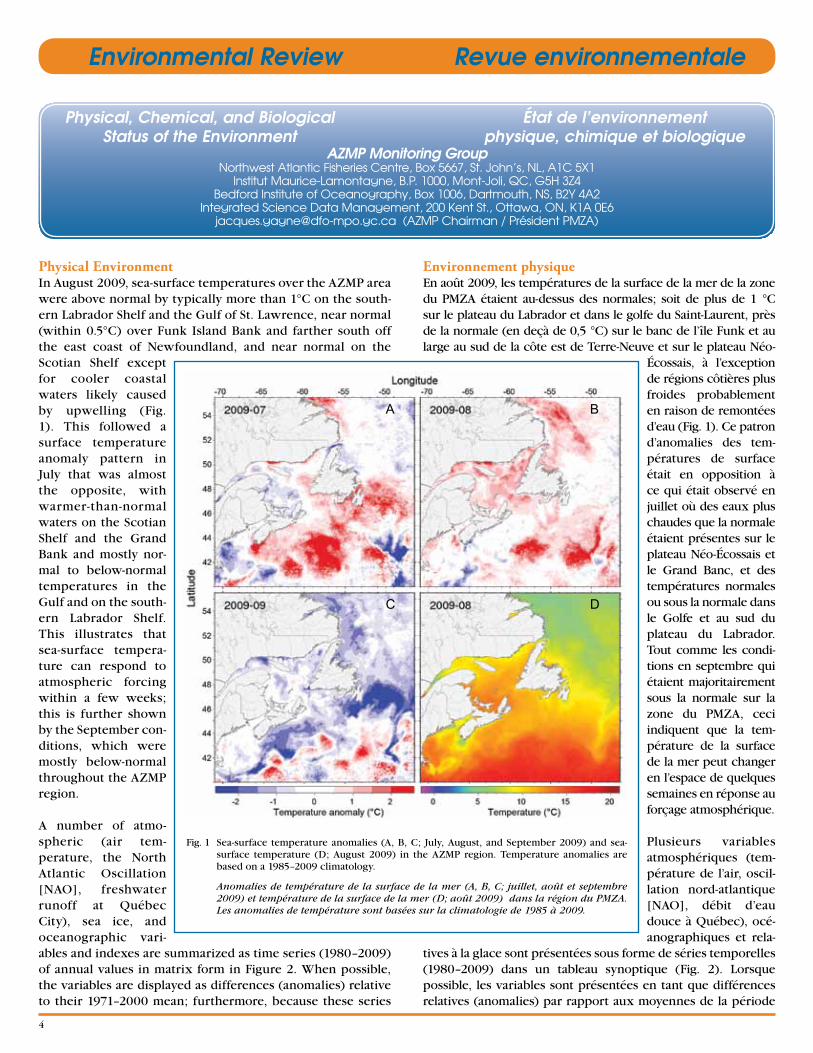
Physical EnvironmentIn August 2009, sea-surface temperatures over the AZMP area were above normal by typically more than 1°C on the south-ern Labrador Shelf and the Gulf of St. Lawrence, near normal (within 0.5°C) over Funk Island Bank and farther south off the east coast of Newfoundland, and near normal on the Scotian Shelf except for cooler coastal waters likely caused by upwelling (Fig. 1). This followed a surface temperature anomaly pattern in July that was almost the opposite, with warmer-than-normal waters on the Scotian Shelf and the Grand Bank and mostly nor-mal to below-normal temperatures in the Gulf and on the south-ern Labrador Shelf. This illustrates that sea-surface tempera-ture can respond to atmospheric forcing within a few weeks; this is further shown by the September con-ditions, which were mostly below-normal throughout the AZMP region.

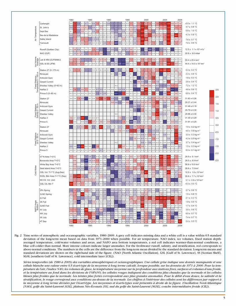
A number of atmo-spheric (air tem-perature, the North Atlantic Oscillation [NAO], freshwater runoff at Québec City), sea ice, and oceanographic vari-ables and indexes are summarized as time series (1980–2009) of annual values in matrix form in Figure 2. When possible, the variables are displayed as differences (anomalies) relative to their 1971–2000 mean; furthermore, because these series

Physical, Chemical, and Biological Status of the Environment

État de l’environnementphysique, chimique et biologique

AZMP Monitoring GroupNorthwest Atlantic Fisheries Centre, Box 5667, St. John’s, NL, A1C 5X1

Institut Maurice-Lamontagne, B.P. 1000, Mont-Joli, QC, G5H 3Z4Bedford Institute of Oceanography, Box 1006, Dartmouth, NS, B2Y 4A2

Integrated Science Data Management, 200 Kent St., Ottawa, ON, K1A 0E6jacques.gagne@dfo-mpo.gc.ca (AZMP Chairman / Président PMZA)

Environnement physiqueEn août 2009, les températures de la surface de la mer de la zone du PMZA étaient au-dessus des normales; soit de plus de 1 °C sur le plateau du Labrador et dans le golfe du Saint-Laurent, près de la normale (en deçà de 0,5 °C) sur le banc de l’île Funk et au large au sud de la côte est de Terre-Neuve et sur le plateau Néo-

Écossais, à l’exception de régions côtières plus froides probablement en raison de remontées d’eau (Fig. 1). Ce patron d’anomalies des tem-pératures de surface était en opposition à ce qui était observé en juillet où des eaux plus chaudes que la normale étaient présentes sur le plateau Néo-Écossais et le Grand Banc, et des températures normales ou sous la normale dans le Golfe et au sud du plateau du Labrador. Tout comme les condi-tions en septembre qui étaient majoritairement sous la normale sur la zone du PMZA, ceci indiquent que la tem-pérature de la surface de la mer peut changer en l’espace de quelques semaines en réponse au forçage atmosphérique.

Plusieurs variables atmosphériques (tem-pérature de l’air, oscil-lation nord-atlantique [NAO], débit d’eau douce à Québec), océ-anographiques et rela-

tives à la glace sont présentées sous forme de séries temporelles (1980–2009) dans un tableau synoptique (Fig. 2). Lorsque possible, les variables sont présentées en tant que différences relatives (anomalies) par rapport aux moyennes de la période

Fig. 1 Sea-surface temperature anomalies (A, B, C; July, August, and September 2009) and sea-surface temperature (D; August 2009) in the AZMP region. Temperature anomalies are based on a 1985–2009 climatology.

Anomalies de température de la surface de la mer (A, B, C; juillet, août et septembre 2009) et température de la surface de la mer (D; août 2009) dans la région du PMZA. Les anomalies de température sont basées sur la climatologie de 1985 à 2009.

A B

DC

5

Fig. 2 Time series of atmospheric and oceanographic variables, 1980–2009. A grey cell indicates missing data and a white cell is a value within 0.5 standard deviation of the long-term mean based on data from 1971–2000 when possible. For air temperature, NAO index, ice volumes, fixed station depth-averaged temperature, cold-water volumes and areas, and NAFO area bottom temperatures, a red cell indicates warmer-than-normal conditions, a blue cell colder than normal. More intense colours indicate larger anomalies. For the freshwater runoff, salinity, and stratification, red corresponds to above-normal conditions. The numbers in the cells are the difference from the long-term mean divided by the standard deviation. Long-term means and standard deviations are shown on the right-hand side of the figure. (NAO [North Atlantic Oscillation], GSL [Gulf of St. Lawrence], SS [Scotian Shelf], SGSL [southern Gulf of St. Lawrence], cold intermediate layer [CIL]).

Séries temporelles (de 1980 à 2009) des variables atmosphériques et océanographiques. Une cellule grise indique une donnée manquante et une cellule blanche une valeur entre 0,5 écart-type de la moyenne à long terme calculé, lorsque possible, sur les données de 1971 à 2000. Pour la tem-pérature de l’air, l’indice NAO, les volumes de glace, la température moyenne sur la profondeur aux stations fixes, surfaces et volumes d’eau froide, et la température au fond dans les divisions de l’OPANO, les cellules rouges indiquent des conditions plus chaudes que la normale et les cellules bleues plus froides que la normale. Les teintes plus fortes correspondent aux plus grandes anomalies. Pour le débit d’eau douce, la salinité et la stratification, le rouge correspond aux conditions au-dessus de la normale. Les chiffres à l’intérieur des cellules sont les différences par rapport à la moyenne à long terme divisées par l’écart-type. Les moyennes et écarts-types sont présentés à droite de la figure. (Oscillation Nord-Atlantique [NAO], golfe du Saint-Laurent [GSL], plateau Néo-Écossais [SS], sud du golfe du Saint-Laurent [SGSL], couche intermédiaire froide [CIL]).

0

0.1

0.2

0.3

0.4

0.5

0.6

0.7

0.8

0.9

1

Cartwright

St. John’s

Sept-Îles

Îles-de-la Madeleine

Sable Island

Yarmouth

Air

Tem

pera

ture

Runoff (Québec City)

NAO (DJF) Lab & Nfld (DJFMAMJ)

GSL & SS (JFM)

Ice

Vol

ume

Ave

rage

Station 27 (0−175 m)

Rimouski

Anticosti Gyre

Gaspé Current

Shediac Valley (0−83 m)

Halifax 2

Prince 5 (0−90 m)

Fixe

d S

tatio

nsTe

mpe

ratu

re 0

- 10

0 m

Station 27

Rimouski

Anticosti Gyre

Gaspé Current

Shediac Valley

Halifax 2

Prince 5

Fixe

d S

tatio

nsS

alin

ity 0

- 50

m

Station 27

Rimouski

Anticosti Gyre

Gaspé Current

Shediac Valley

Halifax 2

Prince 5

Fixe

d S

tatio

ns∆σ

0 -

50 m

47°N Area T<0°C

Bonavista Area T<0°C

White Bay Area T<0°C

Seal Island Area T<0°C

GSL Vol. T<1°C (Aug-Sep)

SGSL Btm Area T<1°C (Sep)

SS CIL Vol. (Jul)

GSL CIL Min T

Col

d W

ater

3Ps Spring

3LNO Spring

2J Fall

3K Fall

3LNO Fall

4V July

4W July

4X July

4T Sep

NA

FO A

reas

Bot

tom

T

0.4 1.8 -1.0 -0.1 -0.7 -0.2 -0.6 1.0 0.1 -0.2 -0.9 -1.3 -1.1 -1.0 -0.2 0.2 1.1 0.1 1.2 1.8 1.1 1.2 0.2 1.0 1.8 1.6 2.6 0.6 0.7 1.0 -0.5 ± 1.1 °C

-0.8 1.5 -0.6 1.0 0.7 -1.3 -0.6 -0.1 0.7 -0.2 -0.1 -1.0 -1.4 -1.1 -0.0 -0.3 0.8 -0.7 1.1 2.5 1.6 0.8 0.1 0.9 1.1 1.3 2.2 0.4 1.4 1.4 4.7 ± 0.8 °C

0.1 1.8 -1.1 0.5 0.0 -0.1 -0.8 1.0 0.2 -0.5 -0.5 -0.6 -1.1 -0.9 -0.6 0.2 0.9 -0.6 1.6 2.2 0.5 1.4 -1.5 -0.3 -0.2 -0.0 1.7 -0.5 0.1 0.6 0.9 ± 1.0 °C

-0.9 1.1 -0.8 -0.4 0.3 0.3 0.3 -0.1 0.1 0.1 -0.9 -1.3 0.0 0.3 0.9 -0.3 1.7 2.7 1.4 1.7 0.5 0.7 0.7 1.4 3.1 0.9 2.0 1.3 4.3 ± 0.8 °C

-1.1 1.4 -0.3 1.3 1.3 -1.5 -1.0 -0.6 -0.2 -0.5 0.1 0.1 -0.8 0.0 0.8 -0.2 -0.1 -0.9 1.3 2.8 2.0 0.7 0.3 0.2 -0.3 1.0 2.1 -0.2 0.7 0.7 7.6 ± 0.7 °C-1.0 0.7 -0.3 0.9 1.1 -0.6 -0.3 -0.3 -0.1 -0.8 1.4 0.6 -2.0 -0.8 0.3 0.2 -0.3 -0.8 1.1 2.7 0.9 0.7 1.0 -0.1 -1.2 0.6 2.3 -0.3 1.2 0.7 7.0 ± 0.6 °C

-0.2 0.6 -0.6 0.4 0.4 0.2 1.2 -0.6 -1.1 -1.9 -0.7 -0.6 -1.0 0.1 -0.5 -0.7 0.6 0.5 0.4 -1.5 -1.0 -2.0 -1.4 -1.6 -1.1 -0.6 -0.0 -1.5 -0.0 -0.3

-0.4 0.5 -0.7 0.7 1.2 -1.3 -1.1 -1.0 -0.6 1.6 1.1 0.3 0.2 0.9 0.4 1.3 -1.4 -0.6 -0.3 1.2 1.1 -1.0 -0.4 -0.4 -1.1 0.5 -0.4 0.3 0.5 0.1 20.8 ± 8.6 mbar

-0.9 -1.4 -0.8 1.1 1.5 1.4 -0.9 -0.3 -0.7 -0.8 0.4 1.7 1.0 1.6 1.8 0.4 -1.2 -0.4 -0.4 -1.0 -0.8 -1.0 -0.8 -0.1 -1.3 -1.1 -1.5 -0.4 -0.3 0.3 55.4 ± 25.4 km3

-1.3 -1.4 -0.8 -1.4 -0.4 0.1 -0.0 0.1 -0.0 0.1 1.3 0.6 0.6 2.0 2.1 0.6 -0.3 0.0 -1.6 -1.2 -1.9 -1.4 -1.6 1.0 -1.3 -0.6 -2.4 -1.8 -0.9 -0.3 44.4 ± 14.5 x 103 km3

-0.1 1.3 1.5 0.3 -1.1 -1.1 0.3 -0.1 -0.1 0.4 -0.1 -2.5 -0.7 -1.0 0.2 -0.4 2.5 -0.1 -0.1 1.2 1.1 1.3 0.7 1.2 3.0 2.0 3.3 0.0 0.8 0.4 0.3 ± 0.3 °C

-0.1 -1.0 -0.2 -2.0 -0.1 0.1 -1.8 0.1 1.4 0.9 1.5 1.3 -0.0 -1.5 0.2 0.7 0.0 -0.0 0.8 2.3 ± 0.6 °C

-0.1 0.1 -1.9 -1.3 0.6 1.3 1.8 -0.1 -0.8 0.0 0.2 0.2 1.8 ± 0.3 °C

0.2 -1.7 0.6 -0.5 -1.0 0.0 1.3 -1.0 -0.1 1.7 -0.5 0.9 2.6 ± 0.4 °C

0.3 -1.4 0.6 0.6 0.6 -0.3 -0.7 -1.3 -1.4 -0.6 1.0 1.3 -0.4 7.2 ± 1.2 °C

0.3 1.4 -1.1 0.6 1.1 0.3 0.5 -0.7 -0.9 0.5 0.4 -0.0 0.2 -0.6 -0.8 0.3 -0.2 -1.6 -1.8 0.6 2.0 -0.3 0.4 -1.0 -0.9 0.1 1.5 -2.1 -1.6 0.1 4.6 ± 0.6 °C

-0.3 -0.3 0.0 -0.0 0.2 -0.0 0.3 -1.2 -0.7 -0.6 -0.1 0.2 -2.2 -1.8 1.7 0.4 -0.3 -0.3 0.1 1.9 1.9 0.1 1.9 -0.3 -1.7 -0.6 2.9 0.2 0.8 0.4 6.8 ± 0.4 °C

0.4 0.4 1.4 -0.6 -1.5 -0.1 0.4 1.0 1.8 1.0 1.8 -0.9 -1.3 -0.4 -1.1 -1.7 -0.1 0.3 0.3 -0.4 0.4 -0.9 1.1 0.5 0.9 1.0 0.9 1.0 1.5 0.3 31.63 ± 0.26

0.8 -0.6 -1.2 -0.1 0.6 -1.6 -1.0 -0.5 0.9 0.7 0.8 1.5 1.6 -0.2 -0.6 0.2 1.1 -1.0 -1.4 29.21 ± 0.44

-1.5 -0.8 -1.2 0.9 0.3 0.3 1.4 1.4 -1.1 -0.1 -0.4 0.8 31.46 ± 0.19

0.3 -1.5 -1.8 1.3 0.0 0.3 0.3 1.6 -0.2 -0.4 -0.5 0.7 29.79 ± 0.30

0.0 0.0 0.0 0.3 1.1 2.1 -0.8 -0.6 -0.1 1.0 -1.7 -0.1 29.96 ± 0.30

0.6 0.1 -0.6 2.6 -1.6 -0.3 -0.2 -0.1 1.0 -1.1 -0.5 -0.7 -2.0 -1.5 0.1 0.4 0.6 -0.1 1.5 0.3 0.1 -0.3 -0.0 0.0 -0.2 31.30 ± 0.29

1.8 -0.4 -0.5 -1.0 1.5 0.7 0.1 0.6 0.1 0.8 -1.0 -1.2 -1.1 1.0 -0.3 -2.0 -0.6 -1.4 0.3 0.4 0.2 1.3 0.6 0.1 -1.7 -0.1 0.8 -0.8 -0.0 31.91 ± 0.25

-1.8 0.2 -0.8 0.9 1.8 -0.4 -1.2 0.4 2.1 0.1 -0.9 0.1 -0.1 -0.8 -0.1 1.6 -1.1 0.6 1.2 1.4 0.7 1.4 -0.2 0.0 -0.3 0.3 1.4 0.7 1.1 0.0 1.0 ± 0.2 kg m-3

-1.2 0.4 0.8 0.5 -0.7 1.6 1.5 -0.7 -1.8 0.1 -1.3 -0.6 -0.9 0.3 -0.1 0.2 0.1 1.8 0.3 4.5 ± 0.6 kg m-3

1.0 -0.0 -0.3 -0.8 -0.3 1.2 -0.6 -0.4 -0.9 -0.3 2.3 -1.0 3.0 ± 0.3 kg m-3

-1.1 1.0 -0.4 -0.7 0.3 -0.4 1.2 0.3 -1.0 1.9 -1.0 4.3 ± 0.5 kg m-3

-0.2 -0.6 0.1 -0.8 -0.5 -0.2 -0.1 0.4 0.4 -0.9 3.0 0.2 3.7 ± 0.4 kg m-3

-0.9 0.0 -2.0 2.3 -0.0 0.0 -1.8 1.4 1.6 0.7 0.1 -0.0 0.3 1.2 0.6 0.1 0.2 -0.0 -0.4 -0.4 -1.2 0.4 -0.0 0.5 -0.7 1.5 ± 0.3 kg m-3

0.0 0.1 0.4 -0.3 0.3 0.4 0.6 0.4 -0.7 -0.1 -0.2 -0.3 -0.2 -0.1 0.3 0.5 0.0 -0.2 -0.3 -0.0 -0.3 -0.3 -0.5 -0.3 -0.3 -0.5 0.0 -0.3 -0.0 -0.2 0.3 ± 0.1 kg m-3

-1.1 -0.9 1.4 0.8 1.1 -0.5 0.3 0.8 -0.0 1.7 0.6 1.3 -0.0 0.3 -0.8 0.3 -0.7 -1.4 -1.3 -0.5 -0.8 -0.4 -2.7 -1.1 -2.7 -0.2 -1.0 -0.2 28.5 ± 5.1 km2

-0.6 1.0 2.4 0.9 -0.9 -1.0 0.1 0.0 1.7 1.8 -0.0 0.5 -0.0 -1.0 -0.5 -1.0 -0.3 -0.9 -0.2 -1.2 -1.0 -0.6 -1.7 -1.4 -1.7 -1.0 -1.4 -0.4 28.5 ± 8.9 km2

-0.9 0.1 1.3 0.2 -0.5 -0.8 0.3 0.8 1.7 0.9 1.0 0.8 1.0 -0.7 -0.1 -0.5 -1.0 -1.1 0.1 -0.6 -1.0 -0.5 -1.9 -1.3 -1.8 -1.1 -0.6 0.3 58.8 ± 15.0 km2

-0.3 -0.5 0.6 0.8 1.5 0.7 -1.0 0.5 -0.5 1.3 1.4 0.5 0.7 0.6 -1.2 -0.5 -1.5 -0.6 -1.9 0.3 -0.5 -1.1 -0.4 -1.4 -1.1 -0.6 -0.8 0.0 0.6 28.8 ± 7.9 km2

-0.6 0.0 0.7 -0.5 0.2 -0.1 1.6 1.5 0.7 0.5 1.3 1.0 0.1 0.4 -1.3 -2.1 0.3 -0.9 1.0 -0.1 -1.0 -2.1 -0.0 0.7 -0.6 10.0 ± 1.8 x 103 km3

-0.9 -1.6 -2.6 -1.2 1.2 0.2 0.1 -0.2 -1.0 0.9 0.6 0.6 1.5 0.5 0.7 1.4 0.7 0.6 1.1 -0.6 -1.0 0.1 -0.8 0.4 -0.1 -0.7 -1.1 -0.4 0.7 -1.0 35.6 ± 7.7 x 103 km2

-0.8 -1.0 -1.1 -0.8 -0.8 -0.6 -0.5 0.0 0.8 1.5 1.3 1.1 0.8 0.9 1.0 1.4 2.3 -0.1 -1.8 2.1 0.2 1.9 3.2 -0.1 -1.1 1.9 1.6 -0.1 5.1 ± 0.9 x 103 km3

3.3 1.3 0.9 1.1 -0.0 0.1 -1.0 -0.8 -0.3 -0.6 -1.0 -1.1 -1.0 -0.8 -1.0 -0.9 -0.6 -0.4 -0.8 0.2 0.8 0.2 0.2 -0.9 0.1 0.5 1.0 0.2 -0.7 -0.2 -0.3 ± 0.5 °C

-1.5 1.2 -1.2 -0.3 1.3 -0.7 0.1 -0.9 -0.4 -0.8 -1.6 -0.9 -0.9 -0.6 -0.4 -0.9 -0.0 -0.6 -0.3 0.5 0.7 -0.7 -0.2 -1.3 -0.3 0.4 -1.0 -0.9 -0.2 2.7 ± 0.6 °C

0.5 1.4 -0.0 2.1 0.2 -0.1 -1.0 -0.5 -0.2 -0.8 -1.7 -1.5 -1.1 -0.7 -0.7 -0.7 -0.2 -0.5 0.2 0.6 0.6 0.1 0.0 -0.5 1.0 0.4 0.4 0.4 0.4 1.5 ± 0.8 °C

-0.2 1.1 -1.1 -1.2 -0.9 -0.6 0.0 -1.4 0.0 -0.9 -0.4 -0.0 -1.1 -0.6 -0.5 -0.4 1.4 0.7 1.1 1.9 1.3 1.7 1.4 2.3 2.6 2.5 1.5 2.4 1.3 1.5 2.1 ± 0.3 °C

0.4 0.6 -2.3 -0.1 0.2 -1.4 0.9 -0.3 0.2 0.3 -0.7 -0.3 -1.5 -1.3 -0.8 0.4 0.5 1.2 0.8 2.0 0.6 0.9 1.1 1.4 1.9 1.8 0.9 2.6 1.3 1.4 1.9 ± 0.5 °C

-0.5 -0.2 -1.4 -1.8 -1.7 -0.1 -0.0 0.2 0.4 2.1 -0.1 0.1 -0.0 0.1 0.9 1.8 0.1 0.1 -0.1 0.0 1.7 ± 0.4 °C

1.2 1.2 -1.2 -0.3 2.5 -0.3 0.4 -1.3 0.8 -1.1 -1.6 -1.6 -0.5 -0.4 -1.0 -0.6 -1.1 -0.3 -0.3 0.6 0.9 -0.3 0.3 -1.4 -1.3 0.4 0.9 -0.6 -0.2 0.2 3.6 ± 0.6 °C

0.8 0.6 -1.3 -0.3 1.7 1.6 1.2 -1.0 -1.1 -0.7 -0.8 -1.2 -0.5 0.3 0.2 0.1 -0.6 -0.5 -2.4 0.3 1.3 -1.2 0.2 -1.3 -2.9 -0.4 1.3 -1.4 -1.8 0.1 6.5 ± 0.7 °C

0.4 -0.7 0.1 0.0 0.8 1.6 0.6 -1.6 -0.4 -0.2 -0.3 -1.0 0.1 -0.5 1.1 -0.9 -0.6 0.1 -2.7 0.8 1.3 -1.5 1.1 0.1 -1.9 -0.1 1.1 -1.6 -0.7 -0.2 7.4 ± 0.7 °C

1.5 2.2 1.1 0.6 -1.9 0.8 0.9 -0.2 -0.1 -0.3 -0.9 0.6 -2.0 -0.1 -0.4 -0.8 -0.3 -0.9 -0.5 1.0 1.2 0.1 1.6 0.4 0.6 0.1 1.1 1.5 -0.1 2.1 2.4 ± 0.5 °C

12.5 ± 1.1 x 103 m3s-1

1980 1985 1990 1995 2000 2005 2009

1980 1985 1990 1995 2000 2005 2009

2.5

2.0

1.5

1.0

0.5

0.0

-0.5

-1.0

-1.5

-2.0

-2.5

6

have different units (e.g., °C, m3, m2), each anomaly time series is normalized by dividing by its standard deviation (SD), which is also based on the 1971–2000 period. This allows a more direct comparison of the series. Missing data are represented by grey cells, values within 0.5 SD of the aver-age as white cells (these are considered to represent normal conditions), and conditions corresponding to warmer than normal (higher temperatures, reduced ice volumes, reduced cold-water volumes or areas, negative NAO index) by more than 0.5 SD as red cells, with more intense reds correspond-ing to increasingly warmer conditions. Similarly, blue rep-resents colder-than-normal conditions. Higher-than-normal freshwater inflow and stratification anomalies are shown as red but are not necessarily indicative of warmer-than-normal conditions.

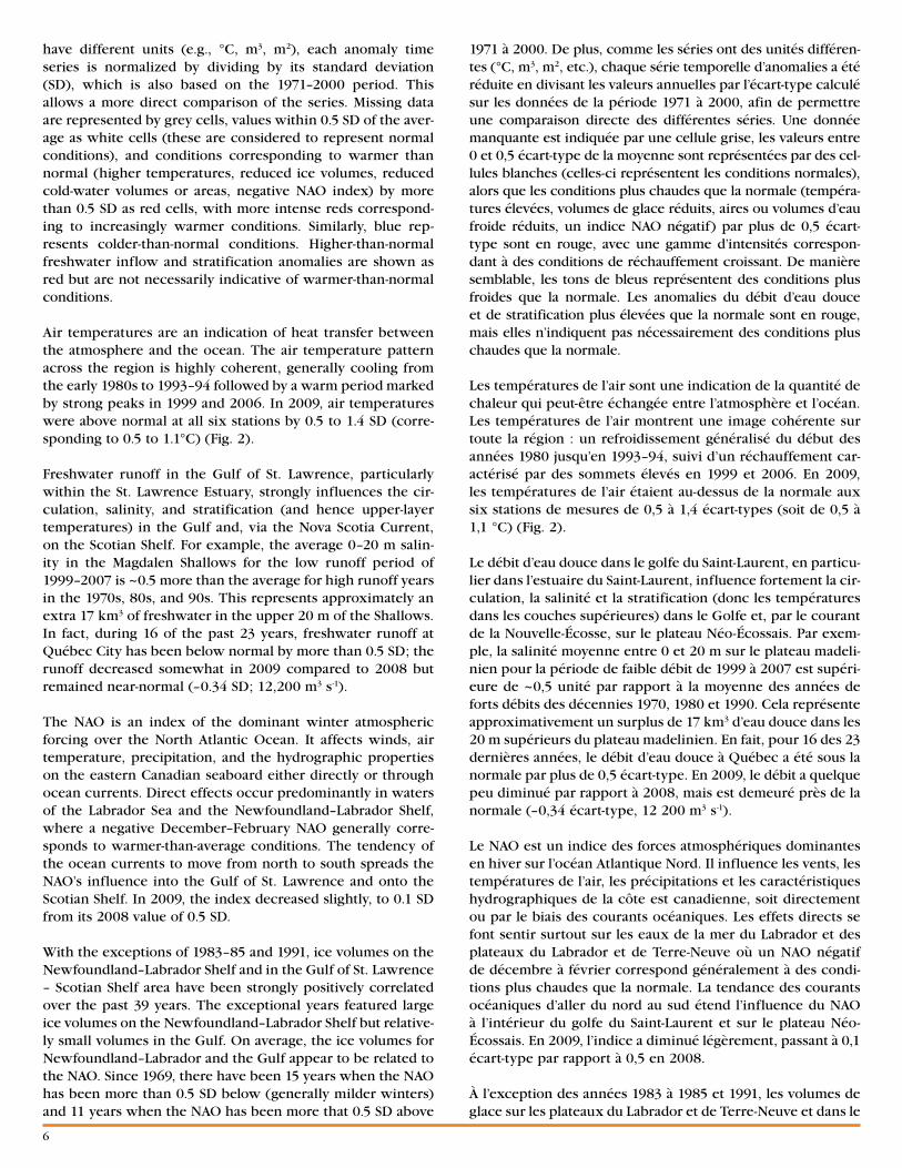
Air temperatures are an indication of heat transfer between the atmosphere and the ocean. The air temperature pattern across the region is highly coherent, generally cooling from the early 1980s to 1993–94 followed by a warm period marked by strong peaks in 1999 and 2006. In 2009, air temperatures were above normal at all six stations by 0.5 to 1.4 SD (corre-sponding to 0.5 to 1.1°C) (Fig. 2).

Freshwater runoff in the Gulf of St. Lawrence, particularly within the St. Lawrence Estuary, strongly influences the cir-culation, salinity, and stratification (and hence upper-layer temperatures) in the Gulf and, via the Nova Scotia Current, on the Scotian Shelf. For example, the average 0–20 m salin-ity in the Magdalen Shallows for the low runoff period of 1999–2007 is ~0.5 more than the average for high runoff years in the 1970s, 80s, and 90s. This represents approximately an extra 17 km3 of freshwater in the upper 20 m of the Shallows. In fact, during 16 of the past 23 years, freshwater runoff at Québec City has been below normal by more than 0.5 SD; the runoff decreased somewhat in 2009 compared to 2008 but remained near-normal (–0.34 SD; 12,200 m3 s-1).

The NAO is an index of the dominant winter atmospheric forcing over the North Atlantic Ocean. It affects winds, air temperature, precipitation, and the hydrographic properties on the eastern Canadian seaboard either directly or through ocean currents. Direct effects occur predominantly in waters of the Labrador Sea and the Newfoundland–Labrador Shelf, where a negative December–February NAO generally corre-sponds to warmer-than-average conditions. The tendency of the ocean currents to move from north to south spreads the NAO’s influence into the Gulf of St. Lawrence and onto the Scotian Shelf. In 2009, the index decreased slightly, to 0.1 SD from its 2008 value of 0.5 SD.

With the exceptions of 1983–85 and 1991, ice volumes on the Newfoundland–Labrador Shelf and in the Gulf of St. Lawrence – Scotian Shelf area have been strongly positively correlated over the past 39 years. The exceptional years featured large ice volumes on the Newfoundland–Labrador Shelf but relative-ly small volumes in the Gulf. On average, the ice volumes for Newfoundland–Labrador and the Gulf appear to be related to the NAO. Since 1969, there have been 15 years when the NAO has been more than 0.5 SD below (generally milder winters) and 11 years when the NAO has been more that 0.5 SD above

1971 à 2000. De plus, comme les séries ont des unités différen-tes (°C, m3, m2, etc.), chaque série temporelle d’anomalies a été réduite en divisant les valeurs annuelles par l’écart-type calculé sur les données de la période 1971 à 2000, afin de permettre une comparaison directe des différentes séries. Une donnée manquante est indiquée par une cellule grise, les valeurs entre 0 et 0,5 écart-type de la moyenne sont représentées par des cel-lules blanches (celles-ci représentent les conditions normales), alors que les conditions plus chaudes que la normale (tempéra-tures élevées, volumes de glace réduits, aires ou volumes d’eau froide réduits, un indice NAO négatif) par plus de 0,5 écart-type sont en rouge, avec une gamme d’intensités correspon-dant à des conditions de réchauffement croissant. De manière semblable, les tons de bleus représentent des conditions plus froides que la normale. Les anomalies du débit d’eau douce et de stratification plus élevées que la normale sont en rouge, mais elles n’indiquent pas nécessairement des conditions plus chaudes que la normale.

Les températures de l’air sont une indication de la quantité de chaleur qui peut-être échangée entre l’atmosphère et l’océan. Les températures de l’air montrent une image cohérente sur toute la région : un refroidissement généralisé du début des années 1980 jusqu’en 1993–94, suivi d’un réchauffement car-actérisé par des sommets élevés en 1999 et 2006. En 2009, les températures de l’air étaient au-dessus de la normale aux six stations de mesures de 0,5 à 1,4 écart-types (soit de 0,5 à 1,1 °C) (Fig. 2).

Le débit d’eau douce dans le golfe du Saint-Laurent, en particu-lier dans l’estuaire du Saint-Laurent, influence fortement la cir-culation, la salinité et la stratification (donc les températures dans les couches supérieures) dans le Golfe et, par le courant de la Nouvelle-Écosse, sur le plateau Néo-Écossais. Par exem-ple, la salinité moyenne entre 0 et 20 m sur le plateau madeli-nien pour la période de faible débit de 1999 à 2007 est supéri-eure de ~0,5 unité par rapport à la moyenne des années de forts débits des décennies 1970, 1980 et 1990. Cela représente approximativement un surplus de 17 km3 d’eau douce dans les 20 m supérieurs du plateau madelinien. En fait, pour 16 des 23 dernières années, le débit d’eau douce à Québec a été sous la normale par plus de 0,5 écart-type. En 2009, le débit a quelque peu diminué par rapport à 2008, mais est demeuré près de la normale (–0,34 écart-type, 12 200 m3 s-1).

Le NAO est un indice des forces atmosphériques dominantes en hiver sur l’océan Atlantique Nord. Il influence les vents, les températures de l’air, les précipitations et les caractéristiques hydrographiques de la côte est canadienne, soit directement ou par le biais des courants océaniques. Les effets directs se font sentir surtout sur les eaux de la mer du Labrador et des plateaux du Labrador et de Terre-Neuve où un NAO négatif de décembre à février correspond généralement à des condi-tions plus chaudes que la normale. La tendance des courants océaniques d’aller du nord au sud étend l’influence du NAO à l’intérieur du golfe du Saint-Laurent et sur le plateau Néo-Écossais. En 2009, l’indice a diminué légèrement, passant à 0,1 écart-type par rapport à 0,5 en 2008.

À l’exception des années 1983 à 1985 et 1991, les volumes de glace sur les plateaux du Labrador et de Terre-Neuve et dans le

7

(generally colder winters) normal. The difference in the ice volumes between these two groups of years (colder vs. milder) is 5 km3 for the Gulf of St. Lawrence – Scotian Shelf (monthly average for Jan.–Mar.) and 24 km3 for the Newfoundland–Labrador Shelf (monthly average for Dec.–June). For the past decade, ice volumes on the Newfoundland–Labrador Shelf and the Gulf of St. Lawrence – Scotian Shelf have generally been lower than normal. However, the ice volumes in 2009 were within 0.5 SD of normal for the Gulf of St. Lawrence and Scotian Shelf as well as for the Newfoundland–Labrador region over the entire AZMP area.

There are sufficient data to estimate annual 0–100 m (or 0–bottom if the depth is <100 m) temperature anomalies for Station 27, Prince 5, and Halifax 2; however, the four series from the Gulf have sufficient data to estimate May to October anomalies for only 35%–60% of the years since 1980. In 2009, temperatures at Station 27, Shediac, Anticosti Gyre, Halifax 2, and Prince 5 were within 0.5 SD of normal, whereas the temperature was above normal at Rimouski sta-tion (by 0.8 SD) and Gaspé Current (by 0.9 SD).

The annual 0–50 m salinity anomalies were within 0.5 SD of normal at the three stations located outside of the Gulf (Station 27, Prince 5, and Halifax 2). Within the Gulf, anoma-lies were calculated from May to October and were negative (by 1.4 SD) at Rimouski station, positive at Anticosti Gyre and Gaspé Current (by 0.8 and 0.7 SD respectively), and within 0.5 SD of normal at Shediac Valley. The annual 0–50 m strati-fication index was near normal at Station 27, Rimouski sta-tion, and Shediac Valley, and below normal at Anticosti Gyre, Gaspé Current, Halifax 2, and near Prince 5 (the first two by –1.0 SD and the last two by –0.7 SD).

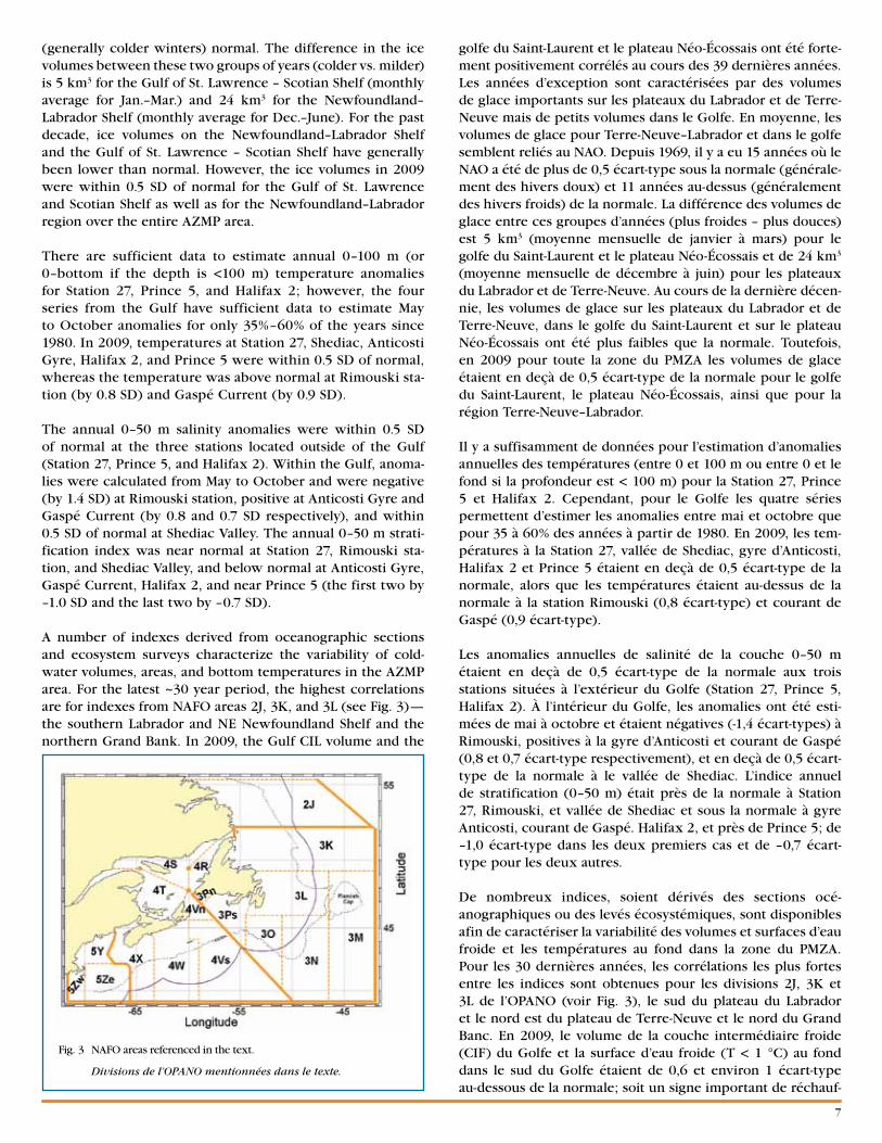
A number of indexes derived from oceanographic sections and ecosystem surveys characterize the variability of cold-water volumes, areas, and bottom temperatures in the AZMP area. For the latest ~30 year period, the highest correlations are for indexes from NAFO areas 2J, 3K, and 3L (see Fig. 3)—the southern Labrador and NE Newfoundland Shelf and the northern Grand Bank. In 2009, the Gulf CIL volume and the

golfe du Saint-Laurent et le plateau Néo-Écossais ont été forte-ment positivement corrélés au cours des 39 dernières années. Les années d’exception sont caractérisées par des volumes de glace importants sur les plateaux du Labrador et de Terre-Neuve mais de petits volumes dans le Golfe. En moyenne, les volumes de glace pour Terre-Neuve–Labrador et dans le golfe semblent reliés au NAO. Depuis 1969, il y a eu 15 années où le NAO a été de plus de 0,5 écart-type sous la normale (générale-ment des hivers doux) et 11 années au-dessus (généralement des hivers froids) de la normale. La différence des volumes de glace entre ces groupes d’années (plus froides – plus douces) est 5 km3 (moyenne mensuelle de janvier à mars) pour le golfe du Saint-Laurent et le plateau Néo-Écossais et de 24 km3 (moyenne mensuelle de décembre à juin) pour les plateaux du Labrador et de Terre-Neuve. Au cours de la dernière décen-nie, les volumes de glace sur les plateaux du Labrador et de Terre-Neuve, dans le golfe du Saint-Laurent et sur le plateau Néo-Écossais ont été plus faibles que la normale. Toutefois, en 2009 pour toute la zone du PMZA les volumes de glace étaient en deçà de 0,5 écart-type de la normale pour le golfe du Saint-Laurent, le plateau Néo-Écossais, ainsi que pour la région Terre-Neuve–Labrador.

Il y a suffisamment de données pour l’estimation d’anomalies annuelles des températures (entre 0 et 100 m ou entre 0 et le fond si la profondeur est < 100 m) pour la Station 27, Prince 5 et Halifax 2. Cependant, pour le Golfe les quatre séries permettent d’estimer les anomalies entre mai et octobre que pour 35 à 60% des années à partir de 1980. En 2009, les tem-pératures à la Station 27, vallée de Shediac, gyre d’Anticosti, Halifax 2 et Prince 5 étaient en deçà de 0,5 écart-type de la normale, alors que les températures étaient au-dessus de la normale à la station Rimouski (0,8 écart-type) et courant de Gaspé (0,9 écart-type).

Les anomalies annuelles de salinité de la couche 0–50 m étaient en deçà de 0,5 écart-type de la normale aux trois stations situées à l’extérieur du Golfe (Station 27, Prince 5, Halifax 2). À l’intérieur du Golfe, les anomalies ont été esti-mées de mai à octobre et étaient négatives (-1,4 écart-types) à Rimouski, positives à la gyre d’Anticosti et courant de Gaspé (0,8 et 0,7 écart-type respectivement), et en deçà de 0,5 écart-type de la normale à le vallée de Shediac. L’indice annuel de stratification (0–50 m) était près de la normale à Station 27, Rimouski, et vallée de Shediac et sous la normale à gyre Anticosti, courant de Gaspé. Halifax 2, et près de Prince 5; de –1,0 écart-type dans les deux premiers cas et de –0,7 écart-type pour les deux autres.

De nombreux indices, soient dérivés des sections océ-anographiques ou des levés écosystémiques, sont disponibles afin de caractériser la variabilité des volumes et surfaces d’eau froide et les températures au fond dans la zone du PMZA. Pour les 30 dernières années, les corrélations les plus fortes entre les indices sont obtenues pour les divisions 2J, 3K et 3L de l’OPANO (voir Fig. 3), le sud du plateau du Labrador et le nord est du plateau de Terre-Neuve et le nord du Grand Banc. En 2009, le volume de la couche intermédiaire froide (CIF) du Golfe et la surface d’eau froide (T < 1 °C) au fond dans le sud du Golfe étaient de 0,6 et environ 1 écart-type au-dessous de la normale; soit un signe important de réchauf-

Fig. 3 NAFO areas referenced in the text.

Divisions de l’OPANO mentionnées dans le texte.

8

southern Gulf bottom area covered by cold water (T <1°C) were ~0.6 SD and ~1 SD below normal; this is a strong warm-ing signal considering the positive anomalies of 2008 (both at 0.7 SD above normal). While the Gulf CIL minimum tempera-ture was near normal at –0.2 SD, it has also warmed from –0.7 SD measured the previous summer. Thus, all three indexes have tended toward warmer conditions relative to 2008. The Scotian Shelf CIL volume, which is strongly influenced by Gulf of St. Lawrence outflow, also significantly decreased since 2008, when it was above normal by 1.6 SD, and has reached a near-normal value (–0.1 SD) in 2009. On the other hand, the 47°N, Bonavista, White Bay, and Seal Island CIL (T <0°C) cross-sectional areas increased (i.e., colder conditions) from –1.0, –1.4, –0.6, and 0.0 SD, respectively, in 2008 to –0.2, –0.4, 0.3, and 0.6 SD in 2009.

In 2009, above-normal bottom temperatures continued in the northernmost areas 2J and 3K while temperatures were near normal (within 0.5 SD) in 3Ps, 3LNO, 4V, 4W, and 4X, and well above normal in 4T. Significant (by ~0.7 to 2.2 SD) warming from 2008 to 2009 occurred in areas 3Ps, 4W, and 4T.

In summary, air temperatures in 2009 at the six sites were above normal by more than 0.5 SD. The NAO index and ice volumes were within 0.5 SD of normal. Indexes of CIL section areas indicated cooling on the southern Labrador Shelf and the Newfoundland Shelf since 2008, but in 2009 all areas were within 0.5 SD of normal except for Seal Island, which had a cold area 0.6 SD above normal. Warmer-than-normal conditions prevailed in the Gulf of St. Lawrence CIL volume and the area of the southern Gulf covered by cold water (T <1°C), but the Gulf CIL minimum temperature and the Scotian Shelf CIL volume were within 0.5 SD of normal. Significant (by ~0.7 to 2.2 SD) warming from 2008 to 2009 occurred in the bottom waters of Saint-Pierre Bank (3Ps), the central Scotian Shelf (4W), and the southern Gulf (4T). A total of 26 environ-mental indexes describe water temperature characteristics within the AZMP area (ice; 0–100 m average; winter cold-water volumes; summer CIL areas, volumes, and minimum temperature; and bottom temperature). Of these, 18 were within normal values, seven were above normal, and only one was below normal.

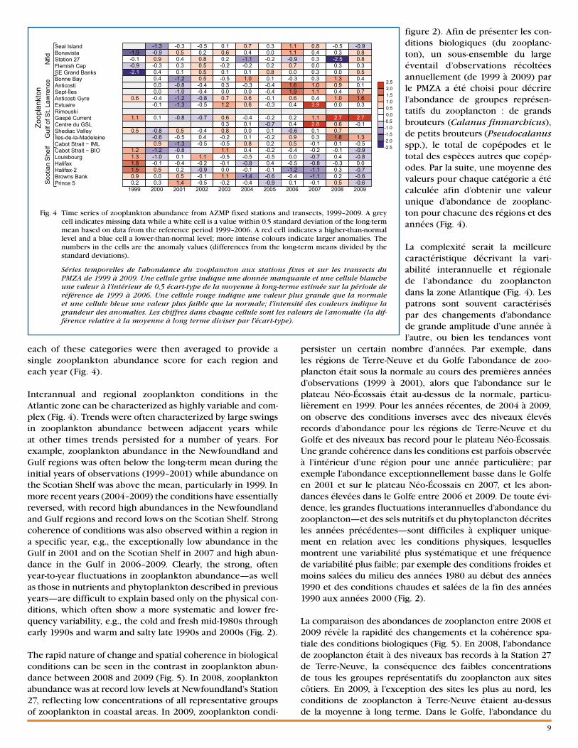
Biological Environment Because much of the effort of the AZMP team over the past year was directed to the 10th year synthesis workshop in March 2010, analysis of some of the chemical and biological variables and standard reports (Research Documents and Science Advisory Reports) were not completed. As a con-sequence, only zooplankton conditions and trends will be summarized in this year’s environmental overview. Like last year, we have adopted the “scorecard” approach that has been employed in previous years to describe physi-cal conditions in the Northwest Atlantic (see Fig. 2). For describing the biological (zooplankton) conditions, a subset of the broad spectrum of observations collected annually (1999–2009) by AZMP was chosen to describe the abun-dance of representative groups of zooplankton: large graz-ers (Calanus finmarchicus), small grazers (Pseudocalanus spp.), total copepods, and non-copepods. The scores for

fement considérant les anomalies positives observées en 2008 (au-dessus de 0,7 écart-type dans les deux cas). Bien que la température minimum de la CIF dans le Golfe ait été près de la normale (–0,2 écart-type), il s’agit d’un réchauffement par rapport à l’anomalie de –0,7 écart-type observée l’été précé-dent. Donc, les trois indices montrent une tendance vers des conditions plus chaudes relativement à 2008. Le volume de la CIF du plateau Néo-Écossais, qui est fortement influencé par la décharge du golfe du Saint-Laurent, a également diminué de manière significative depuis 2008, alors qu’il était de 1,6 écart-types au-dessus de la normale, et était près de la normale (–0,1 écart-type) en 2009. En contrepartie, la superficie de la section transversale de la CIF (T < 0°C) sur les lignes 47°N, Bonavista, White Bay et Seal Island a augmenté, passant de –1,0, –1,4, –0,6 et 0,0 écart-type en 2008, respectivement, à –0,2, –0,4, 0,3 et 0,6 écart-type en 2009.

En 2009, les températures au fond étaient toujours au-dessus de la normale dans les aires les plus au nord (2J et 3K), près de la normale (en deçà de 0,5 écart-type) pour 3Ps, 3LNO, 4V, 4W, 4X, et bien au-dessus de la normale dans 4T. Par rapport à 2008, le réchauffement était significatif (de ~0,7 à 2,2 écart-types) dans les aires 3Ps, 4W et 4T.

En résumé, les températures de l’air aux six points de mesures étaient au-dessus de la normale de plus de 0,5 écart-type. L’indice NAO et les volumes de glace étaient en deçà de 0,5 écart-type de la normale. Les indices de superficie de la sec-tion transversale de la CIF montrent un refroidissement au sud des plateaux du Labrador et de Terre-Neuve depuis 2008, mais en 2009 toutes les régions étaient en deçà de 0,5 écart-type de la normale à l’exception de Seal Island où la superficie était de 0,6 écart-type au-dessus de la normale. Des conditions plus chaudes que la normale prévalaient pour le volume de la CIF dans le golfe du Saint-Laurent et la superficie d’eau froide (T < 1°C) au fond dans le sud du Golfe, mais la température minimale de la CIF du Golfe et le volume de la CIF du plateau Néo-Écossais étaient en deçà de 0,5 écart-type de la normale. Un réchauffement significatif (de 0,7 à 2,2 écart-types) est sur-venu de 2008 à 2009 dans les eaux de fond au banc Saint-Pierre (3Ps), au centre du plateau Néo-Écossais (4W), et dans le sud du golfe (4T). Au total, 26 indices environnementaux décriv-ent les caractéristiques de la température de l’eau de la zone du PMZA (glace; moyenne entre 0 et 100 m; volumes hivernaux d’eau froide; surfaces, volumes et température minimale de la CIF en été; et températures au fond). De ceux-ci, 18 montrent des valeurs en deçà de la normale, sept des valeurs au-dessus de la normale et seulement une valeur sous la normale.

Environnement biologiqueL’équipe du PMZA a été occupée au cours de la dernière année dans la préparation de l’atelier de synthèse soulignant les 10 ans du programme en mars 2010, de sorte que des anal-yses sur des variables chimiques et biologiques et les rapports habituels (Documents de recherche et Avis scientifiques) n’ont pu être complétés pour cet aperçu. Conséquemment, seulement les conditions et les tendances pour le zooplanc-ton seront présentées ici. Encore cette année, nous avons opté pour un tableau synoptique à la manière de l’approche utilisée ces dernières années pour la description des condi-tions physiques dans l’Atlantique Nord-Ouest (se référer à la

9

each of these categories were then averaged to provide a single zooplankton abundance score for each region and each year (Fig. 4).

Interannual and regional zooplankton conditions in the Atlantic zone can be characterized as highly variable and com-plex (Fig. 4). Trends were often characterized by large swings in zooplankton abundance between adjacent years while at other times trends persisted for a number of years. For example, zooplankton abundance in the Newfoundland and Gulf regions was often below the long-term mean during the initial years of observations (1999–2001) while abundance on the Scotian Shelf was above the mean, particularly in 1999. In more recent years (2004–2009) the conditions have essentially reversed, with record high abundances in the Newfoundland and Gulf regions and record lows on the Scotian Shelf. Strong coherence of conditions was also observed within a region in a specific year, e.g., the exceptionally low abundance in the Gulf in 2001 and on the Scotian Shelf in 2007 and high abun-dance in the Gulf in 2006–2009. Clearly, the strong, often year-to-year fluctuations in zooplankton abundance—as well as those in nutrients and phytoplankton described in previous years—are difficult to explain based only on the physical con-ditions, which often show a more systematic and lower fre-quency variability, e.g., the cold and fresh mid-1980s through early 1990s and warm and salty late 1990s and 2000s (Fig. 2).

The rapid nature of change and spatial coherence in biological conditions can be seen in the contrast in zooplankton abun-dance between 2008 and 2009 (Fig. 5). In 2008, zooplankton abundance was at record low levels at Newfoundland’s Station 27, reflecting low concentrations of all representative groups of zooplankton in coastal areas. In 2009, zooplankton condi-

figure 2). Afin de présenter les con-ditions biologiques (du zooplanc-ton), un sous-ensemble du large éventail d’observations récoltées annuellement (de 1999 à 2009) par le PMZA a été choisi pour décrire l’abondance de groupes représen-tatifs du zooplancton : de grands brouteurs (Calanus finmarchicus), de petits brouteurs (Pseudocalanus spp.), le total de copépodes et le total des espèces autres que copép-odes. Par la suite, une moyenne des valeurs pour chaque catégorie a été calculée afin d’obtenir une valeur unique d’abondance de zooplanc-ton pour chacune des régions et des années (Fig. 4).

La complexité serait la meilleure caractéristique décrivant la vari-abilité interannuelle et régionale de l’abondance du zooplancton dans la zone Atlantique (Fig. 4). Les patrons sont souvent caractérisés par des changements d’abondance de grande amplitude d’une année à l’autre, ou bien les tendances vont

persister un certain nombre d’années. Par exemple, dans les régions de Terre-Neuve et du Golfe l’abondance de zoo-plancton était sous la normale au cours des premières années d’observations (1999 à 2001), alors que l’abondance sur le plateau Néo-Écossais était au-dessus de la normale, particu-lièrement en 1999. Pour les années récentes, de 2004 à 2009, on observe des conditions inverses avec des niveaux élevés records d’abondance pour les régions de Terre-Neuve et du Golfe et des niveaux bas record pour le plateau Néo-Écossais. Une grande cohérence dans les conditions est parfois observée à l’intérieur d’une région pour une année particulière; par exemple l’abondance exceptionnellement basse dans le Golfe en 2001 et sur le plateau Néo-Écossais en 2007, et les abon-dances élevées dans le Golfe entre 2006 et 2009. De toute évi-dence, les grandes fluctuations interannuelles d’abondance du zooplancton—et des sels nutritifs et du phytoplancton décrites les années précédentes—sont difficiles à expliquer unique-ment en relation avec les conditions physiques, lesquelles montrent une variabilité plus systématique et une fréquence de variabilité plus faible; par exemple des conditions froides et moins salées du milieu des années 1980 au début des années 1990 et des conditions chaudes et salées de la fin des années 1990 aux années 2000 (Fig. 2).

La comparaison des abondances de zooplancton entre 2008 et 2009 révèle la rapidité des changements et la cohérence spa-tiale des conditions biologiques (Fig. 5). En 2008, l’abondance de zooplancton était à des niveaux bas records à la Station 27 de Terre-Neuve, la conséquence des faibles concentrations de tous les groupes représentatifs du zooplancton aux sites côtiers. En 2009, à l’exception des sites les plus au nord, les conditions de zooplancton à Terre-Neuve étaient au-dessus de la moyenne à long terme. Dans le Golfe, l’abondance du

Fig. 4 Time series of zooplankton abundance from AZMP fixed stations and transects, 1999–2009. A grey cell indicates missing data while a white cell is a value within 0.5 standard deviation of the long-term mean based on data from the reference period 1999–2006. A red cell indicates a higher-than-normal level and a blue cell a lower-than-normal level; more intense colours indicate larger anomalies. The numbers in the cells are the anomaly values (differences from the long-term means divided by the standard deviations).

Séries temporelles de l'abondance du zooplancton aux stations fixes et sur les transects du PMZA de 1999 à 2009. Une cellule grise indique une donnée manquante et une cellule blanche une valeur à l’intérieur de 0,5 écart-type de la moyenne à long-terme estimée sur la période de référence de 1999 à 2006. Une cellule rouge indique une valeur plus grande que la normale et une cellule bleue une valeur plus faible que la normale; l’intensité des couleurs indique la grandeur des anomalies. Les chiffres dans chaque cellule sont les valeurs de l’anomalie (la dif-férence relative à la moyenne à long terme diviser par l’écart-type).

0

1

Seal IslandBonavistaStation 27Flemish CapSE Grand Banks

Nfld

Bonne BayAnticostiSept-ÎlesAnticosti GyreEstuaireRimouskiGaspé CurrentCentre du GSLShediac ValleyÎles-de-la-MadeleineCabot Strait − IML

Zoop

lank

ton

Gul

f of S

t. La

wre

nce

Cabot Strait − BIOLouisbourgHalifaxHalifax-2Browns BankPrince 5S

cotia

n S

helf

-1.3 -0.3 -0.5 0.1 0.7 0.3 1.1 0.8 -0.5 -0.9-1.9 -0.9 0.5 0.2 0.6 0.4 0.0 1.1 0.4 0.3 0.8-0.1 0.9 0.4 0.8 0.2 -1.1 -0.2 -0.9 0.3 -2.5 0.8-0.9 -0.3 0.3 0.5 -0.2 -0.2 0.2 0.7 0.0 0.3 0.3-2.1 0.4 0.1 0.5 0.1 0.1 0.8 0.0 0.3 0.0 0.5

0.4 -1.2 0.5 -0.5 1.0 0.1 -0.3 0.3 1.3 0.40.0 -0.8 -0.4 0.3 -0.3 -0.4 1.6 1.0 0.9 0.10.0 -1.0 -0.4 0.0 0.0 -0.4 1.9 1.1 0.4 0.7

0.6 -0.4 -1.2 -0.8 0.7 0.6 -0.1 0.6 0.4 1.0 1.6-0.1 -1.3 -0.5 1.2 0.6 -0.3 0.4 3.9 0.0 0.3

1.1 0.1 -0.8 -0.7 0.6 -0.4 -0.2 0.2 1.1 2.7 2.70.3 0.1 -0.7 0.4 2.8 0.6 -0.1

0.5 -0.8 0.5 -0.4 0.8 0.0 0.1 -0.6 0.1 0.7-0.6 -0.5 0.4 -0.2 0.1 -0.2 0.9 0.3 1.8 1.30.9 -1.3 -0.5 -0.5 0.8 0.2 0.5 -0.1 0.1 -0.5

1.2 -1.2 -0.8 1.1 0.4 -0.2 -0.4 -0.2 -0.1 -0.91.3 -1.0 0.1 1.1 -0.5 -0.5 -0.5 0.0 -0.7 0.4 -0.81.8 -0.1 -0.4 -0.2 -0.1 -0.8 0.4 -0.5 -0.8 -0.3 0.01.5 0.5 0.2 -0.9 0.0 -0.1 -0.1 -1.2 -1.1 0.3 -0.70.9 0.0 0.5 -0.1 1.1 -1.4 -0.6 -0.4 -1.1 0.2 -0.60.2 0.3 1.4 -0.5 -0.2 -0.4 -0.9 0.1 -0.1 0.5 -0.6

1999 2000 2001 2002 2003 2004 2005 2006 2007 2008 2009

0.0

2.52.01.51.00.5

-2.5-2.0-1.5-1.0-0.5

10

tions in Newfoundland were above the long-term average at all but the most northern site. In the Gulf, zooplankton abundance was well above average at all locations in 2008 and all but the most southern site in 2009. The highest levels were seen in the Gaspé Current and Îles-de-la-Madeleine in both years and attributed largely to an elevated abundance of Pseudocalanus spp. On the Scotian Shelf, zooplankton abun-dance was close to the long-term average, with levels slightly below and slightly above the average at the northernmost and southernmost sites, respectively. In 2009, however, zooplank-ton abundance (all representative groups) was below the aver-age at all sites and similar to the low levels prevailing during the 2004–2007 period.

HighlightsChemical and biological (lower trophic level) conditions in the NW Atlantic are highly variable in space and time, making it a challenge to understand the linkages between physical, chemical, and biological properties and to forecast changes on the annual time scale. Despite this inherent variability, coherent signals that affect broad areas or that persist for sev-eral years have become apparent. For example, zooplankton in the Newfoundland and Gulf regions have exhibited above-average abundance for the past 4–5 years while conditions on the Scotain Shelf have been below the average over the same period. It is tempting to link these larger-scale, longer-term biological trends to comparable-scale, low frequency atmo-sphere–ocean processes. Are the geographically out-of-phase trends in zooplankton abundance we have observed associat-ed with similar phase differences in ocean hydrography (tem-perature and salinity) driven by large-scale meteorological forcing (NAO) (Petrie 2007)? Linking ocean physics, chem-istry, and biology at the smaller spatial and temporal scales is more problematic, e.g., significant changes in zooplankton abundance between 2008 and 2009 were seen at Station 27 and at most sites on the Scotian Shelf while composite physi-

zooplancton était bien au-dessus de la normale à tous les sites en 2008 et en 2009 sauf pour les sites les plus au sud. Pour les deux années, les abondances les plus élevées ont été observées dans le courant de Gaspé et aux Îles-de-la-Madeleine, en grande partie en raison de l’abondance élevée de Pseudocalanus spp. Sur le plateau Néo-Écossais, l’abondance de zooplancton était près de la normale, avec des niveaux légèrement au-dessous ou au-dessus de la normale respectivement aux sites les plus au nord et les plus au sud. Toutefois, en 2009, l’abondance du zoo-plancton (tous les groupes représentés) était sous la normale à tous les sites et était semblable aux bas niveaux qui prévalaient au cours des années 2004 à 2007.

Faits saillantsLes conditions chimiques et biologiques (les niveaux tro-phiques inférieurs) dans l’Atlantique Nord-Ouest sont très variables dans l’espace et le temps ce qui rend difficile la détection de changements à court terme ou régionaux dans l’état ou les abondances spécifiques. Malgré cette variabilité inhérente, des signaux cohérents affectant de grandes sur-faces ou qui ont persisté plusieurs années sont apparents. Par exemple, le zooplancton des régions de Terre-Neuve et du Golfe montre des abondances au-dessus de la moyenne au cours des quatre à cinq dernières années, alors qu’au cours de la même période les conditions sur le plateau Néo-Écossais étaient sous la moyenne. Il est tentant de lier les tendances biologiques à grande échelle et à long terme avec les proces-sus océaniques-atmosphériques de basse fréquence agissant sur une échelle comparable. Ainsi, est-ce que les tendances déphasées géographiquement observées dans l’abondance du zooplancton sont associées à des oppositions de phases semblables dans l’hydrographie (température et salinité) en réponse à un forçage météorologique à grande échelle (NAO) (Petrie 2007)? Il est plus difficile de lier la physique, la chimie et la biologie des océans à de plus petites échelles spatiales et temporelles; par exemple, des changements significatifs de

Fig. 5 Zonal summary of the average annual anomalies for zooplankton for 2008 and 2009 (NL=Newfoundland Shelf, GSL=Gulf of St. Lawrence, SS=Scotian Shelf/Bay of Fundy).

Sommaire pour la zone des anomalies moyennes annuelles pour le zooplancton en 2008 et 2009 (NL=plateau de Terre-Neuve, GSL=golfe du Saint-Laurent, SS= plateau Néo-Écossais/baie de Fundy).

-3 -2 -1 0 1 2 3

Seal IslandBonavista Bay

Station 27Flemish Cap

SE Grand BanksBonne Bay

AnticostiSept-Îles

Anticosti GyreEstuaire

Gaspé CurrentShediac Valley

Central GulfÎles-de-la-Madeleine

Cabot Strait − IMLCabot Strait − BIO

LouisbourgHalifax

Halifax 2Browns Bank

P-5

2008

Average Anomaly / Anomalie moyenne

Zooplankton / Zooplancton

NL

GSL

SS

Seal IslandBonavista Bay

Station 27Flemish Cap

SE Grand BanksBonne Bay

AnticostiSept-Îles

Anticosti GyreEstuaire

Gaspé CurrentShediac Valley

Central GulfÎles-de-la-Madeleine

Cabot Strait − IMLCabot Strait − BIO

LouisbourgHalifax

Halifax 2Browns Bank

P-5

-3 -2 -1 0 1 2 3

2009

Average Anomaly / Anomalie moyenne

Zooplankton / Zooplancton

NL

GSL

SS

11

l’abondance du zooplancton ont été observés entre 2008 et 2009 à la Station 27 et à la plupart des sites sur le plateau Néo-Écossais, alors que les propriétés physiques montraient peu de changements entre 2008 et 2009 (Fig. 2) et sont demeurées bien en deçà des normales. Une meilleure connaissance des processus agissant à courte échelle temporelle (du journalier au saisonnier) est requise afin de comprendre les interac-tions à l’échelle d’une année entre la physique, la chimie et la biologie. Par exemple, comment les changements saisonniers dans le développement des structures hydrographiques du niveau supérieur de la colonne d’eau (soit la stratification) influence l’apport de nutriments, la croissance du phytoplanc-ton—incluant le moment et l’importance de la floraison—et comment la croissance du phytoplancton à son tour influence la phénologie du zooplancton, soit le moment de la reproduc-tion, la survie des stades de développement et l’entrée en diapause? Le PMZA permet d’obtenir les observations aux échelles appropriées afin de commencer à répondre à ces questions importantes.

cal properties changed little between 2008 and 2009 (Fig. 2) and were largely within normal limits. Understanding physical, chemical, and biological interactions on annual time scales will require a better knowledge of processes on shorter time scales (daily to seasonal). How, for example, do changes in the seasonal development of the upper water-col-umn hydrographic structure (i.e., stratification) influence the nutrient supply for phytoplankton growth, timing, and mag-nitude of phytoplankton blooms, and how do phytoplankton growth dynamics in turn influence zooplankton phenology, such as timing of reproduction, survival of developmental stages, and diapause? AZMP provides observations at the appropriate scales and the cumulative data to begin to tackle these important questions.

ReferencePetrie, B. 2007. Does the North Atlantic Oscillation affect hydro-

graphic properties on the Canadian Atlantic continental shelf? Atmos.-Ocean 45(3): 141-151 doi:10.3137/ao.450302.

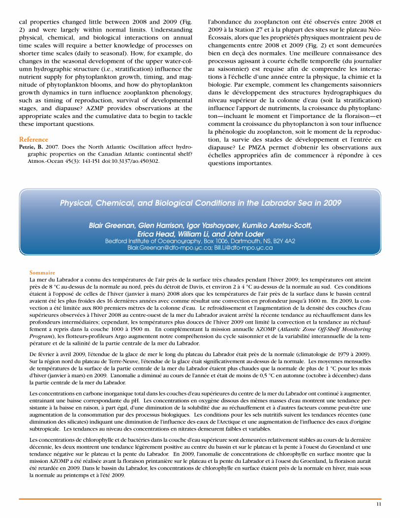
SommaireLa mer du Labrador a connu des températures de l’air près de la surface très chaudes pendant l’hiver 2009; les températures ont atteint près de 8 °C au-dessus de la normale au nord, près du détroit de Davis, et environ 2 à 4 °C au-dessus de la normale au sud. Ces conditions étaient à l'opposé de celles de l’hiver (janvier à mars) 2008 alors que les températures de l’air près de la surface dans le bassin central avaient été les plus froides des 16 dernières années avec comme résultat une convection en profondeur jusqu’à 1600 m. En 2009, la con-vection a été limitée aux 800 premiers mètres de la colonne d’eau. Le refroidissement et l’augmentation de la densité des couches d’eau supérieures observées à l’hiver 2008 au centre-ouest de la mer du Labrador avaient arrêté la récente tendance au réchauffement dans les profondeurs intermédiaires; cependant, les températures plus douces de l’hiver 2009 ont limité la convection et la tendance au réchauf-fement a repris dans la couche 1000 à 1500 m. En complémentant la mission annuelle AZOMP (Atlantic Zone Off-Shelf Monitoring Program), les flotteurs-profileurs Argo augmentent notre compréhension du cycle saisonnier et de la variabilité interannuelle de la tem-pérature et de la salinité de la partie centrale de la mer du Labrador.

De février à avril 2009, l’étendue de la glace de mer le long du plateau du Labrador était près de la normale (climatologie de 1979 à 2009). Sur la région nord du plateau de Terre-Neuve, l’étendue de la glace était significativement au-dessus de la normale. Les moyennes mensuelles de températures de la surface de la partie centrale de la mer du Labrador étaient plus chaudes que la normale de plus de 1 °C pour les mois d’hiver (janvier à mars) en 2009. L’anomalie a diminué au cours de l’année et était de moins de 0,5 °C en automne (octobre à décembre) dans la partie centrale de la mer du Labrador.

Les concentrations en carbone inorganique total dans les couches d’eau supérieures du centre de la mer du Labrador ont continué à augmenter, entrainant une baisse correspondante du pH. Les concentrations en oxygène dissous des mêmes masses d’eau montrent une tendance per-sistante à la baisse en raison, à part égal, d’une diminution de la solubilité due au réchauffement et à d’autres facteurs comme peut-être une augmentation de la consommation par des processus biologiques. Les conditions pour les sels nutritifs suivent les tendances récentes (une diminution des silicates) indiquant une diminution de l’influence des eaux de l’Arctique et une augmentation de l’influence des eaux d’origine subtropicale. Les tendances au niveau des concentrations en nitrates demeurent faibles et variables.

Les concentrations de chlorophylle et de bactéries dans la couche d’eau supérieure sont demeurées relativement stables au cours de la dernière décennie, les deux montrent une tendance légèrement positive au centre du bassin et sur le plateau et la pente à l’ouest du Groenland et une tendance négative sur le plateau et la pente du Labrador. En 2009, l’anomalie de concentrations de chlorophylle en surface montre que la mission AZOMP a été réalisée avant la floraison printanière sur le plateau et la pente du Labrador et à l’ouest du Groenland, la floraison aurait été retardée en 2009. Dans le bassin du Labrador, les concentrations de chlorophylle en surface étaient près de la normale en hiver, mais sous la normale au printemps et à l’été 2009.

Blair Greenan, Glen Harrison, Igor Yashayaev, Kumiko Azetsu-Scott,Erica Head, William Li, and John Loder

Bedford Institute of Oceanography, Box 1006, Dartmouth, NS, B2Y 4A2Blair.Greenan@dfo-mpo.gc.ca; Bill.Li@dfo-mpo.gc.ca

Physical, Chemical, and Biological Conditions in the Labrador Sea in 2009

12

The Atlantic Zone Off-Shelf Monitoring Program (AZOMP), operated by the Science Branch of DFO Maritimes, collects and analyzes physical, chemical, and biological oceanograph-ic observations from the continental slope and deeper waters of the NW Atlantic. Its objective is to monitor variability in the ocean climate and plankton affecting regional climate and ecosystems off Atlantic Canada and the global climate system. AZOMP has three primary components:

• TheLabradorSeaMonitoringProgram,thelargestcompo-nent of AZOMP, collects and analyzes physical, chemical, and biological observations on an oceanographic section across the Labrador Sea, referred to as the AR7W section.

• The Scotian Slope/Rise Monitoring Program collects andanalyzes physical, chemical, and biological observations over the Scotian Slope and Rise at deep-water stations added to the offshore end of AZMP's Halifax line (XHL).

• Temperature and salinity profiles from the Argo FloatProgram are used to complement observations from AR7W and XHL. DFO oceanographic labs contribute to the International Argo Program, which has over 3000 subsur-face floats drifting in the world's ocean and profiling from the surface to 2000 m every ten days.

More information on the AZOMP is available on the Web at http://www.bio.gc.ca/monitoring-monitorage/azomp-pmzao/index-eng.htm.

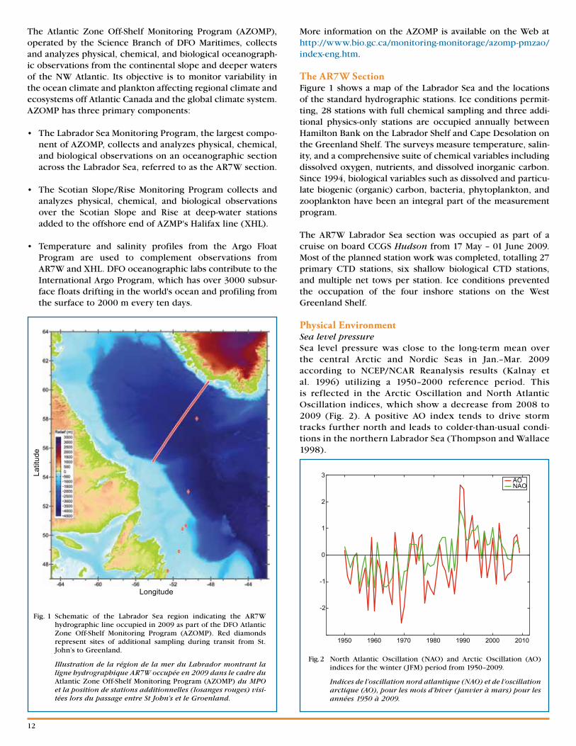
The AR7W SectionFigure 1 shows a map of the Labrador Sea and the locations of the standard hydrographic stations. Ice conditions permit-ting, 28 stations with full chemical sampling and three addi-tional physics-only stations are occupied annually between Hamilton Bank on the Labrador Shelf and Cape Desolation on the Greenland Shelf. The surveys measure temperature, salin-ity, and a comprehensive suite of chemical variables including dissolved oxygen, nutrients, and dissolved inorganic carbon. Since 1994, biological variables such as dissolved and particu-late biogenic (organic) carbon, bacteria, phytoplankton, and zooplankton have been an integral part of the measurement program.

The AR7W Labrador Sea section was occupied as part of a cruise on board CCGS Hudson from 17 May – 01 June 2009. Most of the planned station work was completed, totalling 27 primary CTD stations, six shallow biological CTD stations, and multiple net tows per station. Ice conditions prevented the occupation of the four inshore stations on the West Greenland Shelf.

Physical EnvironmentSea level pressureSea level pressure was close to the long-term mean over the central Arctic and Nordic Seas in Jan.–Mar. 2009 according to NCEP/NCAR Reanalysis results (Kalnay et al. 1996) utilizing a 1950–2000 reference period. This is reflected in the Arctic Oscillation and North Atlantic Oscillation indices, which show a decrease from 2008 to 2009 (Fig. 2). A positive AO index tends to drive storm tracks further north and leads to colder-than-usual condi-tions in the northern Labrador Sea (Thompson and Wallace 1998).

Fig. 1 Schematic of the Labrador Sea region indicating the AR7W hydrographic line occupied in 2009 as part of the DFO Atlantic Zone Off-Shelf Monitoring Program (AZOMP). Red diamonds represent sites of additional sampling during transit from St. John’s to Greenland.

Illustration de la région de la mer du Labrador montrant la ligne hydrographique AR7W occupée en 2009 dans le cadre du Atlantic Zone Off-Shelf Monitoring Program (AZOMP) du MPO et la position de stations additionnelles (losanges rouges) visi-tées lors du passage entre St John’s et le Groenland.

Longitude

Latit

ude

Fig. 2 North Atlantic Oscillation (NAO) and Arctic Oscillation (AO) indices for the winter (JFM) period from 1950–2009.

Indices de l’oscillation nord atlantique (NAO) et de l’oscillation arctique (AO), pour les mois d’hiver (janvier à mars) pour les années 1950 à 2009.

AONAO

3

2

1

0

-1

-2

1950 1960 1970 1980 1990 2000 2010

13

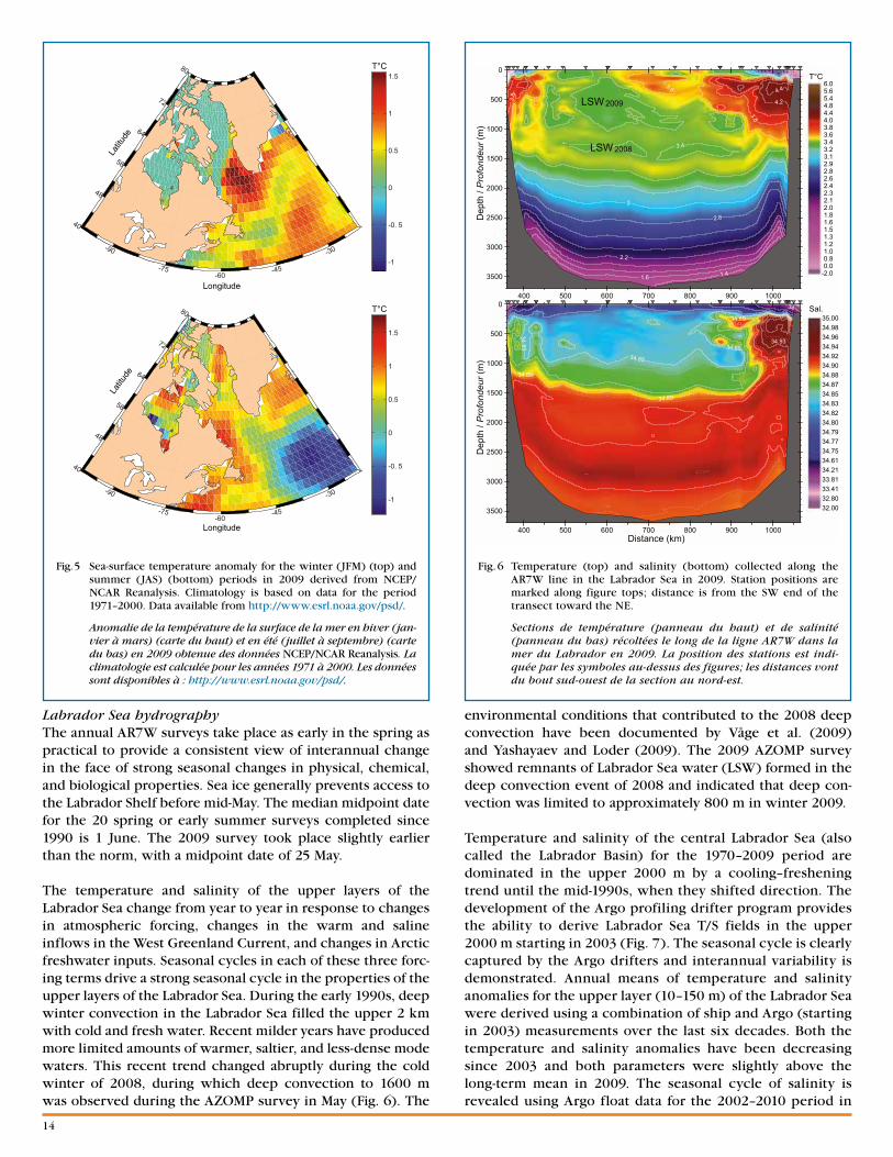
Surface air temperatureWinter 2009 (defined as January–February–March, JFM) surface air temperatures over the Labrador Sea were warm-er than normal while summer ( July–August–September, JAS) temperatures were near normal (Fig. 3). The refer-ence period for analysis was 1968 to 1996. NCEP Reanalysis results show JFM surface temperatures up to 8°C above normal in southern Davis Strait and the northern Labrador Sea. JFM 2009 surface air temperatures over the central and southern Labrador Sea were 2–4°C above normal. The 2009 annual mean surface air temperature for the north-ern Labrador Sea was approximately 4°C above normal and about 1°C above normal for the southern region. The 2009 winter air temperatures were in strong contrast to those of winter 2008, which was the coldest since 1993 (16 years) and the eighth coldest in the 61-year NCEP Reanalysis (1948–2008) for this region. Winter 2008 temperatures were about 6°C below normal in the northern Labrador Sea and approximately 1.5°C above normal in the southern Labrador Sea. This was a marked change from the previ-ous eight years (2000–2007), when wintertime surface air temperatures averaged 2°C warmer than normal.

Sea ice Sea-ice extent (Fig. 4) is presented as daily sea-ice concentra-tion derived from Nimbus-7 SMMR, DMSP SSM/I, and DMSP SSMIS satellite passive microwave radiances using the NASA Team algorithms (Comiso 1999). The data are gridded on the SSM/I polar stereographic grid with a resolution of 25 × 25 km. The monthly climatology of ice concentration is created using data from 31 years (1979–2009). This analysis indicates that the Feb.–Apr. 2009 extent of sea ice along the Labrador Shelf was close to normal, while on the northern Newfoundland Shelf the 2009 extent was significantly above average.

Sea-surface temperatureLabrador Sea sea-surface temperatures (SST) during JFM 2009 (Fig. 5) indicate that the winter SST in ice-free areas was 0.5–1.5°C above normal (climatology for this data set is 1971–2000). This is consistent with the surface air tempera-tures, which were 2–4°C above normal in the central and southern Labrador Sea during this period. The annual mean anomalies for 2009, which include the underlying seasonal variability, were less than 1°C for the region. In contrast, JFM 2008 SST was the coldest since 2000, consistent with the relatively cold winter conditions and increased sea-ice coverage that occurred that year.

-90

-75-60

-45

-30

40

48

56

64

72

80

-1

0

1

2

3

4

5

6

7

8

-90

-75-60

-45

-30

40

48

56

64

72

80

-1

0

1

2

3

4

Longitude

Longitude

Latitu

de

Latitu

de

T°C

T°C

Fig. 3 Surface air temperature anomaly for the winter (JFM) (top) and summer (JAS) (bottom) periods in 2009 as derived from NCEP/NCAR Reanalysis. Climatology is based on data for the 1968–1996 period. Data available from http://www.esrl.noaa.gov/psd/.

Anomalie des températures de l’air près de la surface en hiver (jan-vier à mars) (carte du haut) et en été (juillet à septembre) (carte du bas) en 2009 obtenue des données NCEP/NCAR Reanalysis. La climatologie est calculée pour les années 1968 à 1996. Les données sont disponibles à : http://www.esrl.noaa.gov/psd/.

Fig. 4 Sea-ice extent; the thin black line shows the 1000 m isobath for reference. The blue line represents the February–April 50% ice concentration averaged over 31 years (1979–2009), and the red line shows the February–April averaged 50% ice concentration in 2009.

Étendue de la glace de mer; la ligne noire mince montre l’isobathe de 1000 m en référence. La ligne bleue montre la concentration à 50 % moyenne, de février à avril, sur 31 ans (1979 à 2009), et la ligne rouge montre la concentration à 50 %, de février à avril, en 2009.

-70 -65 -60 -55 -50 -45

65

60

55

50

45

Longitude

Latit

ude

14

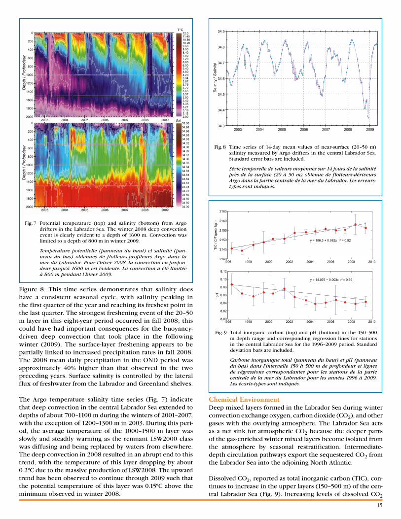
environmental conditions that contributed to the 2008 deep convection have been documented by Våge et al. (2009) and Yashayaev and Loder (2009). The 2009 AZOMP survey showed remnants of Labrador Sea water (LSW) formed in the deep convection event of 2008 and indicated that deep con-vection was limited to approximately 800 m in winter 2009.

Temperature and salinity of the central Labrador Sea (also called the Labrador Basin) for the 1970–2009 period are dominated in the upper 2000 m by a cooling–freshening trend until the mid-1990s, when they shifted direction. The development of the Argo profiling drifter program provides the ability to derive Labrador Sea T/S fields in the upper 2000 m starting in 2003 (Fig. 7). The seasonal cycle is clearly captured by the Argo drifters and interannual variability is demonstrated. Annual means of temperature and salinity anomalies for the upper layer (10–150 m) of the Labrador Sea were derived using a combination of ship and Argo (starting in 2003) measurements over the last six decades. Both the temperature and salinity anomalies have been decreasing since 2003 and both parameters were slightly above the long-term mean in 2009. The seasonal cycle of salinity is revealed using Argo float data for the 2002–2010 period in

Labrador Sea hydrographyThe annual AR7W surveys take place as early in the spring as practical to provide a consistent view of interannual change in the face of strong seasonal changes in physical, chemical, and biological properties. Sea ice generally prevents access to the Labrador Shelf before mid-May. The median midpoint date for the 20 spring or early summer surveys completed since 1990 is 1 June. The 2009 survey took place slightly earlier than the norm, with a midpoint date of 25 May.

The temperature and salinity of the upper layers of the Labrador Sea change from year to year in response to changes in atmospheric forcing, changes in the warm and saline inflows in the West Greenland Current, and changes in Arctic freshwater inputs. Seasonal cycles in each of these three forc-ing terms drive a strong seasonal cycle in the properties of the upper layers of the Labrador Sea. During the early 1990s, deep winter convection in the Labrador Sea filled the upper 2 km with cold and fresh water. Recent milder years have produced more limited amounts of warmer, saltier, and less-dense mode waters. This recent trend changed abruptly during the cold winter of 2008, during which deep convection to 1600 m was observed during the AZOMP survey in May (Fig. 6). The

Fig. 5 Sea-surface temperature anomaly for the winter (JFM) (top) and summer (JAS) (bottom) periods in 2009 derived from NCEP/NCAR Reanalysis. Climatology is based on data for the period 1971–2000. Data available from http://www.esrl.noaa.gov/psd/.

Anomalie de la température de la surface de la mer en hiver (jan-vier à mars) (carte du haut) et en été (juillet à septembre) (carte du bas) en 2009 obtenue des données NCEP/NCAR Reanalysis. La climatologie est calculée pour les années 1971 à 2000. Les données sont disponibles à : http://www.esrl.noaa.gov/psd/.

-90

-75-60

-45

-30

40

48

56

64

72

80

-1

-0. 5

0

0.5

1

1.5

-90

-75-60

-45

-30

40

48

56

64

72

80

-1

-0. 5

0

0.5

1

1.5

T°C

T°C

Longitude

Longitude

Latitu

de

Latitu

de

Fig. 6 Temperature (top) and salinity (bottom) collected along the AR7W line in the Labrador Sea in 2009. Station positions are marked along figure tops; distance is from the SW end of the transect toward the NE.

Sections de température (panneau du haut) et de salinité (panneau du bas) récoltées le long de la ligne AR7W dans la mer du Labrador en 2009. La position des stations est indi-quée par les symboles au-dessus des figures; les distances vont du bout sud-ouest de la section au nord-est.

1.41.6

2.2

2.2

2.8

3

3

3.4

3.6

3.8

3.8

4.2

4.4

34

34.85

34.85

34.85

34.89

34.89

34.89

34.93

400 500 600 700 800 900 1000

3500

3000

2500

2000

1500

1000

500

0

Dep

th /

Pro

fond

eur (

m)

LSW 2008

LSW 2009

400 500 600 700 800 900 1000Distance (km)

3500

3000

2500

2000

1500

1000

500

0

Dep

th /

Pro

fond

eur (

m)

35.0034.9834.9634.9434.9234.9034.8834.8734.8534.8334.8234.8034.7934.7734.7534.6134.2133.8133.4132.8032.00

6.05.65.44.84.44.03.83.63.43.23.12.92.82.62.42.32.12.01.81.61.51.31.21.00.80.0

-2.0

T°C

Sal.

15

Chemical EnvironmentDeep mixed layers formed in the Labrador Sea during winter convection exchange oxygen, carbon dioxide (CO2), and other gases with the overlying atmosphere. The Labrador Sea acts as a net sink for atmospheric CO2 because the deeper parts of the gas-enriched winter mixed layers become isolated from the atmosphere by seasonal restratification. Intermediate-depth circulation pathways export the sequestered CO2 from the Labrador Sea into the adjoining North Atlantic.

Dissolved CO2, reported as total inorganic carbon (TIC), con-tinues to increase in the upper layers (150–500 m) of the cen-tral Labrador Sea (Fig. 9). Increasing levels of dissolved CO2

Figure 8. This time series demonstrates that salinity does have a consistent seasonal cycle, with salinity peaking in the first quarter of the year and reaching its freshest point in the last quarter. The strongest freshening event of the 20–50 m layer in this eight-year period occurred in fall 2008; this could have had important consequences for the buoyancy-driven deep convection that took place in the following winter (2009). The surface-layer freshening appears to be partially linked to increased precipitation rates in fall 2008. The 2008 mean daily precipitation in the OND period was approximately 40% higher than that observed in the two preceding years. Surface salinity is controlled by the lateral flux of freshwater from the Labrador and Greenland shelves.

The Argo temperature–salinity time series (Fig. 7) indicate that deep convection in the central Labrador Sea extended to depths of about 700–1100 m during the winters of 2001–2007, with the exception of 1200–1300 m in 2003. During this peri-od, the average temperature of the 1000–1500 m layer was slowly and steadily warming as the remnant LSW2000 class was diffusing and being replaced by waters from elsewhere. The deep convection in 2008 resulted in an abrupt end to this trend, with the temperature of this layer dropping by about 0.2ºC due to the massive production of LSW2008. The upward trend has been observed to continue through 2009 such that the potential temperature of this layer was 0.15ºC above the minimum observed in winter 2008.

Fig. 7 Potential temperature (top) and salinity (bottom) from Argo drifters in the Labrador Sea. The winter 2008 deep convection event is clearly evident to a depth of 1600 m. Convection was limited to a depth of 800 m in winter 2009.

Température potentielle (panneau du haut) et salinité (pan-neau du bas) obtenues de flotteurs-profileurs Argo dans la mer du Labrador. Pour l’hiver 2008, la convection en profon-deur jusqu’à 1600 m est évidente. La convection a été limitée à 800 m pendant l’hiver 2009.

2003 2004 2005 2006 2007 2008 2009

2000

1800

1600

1400

1200

1000

800

600

400

200

0

Dep

th /

Pro

fond

eur

2003 2004 2005 2006 2007 2008 2009

2000

1800

1600

1400

1200

1000

800

600

400

200

0

Dep

th /

Pro

fond

eur

12.011.4010.8010.209.609.008.407.807.206.606.005.404.804.203.943.873.793.723.653.573.503.423.353.273.193.122.90

T°C

Sal.35.0034.9834.9634.9534.9334.9234.9034.8934.8734.8634.8534.8434.8334.8334.8234.8134.7834.7234.6634.6034.5034.30

34.9

34.8

34.7

34.6

34.5

34.4

34.32003 2004 2005 2006 2007 2008 2009

Sal

inity

/ S

alin

ité

Fig. 8 Time series of 14-day mean values of near-surface (20–50 m) salinity measured by Argo drifters in the central Labrador Sea. Standard error bars are included.

Série temporelle de valeurs moyennes sur 14 jours de la salinité près de la surface (20 à 50 m) obtenue de flotteurs-dériveurs Argo dans la partie centrale de la mer du Labrador. Les erreurs-types sont indiqués.

Fig. 9 Total inorganic carbon (top) and pH (bottom) in the 150–500 m depth range and corresponding regression lines for stations in the central Labrador Sea for the 1996–2009 period. Standard deviation bars are included.

Carbone inorganique total (panneau du haut) et pH (panneau du bas) dans l’intervalle 150 à 500 m de profondeur et lignes de régressions correspondantes pour les stations de la parie centrale de la mer du Labrador pour les années 1996 à 2009. Les écarts-types sont indiqués.

1996 1998 2000 2002 2004 2006 2008 20102140

2145

2150

2155

2160

2165

y = 186.3 + 0.982x r2 = 0.92

TIC

/ C

IT (µ

mol

kg-1

)

1996 1998 2000 2002 2004 2006 2008 20108.00

8.02

8.04

8.06

8.08

8.10

8.12

y = 14.076 − 0.003x r2 = 0.69

pH

16

lead to ocean acidification, with potential impacts on marine ecosystems. The concentration of total inorganic carbon in this annually ventilated upper layer has increased by about 12 µmol kg-1 from 1996 to 2009. The corresponding decrease of about 0.03 pH units (Fig. 9) is equivalent to an increase in acidity by nearly 7.5%. If pH continues to decline at this rate, the upper layers of the Labrador Sea will become corrosive to some marine organisms with calcium carbonate shells and skeletons by the latter half of the present century.

Dissolved oxygen continues to show a negative trend in this same central Labrador Sea water mass (Fig. 10). More than half of the decline can be explained by decreases in oxygen solubil-ity associated with the warming of this layer by about 0.8°C over the past 18 years. Removal of this solubility effect gives apparent oxygen utilization (AOU) (Fig. 10), which is the dif-ference between the saturation concentration for the observed temperature and salinity and the observed concentration. Decreased air–sea exchanges of oxygen and a reduction in the transport of oxygen to depth are expected in the milder condi-tions of the recent past. Under these conditions, biological pro-cesses (respiration) will consume oxygen and increase AOU. Any oxygen consumption associated with increased respiration will also increase TIC. Both the continuing global increase in atmospheric CO2 and local biology play a role in the observed TIC increases in the upper layers of the Labrador Sea.

Nutrient concentrations in the Labrador Basin have been estimated using water mass analysis to group the results based on seawater density (Fig. 11). The two examples

Fig. 10 Dissolved oxygen (top) and apparent oxygen utilization (bottom) in the 150–500 m depth range and corresponding regression lines for stations in the central Labrador Sea for the 1990–2009 period. Standard deviation bars are included.

Oxygène dissous (panneau du haut) et l’utilisation apparente d’oxygène (panneau du bas) dans l’intervalle 150 à 500 m de profondeur et lignes de régressions correspondantes pour les stations de la parie centrale de la mer du Labrador pour les années 1990 à 2009. Les écarts-types sont indiqués.

1990 1992 1994 1996 1998 2000 2002 2004 2006 2008 2010285

290

295

300

305

310

315

y = 1693 − 0.698x r2 = 0.7

Oxy

gen

/ Oxy

gène

(µm

ol k

g-1)

1990 1992 1994 1996 1998 2000 2002 2004 2006 2008 201010

15

20

25

30

35

y = -653.7 − 0.339x r2 = 0.35AO

U /

UO

A (µ

mol

kg-1

)

Fig. 11 Nitrate concentrations in Northeast Atlantic deep water (NEADW) and silicate concentrations in Denmark Strait over-flow water (DSOW) with corresponding regression lines. Standard deviation bars are included.

Concentrations en nitrates dans la masse d’eau Northeast Atlantic deep water (NEADW) et en silicates dans la masse d’eau Denmark Strait overflow water (DSOW) et lignes de régressions correspondantes. Les écarts-types sont indiqués.

1990 1992 1994 1996 1998 2000 2002 2004 2006 2008 201014.5

15

15.5

16

16.5

17

17.5

y = -45.3 + 0.031x r2 = 0.72Nitr

ate

/ Nitr

ate

(mm

ol m

-3)

1990 1992 1994 1996 1998 2000 2002 2004 2006 2008 20109

10

11

12

13

y = 123.5 − 0.0.057x r2 = 0.46Sili

cate

/ S

ilice

(mm

ol m

-3)

1996 2000 2004 2008

phyl

l /ph

ylle

g m

-3)

1

Labrador Shelf/Slope (LS)

1996 2000 2004 2008

Labrador Basin (LB)

1996 2000 2004 2008

Greenland Shelf/Slope (GS)

Chl

orop

Chl

oro p

(log

mg

-1

0

11

Pic

ophy

topl

ankt

on /

Pic

ophy

topl

anct

on

(log

cel

ls m

-3)

9

10

8

hyto

plan

kton

/h y

topl

anct

once

lls m

-3) 10

11

Nan

oph

Nan

oph

(l

og c

8

9

13

Bac

teria

/B

acté

ries

(log

cells

m-3)

11

12

1996 2000 2004 2008 1996 2000 2004 20081996 2000 2004 2008

Fig. 12 Mean upper layer (0–100 m) concentrations of chlorophyll, picophytoplankton, nanophytoplankton, and bacteria averaged over groups of stations (showing standard deviations) for the Labrador Shelf/Slope (LS), the central Labrador Basin (LB), and the Greenland Shelf/Slope (GS). Linear regressions indicate trends but are not statistically significant (p>0.05).

Moyennes et écarts-types des concentrations de chloro phylle, picophytoplancton, nanophytoplancton et des bactéries dans la couche supérieure (0 à 100 m) pour des groupes de sta-tions du plateau et de la pente du Labrador (LS), la partie centrale du bassin du Labrador (LB) et le plateau et la pente du Groenland (GS). Les lignes de régressions montrent les tendances mais ne sont pas significatives (p > 0.05).

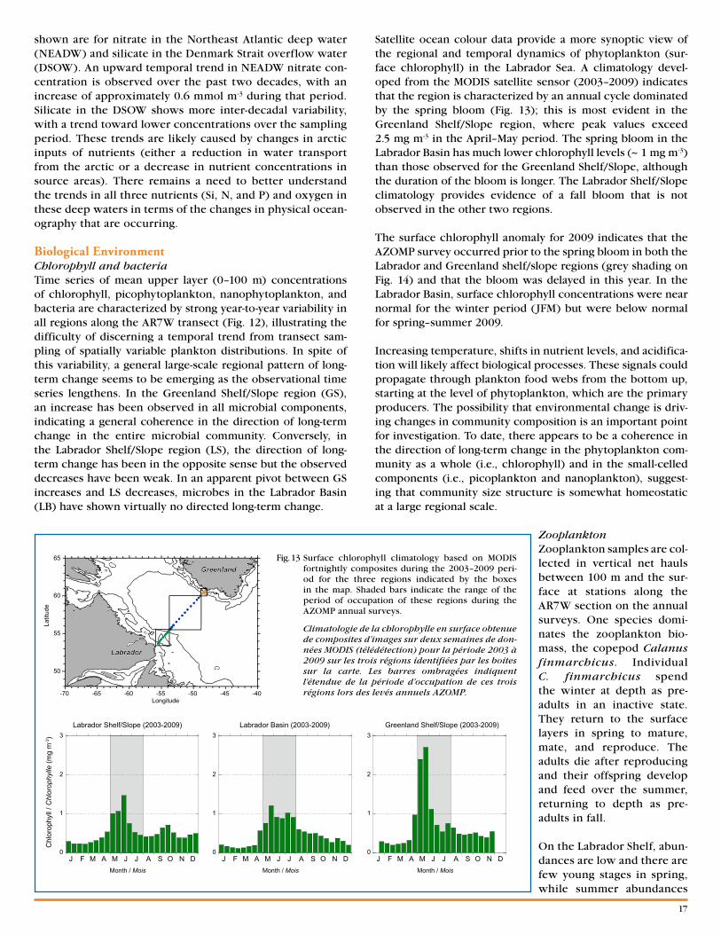
17

shown are for nitrate in the Northeast Atlantic deep water (NEADW) and silicate in the Denmark Strait overflow water (DSOW). An upward temporal trend in NEADW nitrate con-centration is observed over the past two decades, with an increase of approximately 0.6 mmol m-3 during that period. Silicate in the DSOW shows more inter-decadal variability, with a trend toward lower concentrations over the sampling period. These trends are likely caused by changes in arctic inputs of nutrients (either a reduction in water transport from the arctic or a decrease in nutrient concentrations in source areas). There remains a need to better understand the trends in all three nutrients (Si, N, and P) and oxygen in these deep waters in terms of the changes in physical ocean-ography that are occurring.

Biological EnvironmentChlorophyll and bacteriaTime series of mean upper layer (0–100 m) concentrations of chlorophyll, picophytoplankton, nanophytoplankton, and bacteria are characterized by strong year-to-year variability in all regions along the AR7W transect (Fig. 12), illustrating the difficulty of discerning a temporal trend from transect sam-pling of spatially variable plankton distributions. In spite of this variability, a general large-scale regional pattern of long-term change seems to be emerging as the observational time series lengthens. In the Greenland Shelf/Slope region (GS), an increase has been observed in all microbial components, indicating a general coherence in the direction of long-term change in the entire microbial community. Conversely, in the Labrador Shelf/Slope region (LS), the direction of long-term change has been in the opposite sense but the observed decreases have been weak. In an apparent pivot between GS increases and LS decreases, microbes in the Labrador Basin (LB) have shown virtually no directed long-term change.

Satellite ocean colour data provide a more synoptic view of the regional and temporal dynamics of phytoplankton (sur-face chlorophyll) in the Labrador Sea. A climatology devel-oped from the MODIS satellite sensor (2003–2009) indicates that the region is characterized by an annual cycle dominated by the spring bloom (Fig. 13); this is most evident in the Greenland Shelf/Slope region, where peak values exceed 2.5 mg m-3 in the April–May period. The spring bloom in the Labrador Basin has much lower chlorophyll levels (~ 1 mg m-3) than those observed for the Greenland Shelf/Slope, although the duration of the bloom is longer. The Labrador Shelf/Slope climatology provides evidence of a fall bloom that is not observed in the other two regions.

The surface chlorophyll anomaly for 2009 indicates that the AZOMP survey occurred prior to the spring bloom in both the Labrador and Greenland shelf/slope regions (grey shading on Fig. 14) and that the bloom was delayed in this year. In the Labrador Basin, surface chlorophyll concentrations were near normal for the winter period (JFM) but were below normal for spring–summer 2009.

Increasing temperature, shifts in nutrient levels, and acidifica-tion will likely affect biological processes. These signals could propagate through plankton food webs from the bottom up, starting at the level of phytoplankton, which are the primary producers. The possibility that environmental change is driv-ing changes in community composition is an important point for investigation. To date, there appears to be a coherence in the direction of long-term change in the phytoplankton com-munity as a whole (i.e., chlorophyll) and in the small-celled components (i.e., picoplankton and nanoplankton), suggest-ing that community size structure is somewhat homeostatic at a large regional scale.

ZooplanktonZooplankton samples are col-lected in vertical net hauls between 100 m and the sur-face at stations along the AR7W section on the annual surveys. One species domi-nates the zooplankton bio-mass, the copepod Calanus finmarchicus. Individual C. finmarchicus spend the winter at depth as pre-adults in an inactive state. They return to the surface layers in spring to mature, mate, and reproduce. The adults die after reproducing and their offspring develop and feed over the summer, returning to depth as pre-adults in fall.

On the Labrador Shelf, abun-dances are low and there are few young stages in spring, while summer abundances

Fig. 13 Surface chlorophyll climatology based on MODIS fortnightly composites during the 2003–2009 peri-od for the three regions indicated by the boxes in the map. Shaded bars indicate the range of the period of occupation of these regions during the AZOMP annual surveys.

Climatologie de la chlorophylle en surface obtenue de composites d’images sur deux semaines de don-nées MODIS (télédétection) pour la période 2003 à 2009 sur les trois régions identifiées par les boites sur la carte. Les barres ombragées indiquent l'étendue de la période d’occupation de ces trois régions lors des levés annuels AZOMP. -70 -65 -60 -55 -50 -45 -40

Longitude

Latit

ude

65

60

55

50

0

1

2

3Labrador Shelf/Slope (2003-2009)

J F M A M J J A S O N DMonth / Mois

0

1

2

3Labrador Basin (2003-2009)

J F M A M J J A S O N DMonth / Mois

0

1

2

3Greenland Shelf/Slope (2003-2009)

J F M A M J J A S O N DMonth / Mois

Chl

orop

hyll

/ Chl

orop

hylle

(mg

m-3)

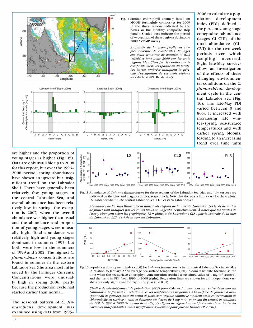
18

are higher and the proportion of young stages is higher (Fig. 15). Data are only available up to 2008 for this report, but over the 1996–2008 period, spring abundances have shown an upward but insig-nificant trend on the Labrador Shelf. There have generally been relatively few young stages in the central Labrador Sea, and overall abundance has been rela-tively low in spring; the excep-tion is 2007, when the overall abundance was higher than usual and the abundance and propor-tion of young stages were unusu-ally high. Total abundance was relatively high and young stages dominant in summer 1995, but both were low in the summers of 1999 and 2002. The highest C. finmarchicus concentrations are found in summer in the eastern Labrador Sea (the area most influ-enced by the Irminger Current). Concentrations were unusual-ly high in spring 2006, partly because the production cycle had started earlier than normal.

The seasonal pattern of C. fin-marchicus development was examined using data from 1995–

2008 to calculate a pop-ulation development index (PDI), defined as the percent young stage copepodite abundance (stages CI–CIII) of the total abundance (CI–CVI) for the two-week periods over which sampling occurred. Eight late-May surveys allow an investigation of the effects of these changing environmen-tal conditions on the C. finmarchicus develop-ment cycle in the cen-tral Labrador Sea (Fig. 16). The late-May PDI varied between 0 and 80%. It increased with increasing late win-ter–spring sea-surface temperatures and with earlier spring blooms, leading to an increasing trend over time until

Abu

ndan

ce /

Abo

ndan

ce(x

1000

m-2

; 0–

100

m) LS CLS ELS

SST (oC)

PD

I (%

)

Day of year / Jour de l’année

Fig. 16 Population development index (PDI) for Calanus finmarchicus in the central Labrador Sea in late May in relation to January–April average sea-surface temperature (left), bloom start date (defined as the time when the sea-surface chlorophyll concentration reached a sustained value of 1 mg m-3 (centre), and the trend in PDI from 1996 to 2008 (right). Regression lines are shown for all independent vari-ables but only significant for day of the year (P < 0.01).

L’Indice de développement de population (PDI) pour Calanus finmarchicus au centre de la mer du Labrador à la fin mai en relation avec les températures moyennes à la surface de janvier à avril (panneau de gauche), date du début de floraison (définie comme le moment où la concentration de chlorophylle en surface atteint et demeure au-dessus de 1 mg m-3) (panneau du centre) et tendance du PDI de 1996 à 2008 (panneau de droite). Les lignes de régression sont présentées pour toutes les variables indépendantes, mais significative seulement pour jour de l'année (P < 0.01)

Fig. 15 Abundance of Calanus finmarchicus for three regions of the Labrador Sea. May and July surveys are indicated by the blue and magenta circles, respectively. Note that the y-axis limits vary for these plots. LS: Labrador Shelf; CLS: central Labrador Sea; ELS: eastern Labrador Sea.

Abondance de Calanus finmarchicus dans trois régions de la mer du Labrador. Les levés de mai et de juillet sont indiqués par les ronds bleus et magenta, respectivement. À noter que les limites de l’axe y changent selon les graphiques. LS = plateau du Labrador ; CLS : partie centrale de la mer du Labrador ; ELS : l’est de la mer du Labrador.

Fig. 14 Surface chlorophyll anomaly based on MODIS fortnightly composites for 2009 in the three regions indicated by the boxes in the monthly composite (top panel). Shaded bars indicate the period of occupation of these regions during the 2009 AZOMP survey.

Anomalie de la chlorophylle en sur-face obtenue de composites d’images sur deux semaines de données MODIS (télédétection) pour 2009 sur les trois régions identifiées par les boites sur le composite mensuel (panneau du haut). Les barres ombrées indiquent la péri-ode d’occupation de ces trois régions lors du levé AZOMP de 2009.

-2

-1

0

1

2Labrador Shelf/Slope (2009)

J F M A M J J A S O N DMonth / Mois

-2

-1

0

1

2Labrador Basin (2009)

J F M A M J J A S O N DMonth / Mois

-2

-1

0

1

2Greenland Shelf/Slope (2009)

J F M A M J J A S O N DMonth / Mois

Chl

orop

hyll

Anom

aly

/C

hlor

ophy

lle A

nom

alie

(mg

m-3)

mg m-3

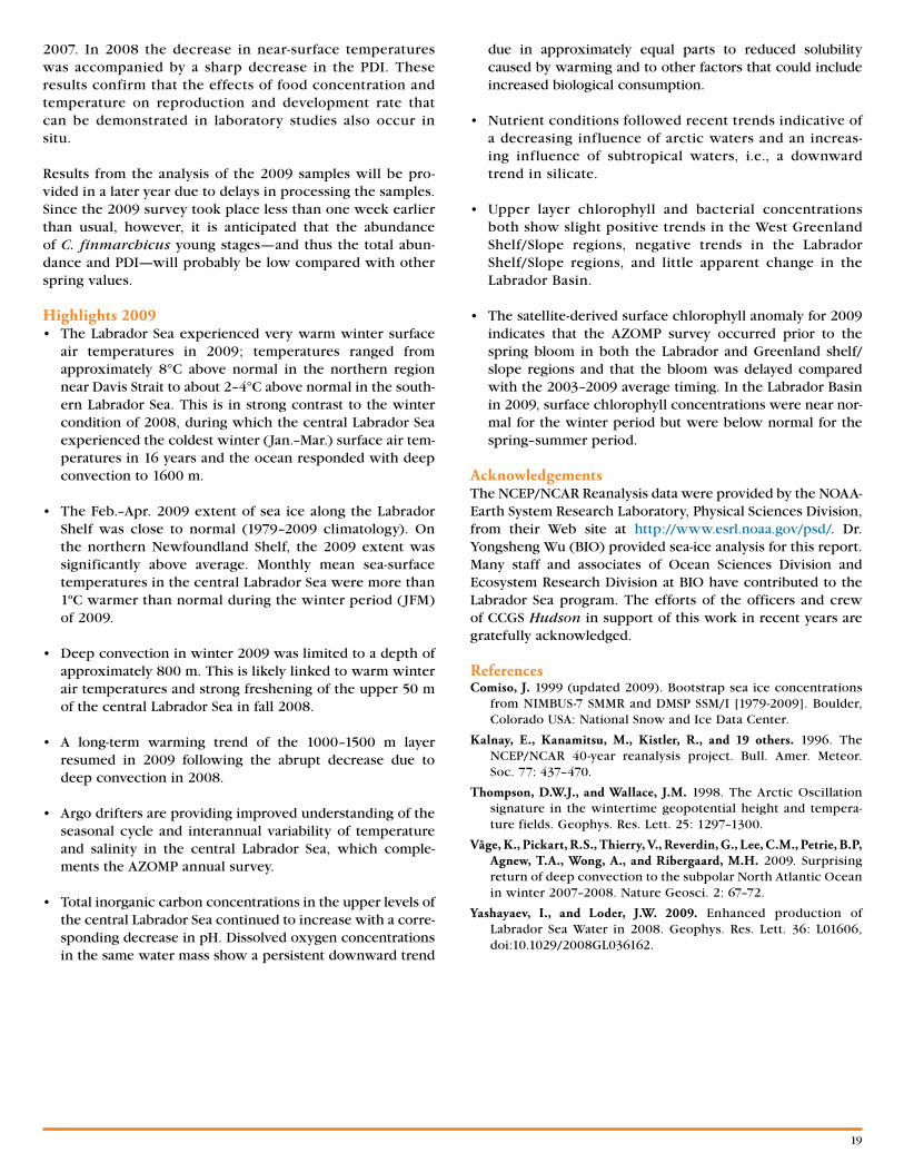
19

2007. In 2008 the decrease in near-surface temperatures was accompanied by a sharp decrease in the PDI. These results confirm that the effects of food concentration and temperature on reproduction and development rate that can be demonstrated in laboratory studies also occur in situ.

Results from the analysis of the 2009 samples will be pro-vided in a later year due to delays in processing the samples. Since the 2009 survey took place less than one week earlier than usual, however, it is anticipated that the abundance of C. finmarchicus young stages—and thus the total abun-dance and PDI—will probably be low compared with other spring values.

Highlights 2009• TheLabradorSeaexperiencedverywarmwinter surface

air temperatures in 2009; temperatures ranged from approximately 8°C above normal in the northern region near Davis Strait to about 2–4°C above normal in the south-ern Labrador Sea. This is in strong contrast to the winter condition of 2008, during which the central Labrador Sea experienced the coldest winter (Jan.–Mar.) surface air tem-peratures in 16 years and the ocean responded with deep convection to 1600 m.

• TheFeb.–Apr.2009extentofsea icealongtheLabradorShelf was close to normal (1979–2009 climatology). On the northern Newfoundland Shelf, the 2009 extent was significantly above average. Monthly mean sea-surface temperatures in the central Labrador Sea were more than 1ºC warmer than normal during the winter period (JFM) of 2009.

• Deepconvectioninwinter2009waslimitedtoadepthofapproximately 800 m. This is likely linked to warm winter air temperatures and strong freshening of the upper 50 m of the central Labrador Sea in fall 2008.

• A long-term warming trend of the 1000–1500 m layerresumed in 2009 following the abrupt decrease due to deep convection in 2008.

• Argodriftersareprovidingimprovedunderstandingoftheseasonal cycle and interannual variability of temperature and salinity in the central Labrador Sea, which comple-ments the AZOMP annual survey.

• Totalinorganiccarbonconcentrationsintheupperlevelsofthe central Labrador Sea continued to increase with a corre-sponding decrease in pH. Dissolved oxygen concentrations in the same water mass show a persistent downward trend

due in approximately equal parts to reduced solubility caused by warming and to other factors that could include increased biological consumption.

• Nutrientconditionsfollowedrecenttrendsindicativeofa decreasing influence of arctic waters and an increas-ing influence of subtropical waters, i.e., a downward trend in silicate.

• Upper layer chlorophyll and bacterial concentrationsboth show slight positive trends in the West Greenland Shelf/Slope regions, negative trends in the Labrador Shelf/Slope regions, and little apparent change in the Labrador Basin.

• Thesatellite-derivedsurfacechlorophyllanomalyfor2009indicates that the AZOMP survey occurred prior to the spring bloom in both the Labrador and Greenland shelf/slope regions and that the bloom was delayed compared with the 2003–2009 average timing. In the Labrador Basin in 2009, surface chlorophyll concentrations were near nor-mal for the winter period but were below normal for the spring–summer period.

AcknowledgementsThe NCEP/NCAR Reanalysis data were provided by the NOAA-Earth System Research Laboratory, Physical Sciences Division, from their Web site at http://www.esrl.noaa.gov/psd/. Dr. Yongsheng Wu (BIO) provided sea-ice analysis for this report. Many staff and associates of Ocean Sciences Division and Ecosystem Research Division at BIO have contributed to the Labrador Sea program. The efforts of the officers and crew of CCGS Hudson in support of this work in recent years are gratefully acknowledged.

ReferencesComiso, J. 1999 (updated 2009). Bootstrap sea ice concentrations

from NIMBUS-7 SMMR and DMSP SSM/I [1979-2009]. Boulder, Colorado USA: National Snow and Ice Data Center.

Kalnay, E., Kanamitsu, M., Kistler, R., and 19 others. 1996. The NCEP/NCAR 40-year reanalysis project. Bull. Amer. Meteor. Soc. 77: 437–470.

Thompson, D.W.J., and Wallace, J.M. 1998. The Arctic Oscillation signature in the wintertime geopotential height and tempera-ture fields. Geophys. Res. Lett. 25: 1297–1300.

Våge, K., Pickart, R.S., Thierry, V., Reverdin, G., Lee, C.M., Petrie, B.P, Agnew, T.A., Wong, A., and Ribergaard, M.H. 2009. Surprising return of deep convection to the subpolar North Atlantic Ocean in winter 2007–2008. Nature Geosci. 2: 67–72.

Yashayaev, I., and Loder, J.W. 2009. Enhanced production of Labrador Sea Water in 2008. Geophys. Res. Lett. 36: L01606, doi:10.1029/2008GL036162.

20

IntroductionThe summertime water column in the Gulf of St. Lawrence consists of three distinct layers: the surface layer, the cold intermediate layer (CIL), and the deeper water layer. Here we focus on the climate variability of the first two layers. Surface temperatures typically reach maximum values from mid-July to mid-August. Gradual cooling occurs thereafter, and wind mixing during the fall leads to a progressively deeper and cool-er surface mixed layer that eventually encompasses the CIL. During winter, the surface layer deepens mostly due to wind-driven mixing prior to ice formation (Galbraith 2006), but also because of buoyancy loss (cooling and reduced run-off) and brine rejection associated with sea-ice formation. The surface winter layer extends to an average depth of 75 m and down to 150 m in some places by the end of March, and exhibits temperatures near freezing (–1.8 to 0°C) (Galbraith 2006). Intruding waters from the Labrador Shelf at the Strait of Belle Isle may extend to the bottom, to depths >200 m in Mécatina Trough. During spring, surface warming, sea-ice melt waters, and continental runoff produce a lower salinity, higher tem-perature surface layer, below which cold winter waters are partly isolated from the atmosphere and become known as the summer CIL. This layer persists until the following winter, warming up and with its temperature minimum deepening gradually during summer (Gilbert and Pettigrew 1997) and more rapidly during the fall as vertical mixing intensifies.

SommaireLes tendances à long terme de la température de la surface de la mer («SST») et de la température de la couche intermédiaire froide (CIF) estivale dans le golfe du Saint-Laurent sont examinés dans cet article. La variabilité interannuelle de la SST durant les mois libres de glace, de mai à novembre, est mesurée à l’aide de données des satellites NOAA obtenues entre 1985 et 2009. À première vue, les changements de la SST affichent un réchauffement moyen de 1,8 °C durant cette période, soit un taux de 7,3 °C par siècle. Ce taux est cependant gonflé par la variabilité interannuelle et pour le démontrer, la moyenne annuelle de la température de l’air mesurée à neuf stations météorologiques situées autour du Golfe, laquelle capture 67% de la variabilité interannuelle de la SST, a servi d’indice représentant la SST pour les années précédant 1985. L’indice annuel de température de l’air est disponible depuis 1945 et est caractérisé par une période relativement stable de 1945 à 1985, suivi d’une période froide qui s’est terminée en 1993. Donc, le début de la prise de données satellitaires coïncide avec une période froide. De plus, les deux années les plus chaudes depuis 1945 sont survenues récemment (en 1999 et 2006) et une seule année depuis 1997 a connu une anomalie négative. Ces facteurs ont tous contribué au taux élevé de réchauffement observé par satellite. Pour remonter plus loin dans le passé, les données (de 1873 à 2009) à trois stations météorologiques autour de Charlottetown sont combinées et démontrent une tendance au réchauffement de l’ordre de 0,78 à 0,9 °C par siècle, tandis que le réchauffement plus continental observé à Pointe-au-Père est de 2,04 ºC par siècle (données de 1876 à 1982). La température de l’air en hiver, quant à elle, affecte le volume de glace produit ainsi que le volume d’eau froide de la couche de surface hivernale mélangée. Comme la couche de surface hivernale forme ce qui deviendra ensuite la CIF estivale, le volume de cette couche a un effet direct sur la température et l’épaisseur de la CIF. Ces trois facteurs océanographiques sont donc reliés à la température de l’air en hiver (r2 de 0,55 à 0,77). De la même façon que pour la température moyenne annuelle, un indice de température hivernale a été construit à partir des données aux neuf stations météorologiques. Il n’y a aucune tendance depuis 1945, mis à part une période froide au début des années 1990 et une forte variabilité interannuelle. La tempéra-ture de l’air en hiver à Charlottetown, quant à elle, démontre une tendance au réchauffement de l’ordre de 1,2 °C par siècle, tandis que le réchauffement observé à Pointe-au-Père demeure encore une fois plus prononcé à 2,4 ºC par siècle. Les conditions hivernales des masses d’eau et de la glace étaient donc fort probablement plus sévères à la fin du 19e siècle que récemment. Bien que l’absence de glace dans le golfe du Saint-Laurent soit probable dans un futur plus ou moins rapproché en raison du réchauffement climatique, la variabilité interan-nuelle du système fait en sorte que le Golfe pourrait être libre de glace une année, mais complètement couvert de glace l’année suivante. En conclusion, les relations entre les températures de l’eau et de l’air, ainsi qu’avec des paramètres océanographiques hivernaux, nous aideront à prévoir l’impact des changements climatiques à venir sur le climat océanographique du golfe du Saint-Laurent.

Sea-Surface TemperatureSea-surface temperature (SST) can shift between warm and cold anomalies in a matter of days to a few weeks; this is the typical timescale of weather patterns that create solar-radiation and air-temperature anomalies that in turn affect SST. This high-frequency variability makes it difficult to use data from oceanographic surveys to study long-term SST vari-ability because these surveys typically cover large areas with a slowly moving vessel once every few months. However, NOAA AVHRR satellite SST data, available since 1985, allow the study of Gulf-wide changes in SST at 1 km resolution because the observations are collected for large areas at the same time and the sampling frequency of the entire Gulf is higher than intrinsic weather variability.

To detect long-term trends in SST over the scale of the Gulf of St. Lawrence, a single yearly mean value is calculated using all pixels within the Gulf (outlined in Fig. 1) from all monthly composites between May and November; these months are always ice-free and therefore typically have valid SST data. The annual means for the Gulf are created from weekly averaged SST composites available from the remote sensing laboratory of DFO’s Maurice Lamontagne Institute. For con-venience, four consecutive weekly images are combined to produce a composite approximating a monthly average (e.g., Fig. 1). The monthly averages still capture mesoscale features

Trends in Sea-Surface and CIL Temperatures in the Gulf of St . Lawrencein Relation to Air Temperature

Peter S . Galbraith1, Pierre Larouche1, Denis Gilbert 1, Joël Chassé 2, and Brian Petrie 31 Institut Maurice-Lamontagne, C.P. 1000, Mont-Joli, QC, G5H 3Z42 Centre des Pêches du Golfe, C.P. 5030, Moncton, NB, E1C 9B6

3 Bedford Institute of Oceanography, Box 1006, Dartmouth, NS, B2Y 4A2peter.galbraith@dfo-mpo.gc.ca

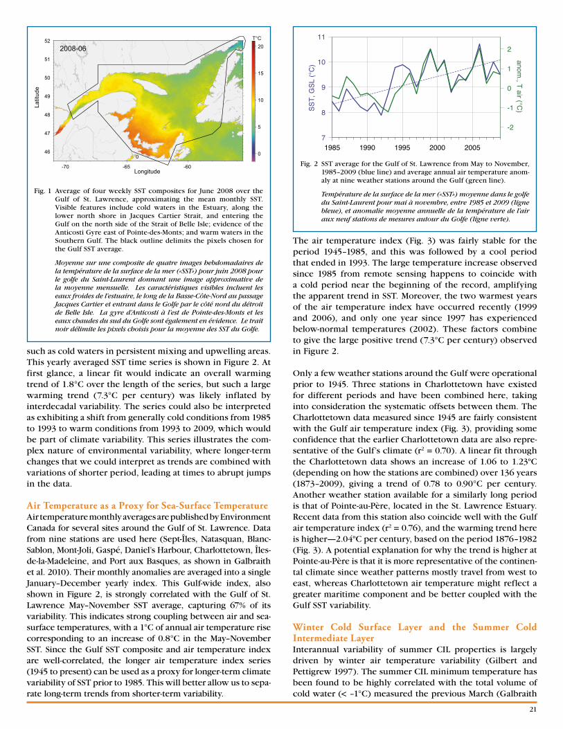
21

such as cold waters in persistent mixing and upwelling areas. This yearly averaged SST time series is shown in Figure 2. At first glance, a linear fit would indicate an overall warming trend of 1.8°C over the length of the series, but such a large warming trend (7.3°C per century) was likely inflated by interdecadal variability. The series could also be interpreted as exhibiting a shift from generally cold conditions from 1985 to 1993 to warm conditions from 1993 to 2009, which would be part of climate variability. This series illustrates the com-plex nature of environmental variability, where longer-term changes that we could interpret as trends are combined with variations of shorter period, leading at times to abrupt jumps in the data.

Air Temperature as a Proxy for Sea-Surface TemperatureAir temperature monthly averages are published by Environment Canada for several sites around the Gulf of St. Lawrence. Data from nine stations are used here (Sept-Îles, Natasquan, Blanc-Sablon, Mont-Joli, Gaspé, Daniel’s Harbour, Charlottetown, Îles-de-la-Madeleine, and Port aux Basques, as shown in Galbraith et al. 2010). Their monthly anomalies are averaged into a single January–December yearly index. This Gulf-wide index, also shown in Figure 2, is strongly correlated with the Gulf of St. Lawrence May–November SST average, capturing 67% of its variability. This indicates strong coupling between air and sea-surface temperatures, with a 1°C of annual air temperature rise corresponding to an increase of 0.8°C in the May–November SST. Since the Gulf SST composite and air temperature index are well-correlated, the longer air temperature index series (1945 to present) can be used as a proxy for longer-term climate variability of SST prior to 1985. This will better allow us to sepa-rate long-term trends from shorter-term variability.

The air temperature index (Fig. 3) was fairly stable for the period 1945–1985, and this was followed by a cool period that ended in 1993. The large temperature increase observed since 1985 from remote sensing happens to coincide with a cold period near the beginning of the record, amplifying the apparent trend in SST. Moreover, the two warmest years of the air temperature index have occurred recently (1999 and 2006), and only one year since 1997 has experienced below-normal temperatures (2002). These factors combine to give the large positive trend (7.3°C per century) observed in Figure 2.

Only a few weather stations around the Gulf were operational prior to 1945. Three stations in Charlottetown have existed for different periods and have been combined here, taking into consideration the systematic offsets between them. The Charlottetown data measured since 1945 are fairly consistent with the Gulf air temperature index (Fig. 3), providing some confidence that the earlier Charlottetown data are also repre-sentative of the Gulf’s climate (r2 = 0.70). A linear fit through the Charlottetown data shows an increase of 1.06 to 1.23ºC (depending on how the stations are combined) over 136 years (1873–2009), giving a trend of 0.78 to 0.90°C per century. Another weather station available for a similarly long period is that of Pointe-au-Père, located in the St. Lawrence Estuary. Recent data from this station also coincide well with the Gulf air temperature index (r2 = 0.76), and the warming trend here is higher—2.04ºC per century, based on the period 1876–1982 (Fig. 3). A potential explanation for why the trend is higher at Pointe-au-Père is that it is more representative of the continen-tal climate since weather patterns mostly travel from west to east, whereas Charlottetown air temperature might reflect a greater maritime component and be better coupled with the Gulf SST variability.

Winter Cold Surface Layer and the Summer Cold Intermediate Layer Interannual variability of summer CIL properties is largely driven by winter air temperature variability (Gilbert and Pettigrew 1997). The summer CIL minimum temperature has been found to be highly correlated with the total volume of cold water (< –1°C) measured the previous March (Galbraith

Fig. 1 Average of four weekly SST composites for June 2008 over the Gulf of St. Lawrence, approximating the mean monthly SST. Visible features include cold waters in the Estuary, along the lower north shore in Jacques Cartier Strait, and entering the Gulf on the north side of the Strait of Belle Isle; evidence of the Anticosti Gyre east of Pointe-des-Monts; and warm waters in the Southern Gulf. The black outline delimits the pixels chosen for the Gulf SST average.

Moyenne sur une composite de quatre images hebdomadaires de la température de la surface de la mer («SST») pour juin 2008 pour le golfe du Saint-Laurent donnant une image approximative de la moyenne mensuelle. Les caractéristiques visibles incluent les eaux froides de l’estuaire, le long de la Basse-Côte-Nord au passage Jacques Cartier et entrant dans le Golfe par le côté nord du détroit de Belle Isle. La gyre d’Anticosti à l’est de Pointe-des-Monts et les eaux chaudes du sud du Golfe sont également en évidence. Le trait noir délimite les pixels choisis pour la moyenne des SST du Golfe.

Fig. 2 SST average for the Gulf of St. Lawrence from May to November, 1985–2009 (blue line) and average annual air temperature anom-aly at nine weather stations around the Gulf (green line).

Température de la surface de la mer («SST») moyenne dans le golfe du Saint-Laurent pour mai à novembre, entre 1985 et 2009 (ligne bleue), et anomalie moyenne annuelle de la température de l’air aux neuf stations de mesures autour du Golfe (ligne verte).

-70 -65 -60

46

47

48

49

50

51

522008-06

Longitude

Latit

ude

T°C

0 0

5

10

15

20

1985 1990 1995 2000 20057

8

9

10

11

SST,

GSL

(°C

)

-2

-1

0

1

2anom

., T air (°C)

22

2006). This is to be expected because the CIL is the remnant of the winter cold surface layer created by winter mixing and convection driven by air tempera-ture and wind. Since sea-ice formation may also reflect cold winter air tem-peratures, one could expect significant correlations between all four of these quantities. Figure 4 shows this strong inter-relationship with the display of a selected index for each parameter. The CIL index chosen here is the volume of water with temperatures below 1°C in the Gulf during the months of August and September. The winter cold water (< –1°C) volume has been sampled every March by a helicopter survey of the Gulf water masses (Galbraith 2006). The ice volume is the maximum recorded every winter based on Canadian Ice Service digitized charts. The winter air temperature is the average January to March air temperature at the same nine stations used above. Note that the scale is reversed for air temperature in Figure 4 because colder temperatures lead to higher ice and cold water volumes. All four time series are further described in Galbraith et al. (2010). There are strong similarities among the four time series, with the squared correlation coeffi-cients varying between 0.55 and 0.77.

Again, air temperature can be used as a proxy for oceanographic parameters, this time the air temperature being the average of January to March values at nine stations over the Gulf (Fig. 5). This average air temperature time series shows no overall trend from 1945 to 2009, except for a longer-than-usual cold period during the early 1990s and strong interannual variability. To exam-ine longer-term variability, we use data from the Charlottetown and Pointe-au-Père weather stations. Correspondence between these stations and the nine-station average is fairly good during the period following 1945. Both locations show a warming trend over the century-scale duration of the time series: an average of 1.6ºC over 135 years (1.2°C per century) at Charlottetown and of 2.4ºC per century at Pointe-au-Père. The warming rates are larger in winter than when considering all months of the year as we did above. The warm-ing trend indicates that past conditions of winter cold-water volume and ice volume and of summer CIL volume and minimum temperature were very likely

Fig. 3 Air temperature index (1945–2009, green line), SST average for the Gulf of St. Lawrence (repeated from Fig. 2; blue line), and air temperature yearly means at three Charlottetown-area stations (black line) and at Point-au-Père (red line). The straight lines represent the linear trends over the entire time series.

Indice des températures de l’air (1945–2009, ligne verte), température de la surface de la mer («SST») moyenne (reprise de la figure 2, ligne bleue), et moyennes annuelles de la tempéra-ture de l’air à trois stations des environs de Charlottetown (ligne noire) et à Pointe-au-Père (ligne rouge). Les lignes droites montrent les tendances linéaires sur les séries complètes.

Fig. 4 Maximum annual ice volume within the Gulf and on the Scotian Shelf, winter cold-water volume, August–September CIL volume, and winter air temperature anomaly in the Gulf of St. Lawrence. Ice volume is estimated from Canadian Ice Service numerical ice charts (green line). Winter cold-water (< –1°C) volume was estimated from an annual survey (1996–2009) done in March (blue line). CIL (< 1°C) volume for August and September was estimated using all available temperature casts sampled in those months (red line). Air temperatures are aver-ages for January to March at nine selected stations around the Gulf (black line).

Volume maximal de la glace annuelle dans le Golfe et sur le plateau Néo-Écossais, d’eau froide hivernale et de la CIF en août et septembre, et anomalie de la température de l’air en hiver dans le golfe du Saint-Laurent. Le volume de glace a été calculé à partir des cartes numériques du Service canadien des glaces (ligne verte). Le volume d’eau froide hivernale (< –1° C) a été calculé à partir des relevés annuels (de 1996 à 2009) faits en mars (ligne bleue). Le volume de la CIF (< 1°C) pour août et septembre a été calculé à partir de tous les profils de température disponibles pour ces deux mois (ligne rouge). Les températures de l’air sont les moyennes de janvier à mars aux neuf stations sélectionnées autour du golfe (ligne noire).

Fig. 5 Winter (average January to March) air temperatures in the Gulf of St. Lawrence at nine selected stations around the Gulf (black line), available since 1945; from three stations near Charlottetown, available since 1873 (green line); and from Pointe-au-Père (red line), available since 1876.

Températures de l’air en hiver (moyenne de janvier à mars) à partir de 1945 aux neuf stations sélectionnées autour du golfe du Saint-Laurent (ligne noire), à partir de 1873 aux trois stations près de Charlottetown (ligne verte) et à partir de 1876 à Pointe-au-Père (ligne rouge).

1880 1890 1900 1910 1920 1930 1940 1950 1960 1970 1980 1990 2000-14

-13-12

-11

-10-9

-8

-7-6

-5

T ai

r, 9

stat

ions

(°C

)

-11

-10

-9

-8-7

-6

-5

-4-3

T ai

r, C

harlo

tteto

wn

(°C

)

-14

-13

-12

-11

-10

-9

-8

-7

-6

T ai

r, P

oint

e-au

-Pèr

e (°

C)

0

20

40

60

80

100

120

140

Ice

volu

me

/ vol

ume

de g

lace

(km

3 )

1970 1975 1980 1985 1990 1995 2000 2005

9

10

11

12

13

14

15

16

17w

inter water vol. / vol. eau hiver (x 1000 km

3)

6

7

8

9

10

11

12

13

14 CIL volum

e / volume C

IF (x1000 km3)

4

3

2

1

0

-1

-2

-3

T ai

r, JF

M, 9

sta

tions

(°C

)

1880 1890 1900 1910 1920 1930 1940 1950 1960 1970 1980 1990 20002

3

4

5

6

7

8

T ai

r, C

harlo

tteto

wn

(°C

)

0

1

2

3

4

5

T air, GS

L (°C)

7

8

9

10

11

SS

T (°C)

-1

0

1

2

3

4

5

6T

air,

Poi

nte-

au-P

ère

(°C

)

23

more severe at the end of the 19th century than conditions recorded in recent history. It also indicates that while an ice-free Gulf of St. Lawrence is edging closer in the future, the large inter-annual variability means that the Gulf might be ice-free one year but still be almost completely ice-covered the following winter.

ConclusionIf one only looked at the remote-sensing SST record, one might conclude that there has been a quite dramatic recent warming of 1.8°C between 1985 and 2009 (corresponding to 7.3°C per century). However, using the much longer air tem-perature time series as a proxy for SST shows that the earlier part of the remote sensing record was characterized by an anomalously cold period. Large variability of environmental variables at decadal time scales can be easily misinterpreted as long-term trends in short records. Overall, the air tempera-ture warming trend has been considerably smaller, 0.78 to 0.90°C per century at Charlottetown and 2.04ºC per century at Pointe-au-Père. While this is less than the recent remote sensing (i.e., SST) record shows, it must be noted that the recent period 1998–2009 has been distinctly warmer than the previous 100 years.

Even stronger long-term warming trends—1.2°C per century at Charlottetown and 2.4ºC per century at Pointe-au-Père—

characterize winter air temperatures that have been shown to be correlated with oceanographic quantities such as sea-ice volume, the quantity of cold water (< –1°C) present in the Gulf of St. Lawrence at the end of winter, and the severity of the summer cold intermediate layer.

The surface and intermediate waters and ice cover of the Gulf of St. Lawrence are therefore affected by a warming climate, and past co-variations of these parameters are key to evaluat-ing the impact of future climate change on the ocean. The relationships shown here between air temperature and these oceanographic conditions will help to predict the response of the Gulf water temperature and ice cover to this changing cli-mate as well as provide a perspective with respect to changes that have occurred in the previous century.

ReferencesGalbraith, P.S. 2006. Winter water masses in the Gulf of St. Lawrence.

J. Geophys. Res. 111, C06022, doi:10.1029/2005JC003159.

Galbraith, P.S., Pettipas, R.G., Chassé, J., Gilbert, D., Larouche, P., Pettigrew, B., Gosselin, A., Devine, L., and Lafleur, C. 2010. Physical oceanographic conditions in the Gulf of St. Lawrence in 2009. DFO CSAS Res. Doc. 2010/035, iv + 73 pp.

Gilbert, D., and Pettigrew, B. 1997. Interannual variability (1948-1994) of the CIL core temperature in the Gulf of St. Lawrence. Can. J. Fish. Aquat. Sci., 54 (Suppl. 1): 57–67.

SommaireLes tendances pluriannuelles des concentrations en sels nutritifs et en oxygène des eaux de la mer du Labrador et des plateaux du Labrador et Néo-Écossais ont été étudiées grâce aux données archivées de la base de données «BioChem». Dans les eaux profondes de la mer du Labrador, les sels nutritifs préformés et l’oxygène montrent des tendances décroissantes depuis 1990 dans les masses d’eau Denmark Strait overflow water, profonde du nord-est Atlantique et mer du Labrador. La baisse des concentrations en sels nutritifs est attribuée aux baisses de concentrations dans les eaux d’origine arctique et la baisse des concentrations en oxygène à un ralentissement de la circulation des eaux profondes. La tendance communément observée d’une augmentation des concentrations en sels nutritifs concordante avec la diminution des concentrations en oxygène résultant de la décomposition de matériel biologique a été observée uniquement dans les restes de la masse d’eau mer du Labrador enfermée dans le bassin suite à la convection exceptionnellement profonde de 1993–94. Sur le plateau du Labrador, on observe une diminution dans le temps des concentrations sous la surface en silicates et en phosphates laquelle suit la diminution dans les eaux de surface plus au nord. Les concentrations en nitrates ne changent pas dans le temps. Ceci a pour résultat des changements dans les rapports des sels nutritifs qui doivent être importants pour la biologie. Des tendances semblables sont observées sur le plateau Néo-Écossais où les concentrations sous la surface en nitrates et en oxygène sont en diminutions depuis les années 1970. Cependant, contrairement au plateau du Labrador, les concentrations en nitrates ont diminué plus rapidement que les concentrations en silicates ou en phosphates. La dénitrification des eaux côtières sur les plateaux de Terre-Neuve et Néo-Écossais ainsi que dans le golfe du Saint-Laurent contribue à la plus forte diminution des concentrations en nitrates tout comme les changements dans le transport des masses d’eau du large vers le plateau.

Temporal Trends in Nutrient and Oxygen Concentrations in the Labrador Sea and on the Scotian Shelf

Phil Yeats, Scott Ryan, and Glen Harrison Bedford Institute of Oceanography, Box 1006, Dartmouth, NS, B2Y 4A2

yeatsp@dfo-mpo.gc.ca

for the past 20 years have been collected by BIO research-ers as part of the sampling of the WOCE AR7W monitoring line and its more recent continuation as part of the AZOMP program. Sampling of the Labrador and Scotian shelves in the past decade has been conducted largely under the auspices of the AZMP.

IntroductionMultiyear trends in nutrient and oxygen concentrations in waters adjacent to the Canadian east coast have been investigated using data archived in DFO’s BioChem biologi-cal and chemical oceanographic database (Gregory and Narayanan 2003). Most of the archived Labrador Sea data

24

excess phosphate from the Arctic transported to the Atlantic via the Labrador Current in the early 1990s could have been the phosphate source needed to fuel approximately 20% of the nitrogen fixation in the Atlantic Ocean. The observed 31% decrease in excess phosphate in the Labrador Current since 1990 will have substantially reduced this phosphate supply. An excess of silicate is important for diatom growth (Harrison and Li 2007). On the Labrador Shelf, a transition from excess silicate to excess nitrate occurred in 1999.

Decreasing concentrations of nutrients and oxygen have also been observed in deeper waters of the Labrador Basin, most notably in Denmark Strait overflow water (DSOW). The con-centrations of oxygen, silicate, phosphate, and nitrate have all decreased from 1990 to 2009 in DSOW, which is formed by winter convection in the Greenland Sea, flows across the Denmark Strait, and sinks into the Atlantic Ocean, flowing southward along the base of the North American continental slope as a deep western boundary current. A multiple regres-sion of oxygen and nutrient concentrations on time and salin-ity shows that the dependence on both is significant (P<0.05) for oxygen, but silicate and phosphate are only significantly dependent on time and nitrate on salinity. In this analysis and subsequent ones for the other deep waters, average concentrations for each cruise are calculated for all samples from stations in the central basin (depth >3300 m) that meet density criteria for the water masses following protocols used in a study of temporal trends in freon (Azetsu-Scott et al. 2003). The error bars in the plots of silicate and phosphate concentrations vs. time for DSOW (Fig. 3) are ± one standard deviation of the means for all samples from all stations that meet the density criteria. These error bars include chemical analytical variability as well as variability with depth and hori-zontally across the section. Systematic horizontal variability is seen in the water mass for silicate, as illustrated in Figure 4 of the average concentrations for the three stations on the north and south ends of the section for each cruise. Concentrations are systematically higher by approximately 1 mmol m-3 on the Labrador (downstream) end of the section.

The other deep water masses show decreasing concentra-tions with time for oxygen and phosphate and a mixture of

Assessment of the temporal trends shows that the concen-trations of both nutrients and oxygen have generally been decreasing in waters of the Labrador Basin and Labrador and Scotian shelves. Similarities and differences in the trends for these three areas are identified in this paper.

The first evidence for temporal trends in nutrient concentra-tions in the Labrador Sea was presented by Li and Harrison based on observations of nutrient, chlorophyll, and phyto-plankton trends on biological oceanography samples collect-ed in the 50 to 150 m depth range on the AR7W cruises from 1994 to 2005 (Harrison and Li 2007). Trends for these near-surface waters for an expanded data set using oceanographic data from the AR7W cruises from 1990 to 2008 and a slightly different depth range have been recorded in the annual sum-maries of the Labrador Sea monitoring program in the AZMP bulletin (Labrador Sea Monitoring Group 2007, 2008, 2009). These analyses indicate that silicate and phosphate concentra-tions have been decreasing with time on the Labrador Shelf, in the Labrador Basin, and on the Greenland Shelf, but con-centrations of nitrate have been showing no trend or slight increases. Oxygen concentrations (or apparent oxygen utiliza-tion, AOU) have not changed significantly in this depth range.

The most dramatic changes have occurred in the Labrador Shelf waters of the Labrador Current, which transports water from the Beaufort Sea in the Arctic Ocean to the North Atlantic via the Canadian Arctic Archipelago and the Baffin Island Current. Ratios of phosphate and silicate concentra-tions to nitrate are much higher in these Arctic waters than they are in the North Atlantic, and the dramatic decreases with time in excess phosphate (P–N/16) and excess silicate (Si–N) on the Labrador Shelf in the AR7W dataset (Fig. 1) are an indication of either a decrease in the transport of water from the Arctic or a decrease in phosphate and silicate con-centrations in the Arctic water. An examination of the longer time series of data in BioChem and other oceanographic data-bases for Baffin Bay and the Beaufort Sea (Fig. 2) suggests that the Arctic nutrient concentrations have been decreasing with time since the 1960s.

The changes in the phosphate:nitrate and silicate:nitrate bal-ances (Fig. 1) could have a significant impact on biological production. Yamamoto-Kawai et al. (2006) argued that the

Fig. 2 Excess phosphate concentrations normalized to a constant salin-ity for the Beaufort Sea, Baffin Island Current (Davis Strait), and Labrador Shelf.

Concentrations de l’excès en phosphates standardisées pour une salinité constante pour la mer de Beaufort, le courant de l’île de Baffin (détroit de Davis) et le plateau du Labrador.

P-N

/16

(mm

ol m

-3)

Beaufort SeaBaffin Island CurrentLabrador Shelf

Fig. 1 Excess silicate and excess phosphate concentrations in the 60–200 m depth range on the Labrador Shelf.

Concentrations de l’excès en silicates et de l’excès en phosphates de la couche 60 – 200 m de profondeur sur le plateau du Labrador.

Si-N

(mm

ol m

-3)

P

Si

P-N

/16

(mm

ol m

-3)

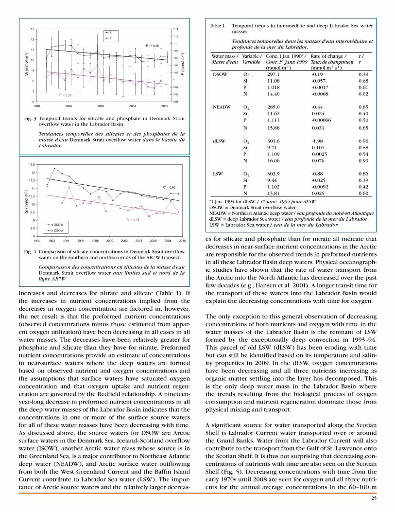
25

es for silicate and phosphate than for nitrate all indicate that decreases in near-surface nutrient concentrations in the Arctic are responsible for the observed trends in preformed nutrients in all these Labrador Basin deep waters. Physical oceanograph-ic studies have shown that the rate of water transport from the Arctic into the North Atlantic has decreased over the past few decades (e.g., Hansen et al. 2001). A longer transit time for the transport of these waters into the Labrador Basin would explain the decreasing concentrations with time for oxygen.

The only exception to this general observation of decreasing concentrations of both nutrients and oxygen with time in the water masses of the Labrador Basin is the remnant of LSW formed by the exceptionally deep convection in 1993–94. This parcel of old LSW (dLSW) has been eroding with time but can still be identified based on its temperature and salin-ity properties in 2009. In the dLSW, oxygen concentrations have been decreasing and all three nutrients increasing as organic matter settling into the layer has decomposed. This is the only deep water mass in the Labrador Basin where the trends resulting from the biological process of oxygen consumption and nutrient regeneration dominate those from physical mixing and transport.

A significant source for water transported along the Scotian Shelf is Labrador Current water transported over or around the Grand Banks. Water from the Labrador Current will also contribute to the transport from the Gulf of St. Lawrence onto the Scotian Shelf. It is thus not surprising that decreasing con-centrations of nutrients with time are also seen on the Scotian Shelf (Fig. 5). Decreasing concentrations with time from the early 1970s until 2008 are seen for oxygen and all three nutri-ents for the annual average concentrations in the 60–100 m

increases and decreases for nitrate and silicate (Table 1). If the increases in nutrient concentrations implied from the decreases in oxygen concentration are factored in, however, the net result is that the preformed nutrient concentrations (observed concentrations minus those estimated from appar-ent oxygen utilization) have been decreasing in all cases in all water masses. The decreases have been relatively greater for phosphate and silicate than they have for nitrate. Preformed nutrient concentrations provide an estimate of concentrations in near-surface waters where the deep waters are formed based on observed nutrient and oxygen concentrations and the assumptions that surface waters have saturated oxygen concentration and that oxygen uptake and nutrient regen-eration are governed by the Redfield relationship. A nineteen-year-long decrease in preformed nutrient concentrations in all the deep water masses of the Labrador Basin indicates that the concentrations in one or more of the surface source waters for all of these water masses have been decreasing with time. As discussed above, the source waters for DSOW are Arctic surface waters in the Denmark Sea. Iceland–Scotland overflow water (ISOW), another Arctic water mass whose source is in the Greenland Sea, is a major contributor to Northeast Atlantic deep water (NEADW), and Arctic surface water outflowing from both the West Greenland Current and the Baffin Island Current contribute to Labrador Sea water (LSW). The impor-tance of Arctic source waters and the relatively larger decreas-

Table 1 Temporal trends in intermediate and deep Labrador Sea water masses.

Tendances temporelles dans les masses d’eau intermédiaire et profonde de la mer du Labrador.

*1 Jan. 1994 for dLSW / 1er janv. 1994 pour dLSWDSOW = Denmark Strait overflow water NEADW = Northeast Atlantic deep water / eau profonde du nord-est AtlantiquedLSW = deep Labrador Sea water / eau profonde de la mer du LabradorLSW = Labrador Sea water / eau de la mer du Labrador

Water mass /Masse d’eau

Variable /Variable

Conc. 1 Jan. 1990* /Conc. 1er janv. 1990(mmol m-3 )

Rate of change /Taux de changement(mmol m-3 a-1 )

r /r

DSOW O2 297.1 -0.19 0.39Si 11.08 -0.057 0.68P 1.018 -0.0017 0.61N 14.40 -0.0008 0.02

NEADW O2 285.0 -0.44 0.85Si 11.62 0.024 0.40P 1.111 -0.00066 0.50

N 15.88 0.031 0.85

dLSW O2 301.6 -1.98 0.96Si 9.71 0.101 0.88P 1.109 0.0025 0.54N 16.06 0.076 0.90

LSW O2 303.9 -0.88 0.86Si 9.44 -0.025 0.39P 1.102 -0.0092 0.42N 15.81 0.025 0.60

Fig. 3 Temporal trends for silicate and phosphate in Denmark Strait overflow water in the Labrador Basin.

Tendances temporelles des silicates et des phosphates de la masse d’eau Denmark Strait overflow water dans le bassin du Labrador.

Si (

mm

ol m

-3)

P (m

mol

m-3)

Fig. 4 Comparison of silicate concentrations in Denmark Strait overflow water on the southern and northern ends of the AR7W transect.

Comparaison des concentrations en silicates de la masse d’eau Denmark Strait overflow water aux limites sud et nord de la ligne AR7W.

Si (

mm

ol m

-3)

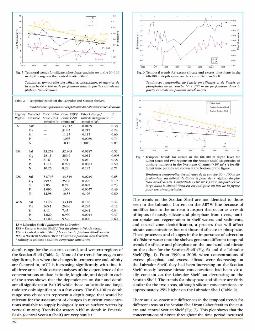
26

Fig. 5 Temporal trends for silicate, phosphate, and nitrate in the 60–100 m depth range on the central Scotian Shelf.

Tendances temporelles des silicates, phosphates, et nitrates de la couche 60 – 100 m de profondeur dans la partie centrale du plateau Néo-Écossais.

Si &

N (m

mol

m-3)

P (m

mol

m-3)

depth range for the eastern, central, and western regions of the Scotian Shelf (Table 2). None of the trends for oxygen are significant, but when the changes in temperature and salinity are factored in, AOU is increasing significantly with time in all three areas. Multivariate analyses of the dependence of the concentrations on date, latitude, longitude, and depth in each of the areas shows that the dependences on date and depth are all significant at P<0.05 while those on latitude and longi-tude are only significant in a few cases. The 60–100 m depth range was chosen to represent a depth range that would be relevant for the assessment of changes in nutrient concentra-tions available to supply biologically active surface waters by vertical mixing. Trends for waters >150 m depth in Emerald Basin (central Scotian Shelf) are very similar.

The trends on the Scotian Shelf are not identical to those seen in the Labrador Current on the AR7W line because of modifications to the nutrient transport that occur as a result of inputs of mostly silicate and phosphate from rivers, nutri-ent uptake and regeneration in shelf waters and sediments, and coastal zone denitrification, a process that will affect nitrate concentrations but not those of silicate or phosphate. These processes and changes in the importance of advection of offshore water onto the shelves generate different temporal trends for silicate and phosphate on the one hand and nitrate on the other for the Scotian Shelf (Fig. 6) and the Labrador Shelf (Fig. 1). From 1990 to 2008, when concentrations of excess phosphate and excess silicate were decreasing on the Labrador Shelf, they had been increasing on the Scotian Shelf, mostly because nitrate concentrations had been virtu-ally constant on the Labrador Shelf but decreasing on the Scotian Shelf. The trends for phosphate and silicate are fairly similar for the two areas, although silicate concentrations are approximately 25% higher on the Labrador Shelf (Table 2).

There are also systematic differences in the temporal trends for different areas on the Scotian Shelf from Cabot Strait to the east-ern and central Scotian Shelf (Fig. 7). This plot shows that the concentrations of nitrate throughout the time period increased

Fig. 7 Temporal trends for nitrate in the 60–100 m depth layer for Cabot Strait and two regions on the Scotian Shelf. Magnitudes of onshore transport in the Northeast Channel (×103 m3 s-1) for dif-ferent time periods are shown at the bottom of the figure.

Tendances temporelles des nitrates de la couche 60 – 100 m de profondeur au détroit de Cabot et pour deux régions du pla-teau Néo-Écossais. L’amplitude (×103 m3 s-1) du transport vers le large dans le chenal Nord-est est indiquée au bas de la figure pour certaines périodes.

N (m

mol

m-3)

Fig. 6 Temporal trends for excess silicate and excess phosphate in the 60–100 m depth range on the central Scotian Shelf.

Tendances temporelles de l’excès en silicates et de l’excès en phosphates de la couche 60 – 100 m de profondeur dans la partie centrale du plateau Néo-Écossais.

Si-N

(mm

ol m

-3)

P-N

/16

(mm

ol m

-3)

Region/Région

Variable/Variable

Conc. 1974/Conc. 1974(mmol m-3)*

Conc. 1990/Conc. 1990(mmol m-3)

Rate of change/Taux de changement(mmol m-3 a-1)

r/r

LS Sal* — 33.812 -0.0169 0.38O2 — 319.3 -0.217 0.24Si — 11.25 -0.115 0.66P — 1.066 -0.0080 0.74N — 10.12 0.004 0.07

ESS Sal 33.258 32.863 -0.0247 0.52O2 281.1 280.9 -0.012 0.003Si 8.16 7.41 -0.047 0.38P 1.114 0.997 -0.0073 0.50N 10.25 8.28 -0.123 0.71

CSS Sal 33.746 33.349 -0.0249 0.65O2 259.5 254.8 -0.297 0.19Si 9.85 8.74 -0.097 0.73P 1.096 1.006 -0.0057 0.49N 12.98 10.33 -0.166 0.80

WSS Sal 33.430 33.149 -0.176 0.44O2 265.1 260.6 -0.285 0.12Si 8.11 7.45 -0.042 0.34P 1.029 0.960 -0.0043 0.37N 11.09 9.52 -0.098 0.60

Table 2 Temporal trends on the Labrador and Scotian shelves.

Tendances temporelles sur les plateaux du Labrador et Néo-Écossais.

LS = Labrador Shelf / plateau du LabradorESS = Eastern Scotian Shelf / l’est du plateau Néo-ÉcossaisCSS = Central Scotian Shelf / le centre du plateau Néo-ÉcossaisWSS = Western Scotian Shelf / l’ouest du plateau Néo-Écossais* salinity is unitless / salinité s'exprime sans unité

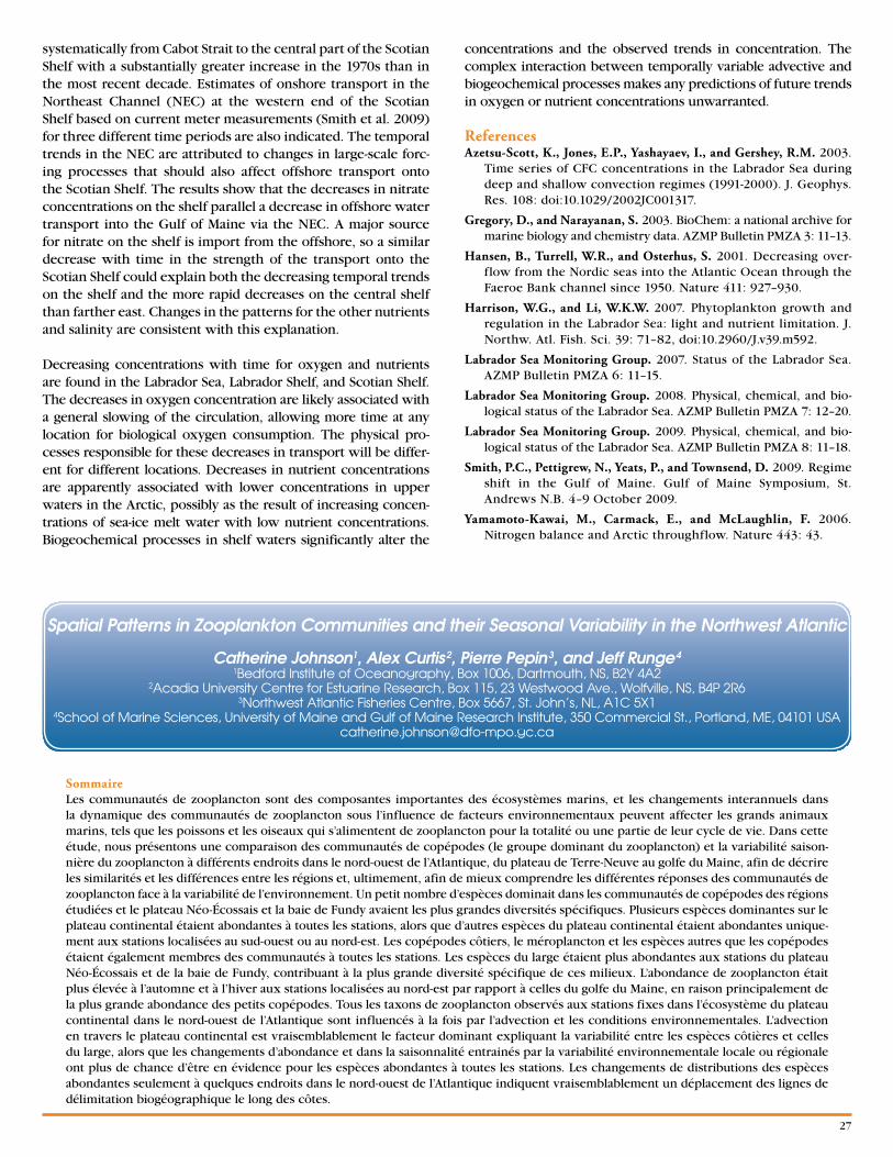
27

systematically from Cabot Strait to the central part of the Scotian Shelf with a substantially greater increase in the 1970s than in the most recent decade. Estimates of onshore transport in the Northeast Channel (NEC) at the western end of the Scotian Shelf based on current meter measurements (Smith et al. 2009) for three different time periods are also indicated. The temporal trends in the NEC are attributed to changes in large-scale forc-ing processes that should also affect offshore transport onto the Scotian Shelf. The results show that the decreases in nitrate concentrations on the shelf parallel a decrease in offshore water transport into the Gulf of Maine via the NEC. A major source for nitrate on the shelf is import from the offshore, so a similar decrease with time in the strength of the transport onto the Scotian Shelf could explain both the decreasing temporal trends on the shelf and the more rapid decreases on the central shelf than farther east. Changes in the patterns for the other nutrients and salinity are consistent with this explanation.

Decreasing concentrations with time for oxygen and nutrients are found in the Labrador Sea, Labrador Shelf, and Scotian Shelf. The decreases in oxygen concentration are likely associated with a general slowing of the circulation, allowing more time at any location for biological oxygen consumption. The physical pro-cesses responsible for these decreases in transport will be differ-ent for different locations. Decreases in nutrient concentrations are apparently associated with lower concentrations in upper waters in the Arctic, possibly as the result of increasing concen-trations of sea-ice melt water with low nutrient concentrations. Biogeochemical processes in shelf waters significantly alter the

concentrations and the observed trends in concentration. The complex interaction between temporally variable advective and biogeochemical processes makes any predictions of future trends in oxygen or nutrient concentrations unwarranted.

ReferencesAzetsu-Scott, K., Jones, E.P., Yashayaev, I., and Gershey, R.M. 2003.

Time series of CFC concentrations in the Labrador Sea during deep and shallow convection regimes (1991-2000). J. Geophys. Res. 108: doi:10.1029/2002JC001317.

Gregory, D., and Narayanan, S. 2003. BioChem: a national archive for marine biology and chemistry data. AZMP Bulletin PMZA 3: 11–13.

Hansen, B., Turrell, W.R., and Osterhus, S. 2001. Decreasing over-flow from the Nordic seas into the Atlantic Ocean through the Faeroe Bank channel since 1950. Nature 411: 927–930.

Harrison, W.G., and Li, W.K.W. 2007. Phytoplankton growth and regulation in the Labrador Sea: light and nutrient limitation. J. Northw. Atl. Fish. Sci. 39: 71–82, doi:10.2960/J.v39.m592.

Labrador Sea Monitoring Group. 2007. Status of the Labrador Sea. AZMP Bulletin PMZA 6: 11–15.

Labrador Sea Monitoring Group. 2008. Physical, chemical, and bio-logical status of the Labrador Sea. AZMP Bulletin PMZA 7: 12–20.

Labrador Sea Monitoring Group. 2009. Physical, chemical, and bio-logical status of the Labrador Sea. AZMP Bulletin PMZA 8: 11–18.

Smith, P.C., Pettigrew, N., Yeats, P., and Townsend, D. 2009. Regime shift in the Gulf of Maine. Gulf of Maine Symposium, St. Andrews N.B. 4–9 October 2009.

Yamamoto-Kawai, M., Carmack, E., and McLaughlin, F. 2006. Nitrogen balance and Arctic throughflow. Nature 443: 43.

SommaireLes communautés de zooplancton sont des composantes importantes des écosystèmes marins, et les changements interannuels dans la dynamique des communautés de zooplancton sous l’influence de facteurs environnementaux peuvent affecter les grands animaux marins, tels que les poissons et les oiseaux qui s’alimentent de zooplancton pour la totalité ou une partie de leur cycle de vie. Dans cette étude, nous présentons une comparaison des communautés de copépodes (le groupe dominant du zooplancton) et la variabilité saison-nière du zooplancton à différents endroits dans le nord-ouest de l’Atlantique, du plateau de Terre-Neuve au golfe du Maine, afin de décrire les similarités et les différences entre les régions et, ultimement, afin de mieux comprendre les différentes réponses des communautés de zooplancton face à la variabilité de l’environnement. Un petit nombre d’espèces dominait dans les communautés de copépodes des régions étudiées et le plateau Néo-Écossais et la baie de Fundy avaient les plus grandes diversités spécifiques. Plusieurs espèces dominantes sur le plateau continental étaient abondantes à toutes les stations, alors que d’autres espèces du plateau continental étaient abondantes unique-ment aux stations localisées au sud-ouest ou au nord-est. Les copépodes côtiers, le méroplancton et les espèces autres que les copépodes étaient également membres des communautés à toutes les stations. Les espèces du large étaient plus abondantes aux stations du plateau Néo-Écossais et de la baie de Fundy, contribuant à la plus grande diversité spécifique de ces milieux. L’abondance de zooplancton était plus élevée à l’automne et à l’hiver aux stations localisées au nord-est par rapport à celles du golfe du Maine, en raison principalement de la plus grande abondance des petits copépodes. Tous les taxons de zooplancton observés aux stations fixes dans l’écosystème du plateau continental dans le nord-ouest de l’Atlantique sont influencés à la fois par l’advection et les conditions environnementales. L’advection en travers le plateau continental est vraisemblablement le facteur dominant expliquant la variabilité entre les espèces côtières et celles du large, alors que les changements d’abondance et dans la saisonnalité entrainés par la variabilité environnementale locale ou régionale ont plus de chance d’être en évidence pour les espèces abondantes à toutes les stations. Les changements de distributions des espèces abondantes seulement à quelques endroits dans le nord-ouest de l’Atlantique indiquent vraisemblablement un déplacement des lignes de délimitation biogéographique le long des côtes.

Spatial Patterns in Zooplankton Communities and their Seasonal Variability in the Northwest Atlantic

Catherine Johnson1, Alex Curtis 2, Pierre Pepin 3, and Jeff Runge 41Bedford Institute of Oceanography, Box 1006, Dartmouth, NS, B2Y 4A2

2Acadia University Centre for Estuarine Research, Box 115, 23 Westwood Ave., Wolfville, NS, B4P 2R63Northwest Atlantic Fisheries Centre, Box 5667, St. John’s, NL, A1C 5X1

4School of Marine Sciences, University of Maine and Gulf of Maine Research Institute, 350 Commercial St., Portland, ME, 04101 USA catherine.johnson@dfo-mpo.gc.ca

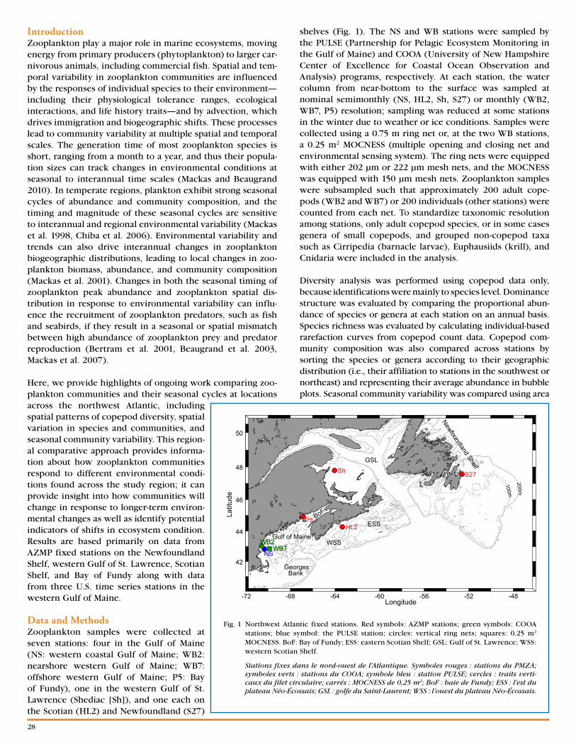
28

IntroductionZooplankton play a major role in marine ecosystems, moving energy from primary producers (phytoplankton) to larger car-nivorous animals, including commercial fish. Spatial and tem-poral variability in zooplankton communities are influenced by the responses of individual species to their environment—including their physiological tolerance ranges, ecological interactions, and life history traits—and by advection, which drives immigration and biogeographic shifts. These processes lead to community variability at multiple spatial and temporal scales. The generation time of most zooplankton species is short, ranging from a month to a year, and thus their popula-tion sizes can track changes in environmental conditions at seasonal to interannual time scales (Mackas and Beaugrand 2010). In temperate regions, plankton exhibit strong seasonal cycles of abundance and community composition, and the timing and magnitude of these seasonal cycles are sensitive to interannual and regional environmental variability (Mackas et al. 1998, Chiba et al. 2006). Environmental variability and trends can also drive interannual changes in zooplankton biogeographic distributions, leading to local changes in zoo-plankton biomass, abundance, and community composition (Mackas et al. 2001). Changes in both the seasonal timing of zooplankton peak abundance and zooplankton spatial dis-tribution in response to environmental variability can influ-ence the recruitment of zooplankton predators, such as fish and seabirds, if they result in a seasonal or spatial mismatch between high abundance of zooplankton prey and predator reproduction (Bertram et al. 2001, Beaugrand et al. 2003, Mackas et al. 2007).

Here, we provide highlights of ongoing work comparing zoo-plankton communities and their seasonal cycles at locations across the northwest Atlantic, including spatial patterns of copepod diversity, spatial variation in species and communities, and seasonal community variability. This region-al comparative approach provides informa-tion about how zooplankton communities respond to different environmental condi-tions found across the study region; it can provide insight into how communities will change in response to longer-term environ-mental changes as well as identify potential indicators of shifts in ecosystem condition. Results are based primarily on data from AZMP fixed stations on the Newfoundland Shelf, western Gulf of St. Lawrence, Scotian Shelf, and Bay of Fundy along with data from three U.S. time series stations in the western Gulf of Maine.

Data and MethodsZooplankton samples were collected at seven stations: four in the Gulf of Maine (NS: western coastal Gulf of Maine; WB2: nearshore western Gulf of Maine; WB7: offshore western Gulf of Maine; P5: Bay of Fundy), one in the western Gulf of St. Lawrence (Shediac [Sh]), and one each on the Scotian (HL2) and Newfoundland (S27)

shelves (Fig. 1). The NS and WB stations were sampled by the PULSE (Partnership for Pelagic Ecosystem Monitoring in the Gulf of Maine) and COOA (University of New Hampshire Center of Excellence for Coastal Ocean Observation and Analysis) programs, respectively. At each station, the water column from near-bottom to the surface was sampled at nominal semimonthly (NS, HL2, Sh, S27) or monthly (WB2, WB7, P5) resolution; sampling was reduced at some stations in the winter due to weather or ice conditions. Samples were collected using a 0.75 m ring net or, at the two WB stations, a 0.25 m2 MOCNESS (multiple opening and closing net and environmental sensing system). The ring nets were equipped with either 202 µm or 222 µm mesh nets, and the MOCNESS was equipped with 150 µm mesh nets. Zooplankton samples were subsampled such that approximately 200 adult cope-pods (WB2 and WB7) or 200 individuals (other stations) were counted from each net. To standardize taxonomic resolution among stations, only adult copepod species, or in some cases genera of small copepods, and grouped non-copepod taxa such as Cirripedia (barnacle larvae), Euphausiids (krill), and Cnidaria were included in the analysis.

Diversity analysis was performed using copepod data only, because identifications were mainly to species level. Dominance structure was evaluated by comparing the proportional abun-dance of species or genera at each station on an annual basis. Species richness was evaluated by calculating individual-based rarefaction curves from copepod count data. Copepod com-munity composition was also compared across stations by sorting the species or genera according to their geographic distribution (i.e., their affiliation to stations in the southwest or northeast) and representing their average abundance in bubble plots. Seasonal community variability was compared using area

Fig. 1 Northwest Atlantic fixed stations. Red symbols: AZMP stations; green symbols: COOA stations; blue symbol: the PULSE station; circles: vertical ring nets; squares: 0.25 m2 MOCNESS. BoF: Bay of Fundy; ESS: eastern Scotian Shelf; GSL: Gulf of St. Lawrence; WSS: western Scotian Shelf.

Stations fixes dans le nord-ouest de l’Atlantique. Symboles rouges : stations du PMZA; symboles verts : stations du COOA; symbole bleu : station PULSE; cercles : traits verti-caux du filet circulaire; carrés : MOCNESS de 0,25 m2; BoF : baie de Fundy; ESS : l’est du plateau Néo-Écossais; GSL : golfe du Saint-Laurent; WSS : l’ouest du plateau Néo-Écossais.

Longitude

Latit

ude

-72 -68 -64 -60 -56 -52 -48

42

44

46

48

50

HL2

NS

P5

S27Sh

WB2WB7

BoF

Gulf of Maine

GeorgesBank

WSS

ESS

Newfoundland Shelf

GSL

200m

100m

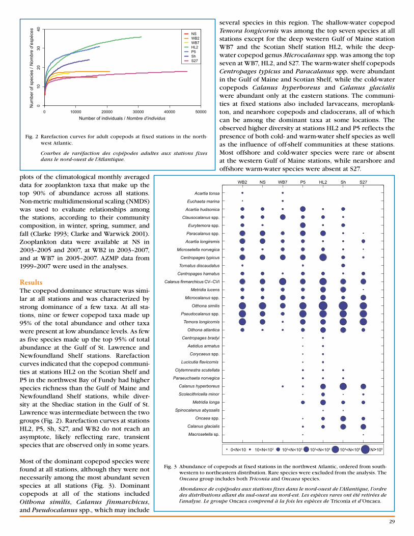
29

plots of the climatological monthly averaged data for zooplankton taxa that make up the top 90% of abundance across all stations. Non-metric multidimensional scaling (NMDS) was used to evaluate relationships among the stations, according to their community composition, in winter, spring, summer, and fall (Clarke 1993; Clarke and Warwick 2001). Zooplankton data were available at NS in 2003–2005 and 2007, at WB2 in 2003–2007, and at WB7 in 2005–2007. AZMP data from 1999–2007 were used in the analyses.

ResultsThe copepod dominance structure was simi-lar at all stations and was characterized by strong dominance of a few taxa. At all sta-tions, nine or fewer copepod taxa made up 95% of the total abundance and other taxa were present at low abundance levels. As few as five species made up the top 95% of total abundance at the Gulf of St. Lawrence and Newfoundland Shelf stations. Rarefaction curves indicated that the copepod communi-ties at stations HL2 on the Scotian Shelf and P5 in the northwest Bay of Fundy had higher species richness than the Gulf of Maine and Newfoundland Shelf stations, while diver-sity at the Shediac station in the Gulf of St. Lawrence was intermediate between the two groups (Fig. 2). Rarefaction curves at stations HL2, P5, Sh, S27, and WB2 do not reach an asymptote, likely reflecting rare, transient species that are observed only in some years.

Most of the dominant copepod species were found at all stations, although they were not necessarily among the most abundant seven species at all stations (Fig. 3). Dominant copepods at all of the stations included Oithona similis, Calanus finmarchicus, and Pseudocalanus spp., which may include

several species in this region. The shallow-water copepod Temora longicornis was among the top seven species at all stations except for the deep western Gulf of Maine station WB7 and the Scotian Shelf station HL2, while the deep-water copepod genus Microcalanus spp. was among the top seven at WB7, HL2, and S27. The warm-water shelf copepods Centropages typicus and Paracalanus spp. were abundant in the Gulf of Maine and Scotian Shelf, while the cold-water copepods Calanus hyperboreus and Calanus glacialis were abundant only at the eastern stations. The communi-ties at fixed stations also included larvaceans, meroplank-ton, and nearshore copepods and cladocerans, all of which can be among the dominant taxa at some locations. The observed higher diversity at stations HL2 and P5 reflects the presence of both cold- and warm-water shelf species as well as the influence of off-shelf communities at these stations. Most offshore and cold-water species were rare or absent at the western Gulf of Maine stations, while nearshore and offshore warm-water species were absent at S27.

Fig. 2 Rarefaction curves for adult copepods at fixed stations in the north-west Atlantic.

Courbes de raréfaction des copépodes adultes aux stations fixes dans le nord-ouest de l’Atlantique.

0 10000 20000 30000 40000 50000

010

2030

40

Number of individuals / Nombre d’individus

Num

ber o

f spe

cies

/ N

ombr

e d’

espè

ces

NSWB2WB7HL2P5ShS27

Fig. 3 Abundance of copepods at fixed stations in the northwest Atlantic, ordered from south-western to northeastern distribution. Rare species were excluded from the analysis. The Oncaea group includes both Triconia and Oncaea species.

Abondance de copépodes aux stations fixes dans le nord-ouest de l’Atlantique, l’ordre des distributions allant du sud-ouest au nord-est. Les espèces rares ont été retirées de l’analyse. Le groupe Oncaea comprend à la fois les espèces de Triconia et d’Oncaea.

WB2 NS WB7 P5 HL2 Sh S27

10<N<102 102<N<103 103<N<104 104<N<105

Acartia tonsa

Euchaeta marina

Acartia hudsonica

Clausocalanus spp.

Eurytemora spp.

Paracalanus spp.

Acartia longiremis

Microsetella norvegica

Centropages typicus

Tornatus discaudatus

Centropages hamatus

Calanus finmarchicus CV–CVI

Metridia lucens

Microcalanus spp.

Pseudocalanus spp.

Oithona similis

Temora longicornis

Oithona atlantica

Centropages bradyi

Aetidius armatus

Corycaeus spp.

Lucicutia flavicornis

Clytemnestra scutellata

Paraeuchaeta norvegica

Calanus hyperboreus

Scolecithricella minor

Metridia longa

Spinocalanus abyssalis

Oncaea spp.

Calanus glacialis

Macrosetella sp.

0<N<10 N>105

30

Climatological seasonal abundance cycles varied among sta-tions, and the timing of the seasonal abundance peak did not have a regionally coherent pattern. The climatological abundance peak was earliest at HL2 on the Scotian Shelf and latest at S27 on the Newfoundland Shelf and at the coastal western Gulf of Maine stations. On the other hand, the fall–winter abundance of zooplankton did have a spa-tially coherent pattern. It remained high at the three eastern stations, i.e., on the Newfoundland Shelf, on the Scotian Shelf, and in the Gulf of St. Lawrence (fall only; Sh was not sampled in winter due to ice), while it was low at the Gulf of Maine stations (representative seasonal cycles at HL2 and P5 are shown in Fig. 4). This pattern reflected differences primarily in the abundance of the small copepods O. similis,

Pseudocalanus spp., and T. longicornis between the two groups of stations (wintertime differences shown in Fig. 5; a similar pattern was observed in fall).

DiscussionThe northwest Atlantic continental shelf system is charac-terized by mean current flow toward the southwest and by extensive mixing of water masses and zooplankton commu-nities. Strong circulation and open boundaries contribute to the very large spatial ranges of marine zooplankton species in continental shelf systems. Zooplankton population and community dynamics are influenced by both advection and by local environmental conditions. Monitoring performed by AZMP and similar programs in the U.S. provides a unique

opportunity to compare seasonal and spatial zooplank-ton community patterns across a broad range of the northwest Atlantic using samples collected with the same or similar methodologies. The identification of large-scale spatial and seasonal zooplankton community patterns is necessary to interpret interannual changes in zooplankton communities observed on a local scale.

Despite the large size of the study area, several copepod species that had been previously characterized as core Scotian Shelf species (Tremblay and Roff 1983) were abundant at all stations. These species are likely to play the same roles in the ecosystem and respond similarly to variability in environmental conditions across their range, indicating a broad similarity in the core shelf zooplankton community across this part of the north-west Atlantic. Nevertheless, these similarities do not preclude spatial gradients in the abundance and sea-sonal dynamics of dominant species across the region that are driven by the species’ responses to their local environmental conditions, which are in turn influenced both by ocean circulation and by processes such as heat transfer between the ocean and atmosphere, freshwa-ter runoff, precipitation, and local mixing (Petrie et al. 2009) as well as interactions with other zooplankton.

Scotian Shelf (HL2) /Plateau Néo-Écossais

Bay of Fundy (P5) /Baie de Fundy

Others / autresMicrocalanus spp.Calanus hyperboreus

Paracalanus spp.

CirripediaCladocera

EuphausiaceaCentropages typicusAppendicularia Calanus finmarchicus CV−CVIBivalviaTemora longicornisCalanus finmarchicus CI−CIVPseudocalanus spp.Oithona similis

J F M A M J J A S O N D J F M A M J J A S O N DMonth / Mois Month / Mois

Abu

ndan

ce /

Abo

ndan

ce (i

nd m

-2)

x 105

4.0

3.5

3.0

2.5

2.0

1.5

1.0

0.5

0

Transform: Square root

50%

2005 20042005 2006

2007

2003

20042005

2006

2007

2005

2003

2004

20052003

2004

20052007

2D Stress: 0.0920072003

2004

2006

S27H2P5WB2WB7NS

Station

Bray-Curtis SimilarityWinter / Hiver

Fig. 5 Non-metric multidimensional scaling ordination of stations sampled in winter.

Ordination par cadrage multidimensionnel non-métrique des stations échantillonnées en hiver.

Fig. 4 Seasonal zooplankton variability on the Scotian Shelf and Bay of Fundy.

Variabilité saisonnière du zooplankton sur le plateau Néo-Écossais et dans la baie de Fundy.

31

For example, while O. similis, Pseudocalanus spp., and T. longicornis were abundant at all the stations examined, there was a coherent difference in their fall and winter abundance between the Gulf of Maine and the upstream, northeastern region. This spatial gradient in the seasonal dynamics of small copepods helps to explain the zooplankton community shift observed in the Gulf of Maine and on Georges Bank in the 1990s, which was characterized by high copepod diversity and dominance of small copepods (Pershing et al. 2005, Kane 2007). The 1990s community shift was associated with lower salinities and was hypothesized to be driven by increased advection from the Scotian Shelf or increased fall–winter pri-mary production related to stronger stratification (Pershing et al. 2005, Kane 2007). The spatially coherent pattern of high fall–winter zooplankton abundance upstream of the Gulf of Maine observed here in data collected primarily in the 2000s supports the hypothesis that the Gulf of Maine community shift of the 1990s was driven by increased advection from the Scotian Shelf. The zooplankton community shift of the 1990s appears to have favoured recruitment in some fish stocks (e.g., haddock) but not others (e.g., cod) (Mountain and Kane 2010).

The comparison of zooplankton communities across northwest Atlantic shelf stations also identified continental shelf copepod species that exhibit strong alongshore spatial abundance gradi-ents across the NW Atlantic shelf system, including C. typicus, Paracalanus spp., C. hyperboreus, and C. glacialis. These species are likely to be more sensitive indicators of interannual alongshore biogeographic shifts than species that are domi-nant throughout the region. For example, populations of C. hyperboreus and C. glacialis are maintained by flow from the Gulf of St. Lawrence onto the eastern Scotian Shelf, and their abundance on the Scotian Shelf is likely related to variation in outflow from the Gulf (Sameoto and Herman 1992).

In addition to core shelf species, the communities at the fixed stations include immigrants from nearshore and warm and cold offshore communities. The high species numbers observed on the Scotian Shelf and in Bay of Fundy stations, where species associations and water mass affiliations have been identified in several previous studies (Corey and Milne 1987, Tremblay and Roff 1983, Johnson and Petrie unpubl.), reflect the influence of all of these communities. At stations where these immigrant communities are found, species associated with nearshore environments such as bays and estuaries (e.g., Acartia spe-cies, Tortanus discaudatus, Eurytemora spp.) or with off-shore waters (e.g., Oithona atlantica, Scolecithricella minor, Aetidius armatus) are indicators of cross-shelf advection and mixing. At stations where these communities are currently absent, their appearance in the future may serve as an indicator of changes in water circulation patterns.

Identification of large-scale spatial and seasonal patterns through a regional comparison of zooplankton communities is necessary for interpreting zooplankton interannual variability within the regions. The patterns identified here have contributed to the development of zooplankton biogeographic and key species indi-cators, which will be used to evaluate whether zooplankton com-munities exhibit coherent interannual variation across the north-west Atlantic region and how regional, seasonal, and interannual environmental variability influences zooplankton communities.

AcknowledgementsThe authors acknowledge Chris Manning and the University of New Hampshire’s COOA program, Rebecca Jones and the PULSE Project, Fisheries and Oceans Canada’s Atlantic Zone Monitoring Program, and all the personnel who over the years have been involved with the sampling, collection, processing, and maintenance of these large databases for pro-viding data. We also thank Benoit Casault and Chris Manning for assistance with data analysis and Erica Head for useful discussions.

ReferencesBeaugrand, G., Brander, K.M., Lindley, J.A., Souissi, S., and Reid,

P.C. 2003. Plankton effect on cod recruitment in the North Sea. Nature 426: 661–664.

Bertram, D.F., Mackas, D.L., and McKinnell, S. 2001. The seasonal cycle revisited: interannual variation and ecosystem conse-quences. Prog. Oceanogr. 49: 283–307.

Chiba, S., Tadokoro, K., Sugisaki, H., and Saino, T. 2006. Effects of decadal climate change on zooplankton over the last 50 years in the western subarctic North Pacific. Glob. Change Biol. 12: 907–920.

Clarke, K.R. 1993. Non-parametric multivariate analyses of changes in community structure. Aust. J. Ecol. 18: 117–143.

Clarke, K.R., and Warwick, R.M. 2001. Change in marine communi-ties: an approach to statistical analysis and interpretation, 2nd

Edition. PRIMER-E, Plymouth, U.K.

Corey, S., and Milne, W.R. 1987. Recurrent groups of zooplankton in the Bay of Fundy and southwest Nova Scotia regions, Canada. Can. J. Zool. 65: 2400–2405.

Kane, J. 2007. Zooplankton abundance trends on Georges Bank, 1977–2004. ICES J. Mar. Sci. 64: 909–919.

Mackas, D.L., and Beaugrand, G. 2010. Comparisons of zooplank-ton time series. J. Mar. Syst. 79: 286–304.

Mackas, D.L. Goldblatt, R., and Lewis, A.G. 1998. Interdecadal variation in developmental timing of Neocalanus plumchrus populations at Ocean Station P in the subarctic North Pacific. Can. J. Fish. Aquat. Sci. 55: 1878–1893.

Mackas, D., Thomson, R.E., and Galbraith, M. 2001. Covariation of zooplankton community changes and oceanographic condi-tions on the British Columbia continental margin, 1995-1998. Can. J. Fish. Aquat. Sci. 58: 1–18.

Mackas, D.L., Batten, S., and Trudel, M. 2007. Effects on zooplank-ton of a warmer ocean: Recent evidence from the Northeast Pacific. Prog. Oceanogr. 75(2): 223–252.

Mountain, D.G., and Kane, J. 2010. Major changes in the Georges Bank ecosystem, 1980s to the 1990s. Mar. Ecol. Prog. Ser. 398: 81–91.

Pershing, A.J., Greene, C.H., Jossi, J.W., O'Brien, L., Brodziak, J.K.T., and Bailey, B.A. 2005. Interdecadal variability in the Gulf of Maine zooplankton community, with potential impacts on fish recruitment. ICES J. Mar. Sci. 62: 1511–1523.

Petrie, B., Pettipas, R.G., Petrie, W.M., and Soukhovtsev, V.V. 2009. Physical oceanographic conditions on the Scotian Shelf and in the Gulf of Maine during 2008. CSAS Res. Doc. 2009/039, 17 pp.

Sameoto, D.D., and Herman, A.W. 1992. Effect of the outflow from the Gulf of St. Lawrence on Nova Scotia Shelf zooplankton. Can. J. Fish. Aquat. Sci. 49: 857–869.

Tremblay, M.J., and Roff, J.C. 1983. Community gradients on the Scotian Shelf. Can. J. Fish. Aquat. Sci. 40: 598–661.

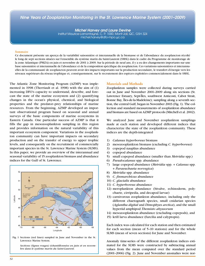
32

The Atlantic Zone Monitoring Program (AZMP) was imple-mented in 1998 (Therriault et al. 1998) with the aim of (1) increasing DFO’s capacity to understand, describe, and fore-cast the state of the marine ecosystem and (2) quantifying changes in the ocean’s physical, chemical, and biological properties and the predator–prey relationships of marine resources. From the beginning, AZMP developed an impor-tant observational program based on seasonal and annual surveys of the basic components of marine ecosystems in Eastern Canada. One particular success of AZMP is that it fills the gap in mesozooplankton sampling in this region and provides information on the natural variability of this important ecosystem component. Variations in the zooplank-ton community can have important impacts on secondary production and on the transfer of energy to upper trophic levels, and consequently on the recruitment of commercially important species in the St. Lawrence Marine System (SLMS). In this paper, we provide an overview of the interannual and seasonal variability of 15 zooplankton biomass and abundance indices for the Gulf of St. Lawrence.

Materials and MethodsZooplankton samples were collected during surveys carried out in June and November 2001–2009 along six sections (St. Lawrence Estuary, Sept-Îles, southwest Anticosti, Cabot Strait, Bonne Bay, Îles-de-la-Madeleine); sampling along a seventh sec-tion, the central Gulf, began in November 2003 (Fig. 1). The col-lection and standard measurements of zooplankton abundance and biomass are based on AZMP protocols (Mitchell et al. 2002).

We analyzed June and November zooplankton samplings made at each station and developed different indices that characterize the state of the zooplankton community. These indices are the depth-integrated

1) Calanus hyperboreus biomass 2) mesozooplankton biomass (excluding C. hyperboreus) 3) copepod nauplius abundance 4) copepod abundance 5) small copepod abundance (smaller than Metridia spp.) 6) Pseudocalanus spp. abundance 7) large copepod abundance (Metridia spp. + Calanus spp.

+ Paraeuchaeta norvegica) 8) Metridia spp. abundance 9) C. finmarchicus abundance 10) C. glacialis abundance 11) C. hyperboreus abundance 12) meroplankton abundance (bivalve, echinoderm, poly-

chaete, cirripedia, and decapod larvae) 13) carnivorous zooplankton abundance, including only the

different chaetognath species, small cnidarian species (Aglantha digital and Dimophyes arctica), and the small hyperiid amphipod Themisto abyssorum

14) mesozooplankton abundance (excluding copepods), and 15) krill larva abundance (furcilia and calyptopis).

Each index was calculated for each station and then estimated for each section (mean of 5–10 stations) and for the whole SLMS (mean of seven sections) for June and November.

Anomaly time-series of the different zooplankton indices esti-mated for the SLMS were constructed by subtracting annual values from the mean computed over the standard period (2001–2006) (Fig. 2). June and November anomalies were nor-

SommaireCe document présente un aperçu de la variabilité saisonnière et interannuelle de la biomasse et de l’abondance du zooplancton récolté le long de sept sections situées sur l’ensemble du système marin du Saint-Laurent (SMSL) dans le cadre du Programme de monitorage de la zone Atlantique (PMZA) en juin et novembre de 2001 à 2009. Sur la période de neuf ans, il y a eu des changements importants sur une base saisonnière et interannuelle de l’abondance et de la composition spécifique du zooplancton. Ces variations saisonnières et interannu-elles de la communauté de zooplancton peuvent avoir des impacts importants sur la production secondaire, le transfert d’énergie vers les niveaux supérieurs du réseau trophique et, conséquemment, sur le recrutement des espèces exploitées commercialement dans le SMSL.

Nine Years of Zooplankton Monitoring in the St . Lawrence Marine System (2001–2009)

Michel Harvey and Laure Devine Institut Maurice-Lamontagne, C. P. 1000, Mont-Joli, QC, G5H 3Z4

michel.harvey@dfo-mpo.gc.ca

-70 -68 -66 -64 -62 -60 -5846

47

48

49

50

51

52

0 100

km

.

N

Rimouski

Gaspé

St. LawrenceEstuary Line(TESL)

Sept-ÎlesLine (TSI)

AnticostiLine (TASO)

CentreLine (TCEN)

Îles-de-la-MadeleineLine (TIDM)

CabotStraitLine (TDC)

Bonne BayLine (TBB)

Longitude

edutitaL

0 100 200 +

m

Fig. 1 Sections (red lines) sampled in June and November in the St. Lawrence Marine System.

Sections (lignes rouges) échantillonnées en juin et en novem-bre dans le système marin du Saint-Laurent.

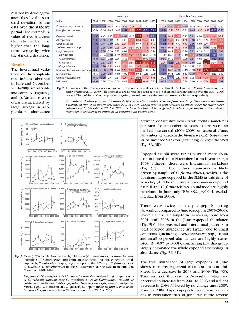
33

malized by dividing the anomalies by the stan-dard deviation of the data over the standard period. For example, a value of two indicates that the index was higher than the long-term average by twice the standard deviation.

ResultsThe interannual varia-tions of the zooplank-ton indices obtained in June and November 2001–2009 are variable and complex (Figures 3 and 4). Variations were often characterized by large swings in zoo-plankton abundance

between consecutive years while trends sometimes persisted for a number of years. There were no marked interannual (2001–2009) or seasonal (June, November) changes in the biomasses of C. hyperbore-us or mesozooplankton (excluding C. hyperboreus) (Fig. 3A, 3B).

Copepod nauplii were typically much more abun-dant in June than in November for each year except 2009, although there were interannual variations (Fig. 3C). The higher June abundance is likely driven by nauplii of C. finmarchicus, which is the dominant large copepod in the SLMS at this time of year (Fig. 3I). The interannual variations in copepod nauplii and C. finmarchicus abundance are highly correlated in June only (R2=0.82, p<0.001, exclud-ing data from 2006).

There were twice as many copepods during November compared to June (except in 2005–2006). Overall, there is a long-term increasing trend from 2001 until 2008 in the June copepod abundance (Fig. 3D). The seasonal and interannual patterns in total copepod abundance are largely due to small copepods (including Pseudocalanus spp.) (total and small copepod abundances are highly corre-lated; R2=0.97, p<0.001), confirming that this group largely dominated the whole copepod assemblage in abundance (Fig. 3E, 3F).

The total abundance of large copepods in June shows an increasing trend from 2001 to 2007 fol-lowed by a decrease in 2008 and 2009 (Fig. 3G). This was not the case in November, when we observed an increase from 2001 to 2003 and a slight decrease in 2004 followed by no change until 2009. Prior to 2004, large copepods were more numer-ous in November than in June, while the reverse

Index 2001 2002 2003 2004 2005 2006 2007 2008 2009 2001 2002 2003 2004 2005 2006 2007 2008 2009

C. hyperboreus biomass -1.38 -1.19 0.77 0.45 0.68 0.67 0.55 0.22 0.27 0.56 -0.67 1.79 -0.84 -0.38 -0.45 0.14 0.78 -0.37Mesoplankton biomass -0.16 -0.14 -0.02 0.03 -1.42 1.71 5.63 -2.81 -5.72 -1.44 0.75 0.81 -0.21 -0.86 0.95 0.98 -2.86 -0.72

Copepod nauplii -1.05 0.06 0.45 1.66 -0.94 -0.17 3.35 1.25 -1.81 -1.14 0.82 1.54 -0.12 -0.61 -0.50 1.45 1.40 0.52All copepods -1.06 -0.70 -0.52 0.16 0.41 1.71 0.84 1.45 0.38 -1.31 1.30 0.35 0.74 -0.96 -0.11 0.15 1.32 1.66Small copepods -1.05 -0.71 -0.59 0.13 0.58 1.64 0.47 1.44 0.55 -1.24 1.34 0.09 0.86 -0.96 -0.08 0.10 1.57 1.93 - Pseudocalanus spp. -1.16 -0.98 -0.54 0.96 0.76 0.95 0.38 1.44 0.94 -0.87 0.53 0.85 0.87 -1.57 0.19 -0.91 -0.42 2.01Large copepods -1.04 -0.65 -0.29 0.25 -0.09 1.83 1.85 1.10 -0.14 -1.08 0.42 1.79 -0.38 -0.52 -0.23 0.42 -1.11 -0.83 - Metridia spp. -1.17 -0.04 -0.98 -0.12 1.09 1.22 1.13 0.37 -0.33 0.22 0.46 -0.95 -0.49 1.67 -0.90 -0.54 -2.06 -0.80 - C. finmarchicus -0.84 -0.57 -0.32 0.31 -0.46 1.89 1.56 0.95 -0.64 -0.95 0.49 1.72 -0.30 -0.91 -0.06 0.23 -1.05 -1.12 - C. glacialis -0.72 -0.57 -0.91 -0.11 1.73 0.58 4.15 2.10 2.76 0.94 -1.26 -0.57 1.31 -0.65 0.23 3.21 0.39 1.12 - C. hyperboreus -1.43 -0.89 0.74 -0.08 1.18 0.48 1.47 1.01 2.25 -1.22 -0.66 1.73 -0.12 0.18 0.10 1.01 2.02 2.24Mesozooplankton (no copepods) -0.86 -0.66 -0.59 -0.44 1.15 1.40 2.42 -0.17 -0.14 -1.29 0.83 -0.70 -0.19 -0.10 1.45 4.14 7.62 3.25Meroplankton -0.49 -0.56 -0.51 -0.39 -0.05 2.01 0.14 -0.10 -0.08 -1.07 0.34 -0.40 0.22 -0.79 1.70 1.47 -0.22 -0.13Carnivorus zooplankton -0.80 -1.25 -0.47 0.31 1.00 1.21 0.98 1.10 0.58 -0.29 -1.50 -0.33 0.63 0.03 1.46 1.15 1.58 1.38Krill larvae -0.91 -0.25 -0.38 0.04 -0.44 1.94 4.27 0.97 -0.22 -0.75 -0.74 1.95 -0.24 -0.09 -0.14 0.90 2.16 -0.68

June / juin November / novembre

B: mesozooplankton biomass(excluding )C. hyperboreus

2000 2002 2004 2006 2008 20100

20

40

60

80

C: copepod nauplius abundance

02000 2002 2004 2006 2008 2010

5000

10000

15000

20000

25000

30000

2000 2002 2004 2006 2008 20100

10000

20000

30000

40000

50000 F: spp. abundancePseudocalanus

2000 2002 2004 2006 2008 20100

50000

100000

150000

200000

250000

300000 D: copepod abundance

2000 2002 2004 2006 2008 20100

50000

100000

150000

200000

250000

300000 E: small copepod abundance(smaller than spp.)Metridia

2000 2002 2004 2006 2008 20100

20000

40000

60000

80000

100000 G: large copepod abundance

)+Metridia spp. + Calanus spp.Paraeuchaeta norvegica

2000 2002 2004 2006 2008 20100

2000

4000

6000

8000

10000

12000

14000 H: spp. abundanceMetridia

2000 2002 2004 2006 2008 20100

20000

40000

60000

80000 I: abundanceC. finmarchicus

2000 2002 2004 2006 2008 20100

2000

4000

6000

8000 J: abundanceC. glacialis

2000 2002 2004 2006 2008 20100

5000

10000

15000

20000

25000 K: abundanceC. hyperboreus

g w

w( sssamoi

B· m

-2)

m-2)

· dni( ecnadnubA

m-2)

· dni( ecnadnubA

m-2)

· dni( ecnadnubA

A: Calanus hyperboreus biomass

2000 2002 2004 2006 2008 20100

20

40

60

80

100

JuneNovember

Fig. 3 Mean (±SD) zooplankton wet weight biomass (C. hyperboreus, mesozooplankton excluding C. hyperboreus) and abundance (copepod nauplii, copepods, small copepods, Pseudocalanus spp., large copepods, Metridia spp., C. finmarchicus, C. glacialis, C. hyperboreus) in the St. Lawrence Marine System in June and November 2001–2009.

Moyenne (± l’écart-type) de la biomasse humide de zooplancton (C. hyperboreus et de mésozooplancton sans C. hyperboreus) et de l’abondance (nauplii de copépodes, copépodes, petits copépodes, Pseudocalanus spp., grands copépodes, Metridia spp., C. finmarchicus, C. glacialis, C. hyperboreus) en juin et en novem-bre dans le système marin du Saint-Laurent entre 2001 et 2009.

Fig. 2 Anomalies of the 15 zooplankton biomass and abundance indices obtained for the St. Lawrence Marine System in June and November 2001–2009. The anomalies are normalized with respect to their standard deviations over the 2001–2006 period. Blue, white, and red represent negative, normal, and positive zooplankton conditions, respectively.

Anomalies calculées pour les 15 indices de biomasse et d’abondance de zooplancton du système marin du Saint-Laurent, en juin et en novembre, entre 2001 et 2009. Les anomalies sont réduites en divisant par les écarts-types calculés sur la période de 2001 à 2006. Le bleu, le blanc et le rouge représentent respectivement des valeurs négatives, normales et positives de la condition du zooplancton.

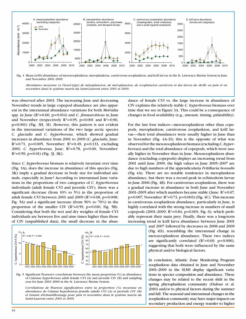
34

was observed after 2003. The increasing June and decreasing November trends in large copepod abundance are also appar-ent in the interannual abundance variations for both Metridia spp. in June (R2=0.60, p=0.014) and C. finmarchicus in June and November (respectively R2=0.95, p<0.001 and R2=0.96, p<0.001) (Fig. 3H, 3I). However, this pattern is not evident in the interannual variations of the two large arctic species C. glacialis and C. hyperboreus, which showed gradual increases in abundance from 2001 to 2009 (C. glacialis, June: R2=0.71, p=0.005, November: R2=0.49, p=0.133, excluding 2001; C. hyperboreus, June: R2=0.78, p=0.00, November: R2=0.59, p=0.01) (Fig. 3J, 3K).

Since C. hyperboreus biomass is relatively invariant over time (Fig. 3A), does the increase in abundance of this species (Fig. 3K) imply a gradual decrease in body size for individual ani-mals, especially in June? According to interannual June varia-tions in the proportions of two categories of C. hyperboreus individuals (adult female CVI and juvenile CIV), there was a significant decrease (from 10% to 5%) in the proportion of adult female CVI between 2001 and 2009 (R2=0.68, p=0.008; Fig. 5A) and a significant increase (from 50% to 70%) in the proportion of the smaller CIV (R2=0.59, p=0.016; Fig. 5B). Considering that both the wet and dry weights of female CVI individuals are between five and nine times higher than those of CIV (unpublished data), the small decrease in the abun-

dance of female CVI vs. the large increase in abundance of CIV explains the relatively stable C. hyperboreus biomass over time that we see in Figure 3A. This could be a consequence of changes in food availability (e.g., amount, timing, palatability).

For the last four indices—mesozooplankton other than cope-pods, meroplankton, carnivorous zooplankton, and krill lar-vae—their total abundances were usually higher in June than in November (Fig. 4A–D); this is the opposite of what was observed for the mesozooplankton biomass (excluding C. hyper-boreus) and the total abundance of copepods, which were usu-ally higher in November than in June. Mesozooplankton abun-dance (excluding copepods) displays an increasing trend from 2001 until June 2009; the high values in June 2005–2007 are due to high numbers of the appendicularia Fritillaria borealis (Fig 4A). There are no notable tendencies in meroplankton abundance, but there was a record peak in echinoderm larvae in June 2006 (Fig. 4B). For carnivorous zooplankton, there was a gradual increase in abundance in both June and November 2001–2005 after which numbers became stable (June: R2=0.67, p=0.007, November: R2=0.73, p=0.003) (Fig. 4C). This increase in carnivorous zooplankton abundance, particularly in June, is highly correlated with the strong increase in numbers of small copepods (2001–2009; R2=0.84, p<0.001; Fig. 6), which prob-ably represent their main prey. Finally, there was a long-term increasing trend in krill larva abundance between June 2001

and 2007 followed by decreases in 2008 and 2009 (Fig 4D), resembling the interannual change in mesozooplankton abundance. These two indices are significantly correlated (R2=0.69, p=0.006), suggesting that both were influenced by the same physical and/or biological factors.

In conclusion, Atlantic Zone Monitoring Program zooplankton data obtained in June and November 2001–2009 in the SLMS display significant varia-tions in species composition and abundance. These changes may be related to the recent shift in the spring phytoplankton community (Dufour et al. 2010) and/or to physical factors during the summer and fall. The seasonal and interannual changes in the zooplankton community may have major impacts on secondary production and energy transfer to higher

2000 2002 2004 2006 2008 20100

10000

20000

30000

40000

2000 2002 2004 2006 2008 20100

5000

15000

25000

35000

45000

2000 2002 2004 2006 2008 20100

2000

4000

6000

8000

m-2)

· dni( ecnadnubA

A: mesozooplankton abundance(excluding copepods)

B: meroplankton abundance(bivalve, echinoderm, polychaetecirripedia, and decapod larvae)

C: carnivorous zooplankton abundance(chaetognaths, small cnidarians,and a small hyperiid amphipod)

JuneNovember

2000 2002 2004 2006 2008 20100

500

1000

1500

2000

2500

3000

D: krill larva abundance(furcilia and calyptopis)

Fig. 4 Mean (±SD) abundance of mesozooplankton, meroplankton, carnivorous zooplankton, and krill larvae in the St. Lawrence Marine System in June and November 2001–2009.

Abondance moyenne (± l’écart-type) de mésoplancton, de méroplancton, de zooplancton carnivore et des larves de «krill» en juin et en novembre dans le système marin du Saint-Laurent entre 2001 et 2009.

R2= 0.68; P = 0.008

2001 2002 2003 2004 2005 2006 2007 2008 20090

5

10

15

A

C. h

yper

bore

us C

VI-f

(%)

R2= 0.59; P = 0.016

2001 2002 2003 2004 2005 2006 2007 2008 200920

30

40

50

60

70

80

90

100 B

C. h

yper

bore

us C

IV (%

)

Fig. 5 Significant Pearson’s correlations between the mean proportion (%) in abundance of Calanus hyperboreus adult female CVI (A) and juvenile CIV (B) and sampling year for June 2001–2009 in the St. Lawrence Marine System.

Corrélations de Pearson significatives entre la proportion (%) moyenne en abondance de Calanus hyperboreus femelle adulte CVI (A) et juvénile CIV (B) et l’année d’échantillonnage pour juin et novembre dans le système marin du Saint-Laurent entre 2001 et 2009.

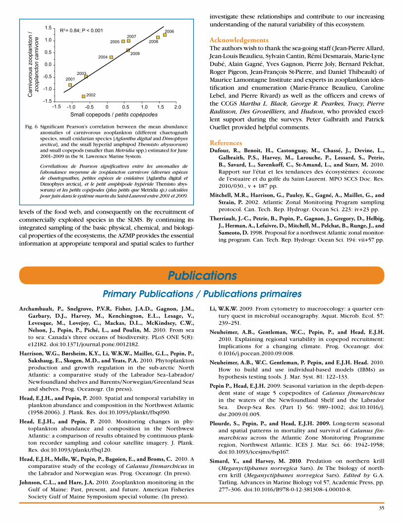
35

levels of the food web, and consequently on the recruitment of commercially exploited species in the SLMS. By continuing its integrated sampling of the basic physical, chemical, and biologi-cal properties of the ecosystems, the AZMP provides the essential information at appropriate temporal and spatial scales to further

investigate these relationships and contribute to our increasing understanding of the natural variability of this ecosystem.

AcknowledgementsThe authors wish to thank the sea-going staff (Jean-Pierre Allard, Jean-Louis Beaulieu, Sylvain Cantin, Rémi Desmarais, Marie-Lyne Dubé, Alain Gagné, Yves Gagnon, Pierre Joly, Bernard Pelchat, Roger Pigeon, Jean-François St-Pierre, and Daniel Thibeault) of Maurice Lamontagne Institute and experts in zooplankton iden-tification and enumeration (Marie-France Beaulieu, Caroline Lebel, and Pierre Rivard) as well as the officers and crews of the CCGS Martha L. Black, George R. Pearkes, Tracy, Pierre Radisson, Des Groseilliers, and Hudson, who provided excel-lent support during the surveys. Peter Galbraith and Patrick Ouellet provided helpful comments.

ReferencesDufour, R., Benoit, H., Castonguay, M., Chassé, J., Devine, L.,

Galbraith, P.S., Harvey, M., Larouche, P., Lessard, S., Petrie, B., Savard, L., Savenkoff, C., St-Amand, L., and Starr, M. 2010. Rapport sur l’état et les tendances des écosystèmes: écozone de l’estuaire et du golfe du Saint-Laurent. MPO SCCS Doc. Res. 2010/030., v + 187 pp.

Mitchell, M.R., Harrison, G., Pauley, K., Gagné, A., Maillet, G., and Strain, P. 2002. Atlantic Zonal Monitoring Program sampling protocol. Can. Tech. Rep. Hydrogr. Ocean Sci. 223: iv+23 pp.

Therriault, J.-C., Petrie, B., Pepin, P., Gagnon, J., Gregory, D., Helbig, J., Herman, A., Lefaivre, D., Mitchell, M., Pelchat, B., Runge, J., and Sameoto, D. 1998. Proposal for a northwest Atlantic zonal monitor-ing program. Can. Tech. Rep. Hydrogr. Ocean Sci. 194: vii+57 pp.

Technical Publications / Publications techniquesPublications

Archambault, P., Snelgrove, P.V.R, Fisher, J.A.D., Gagnon, J.M., Garbary, D.J., Harvey, M., Kenchington, E.L., Lesage, V., Levesque, M., Lovejoy, C., Mackas, D.L., McKindsey, C.W., Nelson, J., Pepin, P., Piché, L., and Poulin, M. 2010. From sea to sea: Canada’s three oceans of biodiversity. PLoS ONE 5(8): e12182. doi:10.1371/journal.pone.0012182.

Harrison, W.G., Børsheim, K.Y., Li, W.K.W., Maillet, G.L., Pepin, P., Sakshaug, E., Skogen, M.D., and Yeats, P.A. 2010. Phytoplankton production and growth regulation in the sub-arctic North Atlantic: a comparative study of the Labrador Sea–Labrador/Newfoundland shelves and Barents/Norwegian/Greenland Seas and shelves. Prog. Oceanogr. (In press).

Head, E.J.H., and Pepin, P. 2010. Spatial and temporal variability in plankton abundance and composition in the Northwest Atlantic (1958-2006). J. Plank. Res. doi:10.1093/plankt/fbq090.

Head, E.J.H., and Pepin, P. 2010. Monitoring changes in phy-toplankton abundance and composition in the Northwest Atlantic: a comparison of results obtained by continuous plank-ton recorder sampling and colour satellite imagery. J. Plank. Res. doi:10.1093/plankt/fbq120.

Head, E.J.H., Melle, W., Pepin, P., Bagøien, E., and Broms, C. 2010. A comparative study of the ecology of Calanus finmarchicus in the Labrador and Norwegian seas. Prog. Oceanogr. (In press).

Johnson, C.L., and Hare, J.A. 2010. Zooplankton monitoring in the Gulf of Maine: Past, present, and future. American Fisheries Society Gulf of Maine Symposium special volume. (In press).

Primary Publications / Publications primairesLi, W.K.W. 2009. From cytometry to macroecology: a quarter cen-

tury quest in microbial oceanography. Aquat. Microb. Ecol. 57: 239–251.

Neuheimer, A.B., Gentleman, W.C., Pepin, P., and Head, E.J.H. 2010. Explaining regional variability in copepod recruitment: Implications for a changing climate. Prog. Oceanogr. doi: 0.1016/j.pocean.2010.09.008.

Neuheimer, A.B., W.C. Gentleman, P. Pepin, and E.J.H. Head. 2010. How to build and use individual-based models (IBMs) as hypothesis testing tools. J. Mar. Syst. 81: 122–133.

Pepin P., Head, E.J.H. 2009. Seasonal variation in the depth-depen-dent state of stage 5 copepodites of Calanus finmarchicus in the waters of the Newfoundland Shelf and the Labrador Sea. Deep-Sea Res. (Part I) 56: 989–1002; doi:10.1016/j.dsr.2009.01.005.

Plourde, S., Pepin, P., and Head, E.J.H. 2009. Long-term seasonal and spatial patterns in mortality and survival of Calanus fin-marchicus across the Atlantic Zone Monitoring Programme region, Northwest Atlantic. ICES J. Mar. Sci. 66: 1942–1958; doi:10.1093/icesjms/fsp167.

Simard, Y., and Harvey, M. 2010. Predation on northern krill (Meganyctiphanes norvegica Sars). In The biology of north-ern krill (Meganyctiphanes norvegica Sars). Edited by G.A. Tarling. Advances in Marine Biology vol 57, Academic Press, pp. 277–306. doi:10.1016/B978-0-12-381308-4.00010-8.

-1.5 -0.5-1.0 0 0.5 1.0 1.5 2.0-1.5

-1.0

-0.5

0.0

0.5

1.0

1.5

2001

2002

2003

2004

2005

20062007

2008

2009

Small copepods / petits copépodes

R2= 0.84; P < 0.001C

arni

voro

us z

oopl

ankt

on /

zoop

lanc

ton

carn

ivor

e

Fig. 6 Significant Pearson’s correlation between the mean abundance anomalies of carnivorous zooplankton (different chaetognath species, small cnidarian species [Aglantha digital and Dimophyes arctica], and the small hyperiid amphipod Themisto abyssorum) and small copepods (smaller than Metridia spp.) estimated for June 2001–2009 in the St. Lawrence Marine System.

Corrélations de Pearson significatives entre les anomalies de l’abondance moyenne de zooplancton carnivore (diverses espèces de chaetognathes, petites espèces de cnidaires [Aglantha digital et Dimophyes arctica], et le petit amphipode hypéride Themisto abys-sorum) et les petits copépodes (plus petits que Metridia sp.) calculées pour juin dans le système marin du Saint-Laurent entre 2001 et 2009.

36

Technical Publications / Publications techniques

NAFO Research Document Series / Séries de Documents de recherche OPANO

Colbourne, E.B., Craig, J., Fitzpatrick, C., Senciall, D., Stead, P., and Bailey, W. 2009. An assessment of the physical oceanographic environment on the Newfoundland and Labrador Shelf in NAFO Subareas 2 and 3 during 2008. NAFO SCR Doc. 2009/17, Serial No. 5649, 20 pp.

Colbourne, E.B., Craig, J., Fitzpatrick, C., Senciall, D., Stead, P., and Bailey, W. 2010. An assessment of the physical oceanographic environment on the Newfoundland and Labrador Shelf in NAFO Subareas 2 and 3 during 2009. NAFO SCR Doc. 2010/16, Serial No. N5770, 25 pp.

Hendry, R.M. 2009. Environmental conditions in the Labrador Sea in 2008. NAFO SCR Doc. 2009/27, Serial No. N5662, 9 pp.

Maillet, G. 2010. Seasonality of phytoplankton abundance derived

Canadian Science Advisory Secretariat (CSAS) / Secrétariat canadien de consultation scientifique (SCCS)Research Documents / Documents de recherche

from satellite data in the northwest Atlantic during 1998 to 2009. NAFO SCR Doc. 2010/13, Serial No. N5766, 20 pp.

Petrie, B., and Pettipas, R.G. 2010. Physical oceanographic condi-tions on the Scotian Shelf and in the eastern Gulf o f Maine (NAFO areas 4V, W, X) during 2009. NAFO SCR Doc. 2010/12, Serial No. N5765, 22 pp.

Petrie, B., Pettipas, R.G., Petrie, W.M., and Soukhovtsev, V.V. 2009. Physical oceanographic conditions on the Scotian Shelf and in the eastern Gulf of Maine (NAFO areas 4V, W, X) during 2008. NAFO SCR Doc. 2009/15, Serial No. N5643, 20 pp.

Yashayaev, I., and Greenan, B.J.W. 2010. Environmental conditions in the Labrador Sea in 2009. NAFO SCR Doc. 2010/17, Serial No. N5771, 17 pp.

Chassé, J., and Pettipas, R.G. 2009. Temperature conditions in the southern Gulf of St. Lawrence during 2008 relevant to snow crab. DFO CSAS Res. Doc. 2009/087, 30 pp.

Colbourne, E.B., Craig, J., Fitzpatrick, C., Senciall, D., Stead, P. and Bailey, W. 2009. An assessment of the physical oceanographic environment on the Newfoundland and Labrador Shelf during 2008. DFO CSAS Res. Doc. 2009/032, 23 pp.

Dufour, R., Benoît, H., Castonguay, M., Chassé, J., Devine, L., Galbraith, P., Harvey, M., Larouche, P., Lessard, S., Petrie, B., Savard, L., Savenkoff, C., St-Amand, L., and Starr, M. 2010. Ecosystem status and trends report: Estuary and Gulf of St. Lawrence ecozone. DFO CSAS Res. Doc. 2010/030, 193 pp.

Galbraith, P.S., Pettipas, R.G., Chassé, J., Gilbert, D., Larouche, P., Pettigrew, B., Gosselin, A., Devine, L., and Lafleur, C. 2009. Physical oceanographic conditions in the Gulf of St. Lawrence in 2008. DFO CSAS Res. Doc. 2009/014, 73 pp.

Galbraith, P.S., Pettipas, R.G., Chassé, J., Gilbert, D., Larouche, P., Pettigrew, B., Gosselin, A., Devine, L., and Lafleur, C. 2010. Physical oceanographic conditions in the Gulf of St. Lawrence in 2009. DFO CSAS Res. Doc. 2010/035, 77 pp.

Harrison, G., Johnson, C., Head, E., Spry, J., Pauley, K., Maass, H., Kennedy, M., Porter, C., and Soukhovtsev, V. 2009. Optical, chemical, and biological oceanographic conditions in the Maritimes Region in 2008. DFO CSAS Res. Doc. 2009/054, 61 pp.

Harvey, M., and Devine, L. 2009. Oceanographic conditions in the Estuary and the Gulf of St. Lawrene during 2008: zooplankton. DFO CSAS Res. Doc. 2009/083, 60 pp.

Head, E., and Pepin, P. 2009. Long-term variability in phytoplank-ton and zooplankton abundance in the Northwest Atlantic in Continuous Plankton Recorder (CPR) samples. DFO CSAS Res. Doc. 2009/063, 35 pp.

Petrie, B., Pettipas, R.G., Petrie, W.M., and Soukovtsev. 2009. Physical oceanographic conditions on the Scotian Shelf and in the Gulf of Maine during 2008. DFO CSAS Res. Doc. 2009/039, 17 pp.

Petrie, B., Pettipas, R.G., and Petrie, W.M. 2009. An overview of meteorological, sea ice and sea-surface temperature conditions off Nova Scotia and the Gulf of Maine during 2008. DFO CSAS Res. Doc. 2009/041, 38 pp.

O’Brien, T.D., Lopez-Urrutia, A., Wiebe, P.H., and Hay, S. (Eds.). 2008. ICES Zooplankton Status Report 2006/2007. ICES Cooperative Research Report No. 292, 167 pp.

Others / Autres

DFO (Colbourne E.B.). 2009. 2008 State of the ocean: physical oceanographic conditions in the Newfoundland and Labrador Region. DFO CSAS Sci. Advis. Rep. 2009/057.

DFO (Galbraith, P.S.). 2009. State of the ocean 2008: physical oceanographic conditions in the Gulf of St. Lawrence. DFO CSAS Sci. Advis. Rep. 2009/019.

Science Advisory Reports / Avis scientifiques

DFO (Harrison, G., Johnson, C.). 2009. 2007 State of the ocean: chemical and biological oceanographic conditions in the Gulf of Maine - Bay of Fundy and on the Scotian Shelf. DFO CSAS Sci. Advis. Rep. Rep. 2009/005.

DFO (Harrison, G., Johnson, C.). 2009. 2008 State of the ocean: chemical and biological oceanographic conditions in the Gulf of Maine - Bay of Fundy and on the Scotian Shelf. DFO CSAS Sci.Advis. Rep. 2009/054.

(All advisory reports are available in English and French / Tous les rapports d’avis sont disponibles en français et en anglais)