ÉCOLE POLYTECHNIQUEPROMOTION X2008

Guilherme MAZANTI

Rapport de stage de recherche

Stabilisation des systèmes linéaires àexcitation persistante

Non confidentiel

Option : Mathématiques AppliquéesChamp de l’option : MAP593 - Automatique et Recherche OpérationnelleDirecteur de l’option : Yacine CHITOURDirecteurs de stage : Yacine CHITOUR et Mario SIGALOTTIDates du stage : 06/04/2011 à 24/06/2011Nom et adresse de l’organisme : École Polytechnique

CMAP - Centre de Mathématiques AppliquéesRoute de Saclay91128 PALAISEAU CEDEX, France

Abstract

We study the control system x = Ax + α(t)bu where the pair (A,b) is controllable,x ∈ Rd , u ∈ R is a scalar control and the unknown signal α : R+ → [0,1] is persistentlyexciting (PE), i.e., there exists T ≥ µ > 0 such that, for all t ∈ R+,

r t+Tt α(s)ds ≥ µ . We

are interested in the problem of stabilization at an arbitrary rate of convergence of thissystem by a linear state feedback u = −Kx. We start by recalling the main results alreadyobtained for this kind of system, and that stabilization at an arbitrary rate is not possible forgeneral PE signals when A is the double integrator. We thus restrict the class of PE signalsconsidered by taking only M-lipschitzian PE signals α . In this case, we can show that thedouble integrator can be stabilized at an arbitrary rate of convergence.

Résumé

On étudie le système de commande x=Ax+α(t)bu où la paire (A,b) est commandable,x∈Rd , u∈R est une commande scalaire et le signal inconnu α :R+→ [0,1] est à excitationpersistante (PE), i.e., il existe T ≥ µ > 0 tels que, pour tout t ∈ R+,

r t+Tt α(s)ds ≥ µ . On

s’intéresse au problème de stabilisation à taux de convergence arbitraire de ce système parun retour d’état linéaire u =−Kx. Nous commençons par rappeler les résultats principauxdéjà obtenus pour ce type de système, notamment que la stabilisation à taux de conver-gence arbitraire n’est pas possible pour des signaux PE généraux lorsque A est le doubleintégrateur. Nous restreignons ainsi la classe de signaux PE étudiée en ne considérant queles signaux PE M-lipschitziens α . Dans ce cas, on peut montrer que le double intégrateurpeut être stabilisé à un taux de convergence arbitraire.

Resumo

Estudamos o sistema de controle x = Ax+α(t)bu em que o par (A,b) é controlável,x∈Rd , u∈R é um controle escalar e o sinal desconhecido α :R+→ [0,1] é um sinal a exci-tação persistente (PE), i.e., existem T ≥ µ > 0 tais que, para todo t ∈R+,

r t+Tt α(s)ds≥ µ .

Interessamo-nos ao problema de estabilização a taxa de convergência arbitrária deste sis-tema através de uma realimentação de estado linear u = −Kx. Começamos retomando osprincipais resultados já obtidos para este tipo de sistema, em particular que a estabilizaçãoa velocidade arbitrária não é possível para sinais PE genéricos no caso em que A é o duplointegrador. Restringimos assim a classe de sinais PE estudada, considerando apenas os si-nais PE M-lipschitzianos α . Neste caso, pode-se mostrar que o duplo integrador pode serestabilizado a uma taxa de convergência arbitrária.

i

ii

Contents1 Introduction 1

1.1 Non-autonomous linear systems . . . . . . . . . . . . . . . . . . . . . . . . . 11.2 Control systems . . . . . . . . . . . . . . . . . . . . . . . . . . . . . . . . . . 11.3 Switched control systems . . . . . . . . . . . . . . . . . . . . . . . . . . . . . 21.4 Persistence of excitation . . . . . . . . . . . . . . . . . . . . . . . . . . . . . 31.5 Purpose of the project . . . . . . . . . . . . . . . . . . . . . . . . . . . . . . . 31.6 Organization of the document . . . . . . . . . . . . . . . . . . . . . . . . . . . 5

2 Notations and definitions 62.1 Basic definitions . . . . . . . . . . . . . . . . . . . . . . . . . . . . . . . . . . 62.2 PE and PEL signals and systems . . . . . . . . . . . . . . . . . . . . . . . . . 62.3 Controllability . . . . . . . . . . . . . . . . . . . . . . . . . . . . . . . . . . . 72.4 Stabilizability . . . . . . . . . . . . . . . . . . . . . . . . . . . . . . . . . . . 7

3 Previous results 93.1 Existence of a stabilizer . . . . . . . . . . . . . . . . . . . . . . . . . . . . . . 93.2 Stabilization at an arbitrary rate . . . . . . . . . . . . . . . . . . . . . . . . . . 10

4 Main result 124.1 Strategy of the proof . . . . . . . . . . . . . . . . . . . . . . . . . . . . . . . 134.2 Change of variables . . . . . . . . . . . . . . . . . . . . . . . . . . . . . . . . 134.3 Properties of the system in the new variables . . . . . . . . . . . . . . . . . . . 15

4.3.1 Polar coordinates . . . . . . . . . . . . . . . . . . . . . . . . . . . . . 154.3.2 Rotations around the origin . . . . . . . . . . . . . . . . . . . . . . . . 154.3.3 Decomposition of the time in intervals I+ and I0 . . . . . . . . . . . . 184.3.4 Estimations on intervals I+ . . . . . . . . . . . . . . . . . . . . . . . . 194.3.5 Estimations on intervals I0 . . . . . . . . . . . . . . . . . . . . . . . . 234.3.6 Estimate of y . . . . . . . . . . . . . . . . . . . . . . . . . . . . . . . 35

4.4 Proof of Theorem 4.1 . . . . . . . . . . . . . . . . . . . . . . . . . . . . . . . 35

5 Conclusion 37

References 38

iii

iv

1 IntroductionThe aim of the project was to continue the study of persistently excited (PE) linear controlsystems of [3, 4]. These systems can be written in the form

x = Ax+α(t)Bu

where x ∈ Rd , u ∈ Rm is the control and α : R+→ [0,1] is a scalar persistently exciting signal,that is, there exists two constants T , µ with T ≥ µ > 0 such that, for every t ∈ R+,

w t+T

tα(s)ds≥ µ.

Throughout this document, we shall consider only the case where the control u is scalar, andthus the matrix B is actually a column vector b ∈ Rd .

This project was developed as the research project in the end of the third year of academicstudies at École Polytechnique.

1.1 Non-autonomous linear systemsThe study of linear systems of differential equations has a great interest, from both applied andtheoretical points of view. These systems arise from linear models, as well as linearizations ofnon-linear systems at equilibrium points or along solutions. Consider a system in the form

x = A(t)x (1.1)

where x ∈ Rd and t 7→ A(t) is a bounded measurable application from a time interval I to theset of square d× d matrices with real coefficients, Md(R). When A is constant, the systemis called autonomous, and non-autonomous otherwise. By Carathéodory Theorem, given aninitial condition x(t0) = x0 for a certain t0 ∈ I, System (1.1) has a unique absolutely continuoussolution, defined over the whole interval I. We shall be interested in the case I = R+.

The most simple case of non-autonomous linear system is when A(t) may take only twovalues, A1 and A2, and another simple case is when A(t) takes its values on the convex envelopeof the set A1,A2, i.e., A(t) ∈ [A1,A2] = (1−α)A1 +αA2,α ∈ [0,1], A1 and A2 being twofixed matrices of Md(R). The system may hence be written in the form

x = ((1−α(t))A1 +α(t)A2)x (1.2)

with α(t) ∈ 0,1 or α(t) ∈ [0,1]. Such a system is thus able to switch between the dynamicsof A1 and A2.

1.2 Control systemsThe theory of linear autonomous control systems is concerned with the study of systems of theform

x = Ax+Bu

with x ∈Rd , u∈Rm, A∈Md(R) and B∈Md,m(R). The function u is the control of the system,which we choose trying to make the system have a certain prescribed behavior. A usual way tochoose this control is on the form of a linear state feedback u =−Kx with K ∈Mm,d(R). Thischoice corresponds to replacing the original dynamics of the non-controlled system, given bythe matrix A, with a new dynamics, given by the matrix A−BK.

1

1.3 Switched control systemsWe can now combine the idea of replacing the dynamics of a system given by a certain matrixA with a new controlled dynamics A−BK shown in Section 1.2 and the idea of a linear systemswitching between two dynamics as in (1.2): by taking A1 = A and A2 = A−BK on (1.2), weget

x = (A−α(t)BK)x

with α(t) ∈ [0,1]. More generally, we are interested in the switched control system

x = Ax+α(t)Bu. (1.3)

It is thus a system where the control u cannot act at every time t, but only when α(t) is active.System (1.3) is a linear switched control system and is the only case of switched control systemthat we shall study in this document; for a more complete reference, see, for instance, [6].

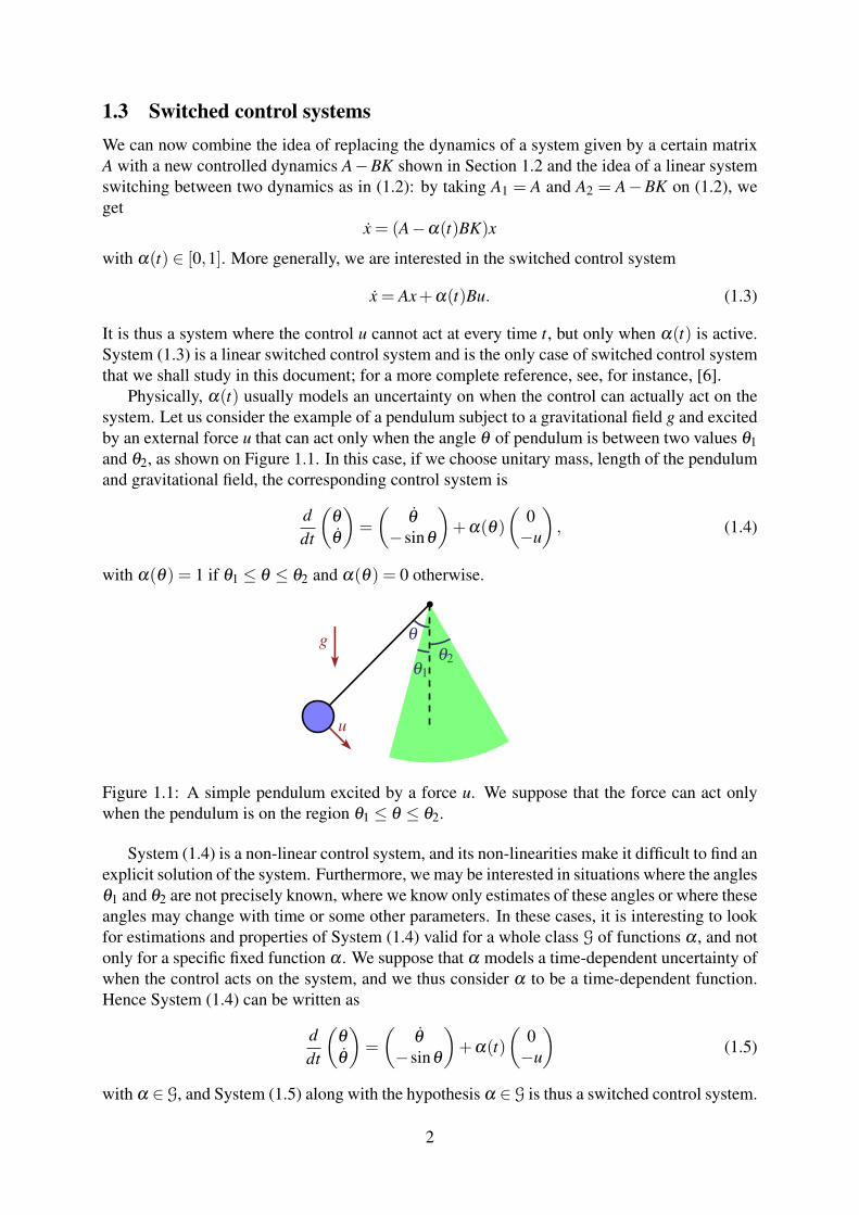
Physically, α(t) usually models an uncertainty on when the control can actually act on thesystem. Let us consider the example of a pendulum subject to a gravitational field g and excitedby an external force u that can act only when the angle θ of pendulum is between two values θ1and θ2, as shown on Figure 1.1. In this case, if we choose unitary mass, length of the pendulumand gravitational field, the corresponding control system is

ddt

(θ

θ

)=

(θ

−sinθ

)+α(θ)

(0−u

), (1.4)

with α(θ) = 1 if θ1 ≤ θ ≤ θ2 and α(θ) = 0 otherwise.

u

g θ

θ1θ2

Figure 1.1: A simple pendulum excited by a force u. We suppose that the force can act onlywhen the pendulum is on the region θ1 ≤ θ ≤ θ2.

System (1.4) is a non-linear control system, and its non-linearities make it difficult to find anexplicit solution of the system. Furthermore, we may be interested in situations where the anglesθ1 and θ2 are not precisely known, where we know only estimates of these angles or where theseangles may change with time or some other parameters. In these cases, it is interesting to lookfor estimations and properties of System (1.4) valid for a whole class G of functions α , and notonly for a specific fixed function α . We suppose that α models a time-dependent uncertainty ofwhen the control acts on the system, and we thus consider α to be a time-dependent function.Hence System (1.4) can be written as

ddt

(θ

θ

)=

(θ

−sinθ

)+α(t)

(0−u

)(1.5)

with α ∈ G, and System (1.5) along with the hypothesis α ∈ G is thus a switched control system.

2

1.4 Persistence of excitationIn the switched control system (1.3), the signal α determines when the control signal u mayact. We suppose that α is not precisely known, and the only information on α we have is thatit is chosen in a certain class of functions G. The question that arises is which kind of classof functions G may be natural and useful in practice. It is obviously not interesting to chooseG= L∞(R+, [0,1]) since this class contains the constant function equal to 0 and functions whichare arbitrarily small in norm L∞ or that are different from 0 only in a finite time interval, and, inthese cases, the control has a small or even null influence on the behavior of the non-controlledsystem x = Ax. We are thus looking for a class of functions that are “active” often enoughand that, at each activation, have a certain “minimum degree of activation”. For this purpose,[3, 4] use signals α satisfying a condition called persistent excitation (PE): given two positiveconstants T,µ with T ≥ µ , we say that a measurable function α : R+ → [0,1] is in the classG(T,µ) if, for every t ≥ 0, w t+T

tα(s)ds≥ µ. (1.6)

This condition is known as the condition of persistent excitation and appears naturally in thecontext of identification and adaptive control, as in [8]. Roughly speaking, it means that, forevery time interval of length T , the amount of time that α is “active” during this time windowis lower bounded by a positive constant.

1.5 Purpose of the projectThe research project aimed at answering an open question raised in [4], its Open Problem 5. Weconsider the problem of stabilization to the origin, by means of a linear state feedback u =−Kx,of the persistently excited control system

x = Ax+α(t)bu (1.7)

where x ∈ Rd , u ∈ R and α ∈ G(T,µ). We want this stabilization to be uniform with respectto the signal α: K may depend on T and µ , but it should not depend on a particular signalα ∈ G(T,µ).

One may think that, intuitively, the stabilization of a system as (1.7) is possible under reason-able hypothesis on (A,b), due to the condition (1.6) imposed on α . Indeed, if we suppose thatthe linear control system defined by (A,b) is stabilizable, meaning that there exists KT ∈Rd suchthat A−bK is Hurwitz, and if we suppose, in order to simplify the reasoning, that α(t)∈ 0,1,then, by choosing such a K, we can “stabilize” System (1.7) at least when α(t) = 1, which, dueto the condition (1.6) on α , happens at least for a total time µ on every time window of length T ,but this is not actually a stabilization of the system since we still have to deal with time intervalswhen α(t) = 0. We may then think that, if we know the behavior of the uncontrolled systemx = Ax, we can try to compensate any destabilization due to its dynamics when α(t) = 0 byastutely choosing K so that the stabilization provided by A−bK when α(t) = 1 will eventuallystabilize the system. This intuition can also be used in the case α(t) ∈ [0,1]: one can prove(see [4]) that it is possible, for every ρ > 0, to choose a K that stabilizes System (1.7) for everyα ∈ L∞(R+, [ρ,1]). Then, for System (1.7) with a general α ∈ G(T,µ), by choosing ρ smallenough, Equation (1.6) shows that we have α(t) ≥ ρ at least for a total time that is uniformlylower bounded on every time window of length T ; we have then “good” time intervals whereα is lower bounded by ρ and we know how to stabilize the system, and “bad” time intervalswhere α is smaller than ρ . We then expect that, by studying the behavior of the system in the

3

“bad” time intervals, we can choose K in order to compensate an eventual explosive behavior ofthe solution in the “bad” time intervals by convergence in the “good” ones in order to stabilizethe system.

This intuition was proved true in [4], where it is shown that stabilization to the origin ofSystem (1.7) is possible if (A,b) is a controllable pair and every eigenvalue of A has non-positivereal part (see the precise statement in Theorem 3.2 below).

Let us just say that, even if we mentioned above quite quickly the study of the behavior ofthe system in “bad” intervals, this is actually a difficult point. All the difficulty comes from thefact that we want to choose a feedback u = −Kx with K that is independent of α ∈ G(T,µ),and thus it is the same K that acts on both “good” and “bad” intervals. The feedback gain Kis chosen in such a way that the behavior on “good” intervals is known and controlled, but wenow nothing a priori on the effects of a particular choice of K on “bad” intervals, and obtainingestimates in this case is nontrivial, since the usual estimates, such as Gronwall’s Lemma, areusually not fine enough to provide a useful result.

We can now ask the question of stabilization at an arbitrary rate: we want to choose afeedback u =−Kx such that every solution of x = (A−α(t)bK)x converges to 0 exponentiallyat a rate which is faster than a prescribed constant λ . In the case of a linear control systemx = Ax+Bu, the question is then to study the eigenvalues of A−BK, and the answer is givenby the Pole Shifting Theorem, which guarantees that, for every controllable pair of matrices(A,B) ∈Md(R)×Md,m(R) and every unitary polynomial P of degree d with real coefficients,there exists K ∈Mm,d(R) such that P is the characteristic polynomial of A−BK, and then wecan arbitrarily choose the eigenvalues of A−BK.

In the case α(t) ∈ 0,1, one might think that stabilization at an arbitrary rate still holdstrue for a controllable pair (A,b): it would suffice to choose K such that the solution of x =(A− bK)x stabilizes the system fast enough and that its convergence rate compensates anypossible explosive behavior when α(t) = 0. But this intuition is shown to be false in [4], whereit is shown that, in dimension d = 2, there exists ρ? such that, if 0 < µ

T < ρ?, then the maximalrate of convergence of System (1.7) is finite, which means that there exists a constant C suchthat, for every KT ∈ R2, there exists a signal α ∈ G(T,µ) and an initial condition x0 of norm 1such that the corresponding solution x(t) of the system x = (A−αbK)x satisfies

limsupt→+∞

log‖x(t)‖t

≥−C. (1.8)

The reason for not obtaining the intuitive idea is the overshoot phenomenon: when α(t) = 1,one can actually choose K such that the solution of x = (A− bK)x stabilizes fast enough, butwe recall that, by choosing such a K, even if the norm of the solutions of x = (A−bK)x tendsto 0 with the desired convergence rate, it may increase a lot in a small interval of time [0, t]before exponentially decreasing, a phenomenon that is known as overshoot. Then, if α(t) = 1for only a short period of time, it is actually the overshoot phenomenon, and not stabilization,that dominates the behavior of the solution of (1.7), which explains why the previous intuitionis false. This is actually the idea of the proof of the previous result: for a given K, one constructsα such that the overshoot phenomenon dominates the stabilization provided by K.

Open Problem 5 raised in [4] is thus to recover stabilization by a linear state feedback atan arbitrary rate of convergence for System (1.7) by restricting the class G(T,µ) where thesignal α is taken. The proof of the impossibility of doing so for α ∈ G(T,µ) was done in[4] by explicitly constructing, for each KT ∈ R2, a signal α for which the solution x(t) to thesystem x = (A−αbK)x with a certain initial condition satisfies (1.8). The signal α constructedoscillates faster and faster as the norm of K increases. We may thus think that bounding the

4

oscillations of α is a possibility to retrieve the arbitrary rate of convergence for System (1.7).More explicitly, we shall consider the subclass D(T,µ,M) of G(T,µ) of persistently excitingsignals that are M-Lipschitz. The purpose of the project is thus to prove the stabilization at anarbitrary rate of convergence for System (1.7) when the function α is taken in D(T,µ,M).

Intuitively, the Lipschitz hypothesis helps solving the problem created by the overshootphenomenon that prevented stabilization at an arbitrary rate. In fact, if we choose K such thatthe solution of x = (A− bK)x stabilizes fast enough, we still have the overshoot phenomenonwhen α(t) = 1 for a short interval of time, but now we cannot switch α to 0 right after theovershoot due to the Lipschitz hypothesis. Then, whenever α is larger than a certain positiveconstant ρ , it will stay larger than ρ/2 during an interval whose length is lower bounded, say,by `, and thus we can hope to choose K in such a way that the stabilization provided by K willnow dominate the destabilizing effect of the overshoot phenomenon whenever the length of theinterval is greater than `. This an the idea that motivates the choice of the class D(T,µ,M).

1.6 Organization of the documentIn Section 2, we shall present the notations and definitions used throughout this document.Section 3 then presents previous results on linear persistently excited control systems, especiallythose obtained in [3, 4], and including the precise statement of the results that we mentionedabove.

We then turn in Section 4 to the core of the project, that is, the proof of a stabilization resultat arbitrary rate on the case where α is taken in the class D(T,µ,M). We prove that indeed,by restricting the class G(T,µ) to D(T,µ,M), we can retrieve the stabilization at an arbitraryrate, at least for the case of the double integrator. This proof is presented in several steps. Wefirst do a change of variables that puts apart all the convergence information that we have forthe system, and then the work we must do is to study the maximal divergence rate of the systemin the new variables. To do so, we decompose the time R+ into two classes of time intervals,I+, the “good” intervals, where a certain function γ is larger than a certain positive number, andI0, the “bad” intervals, where γ is small, retrieving thus the idea of “good” and “bad” intervalsmentioned above. Estimations on “good” intervals are done by integrating the equations of themovement in polar coordinates: if we take the feedback gain K large enough, we can show thatthe solution rotates around the origin in “good” intervals, and this fact can then be used in orderto say that the norm of the solution is a function of the polar angle within a rotation, which isused to estimate the growth of the norm. A different strategy is necessary in “bad” intervals:we use the techniques of optimal control, and in particular Pontryagin Maximum Principle,in order to find the “worst trajectory”, a particular solution of the system where we have thegreatest growth rate possible for a “bad” interval, and we then use this particular solution toestimate the growth rate. The final part of the proof is to put all the results together and go backto the original variables in order to see that the convergence rate that we have from the changeof variables is greater than the maximal explosion rate in the new variables if we have a largeenough feedback gain K.

5

2 Notations and definitions

2.1 Basic definitionsIn this document, Md,m(R) denotes the set of d ×m matrices with real coefficients. Whenm = d, this set is denoted simply by Md(R). We identify the column matrices of Md,1(R) withthe vectors of Rd by the canonical identification. The euclidean norm of an element x ∈ Rd isdenoted by ‖x‖, and the associate matrix norm of a matrix A ∈Md(R) is also denoted by ‖A‖,whereas the symbol |x| is reserved for the absolute value of a real or complex number x. Thereal and imaginary parts of a complex number z are denoted respectively by ℜ(z) and ℑ(z).

2.2 PE and PEL signals and systemsWe shall consider control systems of the form

x = Ax+α(t)Bu (2.1)

where x ∈ Rd , A ∈Md(R), u ∈ Rm is the control signal, B ∈Md,m(R) and α is a persistentlyexciting signal. We start by defining this notion.

Definition 2.1 (PE signal and (T,µ)-signal). Let T , µ be two positive constants with T ≥ µ .We say that a measurable function α : R+→ [0,1] is a (T,µ)-signal if, for every t ∈ R+, onehas w t+T

tα(s)ds≥ µ. (2.2)

The set of (T,µ)-signals is denoted by G(T,µ). We say that a measurable function α : R+→[0,1] is a persistently exciting signal (or simply PE signal) if it is a (T,µ)-signal for certainpositive constants T and µ with T ≥ µ .

We shall use later on a restriction of this class, namely the Lipschitz (T,µ)-signals, whichwe define below.

Definition 2.2 (PEL signal and (T,µ,M)-signal). Let T , µ and M be positive constants with T ≥µ . We say that a measurable function α : R+→ [0,1] is a (T,µ,M)-signal if it is a (T,µ)-signaland in addition α is globally M-Lipschitz, that is, for every t,s ∈ R+,

|α(t)−α(s)| ≤M |t− s| .

The set of (T,µ,M)-signals is denoted by D(T,µ,M). We say that a measurable functionα : R+ → [0,1] is a persistently exciting Lipschitz signal (or simply PEL signal) if it is a(T,µ,M)-signal for certain positive constants T , µ and M with T ≥ µ .

We recall that a M-Lipschitz function α defined on R+ is in particular absolutely contin-uous, and hence it is differentiable almost everywhere, its derivative α being bounded by M.Furthermore, α satisfies

α(t) = α(t ′)+w t

t ′α(s)ds

for every t, t ′ ∈ R+; for more details, see, for instance, [9]. These results will be much used inwhat follows.

We can now define the object of our study, the persistently excited control system (2.1) givenby a certain choice of matrices (A,B) ∈Md(R)×Md,m(R) and constants T , µ and eventuallythe Lipschitz constant M.

6

Definition 2.3 (PE and PEL systems). Given a pair (A,B)∈Md(R)×Md,m(R) and two positiveconstants T and µ (resp. three positive constants T , µ and M) with T ≥ µ , we say that the familyof linear control systems

x = Ax+αBu, α ∈ G(T,µ) (resp. α ∈D(T,µ,M)) (2.3)

is the PE system associated with A, B, T and µ (resp. the PEL system associated with A, B, T ,µ and M).

2.3 ControllabilityAn important property that we shall use is the controllability of a linear control system. Werecall the general definition of controllability and Kalman’s condition of controllability for alinear autonomous control system, which is a classic result on controllability and can be foundin many reference books, such as [1, 10].

Definition 2.4 (Controllability). We say that a control system given by the equation

x = f (t,x,u), x ∈ Rd, u ∈ Rm (2.4)

is controllable in time T > 0 if, for every x0,x1 ∈ Rd , there exists a control signal u : [0,T ]→Rm such that the corresponding solution x of (2.4) is defined on [0,T ] and satisfies x(0) = x0,x(T ) = x1. It is said to be controllable if it is controllable in time T for every T > 0.

Proposition 2.5 (Kalman’s Criterion on Controllability). Consider the linear control system

x = Ax+Bu, x ∈ Rd, u ∈ Rm.

For every T > 0, this system is controllable in time T > 0 if and only if the controllability matrixC(A,B), defined by

C(A,B) =(B AB A2B · · · Ad−1B

)has rank d.

From now on, we shall suppose that the pair of matrices (A,B) ∈Md(R)×Rd is control-lable, which means that the linear control system x = Ax+Bu is controllable and hence that(A,B) satisfies Kalman’s criterion.

2.4 StabilizabilityThe main problem we are interested in is the question of stabilization of System (2.3) by a linearstate feedback. A linear state feedback corresponds to the choice of the control u as u = −Kxwith K ∈Mm,d(R), which makes System (2.3) take the form

x = (A−α(t)BK)x. (2.5)

The problem of stabilization by a linear state feedback is thus the problem of choosing K suchthat the origin of the linear system (2.5) is globally asymptotically stable. With this in mind, wecan define the notion of a stabilizer.

Definition 2.6 (Stabilizer). Let T and µ (resp. T , µ and M) be positive constants with T ≥ µ .We say that K ∈Mm,d(R) is a (T,µ)-stabilizer (resp. (T,µ,M)-stabilizer) for System (2.3) if,for every α ∈ G(T,µ) (resp. α ∈D(T,µ,M)), System (2.5) is globally asymptotically stable.

7

We remark that K may depend on T , µ and M, but it cannot depend on the particular signalα ∈ G(T,µ) or α ∈D(T,µ,M). We also remark that a (T,µ)-stabilizer is also a (T,µ,M)-sta-bilizer for every M > 0.

The question we are interested in is not only to stabilize a PE or PEL system, but to stabilizeit with an arbitrary rate of convergence. In order to rigorously define this idea, we introducesome concepts.

Definition 2.7. Let (A,B) ∈Md(R)×Md,m(R), K ∈Mm,d(R) and T ≥ µ > 0, M > 0, andconsider System (2.5). Fix α ∈ G(T,µ) (resp. α ∈ D(T,µ,M)). We denote by x(t;x0) thesolution of System (2.5) with initial condition x(0;x0) = x0.

• The maximal Lyapunov exponent λ+(α,K) associated with (2.5) is defined by

λ+(α,K) = sup

‖x0‖=1limsupt→+∞

log‖x(t;x0)‖t

.

• The rate of convergence associated with the systems x = (A−α(t)BK)x, α ∈ G(T,µ)(resp. α ∈D(T,µ,M)) is defined as

rcG(T,µ,K) =− supα∈G(T,µ)

λ+(α,K) (resp. rcD(T,µ,M,K) =− sup

α∈D(T,µ,M)

λ+(α,K)).

• The maximal rate of convergence associated with System (2.3) is defined as

RCG(T,µ) = supK∈Mm,d(R)

rcG(T,µ,K) (resp. RCD(T,µ,M) = supK∈Mm,d(R)

rcD(T,µ,M,K)).

The stabilization of System (2.3) at an arbitrary rate of convergence corresponds thus tohave RCG(T,µ) = +∞ or RCD(T,µ,M) = +∞.

The fact that we are interested in the maximal rate of convergence explains why we consideronly the case where the pair (A,B) ∈Md(R)×Md,m(R) is controllable, for, when it is not thecase, the Pole Shifting Theorem shows that there are eigenvalues of A−BK which do not dependon K, and then we do not have a result of stabilization at an arbitrary rate even in the case of anon-switched linear control system x = Ax+Bu.

8

3 Previous results

3.1 Existence of a stabilizerThe first stabilization problem treated in [3] is the case of a neutrally stable system, that is, asystem in the form (2.1) such that every eigenvalue of A has non-positive real part, and thosewith real part zero have trivial Jordan blocks. We consider the case where (A,B) ∈Md(R)×Md,m(R) is stabilizable, meaning that there exists K ∈Mm,d(R) such that A−BK is Hurwitz.In this case, the result is that the PE system

x = Ax+α(t)Bu, α ∈ G(T,µ) (3.1)

admits a (T,µ)-stabilizer K.

Theorem 3.1. Assume that the pair (A,B) is stabilizable and that the matrix A is neutrallystable. Then there exists a matrix K ∈ Mm,d(R) such that, for every T ≥ µ > 0, K is a(T,µ)-stabilizer for (3.1).

We remark that the theorem gives a gain K independent on T and µ . Also, since the resultis true for the PE System (3.1), it is also true for a PEL system for every M > 0.

The proof of the theorem is given in details in [3]. We just recall here its main idea, whichconsists first to a reduction to the case where (A,B) is controllable and A is skew-symmetric, andthen the proof of the result in this case is done by taking K = BT and considering the Lyapunovfunction V (x) = 1

2 ‖x‖2. A technical lemma shows that, in this case, the Lyapunov function

uniformly decreases in an interval [t, t +T ] for any t > 0, which gives the desired result.The second case treated in [3] is the double integrator, which is generalized to the n-integra-

tor and then to a more general case in [4]. The system considered is still (3.1), but we restrictourselves to the case where the control u is scalar, which means that the matrix B is a columnmatrix b ∈ Rd .

Theorem 3.2. Let (A,b) ∈Md(R)×Rd be a controllable pair and assume that the eigenval-ues of A have non-positive real part. Then, for every T , µ with T ≥ µ > 0, there exists a(T,µ)-stabilizer for (3.1).

In the case of the double integrator, the system is given by the matrices

A =

(0 10 0

), b =

(01

),

and thus (3.1) is written as x1 = x2,

x2 = α(t)u.(3.2)

The proof in this case is based on the following fact: for every ν > 0, K =(k1 k2

)is a

(T,µ)-stabilizer of (3.2) if and only if(ν2k1 νk2

)is a (T/ν ,µ/ν)-stabilizer of (3.2), which

can be seen by considering the equation satisfied by

xν(t) =(

1 00 ν

)x(νt).

The idea of the proof is thus to construct a (T/ν ,µ/ν)-stabilizer K =(k1 k2

)for (3.2) for

a certain ν large enough, and then the (T,µ)-stabilizer we seek for is(k1/ν2 k2/ν

). The

9

construction of such a K is based on a limit process: if we consider a family of signals αn ∈G(T/νn,µ/νn) with limn→+∞ νn = +∞, the weak-? compactness of L∞(R+, [0,1]) shows thatthis sequence admits a weak-? convergent subsequence in L∞(R+, [0,1]), converging weakly-?to a certain limit α?, which can be shown to satisfy α?(t)≥ µ

T almost everywhere. We can thusstudy the limit system

x1 = x2,

x2 = α?(t)u,α?(t)≥

µ

T

in order to obtain properties of System (3.2) by a limit process. The general idea is thus toaccelerate the dynamics of (3.2) by a factor ν . This acceleration reduces the importance of theintervals where α is small, since, in the limit, α?(t) ≥ µ

T almost everywhere, making it easierto study the behavior of the system. We thus construct a gain K =

(k1 k2

)for a system for

which the accelerating scale ν is big enough, and then we are finally able to stabilize the originalsystem by a small gain

(k1/ν2 k2/ν

).

We wrote the technique of accelerating the system and studying a limit system just for thecase of the double integrator for simplicity, but these ideas can also be used in the general case.The difference is how to use the limit system to obtain a gain K for ν large enough: [3] usesmany geometric properties of the system in R2, whereas [4] uses a more general techniquebased on Lyapunov functions. In both cases, however, the study of a limit system is essentialto the proof. We also remark that these results, proved for a PE system, are also true for a PELsystem as a particular case.

3.2 Stabilization at an arbitrary rateAs we remarked in Section 2.4, the problem of stabilization of a PE or PEL system at anarbitrary rate is formulated in terms of the maximal rates of convergence as the problem ofdetermining whether RCG(T,µ) and RCD(T,µ,M) are finite or not. In this sense, [4] gives tworesults concerning the stabilization of PE systems.

Theorem 3.3. Let d be a positive integer. There exists ρ? ∈ (0,1) such that, for every con-trollable pair (A,b) ∈Md(R)×Rd and every positive T , µ satisfying ρ? < µ

T ≤ 1, one hasRCG(T,µ) = +∞.

This means that, at least for µ

T large enough, stabilization at an arbitrary rate of convergenceis possible for a PE system with controllable (A,b). Nevertheless, [4] also proves that the resultis false for µ

T small enough, at least in dimension 2.

Theorem 3.4. There exists ρ? ∈ (0,1) such that, for every controllable pair (A,b) ∈M2(R)×R2 and every positive T , µ satisfying 0 < µ

T < ρ?, one has RCG(T,µ)<+∞.

Saying that RCG(T,µ) < +∞ means that there exists C > 0 such that, for every KT ∈ R2,one has rcG(T,µ,K) ≤ C, and hence that there exists α ∈ G(T,µ) such that λ+(α,K) ≥ −C.The proof of Theorem 3.4 given in [4] explicitly constructs such an α for every KT ∈ R2. Inparticular, the construction shows that, as ‖K‖ increases, the signal α constructed oscillatesfaster between 0 and 1. As it is remarked in [4], one can interpret the construction by sayingthat the time that α passes on 1 is short enough so that the stabilizing effect of the dynamicsof the system x = (A− bK)x is countered by the overshoot phenomenon occurring over smallintervals of time, and it is this overshoot phenomenon that prevents the system from beingstabilized at an arbitrary rate. This is only possible because α oscillates quickly between 1 and

10

0: in the case where α ∈D(T,µ,M), if, for instance, α takes a certain positive value ρ at timet, the interval of time around t where α is greater than ρ/2 cannot be made arbitrarily small, andthen we expect that the overshoot phenomenon of x = (A−ρbK)x will eventually be counteredby the stabilizing effect for K sufficiently big in norm. In other words, the argument used inthe proof of the Theorem 3.4 does not apply to a signal in D(T,µ,M), and hence the resultRCD(T,µ,M) = +∞ may be true, and we expect so.

This is what motivates the research of a proof of the fact that RCD(T,µ,M) = +∞. Thetechnique used in the proof of the Theorem 3.2 did not provide any help in this case: the directstudy of a limit system comes from accelerating the dynamics of the system, which would meanthat the signal α would be taken in D(T/ν ,µ/ν ,νM) for a large constant ν and thus, in the limitν→+∞, the fact that α is νM-Lipschitz would provide no additional information on a weak-?limit function α?. Furthermore, even if, by a change of variables, the Lipschitz continuity of α

could be taken on account, the procedure of acceleration of the dynamics gives rise to a smallgain K that stabilizes the system slowly. For these reasons, the research of a proof by using alimit system was considered of no direct applicability in this case.

By concentrating on the two-dimensional case of the double integrator, we could find aproof using a different technique. First of all we chose a particular form of K and a change ofvariables that concentrates the convergence information of the system, in such a way that weshall need only to bound the divergence rate of the solution in the new variable y in order tohave convergence in the original variable x. In the new variable y, the system can be proved torotate around the origin, and thus we can decompose the time in intervals in which the solutioncompletes a half tour around the origin. According to the behavior of α in each interval, weare able to estimate the divergence rate of y and the estimations lead to a divergence rate thatis smaller than the convergence rate given in the change of variables from x to y, which yieldsconvergence of x at an arbitrary rate. This idea is detailed in the next section.

11

4 Main result

The main result we want to prove concerns the double integrator. More specifically, we fixpositive constants T , µ and M with T ≥ µ and we study the PEL system

x = Ax+α(t)bu,

where x ∈ R2, A is the Jordan block A =

(0 10 0

), b =

(01

)and α ∈D(T,µ,M). This system

can thus be written in the formx1 = x2,

x2 = αu,α ∈D(T,µ,M). (4.1)

Our goal is to prove the following theorem.

Theorem 4.1. Let T , µ and M be positive constants with T ≥ µ . Then, for the PEL System(4.1), one has RCD(T,µ,M) = +∞, i.e., for every constant λ , there exists KT ∈ R2 such that,for every α ∈D(T,µ,M), one has λ+(α,K)≤−λ .

From now on, we suppose that T , µ , M and λ are fixed. We shall prove Theorem 4.1 byexplicitly constructing the gain K that satisfies λ+(α,K) ≤ −λ for every α ∈D(T,µ,M). Todo so, we write K =

(k1 k2

)and thus the feedback u =−Kx leads to the system

x =(

0 1−α(t)k1 −α(t)k2

)x.

The variable x1 satisfies the scalar equation

x1 + k2α(t)x1 + k1α(t)x1 = 0

and we have x2 = x1.We remark that the signal α constant and equal to 1 is in D(T,µ,M), and thus a necessary

condition for Theorem 4.1 to be true is that the matrix

A−bK =

(0 1−k1 −k2

)is Hurwitz, which is the case if and only if k1 > 0, k2 > 0. In what follows, we shall restrictourselves to search K in the form

K =(k2 k

), k > 0. (4.2)

The differential equation satisfied by x1 is thus

x1 + kα(t)x1 + k2α(t)x1 = 0. (4.3)

12

4.1 Strategy of the proofLet us discuss the strategy that we will use to prove Theorem 4.1. We start, in Section 4.2, bydoing a change of variables on (4.3) that will help the study of the system. In addition to puttingthe system in a form that is easier to study and adapted to the methods that we apply latteron, this change of variables concentrate the convergence information of the system, since theoriginal variable x and the new variable y are related by (4.5), which contains the exponential

term e−k2r t

0 α(s)ds+√

kM2 t , that converges to 0 as t→+∞ since α is a PE signal, and then it suffices

to show that the rate of exponential growth of y is smaller than the convergence rate given bythe change of variables.

We then turn to the study of the system satisfied by y in Section 4.3. We start by writingthis system in polar coordinates in Section 4.3.1 and this will enable us to show in Section4.3.2 that the solution rotates around the origin an infinity of times, which will enable us todecompose, in Section 4.3.3, the time R+ in the “good” intervals of I+, where the functionγ defined in (4.7) is lower bounded by a positive constant (see Lemma 4.4), and the “bad”intervals of I0, where γ is small. The estimation of the growth rate of y in the intervals of I+is done on Section 4.3.4: we use the fact that the polar angle θ is a strict monotone functionof time to write the radial variable of the polar coordinates r in function of θ , and the a directintegration of the differential equation satisfied by lnr allows us to obtain the desired estimate.A similar technique is not possible when γ is not lower bounded by a positive constant, andthen, in Section 4.3.5, we study the behavior of y in the intervals of I0 by using the theory ofoptimal control: we look for the signal γ that produces the greatest possible growth rate for y,and then, by applying Pontryagin Maximum Principle, we are able to characterize the solutiony that corresponds to the maximal growth rate and finally estimate this quantity. It then sufficesto put together the estimates on intervals I0 and I+ and conclude the study of y, which is donein Section 4.3.6.

Once we know the behavior of y and its growth rate, it suffices to go back to the change ofvariables to obtain the corresponding result in x, and this is done in Section 4.4. The estimationobtained for x shows that its convergence rate depends on k, and it then suffices to take k largeenough in order to obtain the required result of convergence at an arbitrary rate, thus concludingthe proof of Theorem 4.1.

4.2 Change of variablesIn order to simplify the notations, we write h=

√2kM. We consider the system in a new variable

y =(y1 y2

)T defined by the relationsy1 = x1e

k2r t

0 α(s)ds− h2 t ,

y2 = y1 =

(x2 +

(k2

α(t)− h2

)x1

)e

k2r t

0 α(s)ds− h2 t ;

(4.4)

we shall justify this choice afterwards. The variables x and y are thus related by

y = ek2r t

0 α(s)ds− h2 t(

1 0k2α(t)− h

2 1

)x, x = e−

k2r t

0 α(s)ds+ h2 t(

1 0h2 −

k2α(t) 1

)y (4.5)

and y1 satisfies the differential equation

y1 +hy1 + k2γ(t)y1 = 0 (4.6)

13

with

γ(t) = β (t)+M− α(t)

2k, β (t) = α(t)

(1− 1

4α(t)). (4.7)

The system satisfied by y is

y =(

0 1−k2γ(t) −h

)y. (4.8)

Since α(t) ∈ [0,1] for every t ∈ R+, we have β (t) ∈ [0,3/4]. Furthermore, since α is M-Lips-chitz, β is also Lipschitz with the same Lipschitz constant, since

|β (t)−β (s)|=∣∣α(t)−α(s)− 1

4

(α(t)2−α(s)2)∣∣=

= |α(t)−α(s)|∣∣∣1− α(t)+α(s)

4

∣∣∣≤≤ |α(t)−α(s)| ≤M |t− s|

for every t,s ∈ R+. Since α satisfies the PE condition (2.2), β satisfiesw t+T

tβ (s)ds≥ 3

4 µ. (4.9)

Since |α(t)| ≤M almost everywhere on R+, γ can be estimated by

0≤ γ(t)≤ 34 +

Mk

almost everywhere on R+. It also satisfies the PE conditionw t+T

tγ(s)ds≥ 3

4 µ. (4.10)

From now on, we suppose thatk ≥ K1(M) (4.11)

where K1(M) = 4M, so that, for almost every t ∈ R+, we have

0≤ γ(t)≤ 1.

The differential equation (4.6) justifies the choice of the change of variables (4.4). In fact,the term e

k2r t

0 α(s)ds in the change of variables corresponds to a classical change of variables insecond-order scalar equations (see, for instance, [5]) that eliminates the term on x1 from (4.3),having as effect the new term−1

4k2α(t)2− k2 α(t) multiplying y1. However, if we took only this

term on the change of variables, the resulting function γ would be γ(t) = β (t)− α(t)2k , which may

be negative at certain times t. To apply the techniques of optimal control that we shall developin Section 4.3.5, it is important to have a function γ that is positive almost everywhere, and thatis why we introduce the term e

h2 t in the change of variables. It adds the constant kM

2 multiplyingy1, which results in the fact that γ(t) ≥ 0 almost everywhere on R+, and has also as result thenew term hy1. We then have γ(t) ≥ 0 almost everywhere as required, and the coefficient of y1is no longer a time-dependent function.

Another important feature of this change of variables is that the link between the variables xand y, given by (4.5), is such that x(t) behaves as e−

k2r t

0 α(s)ds+ h2 ty(t) and, since h =

√2kM and

α is persistently exciting, this exponential factor is bounded by e−c1kt for large k, for a certainpositive constant c1. We then concentrate a convergence information in the change of variables,and we no longer have to prove convergence to the origin for the system in the variables y: it is

14

sufficient to show that the exponential growth of y is bounded by ec2kat for large k, for certainconstants c2 > 0 and a < 1.

This change of variables also justifies the choice of K on the form (4.2). Equation (4.6)is a linear second-order scalar differential equation, and, in the case where its coefficients areconstant, hy1 can be interpreted as a damping term and k2γy1 as an oscillatory term. Sucha system will oscillate around the origin if 4k2γ ≥ h2 = 2kM, which is the case for k largeenough. In the case where γ depends on time, the PE condition (4.10) makes one believe thata similar condition may be found in order to retrieve a certain oscillatory behavior for k largeenough. This is only possible because, for k large enough, the oscillatory term in (4.6) is muchlarger than the damping term, which is a consequence of the choice of K in the particular form(4.2). It is thus important, in the choice (4.2), that k1 is much larger than k2 as k2 increases;other kinds of choices of K in this sense would be possible. We stress that it is this oscillatorybehavior that we will exploit in what follows in order to prove Theorem 4.1.

4.3 Properties of the system in the new variables

4.3.1 Polar coordinates

We now wish to study System (4.8) and the corresponding differential equation (4.6). To doso, we first write this system in polar coordinates in the plan (y1, y1): we define the variablesr ∈ R+ and θ ∈ R (or θ ∈ R/2πZ, the choice of the set where θ is taken being done accordingto the context) by the relations

r2 = y21 + y2

1,

y1 = r cosθ ,

y1 = r sinθ ,

which leads to the equations

θ =−sin2θ − k2

γ(t)cos2θ −hsinθ cosθ , (4.12a)

r = r sinθ cosθ(1− k2γ(t))−hr sin2

θ . (4.12b)

Since we are dealing with a linear system, the origin is an equilibrium solution and, if weconsider only the other solutions of the system, we have r(t)> 0 for every t ∈R+, and thus wecan write (4.12b) as

ddt

lnr = sinθ cosθ(1− k2γ(t))−hsin2

θ . (4.12c)

4.3.2 Rotations around the origin

Let us consider Equation (4.12a). We can see that, if sinθ cosθ ≥ 0, then θ ≤ 0, and it isstrictly negative except when sinθ = 0 and γ(t) = 0. If sinθ cosθ < 0, we still expect θ to be“mostly” negative, meaning that, if we take k large enough, outside a certain region of the planearound the line cosθ = 0, we still have θ ≤ 0, and, since h is much smaller than k2 for k largeenough, we expect that this will imply that limt→+∞ θ(t) =−∞, thus showing that the solutiony turns clockwise (in the usual orientation of the axes y1 and y2) around the origin, even if, incertain points, it may go counterclockwise for a short period of time. This is the idea behind thefollowing result.

15

Lemma 4.2. There exists K2(T,µ,M) such that, for k > K2(T,µ,M), the solution θ of (4.12a)satisfies limt→+∞ θ(t) =−∞.

Proof. We start by fixing t ∈ R+ and the interval I = [t, t +T ]. Equation (4.9) shows thatthere exists t? ∈ I such that β (t?) ≥ 3µ

4T . Since β is M-Lipschitz, we have β (s) ≥ µ

2T if|s− t?| ≤ µ

4MT , and thus, since γ(s)≥ β (s), we have γ(s)≥ µ

2T for |s− t?| ≤ µ

4MT . If we take

k ≥max

1,(

µ

2MT 2

)4, (4.13)

we have µ

4MT k1/4 ≤µ

4MT and µ

4MT k1/4 ≤ T/2, which implies that at least one of the intervals[t?− µ

4MT k1/4 , t?]

and[t?, t?+

µ

4MT k1/4

]is included in I; let us name this interval J and write

it as J = [s0,s1], so that s1− s0 =µ

4MT k1/4 and γ(s)≥ µ

2T for s ∈ J.

t

β (t)34

3µ

4T

µ

2T

t?t t +TI J

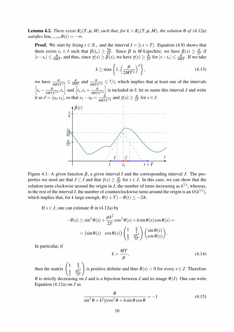
Figure 4.1: A given function β , a given interval I and the corresponding interval J. The pro-perties we need are that J ⊂ I and that γ(s) ≥ µ

2T for s ∈ J. In this case, we can show that thesolution turns clockwise around the origin in J, the number of turns increasing as k3/4, whereas,in the rest of the interval I, the number of counterclockwise turns around the origin is an O(k1/2),which implies that, for k large enough, θ(t +T )−θ(t)≤−2π .

If s ∈ J, one can estimate θ in (4.12a) by

−θ(s)≥ sin2θ(s)+

µk2

2Tcos2

θ(s)+hsinθ(s)cosθ(s) =

=(sinθ(s) cosθ(s)

)(1 h2

h2

µk2

2T

)(sinθ(s)cosθ(s)

).

In particular, if

k >MTµ

, (4.14)

then the matrix

(1 h

2h2

µk2

2T

)is positive definite and thus θ(s)< 0 for every s ∈ J. Therefore

θ is strictly decreasing on J and is a bijection between J and its image θ(J). One can writeEquation (4.12a) on J as

θ

sin2θ + k2γ cos2 θ +hsinθ cosθ

=−1 (4.15)

16

and, by integrating from s0 to s1 and using the relationw π/2

−π/2

dθ

sin2θ +acos2 θ +bsinθ cosθ

=2π√

4a−b2, a > 0, b2 < 4a,

which can be calculated directly by the change of variables t = tanθ , we obtain

µ

4MT k1/4= s1− s0 =−

w s1

s0

θ(s)sin2

θ(s)+ k2γ(s)cos2 θ(s)+hsinθ(s)cosθ(s)ds≤

≤w

θ(s0)

θ(s1)

dθ

sin2θ + k2µ

2T cos2 θ +hsinθ cosθ

≤

≤w

θ(s1)+π(N+1)

θ(s1)

dθ

sin2θ + k2µ

2T cos2 θ +hsinθ cosθ

=

=2π(N +1)√

2k2µ

T −h2=

2π(N +1)√2µ

T k2−2Mk,

(4.16)

where N is the number of rotations of angle π done during the interval J, i.e.,

N =

⌊θ(s0)−θ(s1)

π

⌋.

Therefore

θ(s0)−θ(s1)≥ πN ≥ k3/4 µ

8MT

√2µ

T− 2M

k−π. (4.17)

On the other hand, one can estimate θ in (4.12a) for every s ∈ I by

θ(s)≤ h,

so thatθ(s0)−θ(t)≤ h(s0− t), θ(t +T )−θ(s1)≤ h(t +T − s1). (4.18)

Thus, by (4.17) and (4.18), we obtain

θ(t +T )−θ(t)≤√

2kMT − k3/4 µ

8MT

√2µ

T− 2M

k+π.

The expression on the right-hand side tends to −∞ as k→+∞ and the parameters T , µ andM are fixed, and so there exists K?(T,µ,M) such that, if

k ≥ K?(T,µ,M), (4.19)

then√

2kMT − k3/4 µ

8MT

√2µ

T− 2M

k+π ≤−2π

and thusθ(t +T )−θ(t)≤−2π.

We group conditions (4.13), (4.14) and (4.19) in a single one by setting

K2(T,µ,M) = max

1,(

µ

2MT 2

)4,MTµ

,K?(T,µ,M)

17

and asking thatk > K2(T,µ,M).

Under this condition, the solution completes at least one complete clockwise rotation bythe end of the interval [t, t +T ]. This result is true for every t ∈ R+ and thus an immediateinduction shows that

θ(t +nT )−θ(t)≤−2nπ

for every n ∈ N, so that, for every t ∈ R+,

θ(t) = θ (t/TT + bt/TcT )≤ θ (t/TT )−2bt/Tcπ (4.20)

where x = x−bxc ∈ [0,1). Since θ is bounded on the interval [0,T ], Inequality (4.20)shows that limt→+∞ θ(t) =−∞, thus completing the proof.

4.3.3 Decomposition of the time in intervals I+ and I0

Using Lemma 4.2, we can decompose R+ in a sequence of intervals (depending on α) on whichthe solution rotates by an angle π around the origin. More precisely, we define the sequence(tn)n∈N by induction as

t0 = inft ≥ 0 | θ(t)π∈ Z,

tn = inft ≥ tn−1 |θ(t) = θ(tn−1)−π, n≥ 1,(4.21)

and the continuity of θ and Lemma 4.2 show that this sequence is well defined. We also definethe sequence of intervals (In)n∈N by In = [tn−1, tn] for n ≥ 1 and I0 = [0, t0]. The constructionmeans thus that we wait until the solution passes through the axis y1 for the first time and, fromthis moment, we divide the time in intervals on which the solution rotates by an angle π aroundthe origin, going back to the axis y1.

We can show a first result about the behavior of θ on these intervals.

Lemma 4.3. Let n≥ 1. Then, for every t ∈ In = [tn−1, tn], one has

θ(tn)≤ θ(t)≤ θ(tn−1). (4.22)

Proof. The first inequality in (4.22) is a consequence of the definition of tn: if there wast ∈ In with θ(t) < θ(tn), then, by the continuity of θ , there would be s ∈ ]tn−1, t[ such thatθ(s) = θ(tn) = θ(tn−1)− π , and thus, by definition of tn, we would have tn ≤ s < t < tn,which is a contradiction, and thus we have θ(t)≥ θ(tn) for every t ∈ In.

The second inequality in (4.22) can also be proved by contradiction. We suppose thatthere exists t ∈ In such that θ(t) > θ(tn−1). Then, by continuity of θ , there exists s0,s1 ∈[tn−1, t] such that θ(s0) = θ(tn−1), θ(s1) > θ(tn−1) and θ(s) ∈ [θ(tn−1),θ(tn−1) + π/2]for every s ∈ [s0,s1]. But we have that θ(tn−1) = 0 mod π , so that sinϑ cosϑ ≥ 0 forϑ ∈ [θ(tn−1),θ(tn−1) + π/2], and thus, by (4.12a), θ(s) ≤ 0 for almost every s ∈ [s0,s1],which contradicts the fact that θ(s0) = θ(tn−1) and θ(s1) > θ(tn−1) since θ is absolutelycontinuous. We then have θ(t)≤ θ(tn−1) for every t ∈ In.

We now split the intervals of the sequence (In)n∈N∗ into two classes, I+ and I0, according tothe behavior of β on these intervals. We define

I+ = In |n ∈ N∗,∃t ∈ In,β (t)≥ 2/√

k ,I0 = In |n ∈ N∗,∀t ∈ In,β (t)< 2/

√k .

18

t

θ(t)θ(tn−1)+ π/2

θ(tn−1)

θ(tn)

tn−1 tnts0 s1

Figure 4.2: Contradiction used to prove the second inequality in (4.22). The existence of t suchthat θ(t) > θ(tn−1) makes it possible to construct an interval [s0,s1] where θ(s1) > θ(s0) butθ ≤ 0, thus leading to a contradiction.

4.3.4 Estimations on intervals I+

We start by studying the intervals in the class I+. We first claim that, for k large enough, wehave γ(t)≥ 1/

√k for almost every t ∈ I and every I ∈ I+.

Lemma 4.4. There exists K3(M) such that, for k > K3(M) and for every I ∈ I+, one has β (t)≥1/√

k for every t ∈ I and γ(t)≥ 1/√

k for almost every t ∈ I.

Proof. We fix an interval I = [tn−1, tn] ∈ I+ and we note t? ∈ I an element of I such thatβ (t?) ≥ 2/

√k. Since β is M-Lipschitz, for every t such that |t− t?| ≤ 1

M√

k, we have 1/

√k ≤

β (t)≤ 3/√

k. In particular, since γ(t)≥ β (t) on R+, we have γ(t)≥ 1/√

k for |t− t?| ≤ 1M√

k.

The idea is to show that, for k large enough, one must have I ⊂[t?− 1

M√

k, t?+ 1

M√

k

],

which we do by saying that, for k large enough, the number of rotations of angle π aroundthe origin done on each of the intervals

[t?− 1

M√

k, t?]

and[t?, t?+ 1

M√

k

]is larger than 1,

which is the number of rotations of angle π around the origin done on I.We take s0,s1 ∈

[t?− 1

M√

k, t?+ 1

M√

k

], s0 < s1. For every s ∈ [s0,s1], we have

−θ(s)≥ sin2θ(s)+ k3/2 cos2

θ(s)+hsinθ(s)cosθ(s) =

=(sinθ(s) cosθ(s)

)(1 h2

h2 k3/2

)(sinθ(s)cosθ(s)

),

and the matrix(

1 h2

h2 k3/2

)is positive definite if

k >M2

4. (4.23)

We take k satisfying (4.23). We can thus write Equation (4.12a) on [s0,s1] as (4.15), and byintegrating as in (4.16), we obtain

s1− s0 ≤w

θ(s1)+π(N(s0,s1)+1)

θ(s1)

dθ

sin2θ + k3/2 cos2 θ +hsinθ cosθ

=

=2π(N(s0,s1)+1)√

4k3/2−2Mk=

π(N(s0,s1)+1)

k3/4√

1− M2k1/2

,

19

where

N(s0,s1) =

⌊θ(s0)−θ(s1)

π

⌋is the number of rotations of angle π around the origin done by the solution between s0 ands1. Hence

N(s0,s1)≥ k3/4 (s1− s0)

π

√1− M

2k1/2−1,

and, in particular,

N(

t?− 1M√

k, t?)≥ k1/4

Mπ

√1− M

2k1/2−1,

N(

t?, t?+ 1M√

k

)≥ k1/4

Mπ

√1− M

2k1/2−1.

For M fixed, we have k1/4

Mπ

√1− M

2k1/2 −1−−−−→k→+∞

+∞, and thus there exists K?(M) such that,

fork > K?(M), (4.24)

one hask1/4

Mπ

√1− M

2k1/2−1 > 1.

ThereforeN(

t?− 1M√

k, t?)> 1, N

(t?, t?+ 1

M√

k

)> 1,

and thenθ(t?)−θ

(t?+ 1

M√

k

)> π, θ

(t?− 1

M√

k

)−θ(t?)> π. (4.25)

By definition of I, we have θ(tn−1)−θ(tn) = π , and, by Lemma 4.3, θ(tn)≤ θ(t)≤ θ(tn−1)for every t ∈ I; the fact that t? ∈ I and (4.25) show that t?− 1

M√

k/∈ I, t?+ 1

M√

k/∈ I, from

where we conclude that

t?− 1M√

k< tn−1, t?+ 1

M√

k> tn,

and then I ⊂[t?− 1

M√

k, t?+ 1

M√

k

]. We now group (4.23) and (4.24) by setting

K3(M) = max

M2

4,K?(M)

and asking that

k > K3(M).

Under this hypothesis, we have I ⊂[t?− 1

M√

k, t?+ 1

M√

k

]and, since β (t) ≥ 1/

√k for every

t such that |t− t?| ≤ 1M√

kand γ(t) ≥ 1/

√k for almost every t such that |t− t?| ≤ 1

M√

k, we

obtain the desired result.

By using this result, we can estimate the divergence rate of the solution over an interval onthe class I+.

20

Lemma 4.5. There exists K4(M) such that, for k > K4(M) and for every I = [tn−1, tn] ∈ I+, thesolution of (4.12c) satisfies

r(tn)≤ r(tn−1)e4Mk1/2(tn−tn−1). (4.26)

Proof. We start by takingk > K3(M), (4.27)

so that we can apply Lemma 4.4 and obtain that β (t)≥ 1/√

k for every t ∈ I and γ(t)≥ 1/√

k

for almost every t ∈ I. We thus have, for t ∈ I,

−θ(t)≥ sin2θ(t)+ k3/2 cos2

θ(t)+hsinθ(t)cosθ(t) =

=(sinθ(t) cosθ(t)

)(1 h2

h2 k3/2

)(sinθ(t)cosθ(t)

)> 0

for, since k > K3(M), we have in particular (4.23) and thus the above matrix is positivedefinite. Hence θ is a continuous strictly decreasing function on I, being thus a bijectionbetween I = [tn−1, tn] and its image [θ(tn),θ(tn−1)]. We note by τ the inverse of θ , definedon [θ(tn),θ(tn−1)]; τ thus satisfies

dτ

dϑ(ϑ) =

1θ(τ(ϑ))

=− 1sin2

ϑ + k2γ(τ(ϑ))cos2 ϑ +hsinϑ cosϑ. (4.28)

We note ρ = r τ , and hence, by using Equations (4.12c) and (4.28), we have

ddϑ

lnρ =− sinϑ cosϑ(1− k2γ τ(ϑ))−hsin2ϑ

sin2ϑ + k2γ τ(ϑ)cos2 ϑ +hsinϑ cosϑ

.

We can integrate this expression from θ(tn) to θ(tn−1) = θ(tn)+π , obtaining

lnr(tn)

r(tn−1)=

wθ(tn)+π

θ(tn)F(ϑ ,γ τ(ϑ))dϑ

with

F(ϑ ,γ) =sinϑ cosϑ(1− k2γ)−hsin2

ϑ

sin2ϑ + k2γ cos2 ϑ +hsinϑ cosϑ

.

If γ0 ≥ 1/√

k is constant, then

wθ(tn)+π

θ(tn)F(ϑ ,γ0)dϑ ≤ 0; (4.29)

to see so, it suffices to see that, since F is π-periodic on ϑ , this integral can be taken in anyinterval of length π , and that, by making the change of variables given by t = tanϑ , one has

w π/2

−π/2F(ϑ ,γ0)dϑ =

w +∞

−∞

(1− k2γ0)t−ht2

(t2 +ht + k2γ0)(t2 +1)dt ≤

≤w +∞

−∞

(1− k2γ0)t(a0t2 +b0)(t2 +1)

dt = 0

with a0 = k2γ0−h2/4k2γ0+h2/4 , b0 = k2γ0

2 −h2

8 ; these are both positive since γ0 ≥ 1/√

k and k satisfies

(4.23), and they are chosen in such a way that t2 +ht + k2γ0 ≥ a0t2 +b0 for every t ∈ R.

21

By (4.29), we have

lnr(tn)

r(tn−1)≤

wθ(tn)+π

θ(tn)[F(ϑ ,γ τ(ϑ))−F(ϑ ,γ0)]dϑ . (4.30)

We compute∂F∂γ

(ϑ ,γ) =− k2 sinϑ cosϑ

(sin2ϑ + k2γ cos2 ϑ +hsinϑ cosϑ)2

,

and thus, for t ∈ I,∣∣∣∣∂F∂γ

(ϑ ,γ(t))∣∣∣∣≤ k2 |sinϑ | |cosϑ |

(sin2ϑ + k3/2 cos2 ϑ +hsinϑ cosϑ)2

.

We now take γ0 = β (tn−1) in (4.30), obtaining

lnr(tn)

r(tn−1)≤

wθ(tn)+π

θ(tn)

k2 |sinϑ | |cosϑ |(sin2

ϑ + k3/2 cos2 ϑ +hsinϑ cosϑ)2|γ τ(ϑ)−β (tn−1)|dϑ .

(4.31)For almost every t ∈ I, one can estimate

|γ(t)−β (tn−1)| ≤ |β (t)−β (tn−1)|+∣∣∣∣ α(t)

2k

∣∣∣∣≤M(tn− tn−1)+M2k

. (4.32)

We take k satisfying (4.11), which means that 0 ≤ γ(t) ≤ 1 for almost every t ∈ R+, andthus, by integrating (4.15) from tn−1 to tn, we obtain

tn− tn−1 =−w tn

tn−1

θ(s)sin2

θ(s)+ k2γ(s)cos2 θ(s)+hsinθ(s)cosθ(s)ds≥

≥w

θ(tn)+π

θ(tn)

dθ

sin2θ + k2 cos2 θ +hsinθ cosθ

=π

k√

1− M2k

,

from where we get1k≤ tn− tn−1

π

and thus (4.32) becomes

|γ(t)−β (tn−1)| ≤M(1+ 1

2π

)(tn− tn−1)< 2M(tn− tn−1).

We use this estimate in (4.31), which leads to

lnr(tn)

r(tn−1)≤ 2k2M(tn− tn−1)

wθ(tn)+π

θ(tn)

|sinϑ | |cosϑ |(sin2

ϑ + k3/2 cos2 ϑ +hsinϑ cosϑ)2dϑ . (4.33)

In order to calculate the integral in (4.33), we use the π-periodicity of the integrand and that,for a > 0 and b2 < 4a, we have

w π/2

−π/2

|sinϑ | |cosϑ |(sin2

ϑ +acos2 ϑ +bsinϑ cosϑ)2dϑ =

1A+

BA3/2

arctan(B/√

A)≤ 1A

(1+

π

2C)

22

with A = a− b2/4 > 0, B = b/2 and C = B/√

A = b√4a−b2 . Applying this to (4.33) gives

lnr(tn)

r(tn−1)≤ 2k1/2M(tn− tn−1)

1− M2k1/2

(1+

π

2

√kM

2k3/2− kM

)

and, since 11− M

2k1/2

(1+ π

2

√kM

2k3/2−kM

)−−−−→k→+∞

1, there exists K?(M) such that, if

k ≥ K?(M), (4.34)

then 11− M

2k1/2

(1+ π

2

√kM

2k3/2−kM

)≤ 2, and thus

lnr(tn)

r(tn−1)≤ 4k1/2M(tn− tn−1).

We group hypothesis (4.11), (4.27) and (4.34) done on k by setting

K4(M) = maxK1(M),K3(M),K?(M)

and requiring thatk > K4(M).

Under this hypothesis, we obtain

r(tn)≤ r(tn−1)e4Mk1/2(tn−tn−1).

4.3.5 Estimations on intervals I0

Lemma 4.5 allows us to estimate the growth of the norm after a rotation of angle π in an intervalof the class I+. We now wish to obtain a similar result for the intervals of the class I0; to do so,we start by obtaining a first result characterizing the duration of these intervals and the behaviorof γ .

Lemma 4.6. There exists K5(T,µ,M) such that, if k>K5(T,µ,M), then for every I = [tn−1, tn]∈I0 one has γ(t)≤ 3/

√k for almost every t ∈ I and

π

1+h+3k3/2≤ tn− tn−1 < T.

Proof. We fix I = [tn−1, tn] ∈ I0. Ifk ≥M2, (4.35)

then 0≤ γ(t)−β (t)≤ Mk ≤

1√k, and thus γ(t)≤ 3/

√k almost everywhere on I. Also, if

k >(

8T3µ

)2

, (4.36)

23

we have β (t) < 2/√

k < 3µ

4T , and thus, by the persistence of excitation (4.9) of β , we obtainthat tn−tn−1 < T . Furthermore, by (4.12a), we obtain−θ ≤ 1+3k3/2+h almost everywhereon I, and then by integrating on I we deduce that tn− tn−1 ≥ π

1+h+3k3/2 . So, by defining

K5(T,µ,M) = max

M2,

(8T3µ

)2,

inequalities (4.35) and (4.36) are satisfied if

k > K5(T,µ,M),

thus giving the desired result.

We suppose from now on that k > K5(T,µ,M). Our goal now is to obtain a result similarto Lemma 4.5 for the case of an interval I ∈ I0. Le us start by defining the class D(T,µ,M,k)where we take γ .

Definition 4.7. We define the class D(T,µ,M,k) as

D(T,µ,M,k) =

α(1− 1

4α)+

M− α

2k, α ∈D(T,µ,M)

.

We fix I = [tn−1, tn] ∈ I0. We remark that, if γ ∈D(T,µ,M,k), then, for every t0 ∈ R+, thefunction t 7→ γ(t + t0) is also in D(T,µ,M,k). Up to a translation in time, we can then supposeI = [0,τ] with τ = tn− tn−1 ∈

[π

1+h+3k3/2 ,T)

. The solution r(τ) of (4.12c) at time τ can bewritten as

r(τ) = r(0)eΛτ

for a certain constant Λ. We know by construction that r(0) is in the axis y1 and thus, sinceSystem (4.8) is linear, we conclude by homogeneity that Λ does not depend on the particularvalue of r(0), depending only on τ and r(τ). Our goal is to estimate Λ uniformly with respectto the class of signals γ ∈D(T,µ,M,k) and with respect to all intervals I ∈ I0 for a given choiceof γ . We can thus estimate Λ by the maximal value of 1

τln ‖y(τ)‖‖y(0)‖ over all τ ∈

[π

1+h+3k3/2 ,T)

andall γ ∈D(T,µ,M,k) with γ(t)< 3/

√k, where y is a solution of (4.8) with both y(0) and y(τ) in

the axis y1. That is, Λ is estimated by the solution of the problem

Find sup1τ

ln‖y(τ)‖‖y(0)‖

with

τ ∈[

π

1+h+3k3/2,T], γ ∈D(T,µ,M,k), γ(t)< 3/

√k on [0,τ],

y =(

0 1−k2γ(t) −h

)y, y(0) =

(y1(0)

0

), y(τ) =

(ξ

0

),

y1(0),ξ ∈ R∗, y1(0)ξ < 0.

(4.37)

We can choose y1(0) =−1 without loss of generality since the equation satisfied by y is linear.We can also see that, by enlarging the class where we take γ and taking γ ∈ L∞([0,τ], [0,3/√γ]),

24

we obtain a problem whose solution is bigger than the solution of (4.37), and thus Λ is alsoestimated by the solution of the problem

Find sup1τ

ln‖y(τ)‖ with

τ ∈[

π

1+h+3k3/2,T], I = [0,τ], γ ∈ L∞(I, [0,1]),

y =(

0 1−3k3/2γ(t) −h

)y, y(0) =

(−10

), y(τ) ∈

(ξ

0

), ξ ∈ R+

.

(4.38)

We now precise and summarize all the preceding discussion in the following result.

Lemma 4.8. Let ΛΛΛ(T,M,k) be the solution of Problem (4.38) and take K5(T,µ,M) as in Lemma4.6. If k > K5(T,µ,M), then, for every γ ∈ D(T,µ,M,k) and for every I = [tn−1, tn] ∈ I0, wehave

r(tn)≤ r(tn−1)eΛΛΛ(T,M,k)(tn−tn−1). (4.39)

Proof. Fix γ ∈D(T,µ,M,k) and I = [tn−1, tn] ∈ I0. We take k > K5(T,µ,M) in order to ap-ply Lemma 4.6. We define τ = tn− tn−1, and thus Lemma 4.6 shows that τ ∈

[π

1+h+3k3/2 ,T)

and γ(t)≤ 3/√

k for almost every t ∈ I.We note γ(t) =

√k

3 γ(t + tn−1) for every t ∈ I, and thus γ ∈ L∞(I, [0,1]) with I = [0,τ].We note by y the solution of (4.8) with a non-zero initial condition and by z the functiondefined by z(t) =− sign(y1(tn−1))

‖y(tn−1)‖ y(t+ tn−1). We see that z is well defined since ‖y(tn−1)‖ 6= 0,and z satisfies

z =(

0 1−k2γ(t + tn−1) −h

)z =

(0 1

−3k3/2γ(t) −h

)z.

By definition of I, both y(tn−1) and y(tn) are on the axis y1, on opposite sides of the origin,and thus both z(0) and z(τ) are on the axis z1 on opposite sides of the origin; by the definitionof z, we can thus write

z(0) =(−10

), z(τ) ∈

(ξ

0

), ξ ∈ R∗+

.

It suffices now to see that, by the definition of ΛΛΛ(T,M,k), one has

1τ

ln‖z(τ)‖ ≤ΛΛΛ(T,M,k),

and thus‖z(τ)‖ ≤ eΛΛΛ(T,M,k)τ .

By the definition of z and τ , we obtain (4.39).

We can now concentrate on the problem of solving (4.38). We start by proving that the supin this problem is attained.

Lemma 4.9. Let k > K5(T,µ,M) where K5 is defined in Lemma 4.6 and we note ΛΛΛ(T,M,k) thesolution of Problem (4.38). Then there exist τ? ∈

[π

1+h+3k3/2 ,T]

and γ? ∈ L∞(I?, [0,1]), whereI? = [0,τ?], such that, if y? denotes the solution of

y? =(

0 1−3k3/2γ?(t) −h

)y?, y?(0) =

(−10

),

25

then

y?(τ) ∈(

ξ

0

), ξ ∈ R+

and

1τ?

ln‖y?(τ?)‖=ΛΛΛ(T,M,k).

Proof. We start by taking a sequence (τn,γn)n∈N with τn ∈[

π

1+h+3k3/2 ,T], In = [0,τn] and

γn ∈ L∞(In, [0,1]), such that, by denoting yn the solution ofyn =

(0 1

−3k3/2γn(t) −h

)yn,

yn(0) =(−10

),

(4.40)

we havelim

n→+∞

1τn

ln‖yn(τn)‖=ΛΛΛ(T,M,k);

such a maximizing sequence exists by the definition of sup. Up to defining γn as 0 outside In,we can suppose that γn ∈ L∞(I, [0,1]) where I = [0,T ] and thus, by weak-? compactness ofthis space and by the compactness of

[π

1+h+3k3/2 ,T], we can find a subsequence of (γn)n∈N

converging weak-? to a certain function γ? ∈ L∞(I, [0,1]) and such that the correspondingsubsequence of (τn)n∈N converges to τ? ∈

[π

1+h+3k3/2 ,T]; to simplify the notation, we still

write (γn)n∈N and (τn)n∈N for these subsequences.We remark that γ? is equal 0 almost everywhere outside I? = [0,τ?] since, for every

function ϕ ∈ L1([τ?,T ]), one hasw T

τ?

γ?(t)ϕ(t)dt = limn→+∞

w T

τ?

γn(t)ϕ(t)dt

and ∣∣∣∣w T

τ?

γn(t)ϕ(t)dt∣∣∣∣=0 if τn ≤ τ?,∣∣∣w τn

τ?

γn(t)ϕ(t)dt∣∣∣≤ w

τn

τ?

|ϕ(t)|dt −−−−→n→+∞

0 if τn > τ?.

We consider γ? ∈ L∞(I?, [0,1]). We note by y? the solution corresponding to γ?, i.e., thesolution of

y? =(

0 1−3k3/2γ?(t) −h

)y?,

y?(0) =(−10

).

(4.41)

By defining γn and γ? to be 0 on [0,T ] outside their respective definition intervals In andI?, we can consider the solutions yn and y? of (4.40) and (4.41) to be defined on [0,T ] and,in this case, up to extracting a subsequence, we have limn→+∞ yn = y? uniformly on [0,T ].In fact, let us note en = yn− y?. We write

An(t) =(

0 1−3k3/2γn(t) −h

), B =

(0 0

−3k3/2 0

).

26

The function en satisfiesen(t) = An(t)en(t)+(γn(t)− γ?(t))By?(t),

en(0) = (0,0)T,

and, by integrating this equation, we get

en(t) =w t

0An(s)en(s)ds+hn(t), hn(t) =

w t

0(γn(s)− γ?(s))By?(s)ds. (4.42)

We now apply Gronwall’s Lemma to ‖en(t)‖, obtaining

‖en(t)‖ ≤ ‖hn(t)‖+w t

0‖hn(s)‖‖An(s)‖e

r ts ‖An(s′)‖ds′ds. (4.43)

If t is fixed, the weak-? convergence of γn to γ? shows that limn→+∞ hn(t) = 0 for everyt ∈ [0,T ] and, furthermore, the sequence (hn)n∈N is uniformly bounded on [0,T ], whichshows that, by the Dominated Convergence Theorem,

limn→+∞

w t

0‖hn(s)‖‖An(s)‖e

r ts ‖An(s′)‖ds′ds = 0

for every t ∈ [0,T ], since (‖An‖)n∈N is also uniformly bounded. Thus limn→+∞ en(t) = 0 forevery t ∈ [0,T ]. Since (hn)n∈N is uniformly bounded, (en)n∈N is also because of (4.43), and(4.42) shows that, for t > t ′,

en(t)− en(t ′) =w t

t ′An(s)en(s)ds+

w t

t ′(γn(s)− γ?(s))By?(s)ds,

which, with the uniform bound of (en)n∈N, shows that this sequence is equicontinuous.Hence, by Arzelà-Ascoli Theorem, up to taking a subsequence, (en)n∈N converges uni-formly and, since it converges punctually to 0, its uniform limit is the function 0, whichshows that limn→+∞ yn = y? uniformly on [0,T ].

The uniform convergence enables us to show the conclusion of the lemma. In fact, sinceyn(τn) ∈

(ξ 0

)T, ξ ∈ R+

and limn→+∞ yn(τn) = y?(τ?) by uniform convergence, we

conclude that y?(τ?) ∈(

ξ 0)T

, ξ ∈ R+

since this set is closed. The uniform conver-

gence of yn to y? also shows that

1τ?

ln‖y?(τ?)‖= limn→+∞

1τn

ln‖yn(τn)‖=ΛΛΛ(T,M,k),

which completes the proof.

Now that we know that the sup in Problem (4.38) is attained, we can use Pontryagin Maxi-mum Principle to characterize the trajectory y? that attains the sup of (4.38). We use as referencethe statement of Pontryagin Maximum Principle given in Theorem 7.3 of [2], which we recallhere.

Theorem 4.10 (Pontryagin Maximum Principle). Consider the problem

maxγ∈U

φ0(τ,y(τ)) (4.44a)

27

for the system described by the equations

y = f (y(t),γ(t)), y(0) = y0, γ(t) ∈U almost everywhere, (4.44b)

where the terminal time τ and the terminal point y(τ) are subject to the constraints

φi(τ,y(τ)) = 0, i = 1, . . . ,n. (4.44c)

We also suppose that f is continuous on Ω×U, where Ω ⊂ Rd is open, that f is continu-ously differentiable with respect to y and that the functions φi, i = 0, . . . ,n are continuouslydifferentiable. Let τ? and γ? : [0,τ?]→U maximize (4.44a), with γ? bounded, and let y? be thecorresponding trajectory, solution of (4.44b). We suppose that the vectors

(∂φi∂ t ,

∂φi∂y1

, . . . , ∂φi∂yd

),

i = 1, . . . ,n, are linearly independent at the point (τ?,y?(τ?)). The there exists a nontrivialabsolutely continuous row vector p such that

p(t) =−p(t) ·Dy f (y?(t),γ?(t)), (4.45a)p(t) · f (y?(t),γ?(t)) = max

ω∈Up(t) · f (y?(t),ω) (4.45b)

at almost every time t ∈ [0,τ?]. Moreover, there exist constants λ0, . . . ,λn with λ0 ≥ 0 such that

p(τ?) =n

∑i=0

λi∇φi(τ?,y?(τ?)) 6= 0, (4.45c)

maxω∈Up(τ?) · f (y?(τ?),ω)=−

n

∑i=0

λi∂φi

∂ t(τ?,y?(τ?)) (4.45d)

where ∇φi =(

∂φi∂y1

, . . . , ∂φi∂yd

). Finally, the function t 7→ p(t) · f (y?(t),γ?(t)) is constant almost

everywhere.

We can then apply Theorem 4.10 to Problem (4.38). The function φ0 in the statement of thetheorem and the function f defining the system are

φ0(t,y) =1t

ln‖y‖ , f (y,γ) =(

0 1−3k3/2γ −h

)y. (4.46a)

Still in the notations of Theorem 4.10, we have

U = [0,1], U= L∞([0,τ], [0,1]). (4.46b)

The constraint on the final point can be written as φ1(τ,y(τ)) = 0 with

φ1(t,y) = y2, (4.46c)

and then n = 1. We also remark that f , φ0 and φ1 satisfy the regularity hypothesis stated inthe theorem. Then, given τ? and γ? as in the statement of Lemma 4.9 and the correspondingsolution y?, the conclusions of Theorem 4.10 are valid: there exist a vector p and constantsλ0,λ1 satisfying (4.45). We now want to gather, from these conclusions, properties that willallow us to characterize γ? and y?.

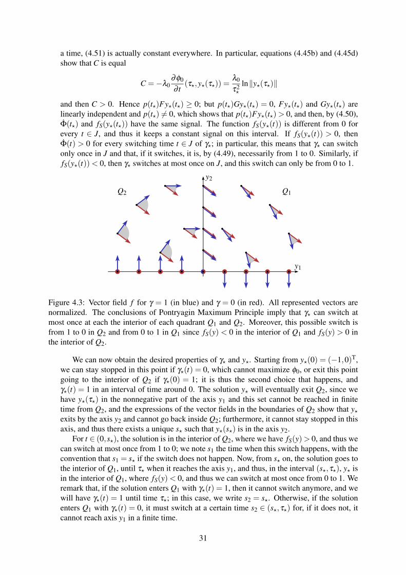
Lemma 4.11. Let τ?, γ? and y? be as in the statement of Lemma 4.9. Then γ? takes its values on0,1. Moreover, there exist s1,s2 ∈ (0,τ?) with s1 ≤ s2 such that γ?(t) = 1 if t ∈ [0,s1)∪(s2,τ?]and γ?(t) = 0 if t ∈ (s1,s2). The solution y? is included in the quadrant Q2 = (y1,y2) | y1 ≤0, y2 ≥ 0 during the interval [0,s1] and in the quadrant Q1 = (y1,y2) |y1 ≥ 0, y2 ≥ 0 during[s2,τ?].

28

Proof. First of all, let us explicitly write the conclusions of Theorem 4.10 in the case of(4.46). We note by p the row vector whose existence is given by Theorem 4.10; the equation(4.45a) it satisfies is

p =−p(

0 1−3k3/2γ?(t) −h

),

that is, p1(t) = 3k3/2

γ?(t)p2(t),p2(t) = hp2(t)− p1(t).

(4.47)

We havep · f (y?,ω) = p1y2?−3k3/2

ω p2y1?−hp2y2?,

and so the maximization condition (4.45b) is

γ?(t)p2(t)y1?(t) = minω∈[0,1]

ω p2(t)y1?(t). (4.48)

We can now show that γ? takes its values on 0,1. We define the switching function Φ

byΦ(t) = p2(t)y1?(t)

and then, by (4.48), γ? can be written in function of Φ as

γ?(t) =

0 si Φ(t)> 0,1 si Φ(t)< 0.

(4.49)

We remark that, if Φ(t) 6= 0 almost everywhere on [0,τ?], the function γ? is defined almosteverywhere by (4.49), and, in particular, it takes its values in 0,1. We also remark that Φ

is absolutely continuous and

Φ(t) = hp2(t)y1?(t)− p1(t)y1?(t)+ p2(t)y2?(t);

Φ is then also absolutely continuous, which shows that Φ is of class C1.We now want to show that Φ cannot be zero on an interval. Indeed, we suppose, by

contradiction, that Φ is zero on a certain interval, and we fix an open subinterval J where Φ

is zero. For every s ∈ J, we have Φ(s) = 0 and Φ(s) = 0. We can then write

Φ(t) =(

p1(t) p2(t))( 0

y1?(t)

), Φ(t) =

(p1(t) p2(t)

)( −y1?(t)y2?(t)+hy1?(t)

).

By Theorem 4.10, p is nontrivial, and the system (4.47) it satisfies is linear, which meansthat the vector p is never equal to zero. Conditions Φ(s) = 0 and Φ(s) = 0 mean that both(0,y1?(s))T and (−y1?(s),y2?(s)+hy1?(s))T are orthogonal to p(s)T; they are then parallel,which means that y1?(s) = 0 for every s∈ J. But y1? = y2?, which then shows that y2?(s) = 0for s ∈ J, and then, by uniqueness of the solution, (y1?,y2?)

T is the solution equal to 0 overall R+, which is a contradiction. We thus conclude that Φ cannot be zero on an interval, andthus (4.49) defines γ? almost everywhere. In particular, γ? takes its values on 0,1.

We now want to show the other results on the statement of the lemma. The method weuse here is inspired on the one used on Section 7.3 of [1], where a result of the kind was

29

proved in the case of a time minimization problem of a control system linear in the control.We start by defining the matrices

F =

(0 10 −h

), G =

(0 01 0

),

in such a way that the function f of the control system y(t) = f (y(t),γ(t)) can be written as

f (y,γ) = Fy−3k3/2γGy.

We remark also that the switching function Φ and its derivative Φ can be written as

Φ(t) = p(t)Gy?(t), Φ(t) = p(t)[G,F ]y?(t)

where [G,F ] =GF−FG is the commutator of the matrices G and F . We define the functions

∆A(y) = det(Fy,Gy) =∣∣∣∣ y2 0−hy2 y1

∣∣∣∣= y1y2,

∆B(y) = det(Gy, [G,F ]y) =∣∣∣∣ 0 −y1y1 hy1 + y2

∣∣∣∣= y21.

The set ∆−1A (0), corresponding to the axis y1 and y2, is the set of points where the vector

fields defined by F and G are parallel and the set ∆−1B (0), corresponding to the axis y2, is

the set of points where the vector fields defined by G and [G,F ] are parallel. In particu-lar, outside ∆

−1A (0), Fy and Gy are two linearly independent vectors and they thus consti-

tute a basis of R2; hence there exist scalars fS(y) and gS(y) such that [G,F ]y = fS(y)Fy+gS(y)Gy for every y∈R2 \∆

−1A (0). We have ∆B(y) = det(Gy, [G,F ]y) = fS(y)det(Gy,Fy) =

− fS(y)∆A(y), which shows that

fS(y) =−∆B(y)∆A(y)

=−y1

y2.

We now want to characterize the switches of γ? when the trajectory is outside ∆−1A (0)∪

∆−1B (0), i.e., when the trajectory is not in one of the axis. We take an open time interval J

during which y? is outside the axes. In particular, fS(y?(t)) and gS(y?(t)) are defined forevery t ∈ J. If γ? switches at t? ∈ J, Equation (4.49) and the continuity of Φ show thatΦ(t?) = 0. We then have p(t?)Gy?(t?) = Φ(t?) = 0 and thus

Φ(t?) = p(t?)[G,F ]y?(t?) = fS(y?(t?))p(t?)Fy?(t?). (4.50)

Theorem 4.10 shows that t 7→ p(t) · f (y?(t),γ?(t)) is constant almost everywhere, i.e.,

t 7→ p(t)Fy?(t)−3k3/2γ?(t)p(t)Gy?(t) (4.51)

is constant almost everywhere; let us note C this constant. The functions t 7→ p(t)Fy?(t)and t 7→ p(t)Gy?(t) are absolutely continuous, which means that the only times when (4.51)may not be equal C is when γ? is discontinuous, i.e., the switching times. In particular,by taking the limit as t tends to a switching time by points were γ? is zero, we obtain thatp(t)Fy?(t) = C at the switching time, and, since we have p(t)Gy?(t) = Φ(t) = 0 in such

30

a time, (4.51) is actually constant everywhere. In particular, equations (4.45b) and (4.45d)show that C is equal

C =−λ0∂φ0

∂ t(τ?,y?(τ?)) =

λ0

τ2?

ln‖y?(τ?)‖

and then C > 0. Hence p(t?)Fy?(t?) ≥ 0; but p(t?)Gy?(t?) = 0, Fy?(t?) and Gy?(t?) arelinearly independent and p(t?) 6= 0, which shows that p(t?)Fy?(t?)> 0, and then, by (4.50),Φ(t?) and fS(y?(t?)) have the same signal. The function fS(y?(t)) is different from 0 forevery t ∈ J, and thus it keeps a constant signal on this interval. If fS(y?(t)) > 0, thenΦ(t) > 0 for every switching time t ∈ J of γ?; in particular, this means that γ? can switchonly once in J and that, if it switches, it is, by (4.49), necessarily from 1 to 0. Similarly, iffS(y?(t))< 0, then γ? switches at most once on J, and this switch can only be from 0 to 1.

y1

y2

Q2 Q1

Figure 4.3: Vector field f for γ = 1 (in blue) and γ = 0 (in red). All represented vectors arenormalized. The conclusions of Pontryagin Maximum Principle imply that γ? can switch atmost once at each the interior of each quadrant Q1 and Q2. Moreover, this possible switch isfrom 1 to 0 in Q2 and from 0 to 1 in Q1 since fS(y) < 0 in the interior of Q1 and fS(y) > 0 inthe interior of Q2.

We can now obtain the desired properties of γ? and y?. Starting from y?(0) = (−1,0)T,we can stay stopped in this point if γ?(t) = 0, which cannot maximize φ0, or exit this pointgoing to the interior of Q2 if γ?(0) = 1; it is thus the second choice that happens, andγ?(t) = 1 in an interval of time around 0. The solution y? will eventually exit Q2, since wehave y?(τ?) in the nonnegative part of the axis y1 and this set cannot be reached in finitetime from Q2, and the expressions of the vector fields in the boundaries of Q2 show that y?exits by the axis y2 and cannot go back inside Q2; furthermore, it cannot stay stopped in thisaxis, and thus there exists a unique s? such that y?(s?) is in the axis y2.

For t ∈ (0,s?), the solution is in the interior of Q2, where we have fS(y)> 0, and thus wecan switch at most once from 1 to 0; we note s1 the time when this switch happens, with theconvention that s1 = s? if the switch does not happen. Now, from s? on, the solution goes tothe interior of Q1, until τ? when it reaches the axis y1, and thus, in the interval (s?,τ?), y? isin the interior of Q1, where fS(y)< 0, and thus we can switch at most once from 0 to 1. Weremark that, if the solution enters Q1 with γ?(t) = 1, then it cannot switch anymore, and wewill have γ?(t) = 1 until time τ?; in this case, we write s2 = s?. Otherwise, if the solutionenters Q1 with γ?(t) = 0, it must switch at a certain time s2 ∈ (s?,τ?) for, if it does not, itcannot reach axis y1 in a finite time.

31

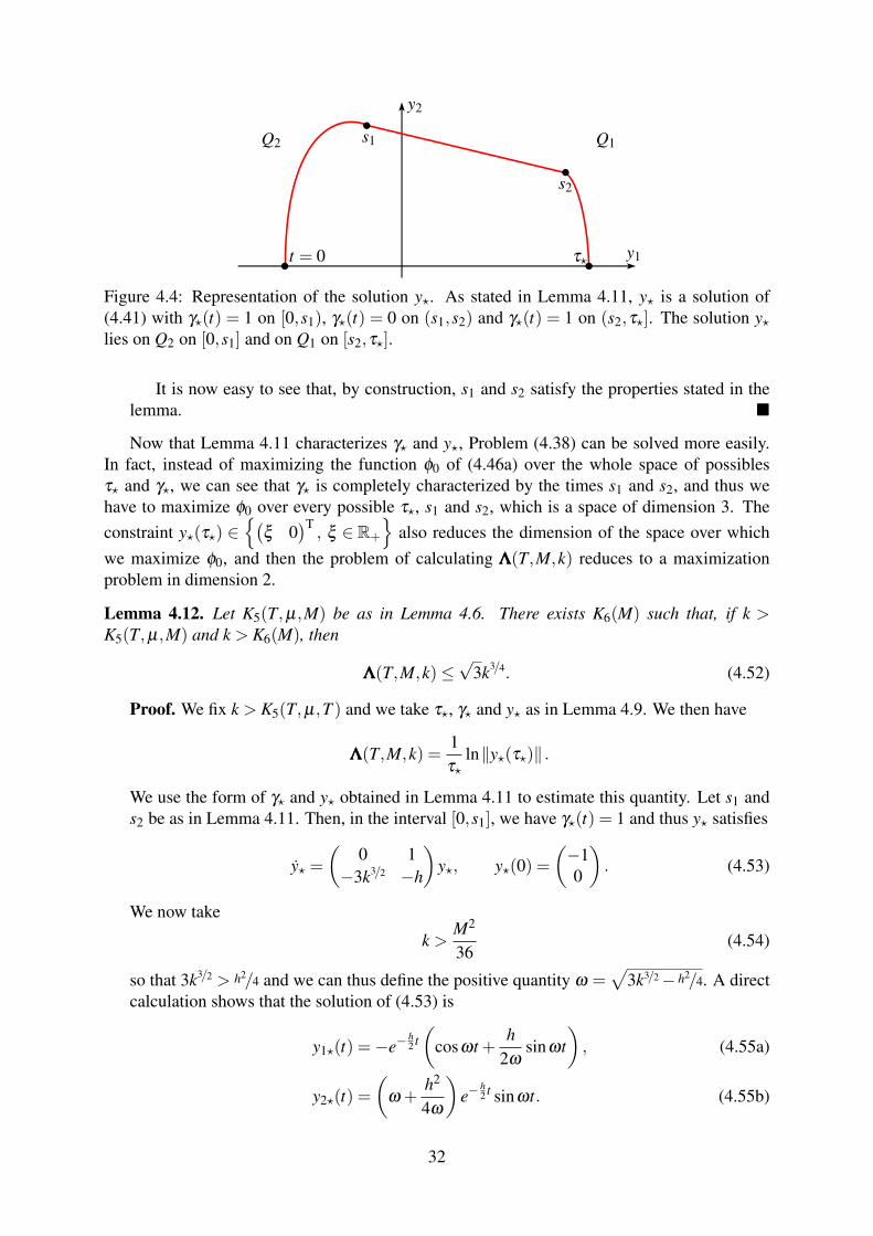
y1

y2

Q2 Q1

t = 0

s1

s2

τ?

Figure 4.4: Representation of the solution y?. As stated in Lemma 4.11, y? is a solution of(4.41) with γ?(t) = 1 on [0,s1), γ?(t) = 0 on (s1,s2) and γ?(t) = 1 on (s2,τ?]. The solution y?lies on Q2 on [0,s1] and on Q1 on [s2,τ?].

It is now easy to see that, by construction, s1 and s2 satisfy the properties stated in thelemma.

Now that Lemma 4.11 characterizes γ? and y?, Problem (4.38) can be solved more easily.In fact, instead of maximizing the function φ0 of (4.46a) over the whole space of possiblesτ? and γ?, we can see that γ? is completely characterized by the times s1 and s2, and thus wehave to maximize φ0 over every possible τ?, s1 and s2, which is a space of dimension 3. Theconstraint y?(τ?) ∈

(ξ 0

)T, ξ ∈ R+

also reduces the dimension of the space over which

we maximize φ0, and then the problem of calculating ΛΛΛ(T,M,k) reduces to a maximizationproblem in dimension 2.

Lemma 4.12. Let K5(T,µ,M) be as in Lemma 4.6. There exists K6(M) such that, if k >K5(T,µ,M) and k > K6(M), then

ΛΛΛ(T,M,k)≤√

3k3/4. (4.52)

Proof. We fix k > K5(T,µ,T ) and we take τ?, γ? and y? as in Lemma 4.9. We then have

ΛΛΛ(T,M,k) =1τ?

ln‖y?(τ?)‖ .

We use the form of γ? and y? obtained in Lemma 4.11 to estimate this quantity. Let s1 ands2 be as in Lemma 4.11. Then, in the interval [0,s1], we have γ?(t) = 1 and thus y? satisfies

y? =(

0 1−3k3/2 −h

)y?, y?(0) =

(−10

). (4.53)

We now take

k >M2

36(4.54)

so that 3k3/2 > h2/4 and we can thus define the positive quantity ω =√

3k3/2− h2/4. A directcalculation shows that the solution of (4.53) is

y1?(t) =−e−h2 t(

cosωt +h

2ωsinωt

), (4.55a)

y2?(t) =(

ω +h2

4ω

)e−

h2 t sinωt. (4.55b)

32

In the interval [s1,s2], we have γ?(t) = 0 and then the equation satisfied by y? is

y? =(

0 10 −h

)y?,

which yields the solution

y1?(t) =1h

(1− e−h(t−s1)

)y2?(s2)+ y1?(s1), (4.56a)

y2?(t) = e−h(t−s1)y2?(s1). (4.56b)

Finally, in the interval [s2,τ?], we have γ?(t) = 1 and thus the differential equation satis-fied by y? is the same as in (4.53), but we now consider the condition

y?(τ?) =(

ξ

0

)with ξ > 0. This yields the solution

y1?(t) = ξ e−h2 (t−τ?)

(cosω(t− τ?)+

h2ω

sinω(t− τ?)

), (4.57a)

y2?(t) =−ξ

(ω +

h2

4ω

)e−

h2 t sinω(t− τ?). (4.57b)

We haveΛΛΛ(T,M,k) =

1τ?

lnξ . (4.58)

To simplify the notation, we write σ = s2− s1. We want to estimate (4.58) in function ofs1 and σ and, to do so, we use the equalities obtained by saying that the solutions given in(4.56) and (4.57) coincide at the point s2. A development of these equalities yields

ξ eh2 (τ?−s2) sinω(τ?− s2) =

e−hσ

ω + h2

4ω

y2?(s1), (4.59a)

ξ eh2 (τ?−s2) cosω(τ?− s2) = y1?(s1)+ y2?(s1)

[1h

(1− e−hσ

)+

he−hσ

2ω2 + h2/4

], (4.59b)

and we can thus write ξ in function of s1, σ and τ?, and substitution in (4.58) shows that

ΛΛΛ(T,M,k) =−h(τ?−s2)+ln

(y1?(s1)+y2?(s1)

[1h(1−e−hσ)+ he−hσ

2ω2+h2/4

])2+

(e−hσ y2?(s1)

ω+ h24ω

)2

2[s1+σ+(τ?−s2)]. (4.60)

To simplify this expression, we first use that −h(τ?− s2)≤ 0 and τ− s2 ≥ 0. By the expres-sion (4.55b) of y2? in [0,s1], we estimate

e−hσ y2?(s1)

ω + h2

4ω

≤ sinωs1;

we recall that y2?(t) ≥ 0, which shows in particular by (4.55b) that sinωs1 ≥ 0, justifyingthus the previous estimate. We also have that y1?(s2)≥ 0 and y2?(s2)≥ 0, and then Equations

33

(4.57) show in particular that sinω(τ?− s2) ≥ 0 and cosω(τ?− s2) ≥ 0, and then (4.59b)shows that

y1?(s1)+ y2?(s1)

[1h

(1− e−hσ

)+

he−hσ

2ω2 + h2/4

]≥ 0;

we can then estimate this expression in (4.60) by using that y1?(s1)≤ 0, which is a conclu-sion of Lemma 4.11. We also use that 1

h(1− e−hσ )≤ σ and, by (4.55b), we obtain that

y2?(s1)he−hσ

2ω2 + h2/4≤ h

2ωsinωs1.

We can estimate y2?(s1) by(

ω + h2

4ω

)sinωs1 and, by combining all the previous estimates,

we obtain that

ΛΛΛ(T,M,k)≤ln(sin2

ωs1)+ ln[

1+(

σ

(ω + h2

4ω

)+ K

2ω

)2]

2(s1 +σ).

We may also suppose that

k >M2

9,

which in particular implies (4.54), and, in this case, we have h2ω≤ 1 and ω + h2

4ω≤ 2ω ,

which finally yields

ΛΛΛ(T,M,k)≤ln(sin2

ωs1)+ ln[1+(2ωσ +1)2

]2(s1 +σ)

.

We now define s′ = ωs1, σ ′ = ωσ , and then we have

ΛΛΛ(T,M,k)≤ ω

ln(sin2 s′)+ ln[1+(2σ ′+1)2

]2(s′+σ ′)

.

A direct calculation shows that the function

(s′,σ ′) 7→ln(sin2 s′)+ ln

[1+(2σ ′+1)2

]2(s′+σ ′)

is upper bounded over (R∗+)2 and that its upper bound is smaller than 1, and, by bounding ω

by√

3k3/4, we obtain the desired estimate (4.52) under the hypothesis k > K5(T,µ,M) andk > K6(M) with K6(M) = M2/9.

By combining this result with Lemma 4.8, we obtain the desired estimation on the growthof y.

Corollary 4.13. Let K5(T,µ,M) be as in Lemma 4.6 and K6(M) as in Lemma 4.12. If k >K5(T,µ,M) and k > K6(M), then, for every γ ∈D(T,µ,M,k) and for every I = [tn−1, tn] ∈ I0,the solution r of (4.12b) satisfies

r(tn)≤ r(tn−1)e√

3k3/4(tn−tn−1).

34

4.3.6 Estimate of y

Now that we estimated the growth of y on intervals of the classes I+ and I0, we only have togroup these results in order to obtain an estimate of the growth of y over an interval [0, t].

Lemma 4.14. There exists K7(T,µ,M) such that, for k > K7(T,µ,M), there exists a constantC depending only on T , M and k such that, for every signal α ∈D(T,µ,M) and every t ∈ R+,we can estimate the growth of the solution y of (4.8) by

‖y(t)‖ ≤C‖y(0)‖e2k3/4t . (4.61)

Proof. We suppose that k > Ki for i = 1, . . . ,6 in order to be in measure to apply all theprevious results. Let us fix α ∈D(T,µ,M) and t ∈ R+.

Since the sequence (tn)n∈N defined in (4.21) tends monotonically to +∞ as n→ +∞,we see that there exists an N ∈ N such that t ∈ [tN−1, tN) (with the convention t−1 = 0).We can use Lemma 4.5 and Corollary 4.13 to estimate the growth of y in each interval In,n = 1, . . . ,N−1, but these estimates do not apply to I0 = [0, t0] and [tN−1, t]. The length ofthese two intervals is however bounded by T , which is a consequence of the proof of Lemma4.2: we have shown in that lemma that θ(t +T )−θ(t) ≤ −2π , and then, in particular, thefact that θ(T )−θ(0) ≤ −2π and the definition of t0 show that t0 ∈ [0,T ); for the interval[tN−1, t], we see that the fact that θ(tN−1 +T )−θ(tN−1)≤−2π and the definition of N andtN show that tN−1 ≤ t < tN < tN−1+T . We can then use a rough estimation of the growth ofy on [0, t0] and [tN−1, t]: by Equation (4.12c), we have d

dt lnr ≤ k2 +h+1, and then

r(t0)≤ r(0)eT (k2+h+1),

r(t)≤ r(tN−1)eT (k2+h+1).

We now combine these two results with (4.26) and (4.52), which yields

r(t)≤ e2T (k2+h+1)r(0)

N−1

∏n=1

In∈I+

e4Mk1/2(tn−tn−1)

N−1

∏n=1

In∈I0

e√

3k3/4(tn−tn−1)

≤≤Cr(0)e

√3k3/4t+4Mk1/2t

with C = e2T (k2+h+1), which depends only on T , k and M (by h). It suffices to take k large

enough, and more precisely k ≥(

4M2−√

3

)4, in order to obtain (4.61). We then take K7 as the

maximum among Ki, i = 1, . . . ,6, and(

4M2−√

3

)4and the proof is concluded.

4.4 Proof of Theorem 4.1Now that we have studied in details the rate of growth of y, we can prove Theorem 4.1 bycombining (4.61) and the relation (4.5) between x and y.

Proof of Theorem 4.1. Let λ be a real constant. We take k satisfying k > K7(T,µ,M) andwe consider the feedback gain K =

(k2 k

). Now, by (4.5), we have that, for every t ∈ R+,

‖x(t)‖ ≤ e−k2r t

0 α(s)ds+ h2 t(

1+h2+

k2

)‖y(t)‖

35

and

‖y(t)‖ ≤ ek2r t

0 α(s)ds− h2 t(

1+h2+

k2

)‖x(t)‖ ,

and then, in particular,

‖y(0)‖ ≤(

1+h2+

k2

)‖x(0)‖ .

Thus, by combining these with (4.61), we obtain that

‖x(t)‖ ≤C′ ‖x(0)‖e−k2r t

0 α(s)ds+ h2 t+2k3/4t

where C′ is a constant depending only on k, M and T . We now use

w t

0α(s)ds≥

w b tT cT

0α(s)ds≥

⌊ tT

⌋µ ≥ µ

Tt−µ

to obtain‖x(t)‖ ≤C‖x(0)‖e(−

k2

µ

T +h2+2k3/4)t

for a new constant C, which now depends on k, M, T and µ . Now, since, for T , µ and Mfixed, we have

limk→+∞

(−k

2µ

T+

h2+2k3/4

)=−∞,

there exists K(T,µ,M,λ ) such that, for k > K(T,µ,M,λ ), we have − k2

µ

T + h2 +2k3/4 ≤−λ

and then‖x(t)‖ ≤C‖x(0)‖e−λ t .

This concludes the proof, since, for such a k, we have

limsupt→+∞

ln‖x(t)‖t

≤−λ .

We then have a result of convergence at an arbitrary rate for the double integrator when thesignal α is a PEL signal.

36

5 ConclusionThis project helped shedding some light on open problems on switched persistently excitedlinear systems. The developed result solved Open Problem 5 of [4] for the particular case ofthe double integrator, using a strategy that consists on treating separately “good” and “bad”intervals of time in order to obtain a fine estimate of the convergence rate of the solution and beable to stabilize it at an arbitrary rate.

A question that arises is whether we can generalize Theorem 4.1. A first possible generaliza-tion would be to consider no longer the special case of the double integrator but the general caseof a controllable pair (A,b)∈M2(R)×R2. We first notice that we only need to consider the caseof a matrix A such that Tr(A) = 0, since, for every λ ∈R, any solution of x = (A−αbK+λ Id)xcan be written on the form x(t) = eλ ty(t) where y is a solution of y = (A−αbK)y, and thusstabilization at an arbitrary rate for one of this systems implies the same result for the other. Upto a linear change of variables, a controllable pair (A,b) with Tr(A) = 0 can be written in thecompanion form as

A =

(0 1

−det(A) 0

), b =

(01

), (5.1)

and hence the only necessary generalization to obtain the general case in dimension 2 is toconsider a PEL system defined by the matrices (5.1).

We would also like to generalize this result to higher dimensions. The proof that we didhere depends in many points on the fact that we are in dimension 2, having no immediategeneralization to higher dimensions. In particular, the use of polar coordinates in R2 can begeneralized in dimension d to the use of the coordinates (r,ω) ∈ R∗+×Sd−1 with r = ‖x‖ andω = x

‖x‖ ; the trajectory of ω is a 1-dimensional immersed submanifold of the d−1-dimensional

manifold Sd−1, and we explored thoroughly in the proof the fact that 1 = d−1 in dimension 2,which then gave us many properties of the solution, such as the fact that it rotates around theorigin, that the polar angle is monotone in the “good” time intervals and that we can explicitlydetermine the form of the worst solution in the “bad” time intervals. A generalization using thesame technique would need to deal with these problems in higher dimensions.

Regarding the framework of the research project as the final project of the third year of aca-demic studies at École Polytechnique, one can say that the development of the project comple-ments the many courses taken at École Polytechnique. Many results studied during the coursesat École Polytechnique were useful in this project, and in particular all the mathematical basisacquired over the years, however the most important aspect of the project was not the directapplication of the results of courses, but the fact that it was a practical experience in scientificresearch in Mathematics. This allowed to see how scientific research is done in practice, start-ing from the question of understanding the problem and what has already been studied about itbefore advancing to the part of looking for a solution, which is the challenging part in Mathe-matics. It is important to know the usual and useful techniques of the domain of the project inorder to have ideas of how to look for the solution, but these techniques are not always sufficientand then it is necessary to go deeper and deeper into the problem, understanding its finest de-tails. These details shed more light at the problem and may help to understand why one expectsthe result to be true, or even give an idea of a counterexample to prove the result false. In anycase, creativity, previous experience and the exchange of ideas all play an important role in thesearch for the solution. In this point of view, the research project complemented the third yearcourses at École Polytechnique, giving a practical experience on research and developing therequired expertise to conclude this academic year.

37

References[1] Ugo Boscain et Yacine Chitour: Introduction à l’automatique. Notes de cours de MAP561

à l’École Polytechnique, Palaiseau, France, 2011.

[2] Alberto Bressan and Benedetto Piccoli: Introduction to the Mathematical Theory of Con-trol. American Institute of Mathematical Sciences, 1st edition, 2007.

[3] Antoine Chaillet, Yacine Chitour, Antonio Loría, and Mario Sigalotti: Uniform stabiliza-tion for linear systems with persistency of excitation: the neutrally stable and the doubleintegrator cases. Math. Control Signals Systems, 20(2):135–156, 2008, ISSN 0932-4194.

[4] Yacine Chitour and Mario Sigalotti: On the stabilization of persistently excited linearsystems. SIAM J. Control Optim., 48(6):4032–4055, 2010, ISSN 0363-0129. http:

//dx.doi.org/10.1137/080737812.

[5] Philip Hartman: Ordinary Differential Equations. Society for Industrial and AppliedMathematics (SIAM), 2nd edition, 2002.

[6] Daniel Liberzon: Switching in Systems and Control. Birkhäuser Boston, 1st edition, 2003.

[7] Michael Margaliot: Stability analysis of switched systems using variational principles: anintroduction. Automatica, 42(12):2059–2077, 2006.

[8] A. P. Morgan and K. S. Narendra: On the stability of nonautonomous differential equationsx= [A+B(t)]x with skew-symmetric matrix B(t). SIAM J. Control Optim., 15(1):163–176,1977, ISSN 0363-0129.

[9] H. L. Royden and P. M. Fitzpatrick: Real Analysis. Prentice Hall, 4th edition, 2010.

[10] Wilson J. Rugh: Linear System Theory. Prentice Hall, 2nd edition, 1996.

[11] Robert Shorten, Fabian Wirth, Oliver Mason, Kai Wulff, and Christopher King: Stabilitycriteria for switched and hybrid systems. SIAM Rev., 49(4):545–592, 2007.

38