Laboratoire d'Analyse et Modélisation de Systèmes pour l'Aide à la Décision

CNRS UMR 7024

CAHIER DU LAMSADE

275 Mai 2008

Additive and decomposable conjoint measurement with

ordered categories

Denis Bouyssou, Thierry Marchant

Additive and decomposable conjoint measurementwith ordered categories 1

Denis Bouyssou 2

CNRS – LAMSADEThierry Marchant 3

Ghent University

12 May 2008

1 This text is a superset of Bouyssou and Marchant (2008a). During the preparation ofthis paper, Denis Bouyssou was supported by the Belgian Fonds National de la RechercheScientifique and Thierry Marchant benefited from a visiting position at the UniversitéParis Dauphine. This support is gratefully acknowledged.

2 LAMSADE, Université Paris Dauphine, Place du Maréchal de Lattre de Tassigny,F-75 775 Paris Cedex 16, France, tel: +33 1 44 05 48 98, fax: +33 1 44 05 40 91, e-mail:bouyssou@lamsade.dauphine.fr, Corresponding author.

3 Ghent University, Department of Data Analysis, H. Dunantlaan, 1, B-9000Gent, Belgium, tel: +32 9 264 63 73, fax: +32 9 264 64 87, e-mail:thierry.marchant@UGent.be.

Abstract

Conjoint measurement studies binary relations defined on product sets and inves-tigates the existence and uniqueness of numerical representations of such relations.It has proved to be quite a powerful tool to analyze and compare MCDM tech-niques designed to build a preference relation between multiattributed alternativesand has been an inspiring guide to many assessment protocols. These MCDM tech-niques lead to a relative evaluation model of the alternatives through a preferencerelation. Such models are not always appropriate to build meaningful recommen-dations. This has recently lead to the development of MCDM techniques aiming atbuilding evaluation models having a more absolute character. In such techniques,the output of the analysis is, most often, a partition of the set of alternatives intoseveral ordered categories defined with respect to outside norms, e.g., separating“Attractive” and “Unattractive” alternatives. In spite of their interest, the theoret-ical foundations of such MCDM techniques have not been much investigated. Thepurpose of this paper is to contribute to this analysis. More precisely, we showhow to adapt classic conjoint measurement results to make them applicable forthe study of such MCDM techniques. We concentrate on additive models. Ourresults may be seen as an attempt to provide an axiomatic basis to the well-knownUTADIS technique that sorts alternatives using an additive value function model.

Keywords: Decision with multiple attributes, Sorting, Conjoint measurement,UTADIS.

Représentations numériques additiveset décomposables de catégories ordonnées

Résumé

La théorie du mesurage conjoint étudie la question de la représentation numéri-que d’une relation binaire définie sur un produit cartésien. Cette théorie s’estrévélée très utile pour comparer et analyser diverses techniques d’aide multicritèreà la décision. Elle a également été la source de nombreux protocoles d’élicitation.

Les techniques d’aide à la décision utilisant une relation binaire comparantdes actions évaluées sur plusieurs attributs conduisent, en général, à des modèlesd’évaluation ayant un caractère relatif. Or, de tels modèles ne sont pas toujoursadaptés pour bâtir une prescription pertinente.

Ceci a conduit au développement de techniques multicritères conduisant à desmodèles d’évaluation ayant un caractère plus absolu. Dans ces techniques, le résul-tat se présente généralement sous la forme d’une affectation des actions à diversescatégories ordonnées, ces catégories étant définies par rapport à des normes in-dépendantes des actions à évaluer. On pourra, par exemple, séparer les actionssatisfaisantes de celles étant insatisfaisantes. En dépit de leur intérêt, les fonde-ments théoriques de telles méthodes ont été peu étudiés. L’objectif de cet articleest de contribuer à cette étude. Plus précisément, on montre comment adapter lesrésultats classiques du mesurage conjoint pour couvrir le cas de catégories ordon-nées. On étudie plus spécifiquement le cas de représentations additives. Ce travailpeut alors être vu comme une tentative de donner à la méthode UTADIS une basethéorique solide.

Mots-clés: Analyse multicritère, Tri, Mesurage conjoint, UTADIS.

Contents1 Introduction and motivation 1

2 Definitions and notation 22.1 The setting . . . . . . . . . . . . . . . . . . . . . . . . . . . . . . . . . . . 22.2 Primitives . . . . . . . . . . . . . . . . . . . . . . . . . . . . . . . . . . . . 32.3 Models . . . . . . . . . . . . . . . . . . . . . . . . . . . . . . . . . . . . . . 4

3 Additive representations 53.1 Axioms . . . . . . . . . . . . . . . . . . . . . . . . . . . . . . . . . . . . . 53.2 Results . . . . . . . . . . . . . . . . . . . . . . . . . . . . . . . . . . . . . . 93.3 Proofs . . . . . . . . . . . . . . . . . . . . . . . . . . . . . . . . . . . . . . 10

4 Discussion 15

Appendices 16

A Two attributes 16A.1 Results . . . . . . . . . . . . . . . . . . . . . . . . . . . . . . . . . . . . . . 16A.2 Proofs . . . . . . . . . . . . . . . . . . . . . . . . . . . . . . . . . . . . . . 18A.3 Extensions and comments . . . . . . . . . . . . . . . . . . . . . . . . . . . 27

B The finite case 29

C Refining conditions 32

D Examples 36

E More than two categories 39E.1 Setting and model . . . . . . . . . . . . . . . . . . . . . . . . . . . . . . . 39E.2 Axioms and result . . . . . . . . . . . . . . . . . . . . . . . . . . . . . . . 39

F Decomposable representations with more than two categories 44F.1 The models . . . . . . . . . . . . . . . . . . . . . . . . . . . . . . . . . . . 44F.2 Model (M0) . . . . . . . . . . . . . . . . . . . . . . . . . . . . . . . . . . . 45F.3 Model (M1) . . . . . . . . . . . . . . . . . . . . . . . . . . . . . . . . . . . 51F.4 Extensions . . . . . . . . . . . . . . . . . . . . . . . . . . . . . . . . . . . . 54

References 55

1 Introduction and motivationThe aim of most MCDM techniques (see Belton and Stewart, 2001, Bouyssouet al., 2006, for recent reviews) is to build a model allowing to compare alterna-tives evaluated on several attributes in terms of preference. Conjoint measurement(see Krantz et al., 1971, Ch. 6 & 7 or Fishburn, 1970, Ch. 4 & 5) is a branch ofmeasurement theory studying binary relations defined on product sets and investi-gating the existence and uniqueness of numerical representations of such relations.It has proved to be a powerful tool to analyze and compare MCDM techniques. Ithas also been an inspiring guide to many assessment protocols (see, e.g., Keeneyand Raiffa, 1976 or von Winterfeldt and Edwards, 1986).

In some instances, building a recommendation on the basis of a preferencerelation between alternatives does not seem to be fully adequate. Indeed, a prefer-ence relation between alternatives is an evaluation model that has only a relativecharacter and, for instance, it may well happen that the best alternatives are notdesirable at all. This calls for MCDM techniques building evaluation models hav-ing a more absolute character. Such models belong to what Roy (1996) called the“sorting problem statement”. Suppose for instance that an academic institutionwants a model that would help the committee responsible for the admission ofstudents in a given program. A model only aiming at building a relation compar-ing students in terms of “performance” is unlikely to be much useful. We expectsuch an institution to be primarily interested in a model that would isolate, withinthe set of all candidates, the applicants that are most likely to meet its standardsdefining what a “good” student is.

MCDM techniques designed to cope with such problems most often lead tobuild a partition of the set of alternatives into ordered categories, e.g., throughthe comparison of alternatives to “norms” or the analysis of assignment exam-ples. This type of techniques has recently attracted much attention in the lit-erature (see Greco et al., 1999, 2002a, 2005, Zopounidis and Doumpos, 2000a,2002, for reviews). Several techniques have been designed to tackle such problemssuch as UTADIS (see Jacquet-Lagrèze, 1995, Zopounidis and Doumpos, 2000b),ELECTRE TRI (see Mousseau et al., 2000, Roy and Bouyssou, 1993, Wei, 1992),filtering methods (see Henriet, 2000, Perny, 1998), methods based on the Cho-quet integral (see Marichal et al., 2005, Marichal and Roubens, 2001, Meyer andRoubens, 2005), methods inspired by PROMETHEE (Doumpos and Zopounidis,2002, 2004, Figueira et al., 2004), methods based on rough sets (Greco et al., 2001,2002b, Słowiński et al., 2002) or the interactive approach introduced in Köksalanand Ulu (2003).

The aim of this paper is to contribute to a recent trend of research (see Bouys-sou and Marchant, 2007a,b, Greco et al., 2001, Słowiński et al., 2002) aiming atproviding sound theoretical foundations to such methods. Greco et al. (2001) and

1

Słowiński et al. (2002), extending Goldstein (1991), have concentrated on modelsadmitting a “decomposable” numerical representation that have a simple interpre-tation in terms of “decision rules” and investigated some of its variants. Bouyssouand Marchant (2007a,b) have studied a model that is close to the one used in theELECTRE TRI technique (see Mousseau et al., 2000, Roy and Bouyssou, 1993,Wei, 1992) that turns out to be a particular case of the decomposable modelsstudied in Greco et al. (2001) and Słowiński et al. (2002). The aim of this paperis to pursue this line of research.

With UTADIS in mind, we concentrate in this paper on the question of ex-hibiting conditions allowing to build an additive numerical representation. It isimportant to note that this problem has already been tackled in depth by Vind(1991) (see also Vind, 2003, Ch. 5 & 9). Vind (1991) assumes that the set of al-ternatives has a “continuous structure” and that there are at least four attributes.Besides being rather complex, these results do not cover all cases that may beinteresting for analyzing MCDM techniques designed to sort alternatives betweenordered categories. This motivates the present paper.

Our main objective will be to show how to adapt the classical results of con-joint measurement characterizing the additive value function model (i.e., the onespresented in Krantz et al., 1971, Ch. 6 & 7) to the case of ordered categories (arelated path was followed by Nakamura, 2004, for the case of decision making un-der risk). In performing such an adaptation, we will try to keep things as simpleas possible. A companion paper (Bouyssou and Marchant, 2008c) is devoted tothe more technical issues involved by such an adaptation.

The rest of this paper is organized as follows. We introduce our setting inSection 2. Section 3 contains our main results. They are discussed in a finalsection. The appendix contains several additional results that cover cases notdealt with in the main text or extending them.

2 Definitions and notation

2.1 The setting

Let n ≥ 2 be an integer and X = X1 × X2 × · · · × Xn be a set of objects.Elements x, y, z, . . . of X will be interpreted as alternatives evaluated on a setN = {1, 2, . . . , n} of attributes. For any nonempty subset J of the set of attributesN , we denote by XJ (resp. X−J) the set

∏i∈J Xi (resp.

∏i/∈J Xi). With customary

abuse of notation, when x, y ∈ X, (xJ , y−J) will denote the element w ∈ X suchthat wi = xi if i ∈ J and wi = yi otherwise. We often omit braces around sets andwrite, e.g., X−i, X−ij or (xi, xj, y−ij).

The traditional primitive of conjoint measurement is a binary relation % defined

2

on X with x % y interpreted as “x is at least as good as y”. Our primitiveswill consist here in the assignment of each object x to a category that has aninterpretation in terms of the intrinsic desirability of x. Throughout the maintext, we concentrate on the case in which there are only two ordered categories.We consider more general cases in the appendix.

2.2 Primitives

The most natural primitive for our study seems to be a partition of the set Xbetween ordered categories, i.e., a twofold partition 〈A ,U 〉 with the conventionthat A contains “Acceptable” alternatives and U “Unacceptable” ones. It is usefulto interpret 〈A ,U 〉 as the result of a sorting model between ordered categoriesapplied to the alternatives in X. As argued in Bouyssou and Marchant (2007a,b),the hypothesis that the ordering of categories is known beforehand is not really arestriction and remains in line with the type of data that is likely to be collected.

When the primitives consist of an ordered partition, each alternative x ∈ Xis unambiguously assigned to one and only one of the categories 〈A ,U 〉. This isrestrictive. Indeed, when asked to assigned an alternative x ∈ X to a category,a subject may well hesitate. Models tolerating such hesitations were consideredin Greco et al. (2001) and Słowiński et al. (2002). We will not investigate themhere. Another reason for enlarging the framework of ordered partitions is thefollowing. Suppose that x ∈ A and that y ∈ U . In order to delineate categoriesA and U , one may try to find an alternative in A that is slightly worse than xand an alternative in U is slightly better then y. Iterating this process, we arelikely to find alternatives that lie “at the frontier” between categories A and U .The consideration of alternatives at the frontier between consecutive categorieswas suggested in Goldstein (1991). It is central in Nakamura (2004) and in whatfollows.

Therefore, our primitives will consist here in a twofold covering 〈A ∗,U ∗〉 ofX, i.e., of two sets A ∗ and U ∗ such that A ∗ ∪U ∗ = X, A ∗ 6= ∅ and U ∗ 6= ∅.The alternatives in A ∗ ∩ U ∗ = F are supposed to lie at the frontier betweenthe two categories. We note A = A ∗ \F and U = U ∗ \F . The alternativesin A (resp. in U ) are therefore interpreted as being unambiguously acceptable(resp. unacceptable). In all what follows, we alternatively view our primitives asconsisting in a threefold partition 〈A ,F ,U 〉 ofX with the category F playing thespecial role of a frontier between A and U . Abusing terminology, we will speakof 〈A ,F ,U 〉 as an ordered covering of X. We sometimes write AF insteadA ∗ = A ∪F and FU instead of U ∗ = F ∪U .

We say that an attribute i ∈ N is influent for 〈A ,F ,U 〉 if there are xi, yi ∈ Xi

and a−i ∈ X−i such that (xi, a−i) and (yi, a−i) do not belong to the same categoryin 〈A ,F ,U 〉.

3

We say that 〈A ,F ,U 〉 is non-degenerate if both A and U are nonempty.

2.3 Models

Goldstein (1991) suggested the use of conjoint measurement techniques for theanalysis of twofold coverings of a set of multiattributed alternatives through de-composable models of the type:

x ∈ A ⇔ F [v1(x1), v2(x2), . . . , vn(xn)] > 0,

x ∈ F ⇔ F [v1(x1), v2(x2), . . . , vn(xn)] = 0,

where vi is a real-valued function onXi and F is a real-valued function on∏n

i=1 vi(Xi)that may have several additional properties, e.g., being one-to-one, nondecreasingor increasing in all its arguments. This analysis was extended in Greco et al. (2001)and Słowiński et al. (2002) to deal with an arbitrary number of categories, whenthere is no frontier. It is not difficult to extend this analysis to cope with frontiers(see Appendix F).

In the main text, we will concentrate on the case in which the above functionF can be made additive. This special case is of direct interest to MCDM tech-niques like UTADIS sorting alternatives between ordered categories on the basisof an additive value function. On the theoretical side, it should be apparent thatconstraining F to be additive raises a measurement problem that is significantlymore complex that the one dealt with decomposable models.

Hence our main task will be to find conditions on 〈A ,F ,U 〉 that ensure theexistence of real valued functions vi on Xi such that, for all x ∈ X,

x ∈ A ⇔n∑i=1

vi(xi) > 0,

x ∈ F ⇔n∑i=1

vi(xi) = 0.

(A)

Such a problem was already tackled in Vind (1991) (see also Vind, 2003, Ch. 5 & 9).Although Vind’s results are extremely useful, they are rather complex and do notcover all cases that may be interesting for analyzing MCDM techniques designedto sort alternatives between ordered categories. With the aim of obtaining simplerresults that would cover a larger number of cases, we will show how to adapt theclassical results of conjoint measurement characterizing the additive value functionmodel (see Krantz et al., 1971, Ch. 6) to analyze model (A). The price to pay forthis will be the use of solvability conditions that are quite strong. In a companionpaper (Bouyssou and Marchant, 2008c), we consider less strong assumptions thatlead to results that are more powerful but that are no more simple adaptations ofclassical conjoint measurement results.

4

Let us note that the study of model (A) involves many different cases. Whenn = 2, the analysis of model (A) belongs more to the field of ordinal measurementthan to that of conjoint measurement. We briefly consider this particular case inAppendix A. This involves simple extensions of classical results on biorders tocope with our framework. In the same vein, the case in which X is finite involvesthe use of standard techniques. This is tackled in Appendix B. In the main text,we therefore concentrate on the case in which n ≥ 3 and the set of alternatives isnot supposed to be finite. Appendix E deals with the case in which there are morethan two ordered categories.

3 Additive representationsOur aim in this section is to present condition ensuring the existence of an additiverepresentation of 〈A ,F ,U 〉 when there are at least three attributes. Starting with〈A ,F ,U 〉 on X = X1 × . . . X2 × · · · ×Xn, our strategy will be to build a binaryrelation on a product set that leaves out one attribute, i.e., on a set

∏i 6=j Xi. We

will impose conditions on 〈A ,F ,U 〉 ensuring that this binary relation satisfies thestandard axioms of conjoint measurement as given in Krantz et al. (1971, Ch. 6).This ensures the existence of an additive representation of the binary relation.Bringing the attribute that was left out in the construction of the binary relationback into the picture again, we will show that the additive representation of thebinary relation can be used to obtain an additive representation of the orderedcovering 〈A ,F ,U 〉.

3.1 Axioms

Our first condition generalizes to subsets a linearity condition that is central inthe characterization of the decomposable model for ordered partitions.Definition 1 (Linearity)Let 〈A ,F ,U 〉 be an ordered covering of X and I ⊆ N . We say that 〈A ,F ,U 〉is

1. A -linear on I ⊆ N (condition A -linearI) if

(xI , a−I) ∈ Aand

(yI , b−I) ∈ A

⇒

(yI , a−I) ∈ Aor

(xI , b−I) ∈ A(A -linearI)

2. F -linear on I ⊆ N if

(xI , a−I) ∈ Fand

(yI , b−I) ∈ F

⇒

(yI , a−I) ∈ AFor

(xI , b−I) ∈ AF(F -linearI)

5

3. AF -linear on I ⊆ N if

(xI , a−I) ∈ Aand

(yI , b−I) ∈ F

⇒

(yI , a−I) ∈ Aor

(xI , b−I) ∈ AF(AF -linearI)

for all xI , yI ∈ XI and a−I , b−I ∈ X−I . We say that 〈A ,F ,U 〉 is linearI if it isA -linearI , F -linearI and AF -linearI . We say that 〈A ,F ,U 〉 is strongly linearif it satisfies linearI , for all I ⊆ N .

It is easy to check that the existence of an additive representation implies stronglinearity. The consequences of our linearity conditions can be clearly understoodconsidering the trace that 〈A ,F ,U 〉 generates on each XI .

Let I ⊆ N . We define on XI the binary relation %I letting, for all xI , yI ∈ XI ,

xI %I yI ⇔ for all a−I ∈ X−I ,

{(yI , a−I) ∈ A ⇒ (xI , a−I) ∈ A ,

(yI , a−I) ∈ F ⇒ (xI , a−I) ∈ AF .

We say that %I is the trace on XI generated by 〈A ,F ,U 〉. By construction, %I

is always reflexive and transitive. We use �I and ∼I as is usual. We omit theobvious proof the following result.

Lemma 2For all x, y ∈ X and all I ⊆ N , we have:

[y ∈ A and xI %I yI ]⇒ (xI , y−I) ∈ A ,

[y ∈ F and xI %I yI ]⇒ (xI , y−I) ∈ AF ,

[xi %i yi, for all i ∈ I]⇒ [xI %I yI ].

Furthermore, a covering 〈A ,F ,U 〉 is linearI iff %I is complete.

It is easy to build examples showing that, in general, conditions A -linearI , F -linearIand AF -linearI are independent. Condition A -linearI , for all I ⊆ N is the mainnecessary condition used in Vind (1991) together with topological assumptionson X that make it possible to implicitly deal with the alternatives in F . In ouralgebraic setting, we need to impose conditions dealing with the alternatives inF . In view of our interpretation of F as the frontier between two categories, suchconditions are less intuitive than conditions that would only involve A and U .This seems unavoidable however.

Our next condition aims at capturing the special role played by category F .

6

Definition 3 (Thinness)Let I ⊆ N . We say that the covering 〈A ,F ,U 〉 is thinI if,

(xI , a−I) ∈ Fand

(yI , a−I) ∈ F

⇒{

(xI , b−I) ∈ A ⇔ (yI , b−I) ∈ A ,

(xI , b−I) ∈ U ⇔ (yI , b−I) ∈ U ,

for all xI , yI ∈ XI and a−I , b−I ∈ X−I . We say that 〈A ,F ,U 〉 is strongly thin ifit is thinI , for all I ⊆ N .

It is easy to check that the existence of an additive representation implies that thecovering must be strongly thin. We omit the simple proof of the following lemma.

Lemma 4Suppose that 〈A ,F ,U 〉 is linearI and thinI for I ⊆ N . Then

[(xI , a−I) ∈ F and yI �I xI ]⇒ (yI , a−I) ∈ A ,

[(xI , a−I) ∈ F and xI �I zI ]⇒ (zI , a−I) ∈ U ,

for all xI , yI , zI ∈ XI and a−I ∈ X−I .

It is easy to build examples showing that condition thinI is, in general, independentfrom A -linearI , F -linearI and AF -linearI .

The next condition will only come into play when n = 3.

Definition 5 (Thomsen condition)We say that 〈A ,F ,U 〉 on X satisfies the Thomsen condition if

(xi, xj, a−il) ∈ F(xi, xj) ∼ij (yi, yj)(yi, zj, b−il) ∈ F

(yi, zj) ∼ij (zi, xj)

⇒ (xi, zj) ∼ij (zi, yj),

for all i, j ∈ N with i 6= j, all xi, yi, zi ∈ Xi, all xj, yj, zj ∈ Xj and all aij, b−ij ∈X−ij.

Let us show that this condition is necessary for model (A). Indeed, (xi, xj, a−il) ∈F and (xi, xj) ∼ij (yi, yj) imply that (yi, yj, a−il) ∈ F . This implies vi(xi) +vj(xj) = vi(yi) + vj(yj). Similarly, (yi, zj, b−il) ∈ F and (yi, zj) ∼ij (zi, xj) lead tovi(yi) + vj(zj) = vi(zi) + vj(xj). Hence, we have vi(zi) + vj(yj) = vi(xi) + vj(zj),so that (xi, zj) ∼ij (zi, yj).

Our next condition is a possible formalization of an Archimedean condition forordered coverings.

7

Definition 6 (Archimedean condition)Let i, j ∈ N with i 6= j. Let K be any set of consecutive integers (positive ornegative, finite or infinite). We say that xκi ∈ Xi, κ ∈ K, is a standard sequencefor 〈A ,F ,U 〉 on attribute i ∈ N (with respect to attribute j ∈ N) if there area−ij, b−ij ∈ X−ij and xκj ∈ Xj, κ ∈ K, such that Not[a−ij ∼−ij, b−ij] (i.e., there areai ∈ Xi and bj ∈ Xj such that (ai, aj, a−ij) and (ai, aj, b−ij) do not belong to thesame category) and

(xκi , xκj , a−ij) ∈ F ,

(xκ+1i , xκj , b−ij) ∈ F ,

(1)

for all κ ∈ K.The standard sequence is strictly bounded if there are xi, xi ∈ Xi such that

xi �i xκi and xκi �i xi for all κ ∈ K.The covering 〈A ,F ,U 〉 satisfies the Archimedean condition if every strictly

bounded standard sequence is bounded.

Suppose that xκi ∈ Xi, κ ∈ K, is a standard sequence on attribute i with respectto attribute j. Because we have supposed that Not [a−ij ∼−ij, b−ij], in any additiverepresentation 〈vi〉i∈N of 〈A ,F ,U 〉, we must have∑

k 6=i,j

vk(ak)−∑k 6=i,j

vk(bk) = δ 6= 0.

Furthermore, (1) implies

vi(xκi ) + vj(x

κj ) +

∑k 6=i,j

vk(ak) = 0,

vi(xκ+1i ) + vj(x

κj ) +

∑k 6=i,j

vk(bk) = 0.

This implies that, for all κ ∈ K, we have

vi(xκ+1i )− vi(xκi ) = δ 6= 0.

Furthermore if the standard sequence sequence is strictly bounded by xi and xi ∈Xi, it is easy to check that we must have

vi(xi) < vi(xκi ) < vi(xi).

This shows that the Archimedean condition is necessary for the existence of anadditive representation.

Our main unnecessary assumption is a strong solvability assumption that saysthat category F can always be reached by modifying an evaluation on a singleattribute.

8

Definition 7 (Unrestricted solvability)We say that 〈A ,F ,U 〉 satisfies unrestricted solvability if, for all i ∈ N and allx−i ∈ X−i, (xi, x−i) ∈ F , for some xi ∈ Xi.

On top of unrestricted solvability, we will also suppose that 〈A ,F ,U 〉 is a non-degenerate covering.

Let us note that if 〈A ,F ,U 〉 is a non-degenerate covering satisfying unre-stricted solvability and that is strongly linear and strongly thin, then, for all i ∈ N ,there are zi, wi ∈ Xi such that zi �i wi. Indeed using non-degeneracy, we knowthat x ∈ A , for some x ∈ X. Using unrestricted solvability, we have (yi, x−i) ∈ F ,for some yi ∈ Xi. This implies that xi ∼i yi is impossible. Therefore, under theabove conditions, all attributes are influent for 〈A ,F ,U 〉. Indeed, consider anyxi, yi ∈ Xi such that xi �i yi. Using unrestricted solvability, we find a−i ∈ X−isuch that (xi, a−i) ∈ F . Since xi �i yi, Lemma 4 implies (yi, a−i) ∈ U .

3.2 Results

Our main result is the following:Proposition 8Suppose that 〈A ,F ,U 〉 is an ordered covering of a set X = X1 ×X2 × · · · ×Xn

with n ≥ 3. Suppose that 〈A ,F ,U 〉 is non-degenerate and satisfies unrestrictedsolvability, strong linearity, strong thinness and the Archimedean condition. Ifn = 3, suppose furthermore that 〈A ,F ,U 〉 satisfies the Thomsen condition. Thenthere is an additive representation of 〈A ,F ,U 〉.

The uniqueness of the representation is as follows.Proposition 9Under the conditions of Proposition 8, 〈ui〉i∈N and 〈vi〉i∈N are two additive rep-resentations, both using the threshold 0 for F , of 〈A ,F ,U 〉 iff there are realnumbers β1, β2, . . . , βn, α with α > 0 and

∑ni=1 βi = 0 such that for all i ∈ N and

all xi ∈ Xi, vi(xi) = αui(xi) + βi.

The proof of the above two propositions appears in the next section. Before that,a few remarks are in order.

1. In the above uniqueness result, we have supposed that the threshold 0 wasfixed. This may give the impression that the uniqueness result is strongerthan what it really is. If the threshold used for F is taken to be variablefrom one representation to another, it is easy to see that one goes from anadditive representation to another one simply by multiplying all functionsui by the same positive constant and adding a constant βi to each of them.If the first representation uses a null threshold, the second one will use athreshold equal to

∑ni=1 βi.

9

2. Proposition 8 uses strong linearity and strong thinness. Although this allowsto simply grasp the conditions underlying the result, this involves some re-dundancy. For instance, it is clear that conditions A -linearI and A -linear−Iare equivalent. We show in Appendix C how to weaken the set of conditionsused above.

3. In Appendix E, we show how to extend this result to more than two orderedcategories.

3.3 Proofs

Take any j ∈ N . Define on the set∏

i 6=j Xj the binary relation %(j) letting, for allx−j, y−j ∈ X−j,

x−j %(j) y−j ⇔ (aj, x−j) ∈ AF and (aj, y−j) ∈ FU ,

for some aj ∈ Xj. We use �(j) and ∼(j) as is usual. Our proof rests on the followinglemma showing that under the conditions of Proposition 8, the relation %(j) willsatisfy the classical conditions ensuring the existence of an additive representationfor this relation.Lemma 10Let 〈A ,F ,U 〉 be an ordered covering on a set X. Suppose that this covering isstrongly linear and strongly thin. Suppose furthermore that unrestricted solvabilityholds. Let j ∈ N . We have:

1. For all x−j, y−j ∈ X−j,

x−j %(j) y−j ⇔ x−j %−j y−j. (2)

2. For all x−j, y−j ∈ X−j,

x−j ∼(j) y−j ⇔

{(aj, x−j) ∈ F

(aj, y−j) ∈ F

}for some aj ∈ Xj. (3)

3. For all x−j, y−j ∈ X−j,

x−j �(j) y−j ⇔

{(aj, x−j) ∈ A

(aj, y−j) ∈ F

}for some aj ∈ Xj. (4)

4. The binary relation %(j) is independent, i.e., for all i ∈ N\{j}, all xi, yi ∈ Xi

and all a−ij, b−ij ∈ X−ij,

(xi, a−ij) %(j) (xi, b−ij)⇔ (yi, a−ij) %(j) (yi, b−ij).

10

5. The binary relation %(j) satisfies unrestricted solvability, i.e., for all y−j ∈X−j, all i ∈ N \{j} and all a−ij ∈ X−ij, (xi, a−ij) ∼(j) y−j, for some xi ∈ Xi.

6. If 〈A ,F ,U 〉 is non-degenerate, there is at least one essential attribute for%(j), i.e., (xi, a−ij) �(j) (yi, a−ij), for some i ∈ N \{j}, some xi, yi ∈ Xi andsome a−ij ∈ X−ij.

7. If 〈A ,F ,U 〉 satisfies the Archimedean condition, then %(j) satisfies theArchimedean condition. More precisely, let K be any set of consecutive in-tegers (positive or negative, finite or infinite). We say that the set {xκi ∈Xi : κ ∈ K} is a standard sequence for %(j) on attribute i ∈ N if thereare a−ij, b−ij ∈ X−ij such that (yi, a−ij) �(j) (yi, b−ij), for some yi ∈ Xi

and (xκi , a−ij) ∼(j) (xκ+1i , b−ij), for all κ ∈ K. This standard sequence is

said to be strictly bounded if there are xi, xi ∈ Xi such that, for all κ ∈ K,(xi, a−ij) �(j) (xκi , a−ij) �(j) (xi, a−ij), for all a−ij ∈ X−ij. The relation %(j)

is said to satisfy the Archimedean condition, if, for all i ∈ N \ {j}, anystandard sequence on attribute i that is strictly bounded is finite.

8. Suppose that n = 3 and let N = {i, j, k}. If 〈A ,F ,U 〉 satisfies the Thomsencondition, then %(j) satisfies the Thomsen condition, i.e., for all i, k ∈ N\{j}with i 6= k, all xi, yi, zi ∈ Xi and all xk, yk, zk ∈ Xk,

(xi, xk) ∼(j) (yi, yk)

and

(yi, zk) ∼(j) (zi, xk)

⇒ (xi, zk) ∼(j) (zi, yk).

9. If there is an additive representation for %(j), then there is an additive rep-resentation for 〈A ,F ,U 〉.

ProofLet us say that 〈A ,F ,U 〉 is ν-A -linear if it satisfies A -linearI for all I ⊆ N suchthat |I| = ν. We use a similar convention for ν-F -linear, ν-AF -linear, ν-linearand ν-thin.

Part 1. Suppose that x−j %−j y−j, so that, for all aj ∈ Xj, (aj, y−j) ∈ A ⇒(aj, x−j) ∈ A and (aj, y−j) ∈ F ⇒ (aj, x−j) ∈ AF . Using unrestricted solvabi-lity, we know that (bj, y−j) ∈ F , for some bj ∈ Xj. Because x−j %−j y−j, thisimplies that (bj, x−j) ∈ AF , so that x−j %(j) y−j.

Suppose now that x−j %(j) y−j so that (aj, x−j) ∈ AF and (aj, y−j) ∈ FU , forsome aj ∈ Xj. Suppose that Not [x−j %−j y−j]. Using (n−1)-linear, we know that%−j is complete so that we have y−j �−j x−j. Using (n−1)-linear and (n−1)-thin,y−j �−j x−j and (aj, x−j) ∈ AF imply (aj, y−j) ∈ A , a contradiction.

11

Part 2. The ⇐ part follows from the definition of %(j). Let us prove the ⇒part. Suppose that x−j ∼(j) y−j, so that for some aj, bj ∈ Xj,

(aj, x−j) ∈ AF and (aj, y−j) ∈ FU ,

(bj, y−j) ∈ AF and (bj, x−j) ∈ FU .

Using unrestricted solvability on attribute j, we know that there is a cj ∈ Xj

such that (cj, x−j) ∈ F . If (cj, y−j) ∈ F , there is nothing to prove. Supposethat (cj, y−j) ∈ U . Using (n − 1)-linear, this implies that x−j �−j y−j. Using(n− 1)-linear and (n− 1)-thin, (bj, y−j) ∈ AF and x−j �−j y−j imply (bj, x−j) ∈A , a contradiction. Similarly if (cj, y−j) ∈ A , we obtain y−j �−j x−j so that(aj, x−j) ∈ AF implies (aj, y−j) ∈ A , a contradiction.

Part 3. Suppose that x−j �(j) y−j. Using unrestricted solvability on attributej, we know that (aj, y−j) ∈ F , for some aj ∈ Xj. We have either (aj, x−j) ∈ A or(aj, x−j) ∈ FU . The latter case implies y−j %(j) x−j and is therefore impossible.Therefore, we have (aj, y−j) ∈ F and (aj, x−j) ∈ A .

Conversely, suppose that (aj, x−j) ∈ A and (aj, y−j) ∈ F , for some aj ∈ Xj.This implies x−j %(j) y−j. Suppose now that y−j %(j) x−j, so that x−j ∼(j) y−j.Using (3), we have (bj, x−j) ∈ F and (bj, y−j) ∈ F , for some bj ∈ Xj. Using(n−1)-thin, this implies x−j ∼−j y−j. This contradicts the fact that (aj, x−j) ∈ Aand (aj, y−j) ∈ F .

Part 4. Suppose that, for some xi, yi ∈ Xi and some a−ij, b−ij ∈ X−ij,(xi, a−ij) %(j) (xi, b−ij) and (yi, b−ij) �(j) (yi, a−ij). Using the definition of %(j),(xi, a−ij) %(j) (xi, b−ij) implies (cj, xi, a−ij) ∈ AF and (cj, xi, b−ij) ∈ FU , forsome cj ∈ Xj. Using (4), (yi, b−ij) �(j) (yi, a−ij) implies (dj, yi, a−ij) ∈ A and(dj, yi, b−ij) ∈ F , for some dj ∈ Xj. Using (n − 2)-linear and (n − 2)-thin, thisimplies b−ij �−ij a−ij. But (cj, xi, a−ij) ∈ AF and b−ij �−ij a−ij imply, using(n− 2)-linear and (n− 2)-thin, (cj, xi, b−ij) ∈ A , a contradiction.

Part 5. Let y−j ∈ X−j and a−ij ∈ X−ij. We must show that y−j ∼(j) (bi, a−ij),for some bi ∈ Xi. Using unrestricted solvability on attribute j, we have (aj, y−j) ∈F , for some aj ∈ Xj. Using unrestricted solvability on attribute i, we know that(aj, bi, a−ij) ∈ F , for some bi ∈ Xi. The conclusion follows from (3).

Part 6. Because 〈A ,F ,U 〉 is non-degenerate, we know that there are aj ∈ Xj,xi, yi ∈ Xi and a−ij ∈ X−ij such that (aj, xi, a−ij) and (aj, yi, a−ij) belong to twodistinct categories, so that either

(aj, xi, a−ij) ∈ AF and (aj, yi, a−ij) ∈ U or(aj, xi, a−ij) ∈ A and (aj, yi, a−ij) ∈ FU .

In either case, we obtain (xi, a−ij) %(j) (yi, a−ij) and, using 1-linear, xi �i yi.Suppose that (xi, a−ij) ∼(j) (yi, a−ij), so that, using (2), (bj, xi, a−ij) ∈ F and(bj, yi, a−ij) ∈ F , for some bj ∈ Xj. Using 1-linear, 1-thin and Lemma 4,

12

(bj, yi, a−ij) ∈ F and xi �i yi imply (bj, xi, a−ij) ∈ A , a contradiction. Hence, wehave (xi, a−ij) �(j) (yi, a−ij), so that i is essential for %(j).

Part 7. Let i ∈ N \ {j}. Consider a standard sequence {xκi ∈ Xi : κ ∈K} for %(j). Hence, there are a−ij, b−ij ∈ X−ij such that, for some ci ∈ Xi,Not [(ci, a−ij) ∼(j) (ci, b−i)] and (xκi , a−ij) ∼(j) (xκ+1

i , b−ij), for all κ ∈ K. Using(n−1)-linear and (n−1)-thin, we know that that Not [a−ij ∼−ij b−ij]. Furthermore,we have

(xκi , xκj , a−ij) ∈ F ,

(xκ+1i , xκj , b−ij) ∈ F ,

for some xκj ∈ Xj, κ ∈ K. Hence, {xκi ∈ Xi : κ ∈ K} is a standard sequence for〈A ,F ,U 〉.

Suppose that there are xi, xi ∈ Xi such that, for all κ ∈ K, xi �(j)i xκi �

(j)i xi,

where %(j)i is the marginal relation induced by %(j) on Xi. Using (2), this clearly

implies xi �i xκi �i xi, so that the standard sequence for 〈A ,F ,U 〉 is bounded.Using the Archimedean condition for 〈A ,F ,U 〉, we know that this sequence mustbe finite.

Part 8. Suppose that n = 3 and let N = {i, j, k}. Suppose that (xi, xk) ∼(j)

(yi, yk) and (yi, zk) ∼(j) (zi, xk). Using Part 4, we know that (xi, xk, aj) ∈ F and(yi, zk, bj) ∈ F , for some aj, bj ∈ Xj. Using Part 1, we have (xi, xk) ∼ik (yi, yk)and (yi, zk) ∼ik (zi, xk). Using Thomsen, we therefore obtain (xi, zk) ∼ik (zi, yk).The conclusion follows from Part 1.

Part 9. Suppose that 〈ui〉i 6=j is an additive representation of %(j). Let xj ∈ Xj.Using unrestricted solvability on any attribute i other than j, we can always finda a−j ∈ X−j such that (xj, a−j) ∈ F . Now, define uj letting, for all xj ∈ Xj,

uj(xj) = −∑i 6=j

ui(ai) if (xj, a−j) ∈ F .

It is easy to see that uj is well-defined. Indeed if (xj, a−j) ∈ F and (xj, b−j) ∈ F ,(3) implies a−j ∼(j) b−j, so that:∑

i 6=j

ui(ai) =∑i 6=j

ui(bi).

Let us now show that such a function uj together with the functions 〈ui〉i 6=j givean additive representation for 〈A ,F ,U 〉.

If (xj, x−j) ∈ F , then, by construction, we have uj(xj) +∑

i 6=j ui(xi) = 0.Suppose that (xj, x−j) ∈ A . Using unrestricted solvability on any attribute

other than j, we know that (xj, a−j) ∈ F , for some a−j ∈ X−j. Hence, we have:

uj(xj) = −∑i 6=j

ui(ai).

13

Using (4), (xj, x−j) ∈ A and (xj, a−j) ∈ F imply x−j �(j) a−j, so that:∑i 6=j

ui(xi) >∑i 6=j

ui(ai),

which impliesuj(xj) +

∑i 6=j

ui(xi) > 0.

That (xj, x−j) ∈ U implies uj(xj) +∑

i 6=j ui(xi) < 0 is shown similarly. Hence wehave built an additive representation of 〈A ,F ,U 〉. 2

Proof of Proposition 8Using Parts 1–8 of Lemma 8, we know that %(j) is an independent weak ordersatisfying unrestricted solvability and the Archimedean condition. Furthermore,we know that there is at least one essential attribute for %(j) and that, if n = 3,%(j) satisfies the Thomsen condition. We can therefore use the classical theoremsof conjoint measurement (see Krantz et al., 1971, Ch. 6) 1 to obtain an additiverepresentation for %(j). The conclusion follows from Part 9 of Lemma 8. 2

Proof of Proposition 9It is first clear that if 〈ui〉i∈N is an additive representation using the threshold 0for F of 〈A ,F ,U 〉, then 〈αui + βi〉i∈N with α > 0 and

∑ni=1 βi = 0 will also be

an additive representation with the same threshold.Let 〈ui〉i∈N be any additive representation of 〈A ,F ,U 〉. Let us show that

〈ui〉i 6=j must be an additive representation of %(j). Suppose that x−j ∼(j) y−j.Using Part 2 of Lemma 10, we must have

∑i 6=j ui(xi) =

∑i 6=j ui(yi). Similarly,

using Part 3 of Lemma 10, x−j �(j) y−j implies∑

i 6=j ui(xi) >∑

i 6=j ui(yi). Hence,any additive representation of 〈A ,F ,U 〉 must also be an additive representation%(j). Conversely, the proof of Part 9 of Lemma 8 has shown that, given any additiverepresentation for %(j), we can obtain an additive representation for 〈A ,F ,U 〉that uses the same functions for i 6= j.

Because %(j) satisfies all conditions the classical theorems of conjoint measure-ment (see Krantz et al., 1971, Ch. 6), we know that any two additive representa-tions 〈ui〉i 6=j and 〈vi〉i 6=j must be such that

vi(xi) = αui(xi) + βi.

with α > 0.1More precisely, we make use of variants of Krantz et al. (1971, Theorem 6.2, page 257) (when

n = 3) and of Krantz et al. (1971, Theorem 6.13, page 302) (when n ≥ 4) in which restrictedsolvability is replaced by unrestricted solvability. In this case, if there is one essential attribute,then all attributes are essential.

14

Using unrestricted solvability on any attribute distinct from j, for all xj ∈ Xj,we have (xj, y−j) ∈ F , for some y−j ∈ X−j. This implies that if 〈ui〉i∈N and〈vi〉i∈N are two representations of 〈A ,F ,U 〉, for all xj ∈ Xj, we have

uj(xj) = −∑i 6=j

ui(yi),

vj(xj) = −∑i 6=j

vi(yi) = −∑i 6=j

[αui(yi) + βi],

where y−j ∈ X−j is such that (xj, y−j) ∈ F . Therefore, we obtain vj = αuj −∑i 6=j βi. Hence, the two sets of functions will be such that, for all i ∈ N , vi =

αui + βi with α > 0 and∑n

i=1 βi = 0. 2

4 DiscussionThis paper has shown how to adapt classical results of conjoint measurementgiving conditions guaranteeing the existence of additive representations of binaryrelations to the case of ordered partitions. Our results are much simpler thanthe ones proposed in Vind (1991). This simplicity is mainly due to our use ofunrestricted solvability. It cannot be overemphasized that this is a very stronghypothesis that forces all functions vi used in a representation in model (A) tobe unbounded. In spite of this very strong limitation, we have been able to dealwith the n = 3 case and our hypotheses do not exclude the case of equally-spaces structures that are clearly ruled out by the topological assumptions usedin Vind (1991). Compared to the results in Vind (1991), we use no topologicalassumptions, which forces us to introduce conditions on the alternatives lying inF at the frontier between categories.

The use of unrestricted solvability allows to keep things simple and to under-line the logic of the construction thereby making our results simple corollaries ofclassical results. It is important to note that the approach taken here vitally de-pends on this hypothesis. Without it the binary relation %(j) would not be a weakorder on the whole set

∏i 6=j Xi, because it may well happen that Not [xj %(j) yj]

and Not [yj %(j) xj]. This clearly invalidates the approach taken here. We inves-tigate in Bouyssou and Marchant (2008c) another approach that uses the resultsin Chateauneuf and Wakker (1993) allowing to build additive representations ofweak orders defined on subsets of product sets.

The analysis in this paper has underlined the importance of a small number ofconditions (mainly linearity and thinness) for the existence of additive representa-tions. This clearly calls now for empirical studies of their reasonableness.

15

AppendicesA Two attributes 2

A.1 Results

When there are only two attributes, it is well-known that the analysis of theadditive value function model becomes more difficult than when there are morethree attributes. However, in our setting, this case will turn out to be quite simple(in related contexts, this was already observed in Bouyssou, 1986, sect. 4 andFishburn, 1991, sect. 5).

When X = X1 × X2 and F is empty, necessary and sufficient conditions on〈A ∗,U ∗〉 to have a representation in model (A) can immediately be inferred fromthe results on biorders in Ducamp and Falmagne (1969), Doignon et al. (1984)and Doignon et al. (1987). In this case, condition A -linear1 (that is, when n = 2,clearly equivalent to A -linear2) is necessary and sufficient for model (A) when X isfinite or countably infinite (this was already noted, for finite sets, in Fishburn et al.(1991, Th. 3, p. 153) where A -linear1 is called the “no bad rectangle condition”). Inthe general case, it is straightforward to reformulate the order-density introducedin Doignon et al. (1984) to our setting. We leave details to the interested reader.

As shown below, these results are easily extended to cope with the possibleexistence of elements in F . We have:

Proposition 11Let 〈A ,F ,U 〉 be an ordered covering on a finite or countably infinite set X =X1 × X2. There are real-valued functions u1 on X1 and u2 on X2 such that, forall x ∈ X,

x ∈ A ⇔ v1(x1) + v2(x2) > 0,

x ∈ F ⇔ v1(x1) + v2(x2) = 0,(5)

iff 〈A ,F ,U 〉 satisfies A -linear1, AF -linear1, F -linear1 and thin1. Furthermore,the functions v1 and v2 may always be chosen in such a way that for all x1, y1 ∈ X1

and x2, y2 ∈ X2,x1 %1 y1 ⇔ v1(x1) ≥ v1(x1),x2 %2 y2 ⇔ v2(x2) ≥ v2(y2).

(6)

Necessity is clear. The proof of sufficiency is given in the next section.

Remark 12It is clear that, when there only two attributes, A -linear1 is equivalent to A -linear2and F -linear1 is equivalent to F -linear2. Let us show that under the conditions

2 This section is a much abridged version of Bouyssou and Marchant (2008b).

16

of the above proposition, condition AF -linear2 holds, so that %2 will be a weakorder.

Suppose indeed that (x1, x2) ∈ A and (y1, y2) ∈ F . Suppose in violation withAF -linear2 that (x1, y2) ∈ FU and (y1, x2) ∈ U . Condition AF -linear1 implieseither (y1, x2) ∈ A or (x1, y2) ∈ AF . Hence, we must have (x1, y2) ∈ F . Since(y1, y2) ∈ F , (x1, x2) ∈ A and (y1, x2) /∈ A violate thin1.

Similarly, let us show that under the conditions of the above proposition, con-dition thin2 holds. Suppose that we have (x1, x2) ∈ F and (x1, y2) ∈ F , for somex1 ∈ X1 and some x2, y2 ∈ X2. We must show that (y1, x2) and (y1, y2) mustbelong to the same category, for all y1 ∈ X1. Suppose first that (y1, x2) ∈ A and(y1, y2) ∈ F . Since (x1, y2) ∈ F and (y1, y2) ∈ F the fact that (x1, x2) ∈ F and(y1, x2) ∈ A violates thin1. Suppose now that (y1, x2) ∈ F and (y1, y2) ∈ U .Since (x1, x2) ∈ F and (y1, x2) ∈ F , (x1, y2) ∈ F and (y1, y2) ∈ U violatesthin1. Suppose finally that (y1, x2) ∈ A and (y1, y2) ∈ U . Using AF -linear1,(y1, x2) ∈ A and (x1, y2) ∈ F implies either (x1, x2) ∈ A or (y1, y2) ∈ AF , acontradiction. •Remark 13It is not difficult to see that in Proposition 11, it is possible to replace the con-junction of AF -linear1, F -linear1 and thin1 by the requirement that

(x1, a−1) ∈ AFand

(y1, b−1) ∈ AF

⇒

(y1, a−1) ∈ AFor

(x1, b−1) ∈ AF

for all x1, y1 ∈ X1 and a−1, b−1 ∈ X−1, together with thin1 and thin2. This makesthe result somewhat simpler. The present version of Proposition 11 neverthelessallows an easier comparison the conditions used in Proposition 8. •

The following examples show that the conditions used in Proposition 11 are inde-pendent. In all these examples, we have X = X1 ×X2.

Example 14Let X1 = {x1, y1} and X2 = {x2, y2}. Define 〈A ,F ,U 〉 letting (x1, x2) ∈ A ,(y1, y2) ∈ A , (x1, y2) ∈ U , (y1, x2) ∈ U . It is clear that A -linear1 is violated.Conditions AF -linear1, F -linear1 and thin1 are trivially satisfied. 3

Example 15LetX1 = {x1, y1, z1} andX2 = {x2, y2, z2}. Define 〈A ,F ,U 〉 letting (z1, z2) ∈ A ,(x1, z2) ∈ A , (y1, z2) ∈ A , (x1, x2) ∈ F , (y1, y2) ∈ F , (x1, y2) ∈ U , (y1, x2) ∈U , (z1, x2) ∈ U , (z1, y2) ∈ U . It is easy to check that conditions A -linear1,AF -linear1 and thin1 hold. Condition F -linear1 is violated since (x1, x2) ∈ F ,(y1, y2) ∈ F , (x1, y2) ∈ U and (y1, x2) ∈ U . 3

17

Example 16Let X1 = {x1, y1} and X2 = {x2, y2}. Define 〈A ,F ,U 〉 letting (x1, y2) ∈ F ,(y1, y2) ∈ F , (x1, x2) ∈ A , (y1, x2) ∈ U . It is clear that conditions A -linear1,AF -linear1 and F -linear1 hold. Condition thin1 is violated. 3

Example 17Let X1 = {x1, y1} and X2 = {x2, y2}. Define 〈A ,F ,U 〉 letting (x1, x2) ∈ A ,(y1, y2) ∈ F , (y1, x2) ∈ U , (x1, y2) ∈ U . It is clear that conditions A -linear1,F -linear1 and thin1 hold. Condition AF -linear1 is violated. 3

Extending Proposition 11 implies the introduction of an order-denseness condition.We say that the subset Y1 ⊆ X1 is dense for the covering 〈A ,F ,U 〉 if, for all(x1, x2) ∈ X,

(x1, x2) ∈ A ⇒ [x1 %1 x∗1 and (x∗1, x2) ∈ A ],

and(x1, x2) ∈ U ⇒ [x∗1 %1 x1 and (x∗1, x2) ∈ U ],

(7)

for some x∗1 ∈ Y1. As detailed below, the asymmetry between X1 and X2 in thestatement of the order-denseness condition is only due to simplicity considerations.We have:

Proposition 18Let 〈A ,F ,U 〉 be an ordered covering on a set X = X1 × X2. There are real-valued functions u1 on X1 and u2 on X2 such that (5) holds iff 〈A ,F ,U 〉 satisfiesA -linear1, AF -linear1, F -linear1, thin1 and there is a finite or countably infinitesubset Y1 ⊆ X1 that is dense for 〈A ,F ,U 〉. Furthermore, the functions u1 andu2 can always be chosen in such a way that (6) holds.

The proof appears in the next section.

A.2 Proofs

We prove Propositions 11 and 18 using a simple extension of biorders that mayhave an independent interest.

Let A = {a, b, . . . } and Z = {p, q, . . . } be two sets. We suppose throughoutthat A ∩ Z = ∅. This is without loss of generality, since we can always build adisjoint duplication of A and Z (as in Doignon et al., 1984, Definition 4, p. 79).Following Doignon et al. (1984, 1987) define a binary relation between A and Zto be a subset of A × Z. We often write a T p instead of (a, p) ∈ T . Define thetrace of T on A as the binary relation TA on A defined letting, for all a, b ∈ A,

a TA b⇔ [b T p⇒ a T p, for all p ∈ Z].

18

Similarly, define the trace of T on Z as the binary relation TZ on Z defined letting,for all p, q ∈ Z,

p TZ q ⇔ [a T p⇒ a T q, for all a ∈ A].

It is clear that the relations TA and TZ are always reflexive and transitive.A binary relation T between A and Z is said to be a biorder if it has the Ferrers

property, i.e., for all a, b ∈ A and all p, q ∈ Z, we have:

a T pandb T q

⇒

a T qor

b T p

It is not difficult to see that T has the Ferrers property iff TA is complete iff TZ

is complete. When A and Z are at most countably infinite, Doignon et al. (1984)have shown that being a biorder is a necessary and sufficient condition for theexistence of a real-valued function f on A and a real-valued function g on Z suchthat, for all a ∈ A and p ∈ Z,

a T p⇔ f(a) > g(p),

or, equivalently,

a T p⇔ f(a) ≥ g(p).

Consider now two disjoint relations T and I between the sets A and Z. Weinvestigate below the conditions on T and I such that there are a real-valuedfunction f on A and a real-valued function g on Z satisfying, for all a ∈ A andp ∈ Z,

a T p⇔ f(a) > g(p), (8)a I p⇔ f(a) = g(p). (9)

The above model constitutes a simple generalization of biorders. Apparently it hasnever been studied in the literature. The analysis below closely follows Doignonet al. (1984). We denote by R the relation between A and Z equal to T ∪ I andU the relation between A and Z such that a U p⇔ Not [a R p]. As above, let TA(resp. TZ) be the trace of T on A (resp. on Z). Similarly, let RA (resp. RZ) bethe trace of R on A (resp. on Z). Define %A = TA ∩RA and %Z = TZ ∩RZ . It isclear that TA, RA, %A, TZ , RZ , %Z are always reflexive and transitive. We knowthat TA is complete iff TZ is complete iff T is a biorder. Similarly, RA is completeiff RZ is complete iff R is a biorder.

It is easy to devise a number of necessary conditions on the disjoint relations Tand I for the existence of our representation. In view of our analysis of biorders, it

19

is clear that both T and R must be biorders. Two other conditions are necessaryfor our representation: they capture the fact that the relation I is “thin”. Supposethat a I p and b I p. this implies f(a) = g(p) and f(b) = g(p), so that f(a) = f(b).Hence, for all q ∈ Z, we have a I q ⇔ b I q and a T q ⇔ b T q.

We say that thinness holds on A if

a I pandb I p

⇒

a I q ⇔ b I qand

a T q ⇔ b T q

for all a, b ∈ A and p, q ∈ Z. Similarly, we say thinness holds on Z if

a I panda I q

⇒

b I p⇔ b I qand

b T p⇔ b T q

for all a, b ∈ A and p, q ∈ Z.Some of the consequences of these conditions are collected below.

Lemma 191. If two disjoint relations T and I between the sets A and Z have a represen-

tation (8–9), then T is a biorder, R is a biorder, and thinness holds on bothA and Z.

2. For a pair of disjoint relations, the following four conditions are independent:T is a biorder, R is a biorder, thinness holds on A, thinness holds on Z.

3. If two disjoint relations T and I between A and Z are such that T and Rare biorders and thinness holds on both A and Z, then the relations %A onA and %Z on Z are both complete.

4. Under the conditions of Part 3, we have:

[a I p and b �A a]⇒ b T p, (10a)[a I p and p �Z q]⇒ a T q, (10b)[a I p and a �A c]⇒ c U p, (10c)[a I p and r �Z p]⇒ a U r, (10d)

for all a, b, c ∈ A and p, q, r ∈ Z

ProofPart 1 is obvious. The proof of Part 2 consists in exhibiting the required fourexamples.

20

Example 20Let A = {a, b} and Z = {p, q}. Define T and I letting a T p, b T q, a I q andb I p. It is clear that T is not a biorder whereas R is. The two thinness conditionsare trivially satisfied. 3

Example 21Let A = {a, b, c} and Z = {p, q, r}. Define T and I letting c T r, a I p and b I q.It is clear that T is a biorder whereas R is not. The two thinness conditions aretrivially satisfied. 3

Example 22Let A = {a, b} and Z = {p, q}. Define T and I letting b T p, a I p and a I q. It isclear that both T and R are biorders. Thinness on A is trivially satisfied whereasthinness on Z is violated because a I p, a I q, b T p and Not [b T q]. 3

Example 23Let A = {a, b} and Z = {p, q}. Define T and I letting a T q, a I p and b I p. It isclear that both T and R are biorders. Thinness on Z is trivially satisfied whereasthinness on A is violated because a I p, b I p, a T q and Not [b T q]. 3

Part 3. Suppose that %A is not complete. Hence, for some a, b ∈ A and somep, q ∈ Z, we have

b T p and Not [a T p], for some p ∈ Z, (11a)or

b R p and Not [a R p], for some p ∈ Z, (11b)

and

a T q and Not [b T q], for some q ∈ Z, (11c)or

a R q and Not [b R q], for some q ∈ Z, (11d)

The combination of (11a) and (11c) violates the fact that T is a biorder. Similarly,the combination of (11b) and (11d) violates the fact that R is a biorder.

The combination of conditions (11a) and (11d) says that a R q, b T p,Not [a T p] and Not [b R q]. Notice that Not [a T p] implies either Not [a R p] ora I p. If Not [a R p], since we know that a R q, b R p and Not [b R q], we have aviolation of the fact that R is a biorder. Hence, we must have a I p. We know thata R q implies either a T q or a I q. Suppose that a T q. Since b T p, we obtain,using the fact that T is a biorder a T p or b T q, a contradiction. Therefore, wemust have a I q. Using thinness on Z, a I p, a I q and b T p implies b T q, acontradiction. The proof for %Z is similar.

21

Part 4. Suppose that a I p and b �A a. Since a I b implies a R p and b �A aimplies b %A a, we know that b R p. Suppose that b I p. Using thinness on A, itis easy to see that a I p and b I p imply b ∼A a, a contradiction. Hence, we musthave b T p, as required by (10a).

Suppose now that a I p and a �A b and b R p. If b I p, a I p and thinness onA imply a ∼A b, a contradiction. Hence, we must have b T p and a %A b impliesb T p, a contradiction. This shows that (10b) holds. The proofs of (10c) and (10d)with �Z are similar. 2

The above lemma gives all what is necessary to obtain the desired numerical rep-resentation on at most countable sets. We have:

Proposition 24Let A and Z be finite or countably infinite sets and let T and I be a pair of disjointrelations between A and Z. There are real valued functions f on A and g on Zsuch that (8) and (9) hold if and only if T is a biorder, R = T ∪ I is a biorderand thinness holds on A and Z.

Furthermore, the functions f and g can always be chosen in such a way that,for all a, b ∈ A and p, q ∈ Z,

a %A b⇔ f(a) ≥ f(b),p %Z q ⇔ g(p) ≥ g(q).

(12)

ProofNecessity results from Part 1 of Lemma 19. We show sufficiency. As explainedabove, we suppose w.l.o.g. that A and Z are disjoint.

We consider the relation Q on A ∪ Z defined letting for all α, β ∈ A ∪ Z:

α Q β iff

α, β ∈ A and α %A β,α, β ∈ Z and α %Z β,α ∈ A, β ∈ Z and α R β,α ∈ Z, β ∈ A and Not [β T α].

(13)

The proof will be complete if we show our conditions imply that Q is a weak order.Indeed, because A and Z are both countable there will be a real-valued functionh on A ∪ Z such that, for all α, β ∈ A ∪ Z,

α Q β ⇔ h(α) ≥ h(β).

Suppose that, for some, a ∈ A and p ∈ Z, we have a T p. This implies a Q pand Not [p Q a] so that h(a) > h(p). Similarly a I p implies both of a Q p andp Q a, so that h(a) = h(p). If Not [a R b] we have Not [a Q p] and p Q a, so thath(a) < h(p). Therefore defining f (resp. g) to be the restriction of h on A (resp.

22

Z) leads to a representation satisfying (8) and (9). In view of the definition of Q,it is clear that (12) will hold.

Using Part 3 of Lemma 19, we know that %A on A is complete and that %Z onZ is complete. Therefore the only possible way to violate the completeness of Qis to suppose that, for some a ∈ A and p ∈ Z, we have Not [a Q p] and Not [p Q a].This implies Not [a R p] and a T p, a contradiction. Therefore Q is complete.

It remains to show that Q is transitive, i.e., that, for all α, β, γ ∈ A∪Z, α Q βand β Q γ imply α Q γ. Since each of α, β, γ can belong either to A or to Z, thereare 8 cases to examine.

1. If α, β, γ ∈ A, the conclusion follows from the transitivity of %A.

2. If α, β, γ ∈ Z, the conclusion follows from the transitivity of %Z .

3. Suppose that α, β ∈ A and γ ∈ Z. α Q β and β Q γ means that α %A βand β R γ. Using the definition of %A, this implies α R γ, so that α Q γ.

4. Suppose that α, γ ∈ A and β ∈ Z. α Q β and β Q γ means that α R βand Not [γ T β]. Suppose, in contradiction with the thesis, that γ �A α. Ifα I β, (10a) implies γ T β, a contradiction. If α T β, γ �A α implies γ T β,a contradiction. Hence, we must have α %A γ, so that α Q γ.

5. Suppose that β, γ ∈ A and α ∈ Z. α Q β and β Q γ means that Not [β T α]and β %A γ. Suppose that γ T α. Using β %A γ, we obtain β T α, acontradiction. Therefore, we must have Not [γ T α] so that α Q γ.

6. Suppose that α, β ∈ Z and γ ∈ A. α Q β and β Q γ means that α %Z βand Not [γ T β]. Suppose that γ T α. Using α %Z β, we obtain γ T β, acontradiction. Hence, we must have Not [γ T α], so that α Q γ.

7. Suppose that α, γ ∈ Z and β ∈ A. α Q β and β Q γ means that Not [β T α]and β R γ. Suppose that γ �Z α. Using (10b), we obtain β T α, acontradiction. Hence we must have α %Z γ, so that α Q γ.

8. Suppose that β, γ ∈ Z and α ∈ A. α Q β and β Q γ means that α R β andβ %Z γ. By definition, this implies α R γ, so that α Q γ. 2

The sufficiency proof of Proposition 11 follows from Proposition 24. Indeed, con-sider the relations T and I between the sets X1 and X2 defined letting, for allx1 ∈ X1 and all x2 ∈ X2,

x1 T x2 ⇔ (x1, x2) ∈ A ,

x1 I x2 ⇔ (x1, x2) ∈ F .(14)

23

It is routine to show that when A -linear1, AF -linear1, F -linear1 and thin1 holdthan the pair of disjoint relations T and I between the sets X1 and X2 satisfy theconditions of Proposition 24.

The extension of the preceding result to the general case calls for the introduc-tion of an order-denseness condition. Let T and I be a pair of disjoint relationsbetween A and Z. We say that a subset A∗ ⊆ A is dense for the pair T and I if,for all a ∈ A and all p ∈ Z,

a T p⇒ [a %A a∗ and a∗ T p], (15)a U p⇒ [a∗ U p and a∗ %A a], (16)

for some a∗ ∈ A∗.Remark 25The order-denseness used above is not symmetric between A and Z. We use itonly to keep things simple. Following Doignon et al. (1984, Prop. 9, p. 84), it isnot difficult to show that it is sufficient to require that there is finite or countablyinfinite subset of K ⊆ A ∪ Z such that

a T p⇒

a %A α and α T p, for some α ∈ K ∩ A,

ora T α and α %Z p, for some α ∈ K ∩ Z.

and

a U p⇒

a %A α and α U p, for some α ∈ K ∩ A,

ora U α and α %Z p, for some α ∈ K ∩ Z.

A similar weakening of the order-denseness condition can be performed for theorder-denseness condition used in Proposition 18. •

The existence of finite or countably infinite subset A∗ that is dense for the pair Tand I will guarantee the existence of numerical representation. We have:

Proposition 26Let A and Z be two sets and let T and I be a pair of disjoint relations between Aand Z. There are real valued functions f on A and g on Z such that (8) and (9)hold if and only if T is a biorder, R = T ∪ I is a biorder, thinness holds on A andZ and there is a finite or countably infinite subset A∗ ⊆ A that is dense for thepair T and I. Furthermore, the functions f and g can always be chosen in such away that (12) holds.

ProofNecessity. Suppose that there are real valued functions f on A and g on Z suchthat (8) and (9) hold. Let us show that this implies the existence of a finite or

24

countably infinite subset A∗ ⊆ A that is dense for the pair of disjoint relations Tand I.

Let λj ∈ f(A) be such that

µj < λj and (µj, λj) ∩ f(A) = ∅, (17)

for some µj ∈ g(Z). With each such λj ∈ f(A), we associate a particular µj ∈ g(Z)such that (17) holds. Suppose that λk < λj. The two intervals (µk, λk) and(µj, λj) are disjoint since µj < λk would violate the fact that (µj, λj) ∩ f(A) = ∅.The collection of numbers λj must be countable because the intervals (µj, λj) arenonempty and disjoint and, therefore, each contain a distinct rational number.Therefore, there is a finite or countably infinite set A∗1 ⊆ A such that f(A∗1)contains all the λj.

Let λj ∈ f(A) be such that

λj < µj and (λj, µj) ∩ f(A) = ∅, (18)

for some µj ∈ g(Z). With each such λj ∈ f(A), we associate a particular µj ∈ g(Z)such that (18) holds. Suppose that λj < λk. The two intervals (λk, µk) and(λj, µj) are disjoint since λj < µk would violate the fact that (λk, µk)∩ f(A) = ∅.The collection of numbers λj must be countable because the intervals (λj, µj) arenonempty and disjoint and, therefore, each contain a distinct rational number.Therefore, there is a finite or countably infinite set A∗2 ⊆ A such that f(A∗2)contains all the λj.

Let us select a subset A∗3 ⊆ A such that for every pair of rational numbers pand q such that p < q the following condition holds:

(p, q) ∩ f(A) 6= ∅⇒ [p < f(a∗) < q, for some a∗ ∈ A∗3]. (19)

It is easy to see that the set A∗3 ⊆ A can always be taken to be finite or countablyinfinite.

Define A∗ = A∗1 ∪ A∗2 ∪ A∗3. By construction, A∗ ⊆ A is finite or countablyinfinite. Let us show that A∗ is dense for the pair T and I.

Suppose that a T p, so that f(a) > g(p). If (g(p), f(a)) ∩ f(A) = ∅ then, byconstruction, we have f(a) = f(a∗), for some a∗ ∈ A∗1. Because f(a) = f(a∗) >g(p), we clearly have a %A a∗ and a∗ T p. Otherwise we have (g(p), f(a))∩f(A) 6=∅ and let c be any element in A such that g(p) < f(c) < f(a). Let r, r′ ∈ Q besuch that g(p) < r < f(c) < r′ < f(a). By construction of the set A∗3, we haveg(p) < r < f(a∗) < r′ < f(a), for some a∗ ∈ A∗3. Because f(a∗) > g(p), we havea∗ T p. Because f(a∗) < f(a), we have a %A a∗.

Suppose now that a U p, so that f(a) < g(p). If (f(a), g(p))∩ f(A) = ∅, then,by construction, we have f(a) = f(a∗), for some a∗ ∈ A∗2. Because f(a) = f(a∗) <

25

g(p), we have a∗ U p and a∗ %A a. Otherwise we have (f(a), g(p)) ∩ f(A) 6= ∅and let d be any element in A such that f(a) < f(d) < g(p). Let r, r′ ∈ Q besuch that f(a) < r < f(d) < r′ < g(p). By construction of the set A∗3, we havef(a) < r < f(a∗) < r′ < g(p), for some a∗ ∈ A∗3. Because f(a∗) < g(p), we havea∗ U p. Because f(a) < f(a∗), we have a∗ %A a.

Sufficiency. The proof will be complete if we show that there is a countablesubset B∗ of A ∪ Z that is dense for Q, i.e. that, for all α, β ∈ A ∪ Z,

[α Q β and Not [β Q α]]⇒ [α Q γ and γ Q β, for some γ ∈ B∗].

We show that the set A∗, as defined above, is dense for Q. There are four cases toconsider.

1. Suppose that α ∈ A and β ∈ Z. Then α Q β and Not [β Q α] implies α T β.Using the fact that A∗ ⊆ A is dense for the pair T and I, we obtain α %A a∗

and a∗ T β, for some a∗ ∈ A∗, so that α Q a∗ and a∗ Q β.

2. Suppose that α ∈ Z and β ∈ A. Then α Q β and Not [β Q α] implies β U α.Using the fact that A∗ ⊆ A is dense for the pair T and I, we obtain a∗ %A βand a∗ U α, for some a∗ ∈ A∗, so that α Q a∗ and a∗ Q β.

3. Suppose that α, β ∈ A, so that α Q β and Not [β Q α] implies α �A β. Bydefinition, we have either

α T p and Not [β T p], (20)or

α R p and β U p, (21)

for some p ∈ Z.Suppose that (20) holds. Using the fact that A∗ ⊆ A is dense for the pair Tand I, α T p implies α %A a∗ and a∗ T p, for some a∗ ∈ A∗. Suppose thatβ �A a∗. Using the definition of %A, a∗ T p and β �A a∗ imply β T p, acontradiction. Hence, we must have a∗ %A β. Hence, we have α %A a∗ anda∗ %A β, as required.

Suppose now that (21) holds. Using the fact that A∗ ⊆ A is dense for thepair T and I, β U p implies a∗ U p and a∗ %A β, for some a∗ ∈ A∗. Supposethat a∗ �A α. Using the definition of %A and (10a), α R p and a∗ �A αimply a∗ T p, a contradiction. Hence, we have α %A a∗ and a∗ %A β, asrequired.

26

4. Suppose that α, β ∈ Z, so that α Q β and Not [β Q α] implies α �Z β. Bydefinition, we have either

a T β and Not [a T α], (22)or

a R β and a U α, (23)

for some a ∈ A.Suppose that (22) holds. Using the fact that A∗ ⊆ A is dense for the pairT and I, a T β implies a %A a∗ and a∗ T β, for some a∗ ∈ A∗. If a∗ T α,a %A a∗ implies a T α, a contradiction. Therefore, we must have Not [a∗ T α].Therefore, we have Not [a∗ T α] and a∗ R β, so that α Q a∗ and a∗ Q β, asrequired.

Suppose finally that (23) holds. Using the fact that A∗ ⊆ A is dense forthe pair T and I, a U α implies a∗ U α and a∗ %A a, for some a∗ ∈ A∗.If a∗ U β, a∗ %A a implies a U β, a contradiction. Hence, we must havea∗ R β. Therefore, we have a∗ U α and a∗ R β, so that a Q a∗ and a∗ Q β,as required. 2

It is easy to check that Proposition 18 follows from Proposition 26. Indeed supposethat 〈A ,F ,U 〉 satisfies A -linear1, AF -linear1, F -linear1, thin1 and there is afinite or countably infinite subset Y1 ⊆ X1 that is dense for 〈A ,F ,U 〉. Definethe relations T and I between the sets X1 and X2 using (14). We have alreadyobserved that the pair of disjoint relations T and I satisfies the conditions ofProposition 24. Furthermore, it is clear that the existence of a finite or countablyinfinite subset Y1 ⊆ X1 that is dense for 〈A ,F ,U 〉 implies the existence of a finiteor countably infinite subset A∗ ⊆ A is dense for the pair T and I. The necessity ofthe density condition is shown similarly to what was done in the proof of necessityof Proposition 18.

A.3 Extensions and comments

We have given above necessary and sufficient conditions for the existence of anumerical representation (5), using Proposition 26 as a building block. A differentroute is to suppose that some solvability assumptions hold. It is more direct butdoes not lead to necessary and sufficient conditions.

Let us say that the covering 〈A ,F ,U 〉 satisfies restricted solvability on at-tribute 1 if (x1, x2) ∈ A and (y1, x2) ∈ U implies that (z1, x2) ∈ F , for somez1 ∈ X1. A similar condition is defined on attribute 2.

These two solvability conditions are not necessary for the existence of a repre-sentation (5) (note, however, that they are considerably weaker than unrestricted

27

solvability used above). Nevertheless, they appear to be quite reasonable. If theyare satisfied, it is possible to give a direct and simple proof of Proposition 18.

Suppose that 〈A ,F ,U 〉 satisfies A -linear1, AF -linear1, F -linear1, thin1 andthin2 and is such that restricted solvability holds on attribute 1. Suppose further-more that there are real-valued function v1 on X1 on v2 on X2 such that:

x1 %1 y1 ⇔ v1(x1) ≥ v1(y1),

x2 %2 y2 ⇔ v2(x2) ≥ v2(y2),

for all x1, y1 ∈ X1 and x2, y2 ∈ X1 (meaning that some order-denseness conditionhas been postulated on %1 and %2). We may suppose w.l.o.g. that the image ofboth v1 and v2 is included in (−1; 1). Consider any such functions v1 and v2.

We say that x2 ∈ X2 is maximal if (x1, x2) ∈ A , for all x1 ∈ X1. Similarly,x2 ∈ X2 is minimal if (x1, x2) ∈ U , for all x1 ∈ X1. It is clear that if both x2 andy2 are maximal (resp. minimal) then x2 ∼2 y2.

Now consider any x2 ∈ X2 that is neither minimal nor maximal. We claimthat (x1, x2) ∈ F , for some x1 ∈ X1. Indeed, we know that (z1, x2) ∈ AF and(w1, x2) ∈ FU , for some z1, w1 ∈ X1. If either (z1, x2) ∈ F or (w1, x2) ∈ F ,there is nothing to prove. If (z1, x2) ∈ A and (w1, x2) ∈ U , restricted solvabilityon attribute 1 leads to the desired conclusion.

Because of linearity and thinness, we know that

[(x1, x2) ∈ F and y1 �1 x1]⇒ (y1, x2) ∈ A ,

[(x1, x2) ∈ F and x1 �1 z1]⇒ (z1, x2) ∈ U .

Hence, for all x2 ∈ X2, (x1, x2) ∈ F and (x′1, x2) ∈ F imply x′1 ∼1 x1, so thatv1(x1) = v1(x

′1). For all x2 ∈ X2 that is neither maximal nor minimal, define

the function u2 letting u2(x2) = −v1(x1(x2)) where x1(x2) ∈ X1 is such that(x1(x2), x2) ∈ F . The above observations have shown that u2 is well-defined.We extend u2, letting u2(x2) = 1 (resp. = −1) for any maximal (resp. minimal)x2 ∈ X2.

It is easy to check that we have:

(x1, x2) ∈ A ⇔ v1(x1) + u2(x2) > 0,

(x1, x2) ∈ F ⇔ v1(x1) + u2(x2) = 0,

(x1, x2) ∈ U ⇔ v1(x1) + u2(x2) < 0.

The proof is obvious if x2 is maximal or minimal. Suppose not, so that x1(x2)exists. If (x1, x2) ∈ F , we have v1(x1) + u2(x2) = v1(x1) − v1(x1(x2)) = 0, thefirst equality resulting from the definition of u2 and the second from the fact thatit must be true that x1 ∼1 x1(x2). Suppose that (x1, x2) ∈ A . If, in contradictionwith the thesis, we have v1(x1) + u2(x2) = v1(x1) − v1(x1(x2)) ≤ 0, we obtain

28

v1(x1(x2)) ≥ v1(x1), so that x1(x2) %1 x1. By construction, we have (x1(x2), x2) ∈F and x1(x2) %1 x1 implies that we cannot have (x1, x2) ∈ A , a contradiction.The proof is similar if it is supposed that (x1, x2) ∈ U .

A geometric interpretation of the above construction is the following. Considerthe plane v1(X1) × v2(X2). It is easy to see that in this plane, the set of pointscorresponding to F is a strictly decreasing curve. Geometrically, the re-scaling ofv2 that is necessary to transform this curve into a line is easy to devise.

The general problem of studying families of curves that can be made parallellines with such transformations have been studied in depth in Levine (1970) (seealso Krantz et al., 1971, sec. 6.7, p. 283). Let us note that the results in Levine(1970) may also be used to tackle the case of three categories and two attributes.Under suitable generalizations of linearity, thinness and solvability, the curvescorresponding to the two frontiers in the v1(X1)× v2(X2) plane will not intersectand both be strictly decreasing. It is not difficult to see that the application ofTheorem 3.B, p. 424 in Levine (1970) (or Th. 6.8, p. 286 in Krantz et al., 1971)allows to transform a decomposable transformation into an additive one. Becausethis case does not seem to have a particular interest, we do not develop.

B The finite caseLet us consider a covering 〈A ,F ,U 〉 on a finite set X. Since the case of twoattributes was dealt with in the preceding section, we implicitly suppose here thatn ≥ 3. It turns out that results for this case are elementary adaptations of classicalresults of conjoint measurement introduced in the literature by Scott (1964).

Consider an ordered covering 〈A ,F ,U 〉 on X. Define the binary relations onX letting, for all x, y ∈ X,

x P y ⇔

y ∈ F and x ∈ A ,

ory ∈ U and x ∈ AF ,

, (24)

x I y ⇔ [x = y or x, y ∈ F ] (25)

We obviously have that P ∩ I = ∅. We define R as P ∪ I.Consider now the possibility to represent the relations P and I in such a way

that:

x P y ⇒n∑i=1

fi(xi) >n∑i=1

fi(yi), (26a)

x I y ⇒n∑i=1

fi(xi) =n∑i=1

fi(yi). (26b)

29

The connection between model (A) and the existence of a representation (26) iseasily established.

Lemma 27Let X be a finite set. An ordered covering 〈A ,F ,U 〉 of X has a representationin model (A) if and only if there are real-valued function fi on Xi such that (26)holds for the induced relations P and I.

ProofNecessity. Suppose that the ordered covering 〈A ,F ,U 〉 of X has a representationin model (A). We have:

x I y ⇔ [x = y or x, y ∈ F ] ,

⇒n∑i=1

vi(xi) =n∑i=1

vi(yi),

and

x P y ⇔

y ∈ F and x ∈ A

ory ∈ U and x ∈ AF

⇒

n∑i=1

vi(xi) >n∑i=1

vi(yi).

Sufficiency. Suppose now that the relations P and I have a representation(26a–26b). Let

γ = minx∈A

n∑i=1

fi(xi) δ = maxx∈U

n∑i=1

fi(xi)

α = minx∈F

n∑i=1

fi(xi) β = maxx∈F

n∑i=1

fi(xi).

It follows from (26b) that α = β = θ. Because x ∈ A and y ∈ F imply x P y, wehave γ > θ. Similarly, because x ∈ F and y ∈ U imply x P y, we have θ > β.

Taking, for all i ∈ N and all xi ∈ Xi, vi(xi) = fi(xi) − θ obviously leads to arepresentation of 〈A ,F ,U 〉 in model (A). 2

The condition ensuring that two binary relations P and I on a product set have arepresentation (26a–26b) are classical (see, e.g., Krantz et al., 1971, p. 428). Webriefly recall them below.

30

Let % be a reflexive relation on X. Let us first recall the conditions allowingto obtain a numerical representation of % such that:

x � y ⇒n∑i=1

fi(xi) >n∑i=1

fi(yi), (27)

x ∼ y ⇒n∑i=1

fi(xi) =n∑i=1

fi(yi). (28)

Consider 2m elements (not necessarily distinct) x1, x2, . . . , xm, y1, y2, . . . , ym ∈ X.We say that (x1, x2, . . . , xm) Em (y1, y2, . . . , ym) if, for all i ∈ N , (x1

i , x2i , . . . , x

mi )

is a permutation of (y1i , y

2i , . . . , y

mi ). We say that % satisfies condition Cm if, for all

x1, x2, . . . , xm, y1, y2, . . . , ym ∈ X such that (x1, x2, . . . , xm) Em (y1, y2, . . . , ym),[xj % yj, for j = 1, 2, . . . ,m− 1] ⇒ Not [xm � ym]. We have:

Proposition 28 (Krantz et al., 1971, Th. 9.1, page 430)Let % be a reflexive binary relation on a finite X. The relation % has a represen-tation in model (27–28) iff it satisfies condition Cm for m = 2, 3, . . . .

Note that condition Cm is required to hold for m = 2, 3, . . . . This is in fact adenumerable scheme of conditions. It is well-known that there are binary relationsdefined on a finite set that satisfy Cm for m = 2, 3, . . . , t but that violates Ct+1

(see Krantz et al., 1971, p. 427). Therefore (unless additional restrictions areimposed, e.g., on the cardinality of X, see Fishburn, 1997, 2001 or Wille, 2000on the difficult combinatorial problems involved in the study of such restrictions),this denumerable scheme of conditions cannot be truncated. Using Lemma 27,this leads to:Proposition 29Let 〈A ,F ,U 〉 be an ordered covering on a finite set X. The covering 〈A ,F ,U 〉has a representation in model (A) iff the relation R = P ∪ I satisfies conditionCm, for m = 2, 3, . . .

This very simple result prompts some remarks.

Remark 30Proposition 29 raises even more difficult combinatorial questions than Proposi-tion 28 does. Viewing the set X as being partially ordered by the relation P , itis clear that it will be impossible to find paths of arbitrary length in this poset(the maximal length of a path is 3, which is obtained by taking one alternativesuccessively in each of A , F and U ). But this possibility is crucial in order toshow that the denumerable scheme of conditions used in for Proposition 28 cannotbe truncated. This raises the question of relating the possibility to truncate thedenumerable scheme of conditions when there is a constraint on the length of the

31

maximal path in X for P . Unfortunately, we have no satisfactory answer at thistime. •Remark 31We say that % satisfies condition Dm if, for all x1, x2, . . . , xm, y1, y2, . . . , ym ∈X such that (x1, x2, . . . , xm) Em (y1, y2, . . . , ym), [xj � yj or xj = yj for j =1, 2, . . . ,m− 1] ⇒ Not [xm � ym].

As shown in Fishburn (1970, p. 44), requiring that condition Dm holds form = 2, 3, . . . is a necessary and sufficient condition for the existence of real-valuedfunctions ui such that (27) holds. When the ordered covering is a partition, it iseasy to see that we can replace Cm with Dm in the statement of Proposition 29.

This was already noted in Fishburn et al. (1991, Th. 2, p. 152) and Fishburnand Shepp (1999, Th. 2.2, p. 40) in the apparently different context of discretetomography. It can also be inferred from the main result in Fishburn (1992) whostudies binary relations % on a product set X = X1 × X2 × · · · × Xn having anumerical representation such that:

x % y ⇔n∑i=1

pi(xi, yi) ≥ 0.

Unless special properties are supposed for the functions pi on X2i , the binary

relation % may be regarded as defining an ordered partition 〈A ,U 〉 of the setY = X2

1 ×X22 × · · · ×X2

n, taking ((x1, y1), (x2, y2)) ∈ A iff x % y.Fishburn et al. (1991, Th. 5, p. 155) give an example of an ordered partition

with r = 2 and n = 3 showing that it is not possible to weaken condition Dm byrequiring it to hold only with distinct elements x1, x2, . . . , xm and distinct elementsy1, y2, . . . , ym. As shown in Fishburn et al. (1991), such a weakened condition char-acterizes, on finite sets, sets of uniqueness, i.e., sets that are uniquely determinedby their projection count on each coordinate. •

It is clear that the above technique extends without difficulty to ordered partitionsor coverings with more than two categories.

C Refining conditionsProposition 8 uses strong linearity and strong thinness. This involves some redun-dancy.

We say that 〈A ,F ,U 〉 is ν-A -linear if it satisfies A -linearI for all I ⊆ N suchthat |I| = ν. We use a similar convention for ν-F -linear, ν-AF -linear, ν-linearand ν-thin.

It is easy to check that the only consequences of strong linearity used in theproof of Lemma 10 are 1-linear, (n − 2)-linear and (n − 1)-linear. Similarly, the

32

only consequences of strong thinness that are used are 1-thin, (n − 2)-thin and(n − 1)-thin. Therefore these conditions can fully replace strong linearity andstrong thinness in the statement of Proposition 8. Working with groups of n − 1or n− 2 attributes is not particularly intuitive however. We show below how it ispossible to work only with singletons and pairs.

The proof of the following lemma follows directly from the definition of linearity.

Lemma 321. 〈A ,F ,U 〉 satisfies A -linearI iff it satisfies A -linear−I ,

2. 〈A ,F ,U 〉 satisfies F -linearI iff it satisfies F -linear−I .

We have:Lemma 33Let 〈A ,F ,U 〉 be an ordered covering satisfying A -linearI , F -linearI , thinI andunrestricted solvability. Then 〈A ,F ,U 〉 satisfies AF -linearI .

ProofSuppose that AF -linearI is violated, so that (xI , a−I) ∈ A , (yI , b−I) ∈ F ,(yI , a−I) /∈ A , and (xI , b−I) /∈ AF .

Using unrestricted solvability, we can find a c−I ∈ X−I such that (xI , c−I) ∈F . Using F -linearI , (xI , c−I) ∈ F , (yI , b−I) ∈ F , and (xI , b−I) /∈ AF imply(yI , c−I) ∈ AF . Suppose first that (yI , c−I) ∈ F . Since (xI , c−I) ∈ F , thinIimplies that xI ∼I yI , contradicting the fact that (xI , a−I) ∈ A and (yI , a−I) /∈ A .Suppose now that (yI , c−I) ∈ A . Since (xI , a−I) ∈ A , A -linearI implies either(xI , c−I) ∈ A or (yI , a−I) ∈ A , a contradiction. 2

Lemma 34An ordered covering 〈A ,F ,U 〉 satisfies AF -linearI and thinI iff it satisfies AF -linear−Iand thin−I .

ProofSuppose that thinI is violated, so that (xI , a−I) ∈ F , (yI , a−I) ∈ F , (xI , b−I) ∈ A ,(yI , b−I) ∈ FU . If (yI , b−I) ∈ F , thin−I and (yI , a−I) ∈ F imply that a−I ∼−Ib−I , contradicting the fact that (xI , a−I) ∈ F and (xI , b−I) ∈ A . Suppose nowthat (yI , b−I) ∈ U . Using AF -linear−I , (xI , b−I) ∈ A and (yI , a−I) ∈ F implyeither (xI , a−I) ∈ A or (yI , b−I) ∈ AF , a contradiction.

Suppose now that AF -linearI is violated, so that we have (xI , a−I) ∈ A ,(yI , b−I) ∈ F , (yI , a−I) ∈ FU and (xI , b−I) ∈ U . If (yI , a−I) ∈ F , thin−I and(yI , b−I) ∈ F imply that that a−I ∼−I b−I , contradicting the fact that (xI , a−I) ∈A and (xI , b−I) ∈ U . Suppose now that (yI , a−I) ∈ U . Using AF -linear−I ,(xI , a−I) ∈ A and (yI , b−I) ∈ F imply either (xI , b−I) ∈ A or (yI , a−I) ∈ AF , acontradiction. 2

33

When n = 3, we may strengthen Proposition 8 as follows.

Proposition 35Let 〈A ,F ,U 〉 be an ordered covering of a set X = X1×X2×X3. If 〈A ,F ,U 〉 isnon-degenerate and satisfies unrestricted solvability, the Archimedean condition, 1-A -linear, 1-F -linear, 1-thin and the Thomsen condition, then there is an additiverepresentation of 〈A ,F ,U 〉.

ProofUsing Lemma 32, we know that 2-A -linear and 2-F -linear hold. Using Lemma 33,we know that 1-AF -linear holds. Using Lemma 34, we know that 2-AF -linearand 2-thin hold. The conclusion follows from Proposition 8. 2

Let us now deal with the n ≥ 4 case. We have:

Lemma 36If 〈A ,F ,U 〉 satisfies unrestricted solvability, 1-A -linear, 1-F -linear, 1-thin and2-A -linear, then it satisfies 2-F -linear.

ProofSuppose that 2-F -linear is violated, so that (xi, xj, a−ij) ∈ F , (yi, yj, b−ij) ∈ F ,(yi, yj, a−ij) ∈ U , (xi, xj, b−ij) ∈ U . Using Lemma 33, we know that 1-AF -linearholds, so that %i is complete, for all i ∈ N . It is clearly impossible that we havexi %i yi and xj %j yj. Indeed, (yi, yj, b−ij) ∈ F , xi %i yi and xj %j yj would imply(xi, xj, b−ij) ∈ AF , a contradiction. Similarly, it is impossible that yi %i xi andyj %j xj.

Suppose henceforth that xi �i yi and yj %j xj, the other case being dealt withsimilarly. Because (yi, yj, b−ij) ∈ F and xi �i yi, we obtain (xi, yj, b−ij) ∈ A .Using unrestricted solvability, we know that (xi, wj, b−ij) ∈ F , for some wj ∈ Xj.Because (xi, xj, b−ij) ∈ U , we must have wj �j xj. Hence, from (xi, xj, a−ij) ∈ F ,we obtain (xi, wj, a−ij) ∈ A . Similarly, using unrestricted solvability, we can finda zj ∈ Xj such that (yi, zj, a−ij) ∈ F . Because (yi, yj, a−ij) ∈ U , it must betrue that zj �j yj. Using (yi, yj, b−ij) ∈ F , we obtain (yi, zj, b−ij) ∈ A . Using2-A -linear, (xi, wj, a−ij) ∈ A and (yi, zj, b−ij) ∈ A imply either (yi, zj, a−ij) ∈ Aor (xi, wj, b−ij) ∈ A , a contradiction. 2

When n ≥ 4, we may use the following lemma to strengthen Proposition 8.

Lemma 37Let n ≥ 4. If 〈A ,F ,U 〉 satisfies unrestricted solvability, 1-A -linear, 1-F -linear,2-A -linear, 1-thin and 2-thin, then it satisfies (n−2)-linear, (n−1)-linear, (n−2)-thin and (n− 1)-thin.

34

ProofUsing Lemma 36, we know that 2-F -linear holds. Using Lemma 32, we knowthat (n − 2)-A -linear, (n − 1)-A -linear,(n − 2)-F -linear and (n − 1)-F -linearhold. Using Lemma 33, we know that 1-AF -linear and 2-AF -linear hold. UsingLemma 34, we know that (n− 2)-AF -linear, (n− 1)-AF -linear, (n− 2)-thin and(n− 1)-thin hold. 2

It turns out that when the Archimedean condition is brought into the picture,condition 2-thin can also be omitted.

Lemma 38Let n ≥ 4. If 〈A ,F ,U 〉 satisfies unrestricted solvability, 1-A -linear, 1-F -linear,2-A -linear, 1-thin and the Archimedean condition, then it is 2-thin.

ProofSuppose that 2-thin is violated, so that (xi, xj, a−ij) ∈ F , (yi, yj, a−ij) ∈ F ,(xi, xj, b−ij) ∈ A , and (yi, yj, b−ij) ∈ FU . Using Lemma 33, we know that 1-AF -linear holds. Using Lemma 36, we know that 2-F -linear holds. Note that itis clear impossible that a−ij ∼−ij b−ij.

Suppose first that (yi, yj, b−ij) ∈ U . Using unrestricted solvability, we have(zi, xj, b−ij) ∈ F , for some zi ∈ Xi. Because (xi, xj, b−ij) ∈ A , we must have thatxi �i zi. Now, (xi, xj, a−ij) ∈ F and xi �i zi imply (zi, xj, a−ij) ∈ U . Using 2-F -linear, (zi, xj, b−ij) ∈ F and (yi, yj, a−ij) ∈ F imply either (zi, xj, a−ij) ∈ AFor (yi, yj, b−ij) ∈ AF , a contradiction.

Suppose now that (yi, yj, b−ij) ∈ F . It is easy to see that we cannot havexi ∼i yi and xj ∼j yj]. Indeed, using 1-linear and 1-thin, (xi, xj, b−ij) ∈ Awould imply (yi, yj, b−ij) ∈ A . Similarly, it is impossible to have [xi %i yi andxj �j yj] or [yi %i xi and yj �j xj]. Indeed, in the first case, (yi, yj, a−ij) ∈ Fand xi %i yi would imply (xi, yj, a−ij) ∈ AF . Using xj �j yj, we would obtain(xi, xj, a−ij) ∈ A .

Suppose henceforth that xi �i yi and yj �j xj, the other case being symmetric.Using (yi, yj, b−ij) ∈ F and yj �j xj, we obtain (yi, xj, b−ij) ∈ U . Using unre-stricted solvability, we can find a zi ∈ Xi such that (zi, xj, b−ij) ∈ F . Because weknow that (xi, xj, b−ij) ∈ A , (zi, xj, b−ij) ∈ F and (yi, xj, b−ij) ∈ U , we must havexi �i zi �i yi. Using (xi, xj, a−ij) ∈ F and xi �i zi, we obtain (zi, xj, a−ij) ∈ U .Similarly, (yi, yj, a−ij) ∈ F and zi �i yi imply (zi, yj, a−ij) ∈ A . Using unre-stricted solvability, we can find a zj ∈ Xj such that (zi, zj, a−ij) ∈ F . Because(zi, yj, a−ij) ∈ A and (zi, xj, a−ij) ∈ U , we must have yj �j zj �j xj. Since(zi, xj, b−ij) ∈ F and zj �j xj, we obtain (zi, zj, b−ij) ∈ A .

We have started with the hypothesis that xi �i yi, yj �j xj, (xi, xj, a−ij) ∈ F ,(yi, yj, a−ij) ∈ F , (xi, xj, b−ij) ∈ A , and (yi, yj, b−ij) ∈ F . We have shown thatwe can find zi ∈ Xi and zj ∈ Xj such that xi �i zi �i yi, yj �j zj �j xj,

35

(zi, zj, a−ij) ∈ F and (zi, zj, b−ij) ∈ A . Hence, we can iterate the above reasoningwith zi and zj playing the roles of xi and xj. Rename zi and zj as z1

i and z1j .

This process will thus lead to find elements zκi and zκj , κ = 1, 2, . . . such thatxi �i . . . �i zκi �i zκ−1

i �i . . . �i z1i �i yi, yj �j . . . �i zκj �j zκ−1

j �j . . . �jz1j �j xj, (zκi , z

κj , a−ij) ∈ F and (zκi , z

κj , b−ij) ∈ A , for all κ. By construction, we

have (zκ+1i , zκj , b−ij) ∈ F , for κ = 1, 2, . . . . The sequence z1

i , z2i , . . . is infinite. It

is strictly bounded by xi and yi. We know that, for κ = 1, 2, . . . , (zκi , zκj , a−ij) ∈

F and (zκ+1i , zκj , b−ij) ∈ F . We have observed above that it is impossible that

a−ij ∼−ij b−ij. Hence, we have built an infinite standard sequence that is strictlybounded, violating the Archimedean condition. 2

For n ≥ 4, the conditions of Proposition 8 may therefore be weakened as follows.

Proposition 39Suppose that 〈A ,F ,U 〉 is a non-degenerate ordered covering of a set X = X1 ×X2×· · ·×Xn with n ≥ 4. Suppose that 〈A ,F ,U 〉 satisfies unrestricted solvabili-ty, the Archimedean condition, 1-A -linear, 1-F -linear, 2-A -linear, 1-thin. Thenthere is an additive representation of 〈A ,F ,U 〉.

ProofUsing Lemma 38, we know that 2-thin holds. The proof therefore follows fromLemma 37, Proposition 8 and the observations at the beginning of this section.2

The next section discusses the independence of the conditions used in Proposi-tions 35 and 39.

D ExamplesWhen n = 3, Proposition 35 uses, on top of non-degeneracy and unrestrictedsolvability, five necessary condition for an additive representation: 1-A -linear, 1-F -linear and 1-thin, the Thomsen condition and the Archimedean condition. Letus show that none of these five conditions can be dropped.

Example 40 (1-thin)Take X = R3 and let

x ∈ AF ⇔ x1 + x2 + x3 ≥ −1,

x ∈ FU ⇔ x1 + x2 + x3 ≤ 1.

It is easy to see that this covering satisfies 1-A -linear, 1-F -linear, unrestrictedsolvability, Thomsen and the Archimedean condition. It clearly violates 1-thinness.3

36

Example 41 (Thomsen condition)Let X = R3 and consider the ordered covering such that:

x ∈ A ⇔ x1 + x2 + min(x1, x2) + x3 > 0,

x ∈ F ⇔ x1 + x2 + min(x1, x2) + x3 = 0.

It is easy to check that this covering is 1-A -linear, 1-F -linear and 1-thin. Itsatisfies unrestricted solvability as well as the Archimedean condition. The Thom-sen condition is violated however since we have (18, 0,−18) ∈ F , (6, 6,−18) ∈ F ,(30, 0,−30) ∈ F , (6, 18,−30) ∈ F and (30, 6,−36) ∈ F but (18, 18,−36) ∈ A .3

Example 42 (1-A -linear)Take X = (0, 1)3 and let

x ∈ A ⇔

x1 + x2 + x3 > 1/2,

andx1 + x2 + x3 6= 1,

x ∈ F ⇔ x1 + x2 + x3 = 1.

It is easy to check that this covering 1-F -linear and 1-thin. It satisfies unre-stricted solvability as well as the Archimedean condition and the Thomsen con-dition. Condition 1-A -linear is violated since, for instance, (1/2, 1/4, 0) ∈ A ,(1/4, 1/2, 0) ∈ A , (1/4, 1/4, 0) ∈ FU and (1/2, 1/2, 0) ∈ FU . 3

Example 43 (1-F -linear)Take X = (0, 1)3 and let

x ∈ A ⇔ x1 + x2 + x3 > 3/2,

x ∈ F ⇔ x1 + x2 + x3 = 1.

It is easy to check that this covering 1-A -linear and 1-thin. It satisfies unre-stricted solvability as well as the Archimedean condition and the Thomsen con-dition. Condition 1-F -linear is violated since, for instance, (1/3, 1/3, 1/3) ∈ F ,(1/2, 1/4, 1/4) ∈ F , (1/3, 1/4, 1/4) ∈ U and (1/2, 1/3, 1/3) ∈ U . 3

Example 44 (Archimedean condition)Krantz et al. (1971, Example 4, p. 261) give a general technique to obtain a binaryrelation satisfying all conditions of classical results of conjoint measurement, exceptthe Archimedean condition. Consider any such binary relation % on a the set X.

Let {βκi ∈ Xi : κ ∈ K} be an infinite standard sequence for % that isstrictly bounded. Hence, there are a−i, b−i ∈ X−i such that Not [a−i ∼−i b−i] and(βκi , a−i) ∼ (βκ+1

i , b−i), for all κ ∈ K. Furthermore, there are βi, βi ∈ Xi such that,

for all κ ∈ K, βi �i βκi �i βi.

37

Using unrestricted solvability on any attribute other than i, we can find cj, dj ∈Xj and α−ij ∈ X−ij such that (cj, α−ij) ∼−i a−i and (dj, α−ij) ∼−i b−i. Hence, wehave (βκi , cj, α−ij) ∼ (βκ+1

i , dj, α−ij), for all κ ∈ K.Let us now build an ordered covering of X letting

x ∈ A ⇔ x � (β1i , cj, α−ij),

x ∈ F ⇔ x ∼ (β1i , cj, α−ij).

It is easy to check that this covering is strongly thin and strongly linear. It is clearthat it satisfies unrestricted solvability as well as Thomsen.

By construction, we have (β1i , cj, α−ij) ∼ (β2

i , dj, α−ij), so that (β1i , cj, α

1−ij) ∈

F and (β2i , dj, α

1−ij) ∈ F , letting α1

−ij = α−ij.We know that (β2

i , cj, α1−ij) ∼ (β3

i , dj, α1−ij). Using unrestricted solvability on

any attribute other than i and j, we can find α2−ij ∈ X−ij such that (β2

i , cj, α2−ij) ∼

(β1i , cj, α

1−ij). This implies (β2

i , cj, α2−ij) ∈ F .

Let us show that we also have (β3i , dj, α

2−ij) ∈ F , i.e., (β3

i , dj, α2−ij) ∼ (β1

i , cj, α1−ij).

Suppose in contradiction with the thesis that (β3i , dj, α

2−ij) � (β1

i , cj, α1−ij), the op-

posite case being dealt with similarly. Because (β3i , dj, α

2−ij) � (β1

i , cj, α1−ij) and

(β2i , cj, α

2−ij) ∼ (β1

i , cj, α1−ij), we know that (β3

i , dj, α2−ij) � (β2

i , cj, α2−ij). Using

the independence of %, this implies (β3i , dj, α

1−ij) � (β2

i , cj, α1−ij), a contradiction.

Iterating the above reasoning shows that to the infinite standard sequence βκicorresponds an infinite standard sequence for the ordered covering. It remainsto show that this infinite standard sequence is bounded. Because we know thatβi �i βκi �i βi and (βκi , cj, α

κ−ij) ∼ (β1

i , cj, α1−ij), we know that (βi, cj, α

κ−ij) �

(βκi , cj, ακ−ij) ∼ (β1

i , cj, α1−ij) and (β1

i , cj, α1−ij) ∼ (βκi , cj, α

κ−ij) � (βi, cj, α

κ−ij), for

all κ ∈ K. This implies that βi �i βκi and βκi �i βi. 3

When n ≥ 4, Proposition 39 uses, on top of non-degeneracy and unrestrictedsolvability, five necessary conditions: the Archimedean condition, 1-A -linear, 1-F -linear, 2-A -linear, 1-thin. It is not difficult to adapt the above examples to showthat none of the Archimedean condition, 1-F -linear and 1-thin can be omittedfrom this proposition. The following example show that 2-A -linear cannot beomitted either.Example 45 (2-A -linear)Take X = R4 and let

x ∈ AF ⇔ x1 + x2 + min(x1, x2) + x3 + x4 + min(x3, x4) ≥ 0,

x ∈ FU ⇔ x1 + x2 + min(x1, x2) + x3 + x4 + min(x3, x4) ≤ 0.

It is easy to check that this covering satisfies unrestricted solvability, Archimedeancondition as well as 1-A -linear, 1-F -linear and 1-thin. 2-A -linear is violatedsince, e.g., (5, 5,−4,−4) ∈ A , (−4,−4, 5, 5) ∈ A but (5,−4, 5,−4) ∈ U and(−4, 5,−4, 5) ∈ U . 3

38

Unfortunately, we have been unable to show that condition 1-A -linear cannot beomitted (for more details on this point, see Bouyssou and Marchant, 2008c).

E More than two categories

E.1 Setting and model

Let r ≥ 2 be an integer. Let R = {1, 2, . . . , r} and R∗ = {1, 2, . . . , r − 1}. An r-fold ordered covering of the set X is a collection of nonempty sets 〈C1, C2, . . . , Cr〉such that C1 ∪ C2 ∪ · · · ∪ Cr = X and Ck ∩ C` = ∅, for all k, ` ∈ R such that|k − `| > 1.

The alternatives in �k = Ck ∩ Ck+1 are interpreted as lying at the frontierbetween categories Ck and Ck+1. For k ∈ R, we define ∆k = Ck \

[Ck−1 ∪ Ck+1

],

with the convention that C0 = Cr+1 = ∅. The alternatives in ∆k are thereforethe alternatives that belong to Ck and do not lie at the frontier between Ck andone of its adjacent categories. We define C≥k =

⋃rj=k C

j, C≤k =⋃kj=1C

j andC<k =

⋃k−1j=1 C

j. Furthermore, we let ∆≥k = ∆k ∪ C≥k+1 and ∆≤k = ∆k ∪ C<k.We consider an ordered covering 〈Ck〉k∈R, possibly with r ≥ 3. We are inter-

ested in a representation of 〈Ck〉k∈R such that, for all x ∈ X, and all k ∈ R,

x ∈ Ck ⇔ σk−1 ≤n∑i=1

vi(xi) ≤ σk, (A∗)

with the convention that σ0 = −∞, σr = +∞ and where σ1, σ2, . . . , σr−1 are realnumbers such that σ1 < σ2 < · · · < σr−1 and vi is a real-valued function on Xi.The basis of our analysis will be the results obtained in Section 3 for two categories.

E.2 Axioms and result

Our first additional condition strengthens thinness so that if two alternatives dif-fering in only one attribute are caught in a frontier, changing the n − 1 commonvalues of these two alternatives will never allow to distinguish them.

Definition 46 (Generalized 1-thinness)We say that 〈Ck〉k∈R satisfies generalized 1-thinness if for all h ∈ R∗, all i ∈ N , allai, bi ∈ Xi and all c−i, d−i ∈ X−i, [(ai, c−i) ∈ �h and (bi, c−i) ∈ �h] ⇒ [(ai, d−i) ∈Ck ⇔ (bi, d−i) ∈ Ck, for all k ∈ R].

It is easy to see that generalized 1-thinness is necessary for model (A∗). It clearlyimplies that all the twofold coverings 〈C≤k, C≥k+1〉 induced by 〈Ck〉k∈R are 1-thin.

39

Our second additional condition roughly says that two distinct frontiers be-tween categories must have the same shape. It is simple to check that it is necessaryfor model (A∗).

Definition 47 (Parallelism)An ordered covering 〈Ck〉k∈R satisfies parallelism if

(ai, aj, c−ij) ∈ �h

(bi, bj, c−ij) ∈ �h

(ai, aj, d−ij) ∈ �k

⇒ (bi, bj, d−ij) ∈ �k.

for all h, k ∈ R∗, all ai, bi ∈ Xi, all aj, bj ∈ Xj and all c−ij, d−ij ∈ X−ij.

The next condition ensures a minimal consistency between all the twofold cov-erings that are induced from 〈Ck〉k∈R. It is necessary for model (A∗).

Definition 48 (Mixed-1-linearity)We say that 〈Ck〉k∈R satisfies mixed-1-linearity if

(xi, a−i) ∈ ∆k

and(yi, b−i) ∈ ∆h

⇒

(yi, a−i) ∈ ∆≥k

or(xi, b−i) ∈ ∆≥h

for all k, ` ∈ R, all i ∈ N , all xi, yi ∈ Xi and all a−ij, b−ij ∈ X−ij.

Our final additional condition is a strengthening of unrestricted solvability say-ing that starting with any alternative one can reach any frontier by modifying thisalternative on a single attribute. This is a strong condition that is not necessaryfor model (A∗).

Definition 49 (Unrestricted solvability w.r.t. all frontiers)An ordered covering 〈Ck〉k∈R satisfies unrestricted solvability w.r.t. all frontiers ifif, for all h ∈ R∗, all i ∈ N and all a−i ∈ X−i, (ai, a−i) ∈ �h, for some ai ∈ Xi.

Our main result in this section is the following:

Proposition 50Let 〈Ck〉k∈R be an ordered covering of X such that:

1. 〈Ck〉k∈R satisfies generalized 1-thinness, mixed-1-linearity, parallelism andunrestricted solvability w.r.t. all frontiers,

2. for some k ∈ R∗, the twofold covering 〈C≤k, C≥k+1〉 is non-degenerate andsatisfies [the Archimedean condition, 1-A -linear, 1-F -linear and the Thom-sen condition (if n = 3)] or [the Archimedean condition, 1-A -linear, 1-F -linear and 2-A -linear (if n ≥ 4)].

40

Then, there is an additive representation of 〈Ck〉k∈R in model (A∗).

ProofLet k ∈ R∗ be such that 〈C≤k, C≥k+1〉 satisfies the conditions mentioned in Part 2.Because generalized 1-thinness and unrestricted solvability w.r.t. all frontiers hold,we know using Proposition 35 or 39 that there is an additive representation of〈C≤k, C≥k+1〉 such that

x ∈ ∆≥k+1 ⇔n∑i=1

v(k)i (xi) > 0,

x ∈ �k ⇔n∑i=1

v(k)i (xi) = 0,

for all x ∈ X.Let us show that this additive representation also gives an additive represen-

tation in model (A∗).Let h ∈ R∗ with h 6= k. Consider first any two alternatives x, y ∈ �h.Using unrestricted solvability w.r.t. �h, we can find z2

1 , z31 , . . . , z

n1 ∈ X1 such

that(z2

1 , y2, x3, x4, x5, . . . , xn) ∈ �h,

(z31 , y2, y3, x4, x5, . . . , xn) ∈ �h,

(z41 , y2, y3, y4, x5, . . . , xn) ∈ �h,

...

(zn1 , y2, y3, y4, y5, . . . , yn) ∈ �h.

Using unrestricted solvability w.r.t. �k, we know that we can find w−12 ∈ X−12

such that (x1, x2, w−12) ∈ �k. Because (x1, x2, x−12) ∈ �h, (z21 , y2, x−12) ∈ �h

and (x1, x2, w−12) ∈ �k, parallelism implies that (z21 , y2, w−12) ∈ �k. Using the

additive representation for 〈C≤k, C≥k+1〉, we therefore know that:

v(k)1 (x1) + v

(k)2 (x2) = v

(k)1 (z2

1) + v(k)2 (y2).

Let us now iterate the above reasoning. Using unrestricted solvability w.r.t. �k,we know that we can find w−13 ∈ X−13 such that (z2

1 , x3, w−13) ∈ �k. Because(z2

1 , y2, x3, x−123) ∈ �h, (z31 , y2, y3, x−123) ∈ �h and (z2

1 , x3, w−13) ∈ �k, paral-lelism implies that (z3

1 , y3, w−13) ∈ �k. Using the additive representation for〈C≤k, C≥k+1〉, we know that:

v(k)1 (z2

1) + v(k)3 (x3) = v

(k)1 (z3

1) + v(k)3 (y3).

41

Combining what has been obtained so far shows that:

v(k)1 (x1) + v

(k)2 (x2) + v

(k)3 (x3) = v

(k)1 (z3

1) + v(k)2 (y2) + v

(k)3 (y3).

Iterating the above reasoning easily shows that we must have:

v(k)1 (x1) + v

(k)2 (x2) + · · ·+ v

(k)n−1(xn−1) + v(k)

n (xn) =

v(k)1 (zn1 ) + v

(k)2 (y2) + · · ·+ v

(k)n−1(yn−1) + v(k)

n (yn).

Because we have (y1, y−1) ∈ �h and (zn1 , y−1) ∈ �h, generalized thinness impliesthat y1 and zn1 cannot be distinguished. In view of the proof of Proposition 8, thisis easily seen to imply that v(k)

1 (zn1 ) = v(k)1 (y1). Hence, x, y ∈ �h imply that

v(k)1 (x1) + v

(k)2 (x2) + · · ·+ v

(k)n−1(xn−1) + v(k)

n (xn) =

v(k)1 (y1) + v

(k)2 (y2) + · · ·+ v

(k)n−1(yn−1) + v(k)

n (yn),

so that 〈v(k)1 , v

(k)2 , . . . , v

(k)n 〉 is not only an additive representation of 〈C≤k, C≥k〉 but

is also an additive representation of �h.Suppose now that x ∈ ∆≥h+1. Suppose for definiteness that we have x ∈ ∆`

with ` ≥ h+ 1. Let us show that if w ∈ �h, we must have:

v(k)1 (x1) + v

(k)2 (x2) + · · ·+ v

(k)n−1(xn−1) + v(k)

n (xn) >

v(k)1 (w1) + v

(k)2 (w2) + · · ·+ v

(k)n−1(wn−1) + v(k)

n (wn).

Using unrestricted solvability w.r.t. �h, we can find z1 ∈ Xn such that (z1, x−1) ∈�h. In view of what was shown above, it is sufficient to prove that we have:

v(k)1 (x1) + v

(k)2 (x2) + · · ·+ v(k)

n (xn) >

v(k)1 (z1) + v

(k)2 (x2) + · · ·+ v(k)

n (xn).

Using unrestricted solvability w.r.t. �k, we know that we have (x1, z2, x−12) ∈�k, for some z2 ∈ X1. If (z1, z2, x−12) ∈ �k, we have a clear violation of generalizedthinness since (z1, x2, x−12) ∈ �h and (x1, x2, x−12) ∈ ∆≥h+1. Suppose that wehave (z1, z2, x−12) ∈ ∆≥k+1. Suppose for definiteness that (z1, z2, x−12) ∈ ∆m withm ≥ k + 1. Since (x1, x2, x−12) ∈ ∆` and (z1, z2, x−12) ∈ ∆m, mixed-1-linearityimplies either (z1, x2, x−12) ∈ ∆` or (x1, z2, x−12) ∈ ∆m. This is contradictorysince we know that (z1, x2, x−12) ∈ �h and (x1, z2, x−12) ∈ �k with ` ≥ h+ 1 andm ≥ k + 1. Hence, we must have (z1, z2, x−12) ∈ ∆≤k. Since (x1, z2, x−12) ∈ �k, itfollows from the proof of Proposition 8 that

v(k)1 (x1) + v

(k)2 (z2) + v

(k)3 (x3) + · · ·+ v(k)

n (xn) >

v(k)1 (z1) + v

(k)2 (z2) + v

(k)3 (x3) + · · ·+ v(k)

n (xn),

42

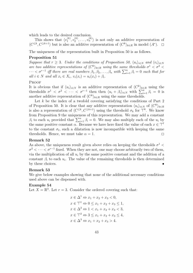
which leads to the desired conclusion.This shows that 〈v(k)

1 , v(k)2 , . . . , v

(k)n 〉 is not only an additive representation of

〈C≤k, C≥k+1〉 but is also an additive representation of 〈Ck〉k∈R in model (A∗). 2

The uniqueness of the representation built in Proposition 50 is as follows.Proposition 51Suppose that r ≥ 3. Under the conditions of Proposition 50, 〈ui〉i∈N and 〈vi〉i∈Nare two additive representations of 〈Ck〉k∈R using the same thresholds σ1 < σ2 <· · · < σr−1 iff there are real numbers β1, β2, . . . , βn with

∑ni=1 βi = 0 such that for

all i ∈ N and all xi ∈ Xi, vi(xi) = ui(xi) + βi.ProofIt is obvious that if 〈ui〉i∈N is an additive representation of 〈Ck〉k∈R using thethresholds σ1 < σ2 < · · · < σr−1 then then 〈ui + βi〉i∈N with

∑ni=1 βi = 0 is

another additive representation of 〈Ck〉k∈R using the same thresholds.Let k be the index of a twofold covering satisfying the conditions of Part 2

of Proposition 50. It is clear that any additive representation 〈ui〉i∈N of 〈Ck〉k∈Ris also a representation of 〈C≤k, C≥k+1〉 using the threshold σk for �k. We knowfrom Proposition 9 the uniqueness of this representation. We may add a constantβi to each ui provided that

∑ni=1 βi = 0. We may also multiply each of the ui by

the same positive constant α. Because we have here fixed the value of each x ∈ �`

to the constant σ`, such a dilatation is now incompatible with keeping the samethresholds. Hence, we must take α = 1. 2

Remark 52As above, the uniqueness result given above relies on keeping the thresholds σ1 <σ2 < · · · < σr−1 fixed. When they are not, one may choose arbitrarily two of them,via the multiplication of all ui by the same positive constant and the addition of aconstant βi to each ui. The value of the remaining thresholds is then determinedby these choices. •Remark 53We give below examples showing that none of the additional necessary conditionsused above can be dispensed with.Example 54Let X = R3. Let r = 3. Consider the ordered covering such that:

x ∈ ∆1 ⇔ x1 + x2 + x3 < 0,

x ∈ �1 ⇔ 0 ≤ x1 + x2 + x3 ≤ 1,

x ∈ ∆2 ⇔ 1 < x1 + x2 + x3 < 3,

x ∈ �2 ⇔ 3 ≤ x1 + x2 + x3 ≤ 4,

x ∈ ∆3 ⇔ x1 + x2 + x3 > 4.

43

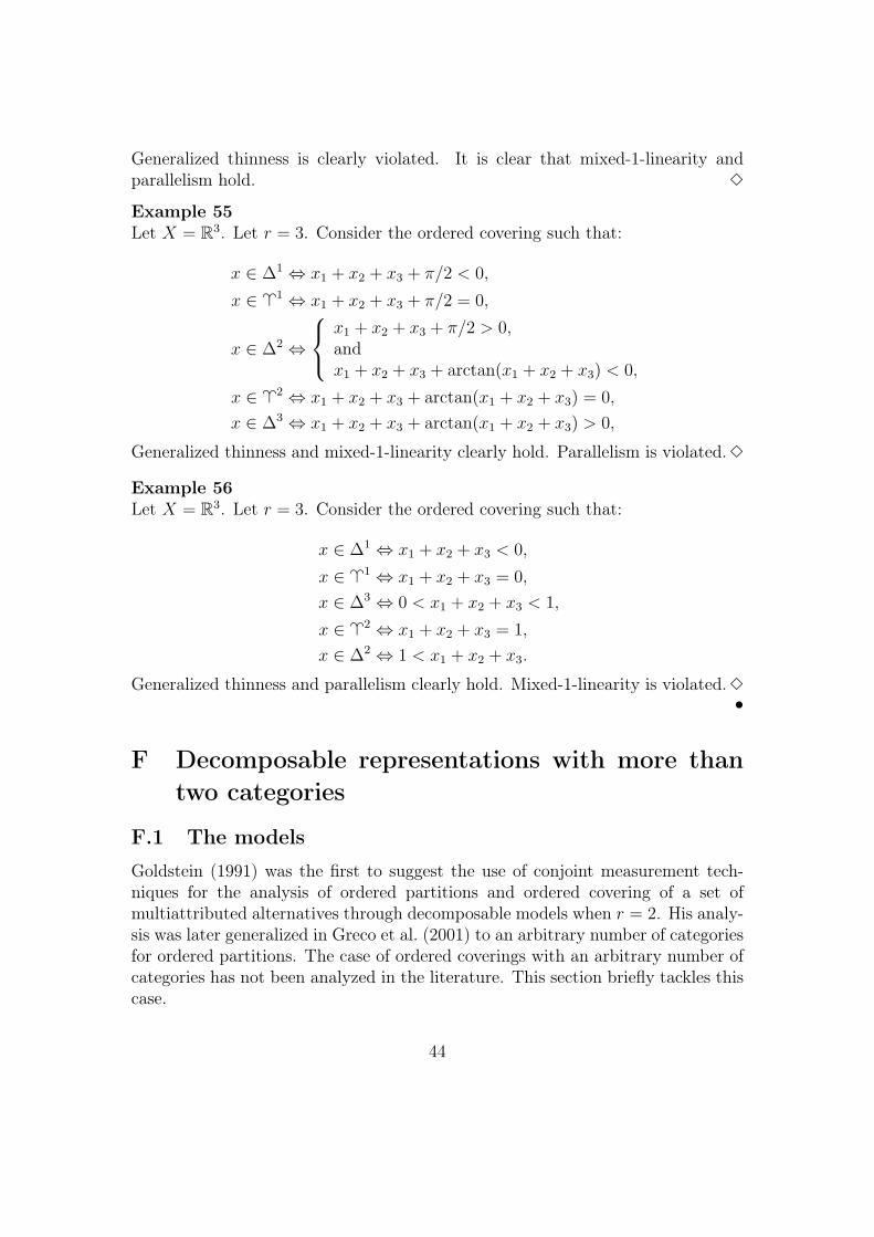
Generalized thinness is clearly violated. It is clear that mixed-1-linearity andparallelism hold. 3

Example 55Let X = R3. Let r = 3. Consider the ordered covering such that:

x ∈ ∆1 ⇔ x1 + x2 + x3 + π/2 < 0,

x ∈ �1 ⇔ x1 + x2 + x3 + π/2 = 0,

x ∈ ∆2 ⇔

x1 + x2 + x3 + π/2 > 0,andx1 + x2 + x3 + arctan(x1 + x2 + x3) < 0,

x ∈ �2 ⇔ x1 + x2 + x3 + arctan(x1 + x2 + x3) = 0,

x ∈ ∆3 ⇔ x1 + x2 + x3 + arctan(x1 + x2 + x3) > 0,

Generalized thinness and mixed-1-linearity clearly hold. Parallelism is violated.3

Example 56Let X = R3. Let r = 3. Consider the ordered covering such that:

x ∈ ∆1 ⇔ x1 + x2 + x3 < 0,

x ∈ �1 ⇔ x1 + x2 + x3 = 0,

x ∈ ∆3 ⇔ 0 < x1 + x2 + x3 < 1,

x ∈ �2 ⇔ x1 + x2 + x3 = 1,

x ∈ ∆2 ⇔ 1 < x1 + x2 + x3.

Generalized thinness and parallelism clearly hold. Mixed-1-linearity is violated.3•

F Decomposable representations with more thantwo categories

F.1 The models

Goldstein (1991) was the first to suggest the use of conjoint measurement tech-niques for the analysis of ordered partitions and ordered covering of a set ofmultiattributed alternatives through decomposable models when r = 2. His analy-sis was later generalized in Greco et al. (2001) to an arbitrary number of categoriesfor ordered partitions. The case of ordered coverings with an arbitrary number ofcategories has not been analyzed in the literature. This section briefly tackles thiscase.

44

Let 〈Ck〉k∈R be an ordered covering of X. We will be interested in conditionsallowing to represent this ordered covering in such a way that, for all x ∈ X andall k ∈ R,

x ∈ Ck ⇔ σk−1 ≤ F (u1(x1), u2(x2), . . . , un(xn)) ≤ σk, (M0)

with the convention that σ0 = −∞, σr = +∞ and where σ1, σ2, . . . , σr−1 are realnumbers such that σ1 < σ2 < · · · < σr−1, ui is a real-valued function on Xi and Fis a real-valued function on

∏ni=1 ui(Xi) that is nondecreasing in all its arguments.

The special case of model (M0) in which the function F is supposed to beincreasing in all its arguments is called model (M1).

In model (M0), we clearly have, for all k ∈ R,

x ∈ �k ⇔ F (u1(x1), u2(x2), . . . , un(xn)) = σk,

x ∈ ∆k ⇔ σk−1 < F (u1(x1), u2(x2), . . . , un(xn)) < σk,

(using the convention adopted above, we have �r = ∅). When F is only supposedto be nondecreasing in each of its arguments, the fact that alternatives lying onthe frontier between two categories have a precise value for F will not be much ofa constraint. Clearly, the situation changes in model (M1). The increasingness ofF will then imply that the frontiers have to be “thin”.

F.2 Model (M0)

Define on each Xi the binary relation %Ri letting, for all xi, yi ∈ Xi,

xi %Ri yi ⇔

for all a−i ∈ X−i and all k ∈ R∗,{

(yi, a−i) ∈ Ck ⇒ (xi, a−i) ∈ C≥k,(yi, a−i) ∈ ∆k ⇒ (xi, a−i) ∈ ∆≥k.

}We use �Ri and ∼Ri as is usual. It is not difficult to see that %R

i is always reflexiveand transitive. When xi %R

i yi, any alternative (xi, a−i) must belong to a cate-gory that is at least as good as the category containing the alternative (yi, a−i).Furthermore, if (yi, a−i) does not lie on the frontier with the category below, thesame will be true with (xi, a−i). Hence, %R

i may be interpreted as an “at least asgood as” relation induced on Xi by the partition 〈Ck〉k∈R. We have:

Lemma 57For all k ∈ R∗ and all x, y ∈ X,

1. [y ∈ Ck and xi %Ri yi] ⇒ (xi, y−i) ∈ C≥k,

2. [y ∈ ∆k and xi %Ri yi] ⇒ (xi, y−i) ∈ ∆≥k,

45

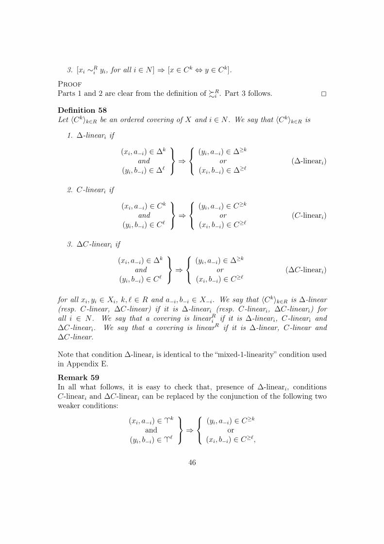
3. [xi ∼Ri yi, for all i ∈ N ] ⇒ [x ∈ Ck ⇔ y ∈ Ck].

ProofParts 1 and 2 are clear from the definition of %R

i . Part 3 follows. 2

Definition 58Let 〈Ck〉k∈R be an ordered covering of X and i ∈ N . We say that 〈Ck〉k∈R is

1. ∆-lineari if

(xi, a−i) ∈ ∆k

and(yi, b−i) ∈ ∆`

⇒

(yi, a−i) ∈ ∆≥k

or(xi, b−i) ∈ ∆≥`

(∆-lineari)

2. C-lineari if

(xi, a−i) ∈ Ck

and(yi, b−i) ∈ C`

⇒

(yi, a−i) ∈ C≥kor

(xi, b−i) ∈ C≥`(C-lineari)

3. ∆C-lineari if

(xi, a−i) ∈ ∆k

and(yi, b−i) ∈ C`

⇒

(yi, a−i) ∈ ∆≥k

or(xi, b−i) ∈ C≥`

(∆C-lineari)

for all xi, yi ∈ Xi, k, ` ∈ R and a−i, b−i ∈ X−i. We say that 〈Ck〉k∈R is ∆-linear(resp. C-linear, ∆C-linear) if it is ∆-lineari (resp. C-lineari, ∆C-lineari) forall i ∈ N . We say that a covering is linearRi if it is ∆-lineari, C-lineari and∆C-lineari. We say that a covering is linearR if it is ∆-linear, C-linear and∆C-linear.

Note that condition ∆-lineari is identical to the “mixed-1-linearity” condition usedin Appendix E.

Remark 59In all what follows, it is easy to check that, presence of ∆-lineari, conditionsC-lineari and ∆C-lineari can be replaced by the conjunction of the following twoweaker conditions:

(xi, a−i) ∈ �k

and(yi, b−i) ∈ �`

⇒

(yi, a−i) ∈ C≥kor

(xi, b−i) ∈ C≥`,

46

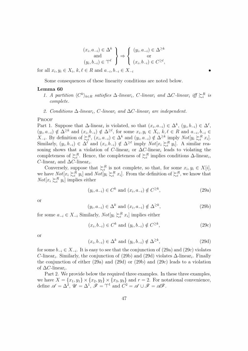
(xi, a−i) ∈ ∆k

and(yi, b−i) ∈ �`

⇒

(yi, a−i) ∈ ∆≥k

or(xi, b−i) ∈ C≥`,

for all xi, yi ∈ Xi, k, ` ∈ R and a−i, b−i ∈ X−i •

Some consequences of these linearity conditions are noted below.

Lemma 601. A partition 〈Ck〉k∈R satisfies ∆-lineari, C-lineari and ∆C-lineari iff %R

i iscomplete.

2. Conditions ∆-lineari, C-lineari and ∆C-lineari are independent.

ProofPart 1. Suppose that ∆-lineari is violated, so that (xi, a−i) ∈ ∆k, (yi, b−i) ∈ ∆`,(yi, a−i) /∈ ∆≥k and (xi, b−i) /∈ ∆≥`, for some xi, yi ∈ Xi, k, ` ∈ R and a−i, b−i ∈X−i. By definition of %R

i , (xi, a−i) ∈ ∆k and (yi, a−i) /∈ ∆≥k imply Not [yi %Ri xi].

Similarly, (yi, b−i) ∈ ∆` and (xi, b−i) /∈ ∆≥` imply Not [xi %Ri yi]. A similar rea-

soning shows that a violation of C-lineari or ∆C-lineari leads to violating thecompleteness of %R

i . Hence, the completeness of %Ri implies conditions ∆-lineari,

C-lineari and ∆C-lineari.Conversely, suppose that %R

i is not complete, so that, for some xi, yi ∈ X[i],we have Not [xi %R

i yi] and Not [yi %Ri xi]. From the definition of %R

i , we know thatNot [xi %R

i yi] implies either

(yi, a−i) ∈ Ck and (xi, a−i) /∈ C≥k, (29a)

or(yi, a−i) ∈ ∆k and (xi, a−i) /∈ ∆≥k, (29b)

for some a−i ∈ X−i Similarly, Not [yi %Ri xi] implies either

(xi, b−i) ∈ Ck and (yi, b−i) /∈ C≥k, (29c)

or(xi, b−i) ∈ ∆k and (yi, b−i) /∈ ∆≥k, (29d)

for some b−i ∈ X−i. It is easy to see that the conjunction of (29a) and (29c) violatesC-lineari. Similarly, the conjunction of (29b) and (29d) violates ∆-lineari. Finallythe conjunction of either (29a) and (29d) or (29b) and (29c) leads to a violationof ∆C-lineari.

Part 2. We provide below the required three examples. In these three examples,we have X = {x1, y1}× {x2, y2}× {x3, y3} and r = 2. For notational convenience,define A = ∆2, U = ∆1, F = �1 and C2 = A ∪F = AF .

47

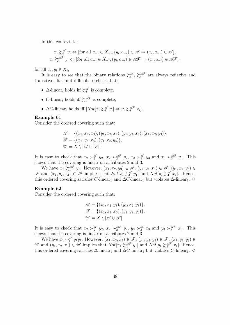
In this context, let

xi %Ai yi ⇔ [for all a−i ∈ X−i, (yi, a−i) ∈ A ⇒ (xi, a−i) ∈ A ] ,

xi %AFi yi ⇔ [for all a−i ∈ X−i, (yi, a−i) ∈ AF ⇒ (xi, a−i) ∈ AF ] ,

for all xi, yi ∈ Xi,It is easy to see that the binary relations %A

i , %AFi are always reflexive and

transitive. It is not difficult to check that:

• ∆-lineari holds iff %Ai is complete,

• C-lineari holds iff %AFi is complete,

• ∆C-lineari holds iff [Not [xi %Ai yi]⇒ yi %AF

i xi].

Example 61Consider the ordered covering such that:

A = {(x1, x2, x3), (y1, x2, x3), (y1, y2, x3), (x1, x2, y3)},F = {(x1, y2, x3), (y1, x2, y3)},U = X \ [A ∪F ].

It is easy to check that x2 �A2 y2, x2 �AF

2 y2, x3 �A3 y3 and x3 �AF

3 y3. Thisshows that the covering is linear on attributes 2 and 3.

We have x1 %AF1 y1. However, (x1, x2, y3) ∈ A , (y1, y2, x3) ∈ A , (y1, x2, y3) ∈

F and (x1, y2, x3) ∈ F implies that Not [x1 %A1 y1] and Not [y1 %A

1 x1]. Hence,this ordered covering satisfies C-linear1 and ∆C-linear1 but violates ∆-linear1. 3

Example 62Consider the ordered covering such that:

A = {(x1, x2, y3), (y1, x2, y3)},F = {(x1, x2, x3), (y1, y2, y3)},U = X \ [A ∪F ].

It is easy to check that x2 �A2 y2, x2 �AF

2 y2, y3 �A3 x3 and y3 �AF

3 x3. Thisshows that the covering is linear on attributes 2 and 3.

We have x1 ∼A1 y1y1. However, (x1, x2, x3) ∈ F , (y1, y2, y3) ∈ F , (x1, y2, y3) ∈

U and (y1, x2, x3) ∈ U implies that Not [x1 %AF1 y1] and Not [y1 %AF

1 x1]. Hence,this ordered covering satisfies ∆-linear1 and ∆C-linear1 but violates C-linear1. 3

48

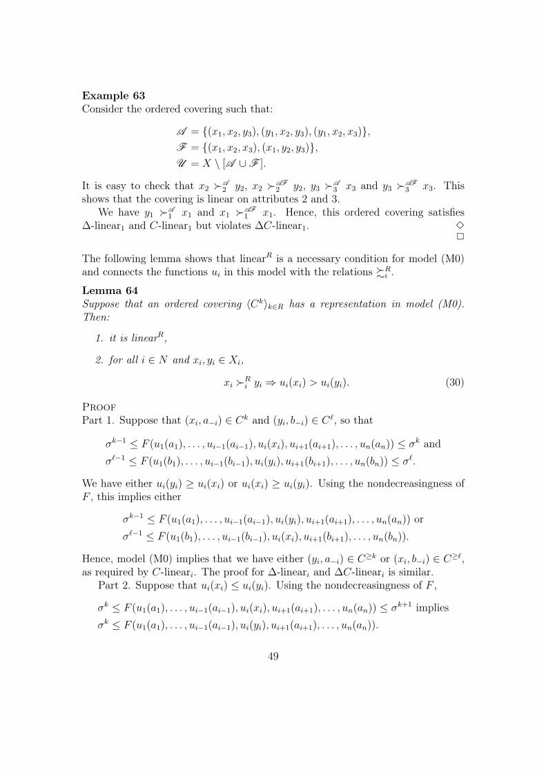
Example 63Consider the ordered covering such that:

A = {(x1, x2, y3), (y1, x2, y3), (y1, x2, x3)},F = {(x1, x2, x3), (x1, y2, y3)},U = X \ [A ∪F ].

It is easy to check that x2 �A2 y2, x2 �AF

2 y2, y3 �A3 x3 and y3 �AF

3 x3. Thisshows that the covering is linear on attributes 2 and 3.

We have y1 �A1 x1 and x1 �AF

1 x1. Hence, this ordered covering satisfies∆-linear1 and C-linear1 but violates ∆C-linear1. 3

2

The following lemma shows that linearR is a necessary condition for model (M0)and connects the functions ui in this model with the relations %R

i .

Lemma 64Suppose that an ordered covering 〈Ck〉k∈R has a representation in model (M0).Then:

1. it is linearR,

2. for all i ∈ N and xi, yi ∈ Xi,

xi �Ri yi ⇒ ui(xi) > ui(yi). (30)

ProofPart 1. Suppose that (xi, a−i) ∈ Ck and (yi, b−i) ∈ C`, so that

σk−1 ≤ F (u1(a1), . . . , ui−1(ai−1), ui(xi), ui+1(ai+1), . . . , un(an)) ≤ σk andσ`−1 ≤ F (u1(b1), . . . , ui−1(bi−1), ui(yi), ui+1(bi+1), . . . , un(bn)) ≤ σ`.

We have either ui(yi) ≥ ui(xi) or ui(xi) ≥ ui(yi). Using the nondecreasingness ofF , this implies either

σk−1 ≤ F (u1(a1), . . . , ui−1(ai−1), ui(yi), ui+1(ai+1), . . . , un(an)) orσ`−1 ≤ F (u1(b1), . . . , ui−1(bi−1), ui(xi), ui+1(bi+1), . . . , un(bn)).

Hence, model (M0) implies that we have either (yi, a−i) ∈ C≥k or (xi, b−i) ∈ C≥`,as required by C-lineari. The proof for ∆-lineari and ∆C-lineari is similar.

Part 2. Suppose that ui(xi) ≤ ui(yi). Using the nondecreasingness of F ,

σk ≤ F (u1(a1), . . . , ui−1(ai−1), ui(xi), ui+1(ai+1), . . . , un(an)) ≤ σk+1 impliesσk ≤ F (u1(a1), . . . , ui−1(ai−1), ui(yi), ui+1(ai+1), . . . , un(an)).

49

Similarly, we have

σk < F (u1(a1), . . . , ui−1(ai−1), ui(xi), ui+1(ai+1), . . . , un(an)) ≤ σk+1 impliesσk < F (u1(a1), . . . , ui−1(ai−1), ui(yi), ui+1(ai+1), . . . , un(an)).

This shows that, for all a−i ∈ X−i, (xi, a−i) ∈ Ck implies (yi, a−i) ∈ C≥k and(xi, a−i) ∈ ∆k implies (yi, a−i) ∈ ∆≥k, so that yi %R

i xi. 2

Omitting the cumbersome formulation of the order-denseness condition in termsof the partition 〈Ck〉k∈R, this leads to:

Proposition 65An ordered covering 〈Ck〉k∈R has a representation in model (M0) iff it is linearR

and, for all i ∈ N , there is a finite or countably infinite set X ′i ⊆ Xi that is densein Xi for %R

i .

ProofThe necessity of linearity follows from Part 1 of Lemma 64. Using Part 2 ofLemma 64, we know that the the weak order induced on Xi by ui always refines%Ri . Hence, there is a finite or countably infinite set X ′i ⊆ Xi that is dense in Xi

for %Ri .

Sufficiency. Using Part 1 of Lemma 60, we know that %Ri is a weak order.

Since there is a finite or countably infinite set X ′i ⊆ Xi that is dense in Xi for %Ri ,

there is a real-valued function ui on Xi such that, for all xi, yi ∈ Xi,

xi %Ri yi ⇔ ui(xi) ≥ ui(yi). (31)

Consider, on each i ∈ N any function ui satisfying (31) and take any σ0, σ1,. . . , σr ∈ R such that σ0 < σ1 < · · · < σr. For all k ∈ {1, 2, . . . r}, consider anyincreasing function φk mapping R into (σk−1, σk). Define F on

∏ni=1 ui(Xi) letting,

for all x ∈ X and all k ∈ R,

F (u1(x1), u2(x2), . . . , un(xn)) =

{φk (∑n

i=1 ui(xi)) if x ∈ ∆k,

σk if x ∈ �k.(32)

The well-definedness of F follows from Part 3 of Lemma 57 together with (31). Itsnondecreasingness is easily shown using the definition of ui and Parts 1 and 2 ofLemma 57. 2

The above proposition generalizes Part 3 of Theorem 1 in Goldstein (1991, p. 70)to the case of an arbitrary number of category.

50

Remark 66The uniqueness of the representation in model (M0) is easily analyzed. Observefirst that the thresholds σ2, σ3, . . . , σr−1 maybe be chosen arbitrarily provided thatthey satisfy:

σ2 < σ3 < . . . , < σr−1. (33)

Part 2 of Lemma 64 has shown that in all representations of 〈Ck〉k∈R in model (M0),ui must satisfy (30). Consider, independently on each attribute any function uisatisfying (30). For k = 2, 3, . . . , r − 1, consider any function fk from Rn into(σk−1, σk) being nondecreasing in each of its arguments. Take any function f1

(resp. fr) from Rn into (−∞, σ1) (resp. (σr−1,+∞) that is nondecreasing in eachof its arguments. Define the function the real-valued F on

∏ni=1 ui(Xi) letting, for

all x ∈ X,

F (u1(x1), . . . , un(xn)) =

{fk(u1(x1), . . . , un(xn)) if x ∈ ∆k,

σk if x ∈ �k.(34)

It is clear that this defines a representation of 〈Ck〉k∈R in model (M0). It isnot difficult to see that only such representations may be used. Therefore, thecombination of (30), (33), and (34) describe the set of all representations of 〈Ck〉k∈Rin model (M0). •

F.3 Model (M1)

Since model (M0) only requires the function F to be nondecreasing, it should beapparent that this model does not deal with alternatives at the frontier betweentwo categories in a special way. Things change with model (M1) that requires F tobe increasing in all its arguments. This motivates the introduction of the followingcondition.

Definition 67We say that the covering 〈Ck〉k∈R satisfies thinRi if,

(xi, a−i) ∈ �k

and(yi, a−i) ∈ �k

⇒ [(xi, b−i) ∈ C` ⇔ (yi, b−i) ∈ C`

]for all xi, yi ∈ Xi, k, ` ∈ R and a−i, b−i ∈ X−i. We say that 〈Ck〉k∈R is thinR ifsatisfies thinRi on all attributes i ∈ N .

This condition is identical to the condition called in “Generalized 1-thinness” inAppendix E. Intuitively, a covering satisfies thinRi if, as soon as two distinct levelson Xi are caught in a frontier when they are associated with the same evaluations

51

on the attributes other than i, it will be impossible for these two levels to bedistinguished, i.e., they will be linked by ∼Ri . It is easy to see that thinRi is anecessary condition for model (M1). Indeed, the premise of thinRi implies that:

F (u1(a1), . . . , ui−1(ai−1), ui(xi), ui+1(ai+1), . . . , un(an)) =

F (u1(a1), . . . , ui−1(ai−1), ui(yi), ui+1(ai+1), . . . , un(an)).

Because F is increasing, this can only happen if ui(xi) = ui(yi), which leads to thedesired conclusion.

The following lemma takes note of some important consequences of thinnesswhen combined with linearity.

Lemma 681. Suppose that 〈Ck〉k∈R satisfies linearRi and thinRi on attribute i ∈ N . Then

[(xi, a−i) ∈ �k and yi �Ri xi]⇒ (xi, a−i) ∈ ∆≥k,

[(xi, a−i) ∈ �k and xi �Ri zi]⇒ (zi, a−i) /∈ ∆≥k.

for all xi, yi, zi ∈ Xi, k ∈ R∗ and a−i ∈ X−i.

2. Conditions ∆-lineari, C-lineari, ∆C-lineari and thinRi are independent.

ProofPart 1. Suppose that (xi, a−i) ∈ �k and yi �Ri xi. Because yi %R

i xi, we knowthat (yi, a−i) ∈ C≥k. Suppose that (yi, a−i) ∈ �k. Using thinRi , (xi, a−i) ∈ �k and(yi, a−i) ∈ �k imply xi ∼Ri yi, a contradiction. The proof of the other implicationis similar.

Part 2. It is easy to check that in Examples 61, 62 and 63 the covering con-sidered satisfy thinR. We give below the remaining example, using notation intro-duced before Example 61.

Example 69Consider the ordered covering such that:

A = {(x1, x2, x3), (x1, y2, x3), (y1, x2, x3)},F = {(x1, x2, y3), (y1, x2, y3)},

U = X \ [A ∪F ].

Conditions thinR2 and thinR3 are trivially satisfied. Condition thinR1 is violated since(x1, x2, y3) ∈ F and (y1, x2, y3) ∈ F , (x1, y2, x3) ∈ A and (y1, y2, x3) ∈ U . It issimple to check that we have xi �A

i yi and xi �AFi yi, for all i ∈ N , which show

that the covering satisfies linearR. 32

52

The following proposition generalizes Part 4 of Theorem 1 in Goldstein (1991, p.70) to the case of an arbitrary number of category.

Proposition 70A covering 〈Ck〉k∈R has a representation in model (M1) iff it satisfies linearR,thinR and, for all i ∈ N , there is a finite or countably infinite set X ′i ⊆ Xi that isdense in Xi for %R

i .

ProofNecessity. Since model (M1) implies model (M0), the necessity of linearity and theorder-denseness conditions follows from Proposition 65. The necessity of thinnesswas shown above.

Sufficiency. Define ui and F as in the proof of Proposition 65. The well-definedness of F follows from Part 3 of Lemma 57 together with (31). Supposethat ui(xi) > ui(yi), so that xi �Ri yi. If (yi, a−i) ∈ ∆k, for some k ∈ R, Part 3of Lemma 57 implies that (yi, a−i) ∈ ∆≥k. The conclusion therefore follows fromthe definition of F . If (yi, a−i) ∈ �k, for some k ∈ R, Part 1 of Lemma 68 impliesthat (xi, a−i) ∈ ∆≥k. The conclusion therefore follows from the definition of F . 2

Remark 71The uniqueness of the representation in model (M1) is only slightly stronger thanwhat was the case with model (M0). It is first clear that the thresholds can bechosen arbitrarily provided that they satisfy (33). Similarly, the functions ui mustsatisfy (30). If, for some xi, yi ∈ Xi and some a−i ∈ X−i, we have (xi, a−i) ∈ �k

and (yi, a−i) ∈ �k, for some k ∈ R, model (M1) implies that we must haveui(xi) = ui(yi). It is not difficult to see that these are the only constraints on ui.Therefore, we may, independently on each attribute i ∈ N , choose any function uisuch that, for all xi, yi ∈ Xi,

xi �Ri yi ⇒ ui(xi) > ui(yi),

(xi, a−i) ∈ �k and (yi, a−i) ∈ �k, for some k ∈ R,⇒ ui(xi) = ui(yi).(35)

For k = 2, 3, . . . , r − 1, consider any function fk from Rn into (σk−1, σk) beingincreasing in each of its arguments. Take any function f1 (resp. fr) from Rn into(−∞, σ1) (resp. (σr−1,+∞) that is increasing in each of its arguments. Define thefunction using (34). It is easy to see that this leads to representation of 〈Ck〉k∈Rin model (M1) and that only such representations may be used. •

Consider an ordered covering 〈Ck〉k∈R such that, for all k ∈ R, �k = ∅, i.e., anordered partition. This implies that, for all k ∈ R, Ck = ∆k and C≥k = ∆≥k. It isthen easy to see that, for all i ∈ N , conditions ∆-lineari, C-lineari and ∆C-linearibecome equivalent. Furthermore, condition thinRi is always trivially satisfied. Thisallows to state the following corollary of Propositions 65 and 70.

53

Proposition 72Let 〈Ck〉k∈R be an ordered partition of X. There are real numbers σ0 < σ1 <· · · < σr and real-valued functions ui on Xi and F on

∏ni=1 ui(Xi) with F being

increasing in all its arguments such that, for all x ∈ X and all k ∈ R,

x ∈ Ck ⇔ σk−1 < F (u1(x1), u2(x2), . . . , un(xn)) < σk, (36)

iff 〈Ck〉k∈R is ∆-linear and, for all i ∈ N there is a finite or countably infinite setX ′i ⊆ Xi that is dense in Xi for %R

i .

This proposition generalizes Theorem 2 in Goldstein (1991, p. 72) to the case ofan arbitrary number of category. Greco et al. (2001) and Słowiński et al. (2002)state a version of this result when X is finite or countably infinite. Bouyssou andMarchant (2007b) have given a direct proof of Proposition 72. It is easy to seethat for an ordered partition, there is a representation (36) with F increasing inall its arguments iff there is a representation (36) with F nondecreasing in all itsarguments. Again, the distinction between increasingness and nondecreasingnessonly matters if there are alternatives at the frontier between categories.

F.4 Extensions

In the r = 2 case, Goldstein (1991) has suggested two weaker forms of model (M0)and has given a complete characterization of these two variants. It is not difficultto extend this analysis to the general case.

The weakest form, called model (M), is obtained from model (M0) by removingthe requirement that F is nondecreasing in each of its arguments. It is easyto characterize this model. Remember that the relation ∼Ri is an equivalence.Suppose that model (M) holds and that Not [xi ∼Ri yi]. This clearly implies thatwe must have ui(xi) 6= ui(yi). Since ui is real-valued, this implies that theremust exist a one-to-one correspondence between Xi/∼Ri and some subset of R.Conversely, suppose that this condition is satisfied, for all i ∈ N . This impliesthat, for all i ∈ N , there is a real-valued function ui such that

xi ∼Ri yi ⇔ ui(xi) = ui(yi). (37)

Take on each attribute i ∈ N any function ui satisfying (37) and define F asin the proof of Proposition 65. The well-definedness of F follows from Part 3 ofLemma 57 together with (37). This shows that as soon as the cardinality of Xi/∼Riis not too large, all ordered coverings have a representation in model (M).

Another variant of model (M0), called model (M′) is obtained replacing the factthat F is nondecreasing in each of its arguments by the fact that F is one-to-one

54

in each of its arguments, i.e., is such that for all i ∈ N and all αi, βi, γi ∈ ui(Xi),

F (α1, . . . , αi−1, βi, αi+1, . . . , αn) =

F (α1, . . . , αi−1, γi, αi+1, . . . , αn)

}⇒ βi = γi.

Because model (M′) implies model (M), we know that, for all i ∈ N , there mustexist a one-to-one correspondence between Xi/∼Ri and some subset of R. Moreimportantly, this model implies condition thinRi , for all i ∈ N . Indeed suppose that(xi, a−i) ∈ �k and (yi, a−i) ∈ �k. This implies, abusing notation in an obviousway, F (ui(xi),K) = F (ui(yi),K) = σk. Using one-to-one decomposability impliesui(xi) = ui(yi), so that, for all ` ∈ R and b−i ∈ X−i, (xi, b−i) ∈ C` ⇔ (yi, b−i) ∈ C`.

Conversely, let us show that as soon as an ordered covering is thin and satisfiesthe order-denseness condition, it has a representation in model (M′). Using theorder-denseness condition, choose on each Xi a real-valued function satisfying (37)and define F as in the proof of Proposition 65. It remains to show that such afunction F is one-to-one in each variable. Suppose that

F (u1(a1), . . . , ui−1(ai−1), ui(xi), ui+1(ai+1), . . . , un(an)) =

F (u1(a1), . . . , ui−1(ai−1), ui(yi), ui+1(ai+1), . . . , un(an)) = λ.

If λ /∈ {σ0, σ1, . . . , σr}, the definition of F implies that ui(xi) = ui(yi). If λ ∈{σ0, σ1, . . . , σr}, we have (xi, a−i) ∈ �k and (yi, a−i) ∈ �k. Therefore, conditionthinRi implies xi ∼Ri yi, so that ui(xi) = ui(yi).

The uniqueness of the representations in models (M) and (M′) is obviouslyextremely weak. It can be easily analyzed along the lines sketched in Bouyssouand Marchant (2007a).

ReferencesBelton, V. and Stewart, T. (2001). Multiple criteria decision analysis: An integrated

approach. Kluwer, Dordrecht.Bouyssou, D. (1986). Some remarks on the notion of compensation in MCDM. European

Journal of Operational Research, 26:150–160.Bouyssou, D. and Marchant, Th. (2007a). An axiomatic approach to noncompensa-

tory sorting methods in MCDM, I: The case of two categories. European Journal ofOperational Research, 178(1):217–245.

Bouyssou, D. and Marchant, Th. (2007b). An axiomatic approach to noncompensa-tory sorting methods in MCDM, II: More than two categories. European Journal ofOperational Research, 178(1):246–276.

Bouyssou, D. and Marchant, Th. (2008a). Additive conjoint measurement with orderedcategories: A theoretical look at some sorting methods in MCDM. Working paper,LAMSADE, Université Paris Dauphine.

55

Bouyssou, D. and Marchant, Th. (2008b). Biorders and bi-semiorders with frontiers.Working paper, LAMSADE, Université Paris Dauphine.

Bouyssou, D. and Marchant, Th. (2008c). Ordered categories and additive conjoint mea-surement on connected sets. Working paper, LAMSADE, Université Paris Dauphine,Paris.

Bouyssou, D., Marchant, Th., Pirlot, M., Tsoukiàs, A., and Vincke, Ph. (2006). Evalua-tion and decision models: Stepping stones for the analyst. Springer, New York.

Chateauneuf, A. and Wakker, P. P. (1993). From local to global additive representation.Journal of Mathematical Economics, 22(6):523–545.

Doignon, J.-P., Ducamp, A., and Falmagne, J.-C. (1984). On realizable biorders and thebiorder dimension of a relation. Journal of Mathematical Psychology, 28:73–109.

Doignon, J.-P., Ducamp, A., and Falmagne, J.-C. (1987). On the separation of tworelations by a biorder or a semiorder. Mathematical Social Sciences, 13:1–18.

Doumpos, M. and Zopounidis, C. (2002). On the development of an outranking relationfor ordinal classification problems: An experimental investigation of a new methodol-ogy. Optimization Methods ad Software, 17:293–317.

Doumpos, M. and Zopounidis, C. (2004). A multicriteria classification approach basedon pairwise comparisons. European Journal of Operational Research, 158:378–389.

Ducamp, A. and Falmagne, J.-C. (1969). Composite measurement. Journal of Mathe-matical Psychology, 6:359–390.

Figueira, J., De Smet, Y., and Brans, J.-P. (2004). MCDA methods for sorting andclustering problems: PROMETHEE TRI and PROMETHEE CLUSTER. Researchreport, SMG - ULB.

Fishburn, P. C. (1970). Utility theory for decision-making. Wiley, New York.Fishburn, P. C. (1991). Nontransitive additive conjoint measurement. Journal of Math-

ematical Psychology, 35:1–40.Fishburn, P. C. (1992). On nonstandard nontransitive additive utility. Journal of Eco-

nomic Theory, 56:426–433.Fishburn, P. C. (1997). Cancellation conditions for multiattribute preferences on finite

sets. In: M. H. Karwan, J. Spronk, and J. Wallenius (Eds.) Essays in Decision Making,pp. 157–167. Springer-Verlag, Berlin.

Fishburn, P. C. (2001). Cancellation conditions for finite two-dimensional additive mea-surement. Journal of Mathematical Psychology, 45:2–26.

Fishburn, P. C., Lagarias, J. C., Reeds, J. A., and Shepp, L. A. (1991). Sets uniquelydetermined by projections on axes II: Discrete case. Discrete Mathematics, 91:149–159.

Fishburn, P. C. and Shepp, L. A. (1999). Sets of uniqueness and additivity in integerlattices. In: G. T. Herman and A. Kuba (Eds.) Discrete tomography. Foundations,Algorithms, Applications, pp. 35–58. Birkhäuser, Boston.

Goldstein, W. M. (1991). Decomposable threshold models. Journal of MathematicalPsychology, 35:64–79.

Greco, S., Matarazzo, B., and Słowiński, R. (1999). The use of rough sets and fuzzy

56

sets in MCDM. In: T. Gal, T. Hanne, and T. Stewart (Eds.) Multicriteria decisionmaking, Advances in MCDM models, algorithms, theory and applications, pp. 14.1–14.59. Kluwer, Dordrecht.

Greco, S., Matarazzo, B., and Słowiński, R. (2001). Conjoint measurement and roughset approach for multicriteria sorting problems in presence of ordinal criteria. In:A. Colorni, M. Paruccini, and B. Roy (Eds.) A-MCD-A, Aide Mulcritère à la Décision/ Multiple Criteria Decision Aid, pp. 117–144. European Commission, Joint ResearchCentre, Luxembourg.

Greco, S., Matarazzo, B., and Słowiński, R. (2002a). Multicriteria classification. In:W. Klogsen and J. Zytkow (Eds.) Handbook of data mining and knowledge discovery,pp. 318–328. Oxford University Press, Oxford.

Greco, S., Matarazzo, B., and Słowiński, R. (2002b). Rough sets methodology for sortingproblems in presence of multiple attributes and criteria. European Journal of Opera-tional Research, 138:247–59.

Greco, S., Matarazzo, B., and Słowiński, R. (2005). Decision rule approach. In:J. Figueira, S. Greco, and M. Ehrgott (Eds.) Multiple Criteria Decision Analysis:State of the Art Surveys, pp. 507–562. Springer-Verlag, Boston.

Henriet, L. (2000). Systèmes d’évaluation et de classification multicritères pour l’aide àla décision. Construction de modèles et procédures d’affectation. Thèse de doctorat,Université Paris Dauphine, Paris, France. (in French).

Jacquet-Lagrèze, É. (1995). An application of the UTA discriminant model for theevaluation of R&D projects. In: P. Pardalos, Y. Siskos, and C. Zopounidis (Eds.)Advances in Multicriteria Analysis, pp. 203–211. Kluwer, Dordrecht.

Keeney, R. L. and Raiffa, H. (1976). Decisions with multiple objectives: Preferences andvalue tradeoffs. Wiley, New York.

Köksalan, M. and Ulu, C. (2003). An interactive approach for placing alternatives inpreference classes. European Journal of Operational Research, 144:429–439.

Krantz, D. H., Luce, R. D., Suppes, P., and Tversky, A. (1971). Foundations of measure-ment, vol. 1: Additive and polynomial representations. Academic Press, New York.

Levine, M. V. (1970). Transformations that render curves parallel. Journal of Mathe-matical Psychology, 7:410–443.

Marichal, J.-L., Meyer, P., and Roubens, M. (2005). Sorting multi-attribute alternatives:The TOMASO method. Computers & Operations Research, 32:861–877.

Marichal, J.-L. and Roubens, M. (2001). On a sorting procedure in the presence ofqualitative interacting points of view. In: J. Chojean and J. Leski (Eds.) Fuzzy Setsand their Applications, pp. 217–230. Silesian University Press, Gliwice.

Meyer, P and Roubens, M. (2005). Choice, ranking and sorting in fuzzy multiple crite-ria decision aid. In: J. Figueira, S. Greco, and M. Ehrgott (Eds.) Multiple CriteriaDecision Analysis: State of the Art Surveys, pp. 471–506. Springer-Verlag, Boston.

Mousseau, V., Słowiński, R., and Zielniewicz, P. (2000). A user-oriented implementationof the ELECTRE TRI method integrating preference elicitation support. Computers& Operations Research, 27:757–777.

57

Nakamura, Y. (2004). Trichotomic preferences for gambles. Journal of MathematicalPsychology, 48(6):385–398.

Perny, P. (1998). Multicriteria filtering methods based on concordance and non-discordance principles. Annals of Operations Research, 80:137–165.

Roy, B. (1996). Multicriteria methodology for decision aiding. Kluwer, Dordrecht. Orig-inal version in French: “Méthodologie multicritère d’aide à la décision”, Economica,Paris, 1985.

Roy, B. and Bouyssou, D. (1993). Aide multicritère à la décision : méthodes et cas.Economica, Paris.

Scott, D. (1964). Measurement structures and linear inequalities. Journal of Mathemat-ical Psychology, 1:233–247.

Słowiński, R., Greco, S., and Matarazzo, B. (2002). Axiomatization of utility, outrank-ing and decision-rule preference models for multiple-criteria classification problemsunder partial inconsistency with the dominance principle. Control and Cybernetics,31(4):1005–1035.

Vind, K. (1991). Independent preferences. Journal of Mathematical Economics, 20:119–135.

Vind, K. (2003). Independence, Additivity, Uncertainty. Springer-Verlag, Berlin.Wei, Y. (1992). Aide multicritère à la décision dans le cadre de la problématique du tri :

concepts, méthodes et applications. Thèse de doctorat, Université Paris Dauphine,Paris, France. (in French).

Wille, U. (2000). Linear measurement models: Axiomatizations and axiomatizability.Journal of Mathematical Psychology, 44:617–650.

von Winterfeldt, D. and Edwards, W. (1986). Decision analysis and behavioral research.Cambridge University Press, Cambridge.

Zopounidis, C. and Doumpos, M. (2000a). Intelligent decision aiding systems based onmultiple criteria for financial engineering. Kluwer, Dordrecht.

Zopounidis, C. and Doumpos, M. (2000b). PREFDIS: A multicriteria decision supportsystem for sorting decision problems. Computers & Operations Research, 27(7–8):779–797.

Zopounidis, C. and Doumpos, M. (2002). Multicriteria classification and sorting methods:A literature review. European Journal of Operational Research, 138:229–246.

58