"AD-.A279 930

DTICELECTE

JUN Q P

NEURAL NETWORKS FORASSA•A CIF RADAR SIGNALS

by

Christopher A.P. Carter and Nathalie Mass6

94-16305

DEFENCE RESEARCH ESTABLISHMENT OTTAWATECHNICAL NOTE 93-33

r November 1993Ottawa

S/ 031i " •k'' " . . ....I iI | I

Il1*" N"6fnDOftce nam

NEURAL NETWORKS FORCLASSIFICATION OF RADAR SIGNALS

by

Christopher A.P. CarterRadar Electronic Support Measures Section

Electronic Warfare Division

and

Nathalie MasseApplied Silicon Inc. Canada

DEFENCE RESEARCH ESTABLISHMENT OTTAWATECHNICAL NOTE 93-33

PCN November 1993041 LB Ottawa

.AB&FRACT

Radar Electromic Support Measures (ESM) systems are faced with increasingly dense andcomplex electromagtic environments. Traditional algorithms for signal recognition and analysisare highly complex, conputation a ly intensive, often rely on heuristics, and require humans toverify and validate the analysis. In this paper, the use of an alternative technique - artificialneural networks - to classify pulse-to-pulse signal modulation patterns is investigated. Neuralnetworks are an attractive alternative because of their potential to solve difficult classificationproblems mome effectively and more quickly than conventional techniques. Neural networksadapt to a problem by learning, even in the presence of noise or distortion in the input data,without the requirement for human programming. In the paper, the fundamentals of networkconstruction, training, behaviour and methods to improve the training process and enhance anetwork's perfmance are discussed. The results and a description of the classificationexperiments are also presented.

L'envirnnement dlectromagn6tique dans lequel doit op6rer le systbme de Mesure deSoutien Electroniques (MSE) pour signaux radar est de plus en plus dense et complexe. Lesalgorithmes classiques de reconnaissance et de traitement de ces signaux sont complexes etheuristiques; ils requi6rent en gdn~al de longs temps de calcul ainsi que l'intervention humainedana les dtapes d'analyse et de validation. LUs rdseaux de neurones artificiels sont une solutionde rechange int6rssante vu leur capacit6 i rdsoudre des problbnes complexes de classificationde maniare plus efficace et plus rapide que les algorithmes classiques. Leur capacit6 d'apprendreleur permet de s'a4apter an problame meme en environnement bruitd ou pour une distortion desentrdes et ce, sans l'intervention humaine. Dans ce rapport, les riseaux de neurones artificielssont utilisds pour effectuer la classification de signaux selon le type de modulation de lafr~quence des impulsions. Dans la premitre partie du rapport, la structure, les algorithmesd'apprentisage et le com m ent d'un rdseau sont prdsent6s. On aborde Egalement la questionde l'acc•ldration de la vitesse d'apprentissage. La deuxitme partie d6crit les rdsultats desclassifications de signaux effectudes par rdseau de neurones.

Accession For

NTIS GiiiDTIC TAB 0Unannoucced 0]jamstirioution

By

Distribution/'.

Availability Qodes

Avall an/orDist Speooal

EXECUTIVE SUMMARY

The purpose of a radar Electronic Support Measures (ESM) system is to detect, determine

signal parameter values, and identify radar emitters in the electromagnetic environment. Research

initiated at the Defence Research Establishment Ottawa (DREO) has supported the development

of hardware and software for the next generation naval ESM system. This project is called

CANEWS 2.

CANEWS 2 incorporates a number of complex signal processing algorithms designed to

classify radar signals. One of these determines the pulse-to-pulse modulation pattern of an agile

signal. The objective of this paper is to investigate the technology of neural networks and their

applicability to this signal classification problem.

The potential offered by' artificial neiral networks has sparked a great deal of interest in

the research community. Although traditional algorithms have been very successful at tasks that

are characterized by formal logical rules, they have had little success at tasks which are difficult

to characterize this way. These are often tasks that the human brain performs well, such as

pattern recognition and common-sense reasoning. Among the attractive features of neural

networks are their ability to learn, even in the presence of noise or distortion in the input data,

the ease of maintenance, high performance, and the potential to solve difficult classification

problems more effectively than conventional techniques.

The basic component of an artificial network is the artificial neuron. A network is created

by connecting a number of neurons together. Each neuron contributes to the overall function

performed by the network by taking values from the nodes on its input side and calculating a

value which it passes on to the nodes on its output side. A special set of nodes are designated

as initial input nodes; each node receives a single value from a vector representing the

characteristics of an input to the network. These values are transformed as they propagate

through the network - the final destination being a set of nodes designated as the network's

output. The output vector produced by these nodes represents a function of the initial input

vector.

This paper covers the fundamentals of neural network construction, training, and

behaviour, then deals with problems pertaining to a particular type of network called the

v

back-propagadon network. Back-propagation networks are the most commonly used networks

for practical applications. A number of pragmatic considerations in the design of such networks

to improve their learning capacity and to enhance their performance are described. A set of

neural networks to classify signal modulation patterns were initially designed to take the

frequency values from a pulse train as input. By designing new networks, that took input values

to which a Fourier transform had been applied, performance was greatly improved. The results

obtained from these experiments have led the authors to conclude that neural networks are a

promising technology in the area of radar signal classification.

vi

TABLE OF CONTENTS

Page

ABSTRACT ....................................................... iii

EXECUTIVE SUMMARY ............................................. v

TABLE OF CONTENTS ............................................. vii

LIST OF FIGURES ................................................. ix

LIST OF TABLES .................................................. xi

1.0 INTRODUCTION .............................................. 1

1.1 Signal Classification in CANEWS 2 ........................... 1

1.2 Neural Networks ......................................... 2

2.0 THEORY .................................................... 4

2.1 The Artificial Neuron ..................................... 4

2.2 Neural Network Types ..................................... 6

2.3 Training ............................................... 8

2.3.1 Training Algorithms ................................. 8

2.4 Summary .............................................. 9

3.0 BACK-PROPAGATION .......................................... 10

3.1 Background ............................................ 10

3.2 Output Layer Learning Rule ................................. 11

3.3 Hidden Layer Learning Rule ................................. 12

3.4 Internal Behaviour ........................................ 13

3.5 Variations of Back-propagation Training ........................ 14

vii

TABLE OF CONTENTS (cont'd)

page

3.5.1 Varying the Coefficients .............................. 15

3.5.2 The Momentum Method .............................. 15

3.5.3 Cumulative Update of Weights .......................... 15

3.6 Summary .............................................. 16

4.0 PRACTICAL CONSIDERATIONS .................................. 16

4.1 Pre-areatment of Input Data ................................. 16

4.2 Weight Initialization and Adjustment ........................... 18

4.3 Choosing the Number of Training Vectors ....................... 18

4.4 Network Design ......................................... 18

4.4.1 Number of Layers ................................... 19

4.4.2 Number of Modes Per Layer ........................... 19

4.5 Summary .............................................. 20

5.0 CLASSIFICATION OF RADAR SIGNALS ............................ 20

5.1 Time Domain Experiments .................................. 21

5.2 The Frequency Domain .................................... 30

5.2.1 The Fourier Transform ............................... 30

5.2.2 Frequency Domain Experiments ......................... 31

5.3 Observations ............................................ 36

6.0 CONCLUSIONS ............................................... 37

7.0 REFERENCES ................................................ 39

Appendix A ...................................................... A-i

viii.,

LIST OF FIGURES

Page

Figure 1: Structure of an Artificial Neuron . 4

Figure 2: Common Transfer Functions ................................... 5

Figure 3: Network Types (from Handbook of Neural Computing [101) ............ 7

Figure 4: Signal Modulation Patterns .................................... 21

Figure 5: 16-5-5 Results ............................................. A-2

Figure 6: 16-10-5 Results ............................................ A-3

Figure 7: 16-15-5 Results ............................................ A-4

Figure 8: 16-20-5 Results ............................................ A-5

Figure 9: 16-25-5 Results ............................................ A-6

Figure 10 32-5-5 Results ............................................ A-7

Figure 11: 32-10-5 Results ........................................... A-8

Figure 12: 32-15-5 Results ......................................... A-9

Figure 13: 32-20-5 Results .......................................... A-10

Figure 14: 32-25-5 Results .......................................... A-11

Figure 15: 16-4-4 Results ........................................... A-12

Figure 16: 16-8-4 Results ........................................... A-13

Figure 17: 16-12-4 Results .......................................... A-14

Figure 18: 16-16-4 Results ........................................ A-15

Figure 19: 16-20-4 Results .......................................... A-16

Figure 20. 32-4-4 Results ........................................... A-17

Figure 21: 32-8-4 Results ......................................... A-18

Figure 22: 32-12-4 Results .......................................... A-19

Figure 23: 32-16-4 Results .......................................... A-20

Figure 24: 32-20-4 Results .......................................... A-21

ix

LWS OF TABLES

Page

Table I: Time Domain: Number of Training Vectors ........................ 26

Table M: Time Domain: Pulse Count, Period and Phase Settings ................ 27

Table IMI: Tune Domain: Network Results 16 Input Nodes ..................... 28

Table IV: Time Domain: Network Results 32 Input Nodes ..................... 29

Table V: Frequency Domain: Number of Training Vectors .................... 32

Table VI: Frequency Domain: Pulse Count, Period and Phase Settings ............ 33

Table VII: Frequency Domain: Network Results 16 Input Nodes ................ 34

Table VIII: Frequency Domain: Network Results 32 Input Nodes ............... 35

xi

1.0 INTRODUCTION

The purpose of a radar Electronic Support Measures (ESM) system is to detect, determine

signal parameter values, and identify radar emitters in the electromagnetic environment. Research

initiated at the Defence Research Establishment Ottawa (DREO) has supported the development

of hardware and software for the next generation naval ESM system. This project is called

CANEWS 2.

CANEWS 2 incorporates a number of signal processing algorithms designed to classify

radar signals. One of these determines the pulse-to-pulse modulation pattern of an agile signal.

The goal of this paper is to investigate the technology of neural networks and their applicability

to this signal classification problem.

1.1 Signal Classification in CANEWS 2

The approach taken by the CANEWS 2 software to identify radar emitters is to first

deinterleave the detected signals into separate tracks. For an individual track, a classification is

performed on each of the signal's parameters: pulse width, radio frequency of each pulse (RF),

pulse repetition interval (PRI), and scan pattern. The classification process reveals structural and

statistical attributes for each parameter. Identification then finds radars in an emitter library

whose known characteristics match the observed characteristics on a parameter by parameter

basis.

Of particular interest are the algorithms used to determine the structural and statisticai

attributes of the parameters. For each parameter, CANEWS 2 maintains a hierarchy of all of its

possible structural characteristics. Entries at the same level in the taxonomy represent mutually

exclusive classifications, entries below a particular entry represent specializations of that entry.

For example, an RF signal is divided into two mutually exclusive classifications, either pulsed

or continuous wave. Within the pulsed classification are two sub-classifications; the pulses either

maintain a constant frequency or they vary from pulse to pulse. The variable classification in

turn has two sub-classifications; the variation is either periodic or random; and of these structural

possibilities, the signal could either cover an entire range of RF values in a continuous fashion,

or merely cover a range at discrete points.

1

A set of statistical values is maintained for each structural classification. For example,

in the case of a pulsed, variable, periodic, continuous RF signal, the set includes: the limits and

the mean of the RF values observed, a description of the pulse-to-pulse modulation pattern (ramp,

sinusoidal, triangular, ...), and the length of the period of the pattern. In the case of a random

continuous RF signal, the set includes: the limits and mean as before, as well as a description

of the probability distribution of the RF values (Gaussian, uniform, triangular, ...). The

algorithms to compute these values, in particular the pulse-to-pulse modulation pattern and the

probability distribution, have a high order of complexity. To determine the type of the

modulation pattern, a match is made between a normalized set of the observed pulses and a sine

wave to obtain a "goodness of fit" based on heuristics. This process is repeated for the other

possible modulation patterns. The match with the highest goodness of fit determines the

modulation type. The already high degree of complexity of this algorithm is only compounded

when additional modulation patterns are included, as the order of complexity of the algorithm

is linear with respect to the number of modulation types. This statement can also be made in

reference to the determination of the probability distribution for the riadom classification.

The task of computing the pulse-to-pulse modulation pattern will be used to test the

applicability of neural networks to signal classification.

1.2 Neural Networks

The potential offered by artificial neural networks has sparked a great deal of interest in

the research community whose members are eager to apply it within their respective disciplines.

Although traditional algorithms have been very successful at tasks that are characterized by

formal logical rules, they have had little success at tasks which are difficult to characterize this

way. These are often tasks that the human brain performs well, such as pattern recognition and

common sense reasoning. Some of the features of neural networks that are attractive on a

theoretic level are:

Learning: The ability to change behaviour based on sample inputs (and possibly

desired outputs) rather than through program changes.

Generalization: The ability to recognize that an input belongs to a certain class

2

in spite of noise or distortion.

Abstraction: The ability to extract common features of inputs to create separate

classifications.

These features lead to a number of practical advantages:

Fault tolerance: Some processing capability can exist even if part of the network

is destroyed.

Ease of maintenance: Programming is not required to change the behaviour of

the network; adaptation to new variations of input data is accomplished

through retraining.

High performance operation: Neural networks are very well suited to parallel

computation. Special hardware with massively parallel architectures are

being designed to exploit this feature.

Ease of integration: With the introduction of neural networks on chips, existing

and developmental systems can readily take advantage of this new

technology.

The applications for which neural networks are particularly suited include signal filtering,

pattern recognition, noise removal, classification, data compression, image processing and

auto-associative recall or synthesis. Neural networks that are currently in use or in the research

phase include: interpreting medical images (for cancerous cells), detcting bombs in suitcases,

controlling the rollers in steel mills, predicting currency exchange rates, and steering autonomous

land vehicles. Perhaps surprisingly, neural networks are very poor at other kinds of computation

such as arithmetic and syllogism (if ... then ... else ... reasoning).

This paper is concerned with classification of radar signals. Other authors have

investigated similar problems using neural networks. Anderson [1] studied the classification of

individual pulses. He used a network to group pulses with similar parameters together to identify

emitters. He makes the interesting point that while many clustering algorithms are known, and

there is no reason to expect a neural network to be any better than the best traditional algorithm,

the fact that neural networks can be both fast and tolerant of noise make them particularly suited

to his application. Coat and Hill [2] attempted emitter identification by using a neural network

to analyze the inner structure of single pulses. Willson [14] investigated the use of neural

3

networks to perform deinterleaving (to sort individual pulses into "bins" associated with the radar

emiute that each pulse came from) and perform radar identification based on already classified

pulse parameter information. Brown [3] employed a neural network to classify different

probability distributions of pulsed random agile RF signals.

2.0 THEORY

The basic component of an artificial neural network is the artificial neuron. By

connecting a number of neurons together, a network is created.

2.1 The Artificial Neuron

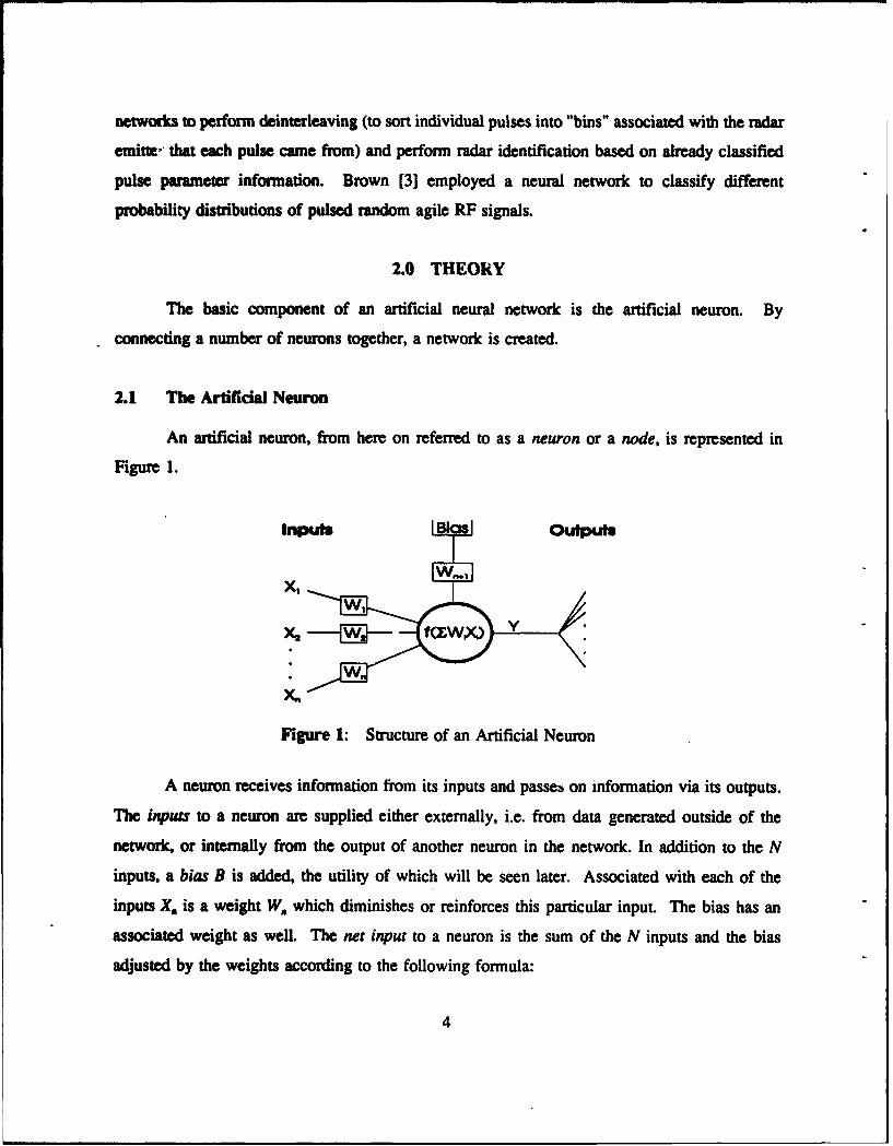
An artificial neuron, from here on referred to as a neuron or a node, is represented in

Figure 1.

xn.

Figure 1: Structure of an Artificial Neuron

A neuron receives information from its inputs and passeb on information via its outputs.

The inputs to a neuron are supplied either externally, i.e. from data generated outside of the

network, or internally from the output of another neuron in the network. In addition to the N

inputs, a bias B is added, the utility of which will be seen later. Associated with each of the

inputs X. is a weight W. which diminishes or reinforces this particular input. The bias has an

associated weight as well. The net input to a neuron is the sum of the N inputs and the bias

adjusted by the weights according to the following formula:

4

To produce the final output y, the net input is further process,-d by a (usually) non-linear

transformadon, called a transfer funcdon or actvation function. The most common transfer

functions (step, ramp, and signoid) are represented in Figure 2.

S0 if x< -a0 Ifx<O 1 if x>a 1Y" {ioeizerwise Y=Y

1a+ I2 otherwise 1+e-ax- -~ 2

0 0 0

a) step b) ramp c) sigmold

Figure 2: Common Transfer Functions

A displacement of these functions along the x axis can be obtained with the bias

(generally set to 1) multiplied by its weight - a positive weight res *l:ing in a displacement of

the function to the right, a negative weight resulting in a displacement of the function to the left.

These three functions can also be defined to be symmetric with respect to the x axis with the

function taking on values between -1 and 1 in the case of the step and the ramp, and between

-4 and ½ in the case of the sigmoid.

Note that any function defined over the input domain, that is monotonically increasing,

has a lower and upper limit, can be used as a transfer function. With its binary output, the step

is the simplest of these functions. Finally, some networks modify the behaviour of a node by

5

generating different outputs based on whether the value generated by the transfer function

exceeds a threshold.

While these transfer functions are the most common, they are not necessarily adequate

for all applications. Some applications use a training algorithm that relies on the differentiability

of the transfer function. The step and the ramp functions, being non-differentiable at the points

of transition, are used in less sophisticated training algorithms.

2.2 Neural Network Types

In the previous section, structure of the neuron was described. This section deals with

the physical organization of the neurons, and the pattern of connectiors that exists between them.

The neurons are usually organized in layers. The number of layers in a network varies

from a single layer to multiple layers. In networks containing three or more layers, the middle

layers are called hidden layers as they have no direct connection to the outside of the network.

The first layer of the network, called the input layer, receives data simultaneously at each of its

nodes, hence the notion of an input vector. At the output layer of the network, the outputs are

generated in parallel to yield an output vector.

The nodes of a network can be connected in different patterns (see Figure 3):

Feed-forward: The flow of information is transmitted from layer to layer from

the input layer to the output layer, with no feedback between layers or

nodes. There are no connections between nodes occurring in the same

layer, so no information is exchanged between nodes in any given layer.

Lateral: Every node is connected to every other node in the network. Recursive

connections are permitted as well (a node can be connected to itself).

Since there are no layers per se, networks of this type are often referred

to as mono-layered networks.

Feedforward/Feedbackward: During the learning or training phase, information

is transmitted from one layer to the next in both directions (from the input

layer to the output layer and vice-versa). The number of weights is

therefore double that of feed-forward networks.

6

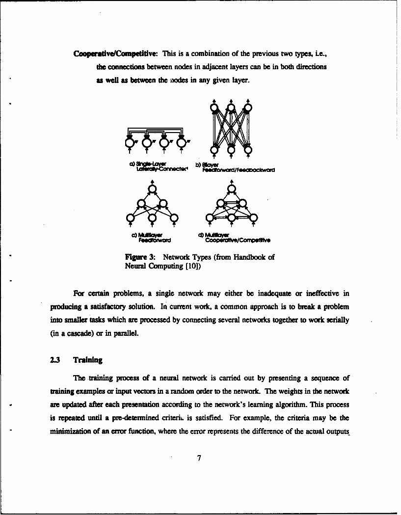
Cooperadve/Compeiltlve: This is a combination of the previous two types, Le.,

the connections between nodes in adjacent layers can be in both directions

as well as between the nodes in any given layer.

bI

Fgeda d Caop flv/Compffiewe

Figre 3: Network Types (from Handbook ofNeural Computing [10])

For certain problems, a single network may either be inadequate or ineffective in

producing a satisfactory solution. In current work, a common approach is to break a problem

into smaller tasks which are processed by connecting several networks together to work serially

(in a cascade) or in parallel.

2.3 Training

The training process of a neural network is carried out by presenting a sequence of

training examples or input vectors in a random order to the network. The weights in the network

are updated after each presentation according to the network's learning algorithm. This process

is repeated until a pre-determined criteri. is satisfied. For example, the criteria may be the

minimization of an error function, where the error represents the difference of the actual outputs.

7

and the expected outputs. The goal upon finishing the training period is to have the network

produce die aticipated result for any input not contained in the set of training vectors. In the

case of sWervi•ed traini•g, a pair of vectors is presented to the network: an input vector and

a corresponding output vector. When the network is presented with an input vector, the

generated output should match the corresponding output vector. If the input and output trai

vectors are the same, the training process is said to be auto-associative, otherwise it is said •

betero-associative. There is also an intermediate form of training called reinforcement in which

the network is simply informed if the output is correct or not. In the case of unsupervised

training, only the input vector is supplied.

In contrast to other systems, a characteristic attribute of neural networks is their ability

to store information in the form of weights on the connections. Before training, the values of

the weights are random, but as training proceeds, the network stores the information by changing

the values of its weights. This information is distributed throughout the set of nodes. The

weights therefore represent the network's current state of knowledge. Each individual training

vector influences the entire set of weights and each individual weight depends on the entire set

of training vectors.

2.3.1 Training Algorithms

A training algorithm specifies the way in which weights in the network are to be updated

in order to improve the network's performance. In the case of supervised training, the algorithm

is usually a variation of one of the following three types [7]:

Hebbian learning: The weight of an input connection to a node is increased if

the value associated with the input connection and the value of the node's

output are both large. This algorithm is designed to simulate the

phenomena of learning through repetition and the formation of habits.

Delta rule learning: The input connection weights of a neuron are adjusted so

as to reduce the error between the actual output and the desired output of

the neuron.

Competitive learning: The nodes in a layer compete amongst themselves. The

8

node that generates the greatest output for a given input modifies its

weights to generate an even greater output. The other nodes in the layer

modify their weights to decrease their output.

Unsupervised learning is less commonly used. The basic idea is that the network

organises itself so that each output node responds (generates a large output) to a set of input

vectors possessing a paricular characteristic.

2.4 Summa

In this chapter, the micro-structure, the macro-structure and the training algorithms of

artificial neural networks have been described. In a continuous attempt to improve the

performance of neural networks, researchers have developed a wide variety of networks: the

Perceptron, the Madaline, the Adaline, Brain-State-in-a-Box, Hopfield nets, back-propagation

networks, self organizing networks, Boltzman machines, and networks that apply adaptive

resonance theory, to name but a few. Among this vast choice of networks, back-propagation

networks are without doubt the most popular and the most commonly used. This is due to the

simplicity of their training algorithms and their effectiveness in handling an ever growing number

of practical applications. Training with feedback (back-propagation) will be the subject of

discussion in the following chapter.

3.0 BACK-PROPAGATION

3.1 Background

Back-propagation (or feedback) training is used in networks containing multiple layers:

an input layer, an output layer, and one or two hidden layers. More than two hidden layers could

be used if desired, but it has been proven that no advantage is to be gained in doing so [10]. The

nodes in the input layer have a linear transfer function which distributes the input values to all

of the nodes in the next layer. For all subsequent layers, including the output layer, the transfer

functions of the nodes are non-linear and generally sigmoidal in nature. (As will be seen later,

back-propagation learning relies on the uniform differentiability of the transfer function. The

sigmoid function satisfies this constraint.) The connections are strictly feed-forward and the

9

UMaing is supervised.

The aim of the back-propagation learning rule (often referred to as the Generalized Delta

Rule), is to minimize the difference between the actual output and the desired output, of a

network for the entire set of input training vectors. To accomplish this, training vectors are

presented one by one to the network, and for each one, the error is minimized by adjusting all

of the weights in the network. In effect, all of the nodes, ncluding their input weights, are

jointly responsible for the global error. The adjustment is based on the gradient method (a

method commonly used in optimization problems). This method consists of stepping along the

error function to be minimized in the opposite direction of the gradient, i.e., in the direction

where the value of the function decreases. For non-linear problems, as is the case here, the

method must be used iteratively until convergence is attained. The number of iterations, or

presentations necessary before convergence to a minimum point is obtained is extremely variable,

being typically anywhere between 100 to 10000. The training period required using the

back-propagation technique is in general a lengthy one, which is the principle weakness of the

technique. Another problem inherent in this algorithm, is that there is no guaranty that the

minimum value found is indeed the global minimum, and in fact is often just a local minimum.

Furthermore, there is no guaranty that the global minimum of the error function is actually zero.

It is incumbent upon the user, therefore, to verify that the minimum found is satisfactory for his

particular application.

Once the training process is terminated, the performance of the network is evaluated with

a set of test cases. This set of test vectors must be completely disjoint from the set of training

vectors, as the network may provide excellent results for the training vectors but yield mediocre

results for other vectors. This would indicate that the network has only learned specific cases,

rather than acquiring the ability to generalize (interpolation for new input vectors becomes

impossible). This phenomena can arise if the network is over-trained.

3.2 Output Layer Learning Rule

The goal of back-propagation learning is to adjust the weights in the network so as to

minimize the error function. This is done by comparing the output vector with the desired output

10

vector and adjusting the weights, starting with the output nodes and working backwards to the

input nodes. In a network with N inputs and L hidden nodes arranged in a single layer and M

outputs, the erro to be minimized for each training vector is the stun of the squares of the

outumm. Therefore, the global error for a training vector p is given by:

I 2

whoem a is the error for the vector p at the output node k between the expected output value y,•

and the actual output value oj.

To determine the relative responsibility and the direction in which each weight will be

adjusted, the gradient of the error VE, with respect to the weights wk (weights associated with

the connection between node j and node k) is calculated. Each weight in the output layer is

adjusted proponiomally in the negative direction of the partial derivative of the error E, with

respect to this weight

= @

(=yp - o0 /• (nett)j, (3)

where ae• is the net input, f' the derivative of the transfer function, Ok the bias of the output

node k and im the output of the node j in the hidden layer. Note that because the partial

derivatives make use of the derivative of the transfer function, this function must be differentiable

for all values. The new weight is obtained by adding an amount proportional to the partial

derivative to the former weight. With a constant of proportionality'T, the adjusted weight is

obtained by using the following formula (see [4] for the complete derivation):

*t+ 1) = 4() + - o,,-of•'(netiJLW (4)

11

(A I •wo + P8J(nt Wi, 5

Fiully, by deMining a value 68 - 6W,'Q (noo, one obtains

4 +l + ()18ýi'W (6)

3.3 HldM= Layer LMarhuhg Rule

As dh error also depends on the weights associated with the hidden layers of the network,

similar calculams to thoe done for the weights associated with the output layer must be done

for these weights as welL The error E for the hidden layer can be expressed as a function of

the outputs of the bidden layer:

N L-Ir yk -kl(r + D)2(7)

Using this equation to calculate the gradient with respect to the weights w" in the hidden

layer, the following equation is obtained:

h

If an adjustment, proportional to the partial derivatives with a constant of proportionality

equal to 11 is made, then the value of dte adjusted weight is given by (see [4] for the complete

derivaion):

G4Xt +1) + VJA(nedW V (Y - ok (4o90'); (9)

S M

* ~)+ eJ(ndet)XP 8a01 (10)k-I

Notice thatthe new 8 depends on all of the 8ý of the output layer. In the case of a

12

network containing more than one hidden layer, the equation would be similar, except that the

new 8 would depend on the 6, of the second hidden layer instead of the output layer. This is

why the adjustment of the weights begins at the output layer, tier, continues from layer to layer

in the opposite direction from the usual flow of information (hence the term back-propagation).

3.4 Internal Behaviour

In the process of iterative training, the nodes in the hidden layers detect different

characteistics found in the input vector in the sense that their outputs are activated (output value

is large) if they detect a particular characteristic and are deactivated (output value is small)

otherwise. Since there are usually fewer hidden nodes than input nodes, this phase of training

is comparable to a reduction in the number of dimensions of the input space. If the network is

used for the purposes of classification, the nodes in the output layer arrange themselves to

partition the output space into separate regions based on the characteristics supplied by the hidden

nodes. In general, each separate region represents a distinct class of the inputs.

When training is finished, the test vectors are presented to the network. The network

interprets these new vectors by detecting the absence or presence of characteristics already seen

in the training vectors. If a good generalization has been obtained, and a test vector shares

common characteristics with a class of training vectors, then the network provides excellent

results. The network can respond to new test vectors by interpolating a response from the set

of training vectors. For example, if the network generates an output A' from a training vector

A and an output C' from a training vector C, then, if B is "between" A and B, the network will

generate B' between A' and C". The network does not in general provide good results in the

context of extrapolation. The network does not learn features when it has never been given

examples containing these features. Note that an addition of noise is considered to be an

interpolation and not an extrapolation as the prime characteristics are still present and the noise,

only adds superfluous information that is removed by the network.

13

3J Variatious of Back-propagation Training

One of the principal drawbacks of the back-propagation technique is its slow training

time. One of the ways to accelerate the learning time is to use a large learning coefficient (the

value q in equation 6 in section 2.2 and in equation 11 in section 2.3). A large learning

coefficient in theory, permits faster training times, since the steps taken in the opposite direction

of the gradient are greater. This has the potential drawback, however, of causing oscillation of

the total error when the curvature of the error surface is great. As the algorithm assumes that

the surface is locally linear, the steps taken will continuously overstep the global minimum. A

small learning coefficient stabilizes this process, but results in very long training periods. In

addition, it increases the likelihood that the algorithm will become trapped in a local minimum.

To alleviate these problems, variations of the original algorithm have been developed.

3.5.1 Varying the Coefficients

One can accelerate the training process by varying the value of the learning coefficient

By starting with a large value for T1, large steps can be taken to quickly move towards the

minimum of the error function and to avoid being trapped in a local minima. As training

progresses, the value of iq can be lowered to prevent oscillations about the global minimum.

3.5.2 The Momentum Method

A common method to speed up learning is the momentum method. As its name indicates,

the momentum method consists of adding momentum in the direction of the weight change. In

calculating a new adjustment to the weights, it takes into account the previous adjustment

Therefore a fraction o: of the previous step is added to the formula to produce the following

equation:

(0(t+1) = ()+ q8•i, + aV,4(t-1) (12)

whenr a is between 0 and 1. The new term acts as a low-pass filter on the weight error and

reduces the oscillation of the network's global error, because it favours a continuation of

14

movements in the same direction. With this method, faster rates of learning are obtained, while

keeping the learning coefficient il small at the same time.

3.5.3 Cumialtive Update of Weights

Cumulative back-propagation is another method that can improve the rate of convergence

of the algorithm. It consists of accumulating the error for several pairs of input/output training

vectors before updating the weights. When a single update is made, the error function is reduced

for that particular pair only. The overall error function may actually increase. A global update,

on the other hand, guarantees a reduction in the overall error function. Caution must be

exercised though; the number of calculations greatly increases with the number of accumulated

training pairs. The benefits of this technique are lost if the number of pairs is too large.

3.6 Summary

This chapter has described the back-propagation learning rule, its internal behaviour, and

three methods for accelerating the training process. The next chapter covers a number of

practical considerations, that all neural networks builders must deal with when constructing

networks to effectively solve concrete problems.

4.0 PRACTICAL CONSIDERATIONS

Two important practical concerns in the design of a network are:

Convergence of the error function: A problem that can occur during the

training period that will prevent convergence is node saturation. For

transfer functions such as the sigmoid that attain their minimum and

maximum values asymptotically, a large input at a node will be mapped

into a region of the sigmoid whose derivative is virtually zero. If the

derivative is zero, the learning adjustment will be zero, which implies that

the node ceases to learn. When this happens, the node is said to be

saturated. If too many nodes become saturated during training, learning

could simply stop before a minimum in the error function can be found.

15

The speed of convergence is also an important consideration. Some

techniques for accelerating the training period for back-propagation were

described in tie previous chapter.

Network perlftrmamn: It is important that the network perform efficiently and

effectively on real inputs when the training period is finished.

There are a variety of techniques that address these network design issues. These am

described in the following sections.

4.1 Pre-treatment of Input Data

Raw data is rarely presented to a network without some form of pre-treatment. In certain

cases, to ensure convergence of the error function, a simple normalization of the input and output

vectors is performed to map the data values to within a narrow zone (outside of the asymptotic

regions of the transfer function). For example, input values should be normalized to lie within

the range [-1, 1] and the output training values to lie within [0, 1]. Freeman and Skapura [4]

suggest an additional precaution when the transfer function of the output nodes is sigmoidal:

normalize the output training values to [0.1, 0.91 rather than [0.0, 1.0] to avoid saturation of the

nodes, since the values of 0.0 and 1.0 can only be obtained asymptotically at the output of this

transfer function.

In other cases, the pre-treatment of the input data requires more attention. A

transformation may be necessary to eliminate insignificant variations and ruperfluous details

(translations, rotations, deformities, ...) while at the same time accentuating the pertinent

information. Without doubt, the most commonly used transformation is the Fourier transform,

but other transformations such as the Cepstrum, the Gabor transform and the spectrogram are

used as well. Recently, Principal Component Analysis (PCA) has received attention [101. This

technique reduces the number of dimensions of a problem, but keeps the parameters for which

the eigen vectors of the autocorrelation matrix have the greatest energy. When the dynamic

range of a variable goes beyond several octaves, a logarithmic transformation may be necessary

to retain the small variations that might otherwise be lost in normalization. There are other

techniques such as Feature Extraction in which only the important characteristics of the raw data

16

are presented to the network as inputs. This reduces the work and complexity of the network but

one must ensure the relevance of the chosen characteristics. In general, it is difficult to know

in advance which transformations will produce the best results. Experimentation is often required

to determine the best approach.

If the network is to operate in a noisy environment, then once the inputs have been

transformed and normalized to fit the application, appropriate noise must be added to any

synthetically generated training vectors. Freeman and Skapura [4] have found that noise added

to the inputs can facilitate the convergence of the network even if the network is destined to

operate in a clean environment.

4.2 Weight Initialization and Adjustment

Before training begins, the weights in the network are n.ndomly initialized. It is

recommended that values of the weights lie between ±0.5 (some authors recommend even lower

limits). Doing so prevents the neurons from saturating at the outset of training. Once training

is in progress, it is important that the training vectors be presented in a random order so that the

network learns the characteristics of the inputs rather than a specific order of inputs. Of even

greater importance is to avoid presenting all of the vectors of one class, followed by the vectors

of the second, and so on. There is a risk that the network will forget what it has learned from

the preceding class during the training of the next class.

Another method of preventing saturation in the nodes is to add a small quantity e to the

derivative of the transfer function. As the adjustment of the weights depends on the derivative,

this e permits a slight adjustment to nodes that would otherwise cease to learn.

4.3 Choosing the Number of Training Vectors

Choosing the correct number of training vectors is an important consideration. When

there are not enough vectors in the training set, there is a risk that the network will fail to

generalize. The network will produce correct results for vectors in the training set but will fail

on test vectors. According to the Baum and Haussler result [6], if the allowable error for any

test vector is to be less than e then the network will "almost certainly" generalize if the allowable

17

error for the training vectors is less than 0 and the number of training vectors is greater than

W/e where W equals the number of weights in the network. For example, if the test vectors are

to have erros less than 0.2 and there are 200 connections in the network, then there should be

at least 1000 training vectors and the training should proceed until the value of the error function

is less than 0.1.

4.4 Network Design

The decision concerning the number of layers and nodes to use for a particular application

is of great importance as it influences the likelihood that the error function converges and that

the network generalizes. While there are heuristics to guide these choices, experimentation is

often required to achieve acceptable results. This experimental aspect is one of the prime sources

of criticism directed towards the neural network approach.

4.4.1 Number of Layers

Because the computational performance of the network is directly proportional to the

number of layers and nodes, it is desirable to limit these values as mucl as possible. It has been

proposed that in most cases one or two hidden layers is sufficient. The neural network

interpretation of Kolmogorov's theorem by Hecht-Nielsen proves that a network with a single

hidden layer, whose nodes have transfer functions that are not constrained to be the same, can

represent an arbitrary function of the inputs [10]. Unfortunately, the theorem does not say how

to choose the transfer. functions and has therefore little practical application. Cybenko shows that

two hidden layers, whose nodes all use sigmoidal transfer functions, are sufficient to compute

an arbitrary function of the inputs, and that a single hidden layer is sufficient for classification

problems [10]. According to Maren et al. [10] experimentation has confirmed these results.

4.4.2 Number of Modes Per Layer

The number of nodes in the input layer is fixed by the number of points in the input

vector. For the output layer, the number of nodes is set to the number of desired outputs (e.g.

classes, categories, probabilities). Any attempt to reduce the number of nodes in the output layer

18

by an encoding of the outputs should be applied with caution, as the additional burden imposed

on the network may only prove workable with the inclusion of a second hidden layer.

Choosing the number of nodes in the hidden layers is more difficult. The objective is to

keep the number of nodes to a minimum as the addition of extra nodes can result in a network

that learns particular cases, yet fails to learn general characteristics, as well as increasing the

training and operational complexity. Here again, the decision can be guided by theoretical and

empirical limits. According to Hecht-Nielson's interpretation of the Kolmogorov theorem, 2N

+ 1 nodes (where N is the number of inputs) are necessary to calcul,,te an arbitrary function.

According to Kudrycki, the optimum ratio between the first and the second hidden layer is three

to one [10]. For small networks where the number of inputs is greater than the number of

outputs, it has been proposed that the geometric average of the inputs and outputs provides a

good estimate of the optimum number of nodes to use. There is general agreement however, that

the number of nodes in each hidden layer should be fewer than the number of inputs.

4.5 Summary

This chapter has dealt with practical considerations in the design of a network. The ta

main issues are convergence of the error function and network performance. A number of

techniques that address these issues were presented, including pre-treatment of the input data,

weight initialization and adjustment, the number of vectors in the trining set, and the choice of

the number of layers and nodes in the network.

5.0 CLASSIFICATION OF RADAR SIGNALS

The advent of complex radar systems has lead to the appearance of frequency and pulse

repetition interval (PRI) agile emitters. Emitters can vary these parameters, either randomly or

periodically following a well defined modulation pattern. The application of neural networks

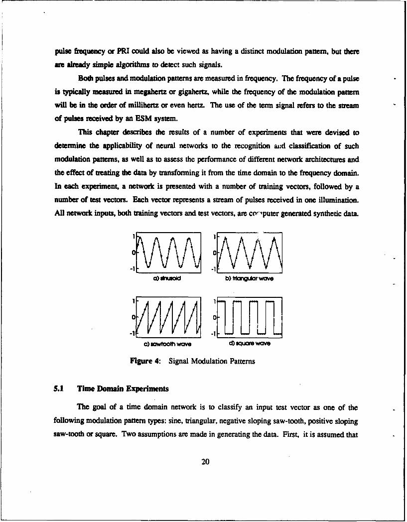
described in this paper is limited to the common modulation patterns shown in Figure 4. (The

vertical and horizontal axes represent the frequency of the pulse and the time of arrival

respectively). These include the sinusoid, the triangular wave, the sawtooth wave (including both

negative and positive sloping teeth) and the rectangular wave. A signal exhibiting a constant

19

pulse frequency or PRI could also be viewed as having a distinct modulation pattern, but there

are already simple algorithms to detect such signals.

Both pulses and modulation patterns are measured in frequency. The frequency of a pulse

is typically measured in megahertz or gigahertz, while the frequency of the modulation pattern

will be in the order of millihertz or even hertz. The use of the term signal refers to the stream

of pulses received by an ESM system.

This chapter describes the results of a number of experiments that were devised to

determine the applicability of neural networks to the recognition ad classification of such

modulation patterns, as well as to assess the performance of different network architectures and

the effect of treating the data by transforming it from the time domain to the frequency domain.

In each experiment, a network is presented with a number of training vectors, followed by a

number of test vectors. Each vector represents a stream of pulses received in one illumination.

All network inputs, both training vectors and test vectors, are cvriputer generated synthetic data.

a) *iwold b) ftkngulr wove

-1 1

0-0

C) swtoolh wave CO square wave

Figure 4: Signal Modulation Patterns

5.1 Time Domain Experiments

The goal of a time domain network is to classify an input test vector as one of the

following modulation pattern types: sine, triangular, negative sloping saw-tooth, positive sloping

saw-tooth or square. Two assumptions are made in generating the data. First, it is assumed that

20

all radar pulses seen in an illumination are equidistant in time, i.e. constant PRI, and second, it

is assumed that the signal average is zero, i.e. no DC component is added to the signal generation

equations. (For real data, a pre-treatment step to subtract the average value, assuming it is

non-wro, is necessary.) It is also assumed that the parameters vary as follows:

Time: The length in time of an illumination is variable. In other words, an

illumination may contain a variable number of pulses.

Frequency: The frequency of the modulation pattern can also be viewed as a

variation in the number of periods contained in one illumination. The

number is assumed to be relatively small, varying between one period and

three periods.

Phase: An illumination can start at any point in the cycle of the modulation

pattern; the phase shift varying anywhere between 0 E=d 2z.

The classifier must find shared characteristics in the inputs, subject to the above parameter

variations, that permit it to differentiate between different signal patterns.

All of the networks used in the experiments are of the back-propagation type, all have a

single hidden layer, and all use the cumulative update training method. The elements of an input

vector represent the pulse frequencies in a single illumination. The output vector contains one

element for each possible modulation pattern. The element with the highest value is taken to be

the classification of the input signal.

Two sets of experiments were carried out. In the first, the number of pulses per

illumination is assumed to be no more than 16, and in the second, no more than 32. Where the

illumination contains fewer pulses than the maximum, the corresponding vector is padded with

zeoes.

Before generating training and test vectors, the number of nodes in the various layers must

be decided upon. According to the Baum and Haussler result, in order to obtain an error of less

than e in the test vectors, the number of training vectors must be at least l/e times the number

of connections in the network. For these experiments e was chosen to be 0.2. Therefore the

number of training vectors must be at least five times the number of connections in the network.

To compare the relative merits both in terms of performance and training times, five different

networks were built for each set of experiments. In the first network, the number of nodes in

21

the hidden layer was equal to the number of nodes in the output layer, in the second network,

the number of nodes in the hidden layer was equal to two times the number of nodes in the

output layer, and so on. This was done to test the Kudrycki hypothesis that the ratio of the

number of nodes in the hidden layer to the output layer should be three to one.

The notation used in this paper to define the architecture of the various networks is i-h-o

where i indicates the number of nodes in the input layer, h the number of nodes in the hidden

layer, and o the number of nodes in the output layer. The networks used in the first set of

experiments are therefore denoted as 16-5-5, 16-10-5, 16-15-5, 16-20-5, and 16-25-5.

The number of weights or connections in a three layer back-propagation network is given

by (i * h) + (h * o). For the above networks this yields 105, 210, 315, 420, and 525 connections

respectively. Using the Baum-Haussler rule, the number of training vectors to be generated for

each network should be at least 525, 1050, 1575, 2100 and 2626 respectively.

In generating the training vectors, there are four parameters of concern: the number of

different classifications (or output nodes), the variation in the number of pulses in the

illumination (in this casz, some number between 1 and 16), the variation in the number of period.

in the illumination and the variation in the pha.,e. The basic algorithm for generating the training

vectors is as follows:

FOR EACH classification type c DOFOR x = pulse min TO pulse max BY pulse step DO

FOR y = period min TO period max BY period step DOFOR z = phase min TO phase max BY phase step DO

Gernerate a new vector v (c, x, Y, z);Generate the corresponding output vector w;Output v and w;

ENDEND

ENDEND

To avoid saturation, the entries in the input training and test vectors are computed so as

to lie within the range of-I to +1, and as Freeman [4] suggests, the entries in the output training

vector all lie within the range of 0.1 to 0.9.

To give equal weight to each of the variations, the number of possible values taken on

by each of x, y and z in the above algorithm should be the same, say n. The number of training

22

vectors geneid is then equal to Cn3 , where C is the number of classifications, i.e. the number

of output nodes. To satisfy the Baum-Haussler result n must be such that Cr? is greater than or

equal to five times the number of connections in the network. The value of n can therefore be

computed by taking the ceiling of the cube root of 5/C times the number of connections in the

networ. Since C is %ual to five in this case, n is simply equal to the ceiling of the cube root

of the number of connections in the network. Table I shows the minimum number of training

vectors to be generated to satisfy Baum-Haussler, and the actual number of training vectors that

were generated for all of the time domain network experiments.

The parameters x, y, and z are evenly spread across the desired range of values. For

example, if the period of the modulation pattern is to vary between one and three, and five values

are to be computed, then the values will be 1.0, 1.5, 2.0, 2.5 and 3.0. If seven values are needed,

the values could be 1.002, 1.335, 1.668, 2.001, 2.334, 2.667, and 3.0. Table U shows the number

of values desired for each variation (n), and the minimum, maximum and step size required to

compute values for x, y, and z. The first five rows show the range of values used to generate the

training vectors for the 16 input networks. The sixth row shows the ranges used to generate the

test vectors used in testing all of the 16 input networks. The ranges used to generate the training

and test vectors for the 32 input networks are shown in the subsequent six rows.

The test vectors are generated using the same algorithm, although care is taken that no

test vector is identical to any of the training vectors. This is to ensure that the network is tested

against previously unseen vectors.

The second set of experiments was carried out using networks with 32 entries, i.e, 32-5-5,

32-10-5, 32-15-5, 32-20-5, and 32-25-5. Apart from the change in dimension of the input vector,

the same algorithm was used to generate the training and test vectors.

The actual experimental process consisted of generating the training and test vectors, and

building the corresponding network using the commercial product NeuralWorks Professional II,

produced by NeuralWare Inc. Each network was initially presented with 20,000 training vectors

randomly chosen from the generated training vector set. (The number 20,000 was determined

experimentally to be a convenient interval for assessing the improvement in performance over

time.) The performance of the network was then determined by computing the percentage of

23

cXrecy classified signals represented by the test vectors. Every network used in these

expeiments has five outputs, each output corresponding to a particular classification. A signal

is considered to be correctly classified if the value in its associated output node is greater than

any value in the other output nodes. Although this is a weak measure of success, it is sufficient

for comparison purposs. (A stronger measure of correctness would insist that not only should

the associated output node's value be the greatest, but that it exceed some threshold as well.)

In addition to the performance of the network, the length of time required to train the network

with the 20,000 vectors is recorded. The training and testing process is repeated for a total of

20 times (400,000 presentations of training vectors). Table III shows the results for the networks

with 16 inputs, and Table M, Table IV shows the results for the networks with 32 inputs.

Figure 5 to Figure 14 in Appendix A show the results in a graphical format.

24

Netwoat Number of Required Number of Actual

Connect- Number of Variations Number of

ions Training (n) Training

(Weights) Vectors Vectors

16-5-5 105 525 5 625

16-10-5 210 1050 6 1080

16-15-5 315 1575 7 1715

16-20-5 420 2100 8 2560

16-25-5 525 2625 9 3645

32-5-5 185 925 6 1080

32-10-5 370 1850 8 2560

32-15-5 555 2775 9 3645

32-20-5 740 3700 10 5000

32-25-5 925 4625 10 5000

Table I: Tune Domain: Number of Training Vectors

25

NecL a Pulse Pulse Pulse Period Period I Period Phase Phase Phase

min max step min I max step min max step

16-5-5 5 12.0 16.0 1.0 1.0 3.0 0.5 0.0 1 0.996 0.249

16-10-5 6 11.0 16.0 1.0 1.0 13.0 10.4 00 i0.995 0.199

16-15-5 7 10.0 16.0 1.0 1.002 3.0 i0.333 0.0 0.996 0.166

16-20-5 8 9.0 16.0 1.0 1.005 3.0 10.285 0.0 10.994 10.142

16-25-5 9 8.0 16.0 1.0 1.0 13.0 10.25 0.0 10O.99 0.124

Tes 16 4 9.0 15.0 12.0 1.001 12.999 10.666 0.0 , 0.999 I°0.333

32-5-5 6 27.0 32.0 11.0 1.0 .3.0 0.4 0.0 0.995 0.199a I I-1-41 1~32-10-5 8 25.0 32.0 1.0 1.005 3.0 10.285 0.0 i 0.994 0.142

32-15-5 9 24.0 32.0 1.0 1.0 1 3.0 1 0.25 0.0 1 o.9 10.124

32-20-5 10 23.0 32.0 1.0 1.002 3.0 10.222 0.0 !0.999 i0.111- - i a -

32-25-5 10 23.0 32.0 1.0 1.002 1 3.0 10.222 0.0 .0.999 j0.111Test 32 4 25.0 1,31.0 2.0 1.001 12.999 0.666 0.0 10.999 10.333

- |i - - ml -: 1

Table Rh Tume Domain: Pulse Count, Period and Phase Settings

26

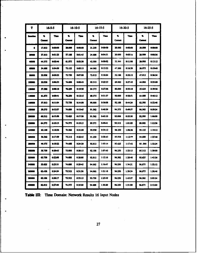
T 16-5-5 16-10-5 16-15-5 16-20-5 16-25-5

- M- W C- c - -com-

0 17.312 0:00"0 0W 0:00:00 21.2.50 n 04M 20000 0:00:00 20.000 0:0M

201W 37.812 0*0:2M 37.1a 1 0:014 31 0:"04..31 20.000 0:0.-. 20.000 0:M6

46M 44315 0OM46 W1.375 0:03:30 42.500 000* 32.500 0:11:06 2.0A0 0:13:12

4 AmW 5441. 0:" 712 0:0:515 64.062 0:13:33 47.00 0:.16:3 26.875 0.19:43

-am-1 55.9S8 0:0032 71750 0:07:00 72.812 0:!8:4 52.113 0:.2212 47.812 0:"

1to=3 55.933 0:06:55 74.A3 0:0D45 85.312 0-2235 69.062 0.27A5 4,.04 0:.33:0

120 57.5W 0:0M:18 74.M0 0:10:30 4.375 0:27.I06 0.000 0:33:13 "M.425 0:.39:2

14HOW 61.85 0:0471 76,250 0:12:15 39.37 &337 90W000 0W33:51 64.60 0.46:12

1411 5•.11 0:1104 713.70 0:14:00 0.000 0:36:0M 92.18 0:.4:24 82.500 0-.524

11110 57 0:12:27 74.63 0:15:5 91.562 0:40:M9 949375 O:.4957 W 0:

210W .312 0:13M4 75.•5 0:17M4 91.543 0:45:10 95.000 0:55:30 92.500 1.:0"

"2211W 44375 0:15:.13 74.375 0:19:15 19.375 0:49:41 95.312 1:01:03 39.02 1:12M36

am0W = .118 0:16:36 74.082 0:21:00 90.938 0".54:12 96.250 1.06:36 93.125 1:19:12

0 000 362 0:17:* 75.312 0:2245 91.250 0:58:43 95.938 1:12:3o 94.613 1:25.48

3&00M 5 0:19:22 74.488 0.-2:30 92.812 1.:03:14 95.625 1:17A42 95.000 1:32:24

W 58.73A 0:20:45 75.000 0.26:15 92.13 1.07:45 96.250 1:23:15 95.312 1:39:00

6173 0:220 74463 0:200 92.812 1:12.16 96.562 1:283:4 95.625 1:45:36

340000 55 0:23:31 74A08 0:2.9:45 94.062 1:16:47 96&250 1:34:21 96.375 1:52:12

3 1 643 = :2454 71.312 0:31M4 9C4.04 1.21:18 96.250 1:39-54 96.75 1A58M

WUO0 6.13 0:26:17 751312 0:.33:15 93.750 1:25A49 96.250 1:45:27 9L6.52 205:24

4M0600 3 0:27U40 74.375 0".35: 94613 1:30:20 96.250 1:51.00 96.75 2.12:00

Table 1l: Time Domain: Network Results 16 Input Nodes

27

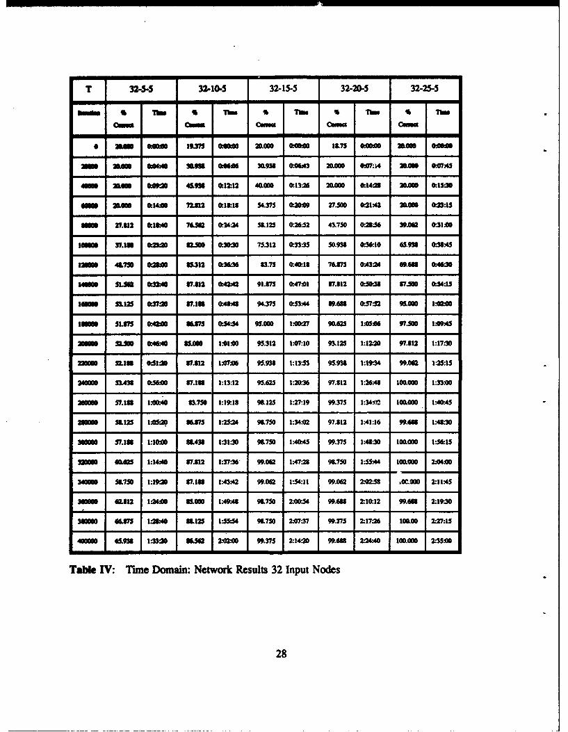
T 32-5-5 32-10-5 32-15-5 32-20-5 32-25-5

Sol" T"m TIM Sb Ti S Tim•mm8 C•mt CON" (scn c•m"

0 am 00m 19.375 A:00.0m 20.000 0:0000 18.75 @O.:0: 31.m0 0Om0

Um3 0 28A00 :4S 50.93 0.06.06 20.933 0:06A3 20.000 0.07:14 25,000 0:745

4m300 Am.3 0G0o30 45.93 0:12:12 40.000 0W13-26 20.000 0:14M0 X0.000 0:15:30

4 U 30.0 0:14M0 72.312 0:!1:13 54.375 0t20409 27.500 0:21A2 3.00 0621:15

I0I 2V.312 0:18A40 76- 0,34:24 5L.125 0.26U52 43.750 0.21.56 39.031 0.31:00

100l00 37.18 0:" Woe 0:30:30 75.312 0:.33".35 50.91 0-.6:10 65&9W 0:36.45

123300 43.L70 0:2310 3I312 03L3W 83.75 040.18 76375 00.43:2 M9A.N 0:46k30

14H300 51.$3 0:1140 17.812 0.42:42 91.375 0:.47:01 W7.812 00.50"J8 V7.500 0.54:15

I 51125 0:3720 1.l 0:4W-.43 94.375 00M$4 39.401 0:.57:52 91.000 1:02

133300 51.375 0S42m0 16.7L5 0:54:54 95.000 1.100.27 90.625 105:06 97.500 110W45

20300 52.30 0e 85.0 1O01i00 95.312 I.07:10 93.125 1:12:20 97.812 1:17:30

25000 ,52,1N 0:5120 81.812 1.0706 95.938 1:13.53 95.933 1:19:34 99.062 125:15

240000 53.438 0.56.'00 7.101 1:13:12 95.625 1:20.36 97.812 1:26.43 100.000 1:33.00

2500)0 7.13 1:000 85750 1:19:13 90.125 1:27:19 99.375 1:34'2 10.00o 1:40.45

30000 5.125 10:20 36.375 1-2524 9L.750 1:34:02 97.812 1.41:16 99.4" 1:48:30

30000 37.188 1:10:00 33.438 1.31:30 90.750 1:40.45 99.375 1:48:30 100.000 1:56.15

320000 G0&W 1:1440 V.1112 1.37:36 99.062 1:47:28 90750 1:55:44 100.000 2-4:00

340000 .5.750 1:19"20 10.111 1:43A42 99.062 1:54:11 99.062 2.'258 OriW.0 2:13:45

360000 31.312 l:2:00 5.m0 1.49M43 90750 7.0054 99.633 2:10.12 99.433 2:19-30

330000 3.75 128..40 33.125 1:55:54 90.750 '07:37 99.375 2:17:M 1O0.00 2:27:15

4a0000 m 5.33 1:33:10 305 2.'2.10 "9.375 2:14:M0 99.6M 2:24:40 100.000 2:35:00

Table IV: Time Domain: Network Results 32 Input Nodes

28

5.2 The Frequency Domain

One of the goals of this project is to analyze the performance of neural networks using

data that has been transformed from the time domain to the frequency domain. Transforming

data in this way, most commonly using a Fourier Transform, is a common technique for

analyzing signals in digital signal processing. The Fourier transform is typically applied to an

amplitude versus time representatioa of a signal. This project, however, deals with the

modulation of pulse frequencies over time. A transformation into the frequency domain in this

case yields a pulse frequency versus modulation frequency representation of the signal.

Note that in a fielded application the additional cost of pre-treating data must be weighed

against any possible benefits.

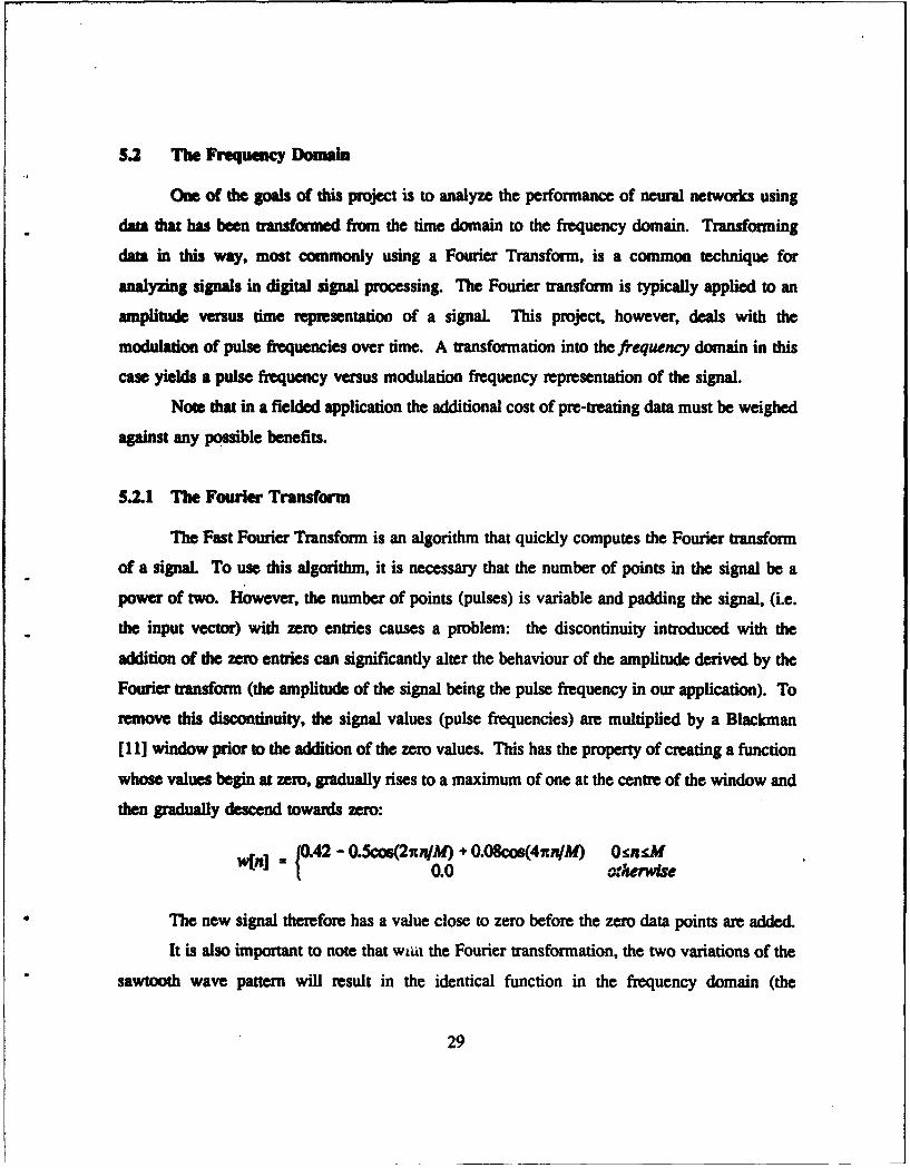
5.2.1 The Fourier Transform

The Fast Fourier Transform is an algorithm that quickly computes the Fourier transform

of a signal To use this algorithm, it is necessary that the number of points in the signal be a

power of two. However, the number of points (pulses) is variable and padding the signal, (i.e.

the input vector) with zero entries causes a problem: the discontinuity introduced with the

addition of the zero entries can significantly alter the behaviour of the amplitude derived by the

Fourier transform (the amplitude of the signal being the pulse frequency in our application). To

remove this discontinuity, the signal values (pulse frequencies) are multiplied by a Blackman

[111 window prior to the addition of the zero values. This has the property of creating a function

whose values begin at zero, gradually rises to a maximum of one at the centre of the window and

then gradually descend towards zero:

win] ={f042 - 0.5cos(2ianIM) + 0"08cos(4xn/M) O=5nsM

SlThe new signal therefore has a value close to zero before the zero data points are added.

It is also important to note that wan the Fourier transformation, the two variations of the

sawtooth wave pattern will result in the identical function in the frequency domain (the

29

transformaion of the negative and positive wave patterns differing by a phase shift of 180

degrees). The total number of distinct signal classifications is therefore reduced to four. The

distinction between the two sawtooth patterns can be easily made after the neural network has

produced its output.

5.2.2 Frequency Domain Experiments

As for the time domain experiments, separate sets of training and test vectors were

generated to serve as input to a new set of neural networks. For these experiments, five networks

with 16 input nodes were created ranging from four hidden nodes to twenty: 16-4-4, 16-8-4, 16-

12-4, 16-16-4, and 16-20-4, and five networks with 32 inputs: 32-4-4, 32-8-4, 32-12-4, 32-16-4,

and 32-204. The basic algorithm to generate the input vectors is the same. Again, the

parameters that can vary are the classification of the signal, the number of pulses in the signal,

the number of periods in the illumination and the phase of the signal:

FOR EACH classification type c DOFOR x = pulse min TO pulse max BY pulse step DO

FOR y = period min TO period max BY period step DOFOR phase min TO phase max BY phase step DO

Generate a new vector v (c, x, y, z);Apply Blackman window to v;Apply Fourier Transform to v;Generate the corresponding output vector w;Output v and w;

ENDEND

ENDEND

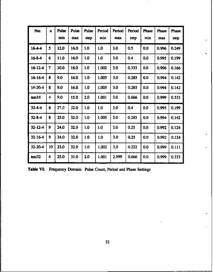
Table V lists the number of training vectors to be generated for each network. Table VI

shows the ranges and step sizes used to specify the x, y and z values of the algorithm. Table VII

shows the results for the networks with 16 inputs, and Table VIII shows the results for the

networks with 32 inputs. Figure 15 to Figure 24 in Appendix A show the results in a graphical

format.

30

Network Number of Required Number of Actual

Connect- Number of Variations Number of

ions Training (n) Training

(Weights) Vectors Vectors

16-4-4 80 400 5 500

16-8-4 160 800 6 864

16-12-4 240 1200 7 1372

16-16-4 320 1600 8 2048

16-20-4 400 2000 8 2048

32-4-4 144 720 6 864

32-8-4 288 1440 8 2048

32-12-4 432 2160 9 2916

32-16-4 576 2880 9 2916

32-20-4 720 3600 10 4000

Table V: Frequency Domain. Number of Training Vectors

31

NtIn Pulse IPulse IPulse Period IPeriod Period Phase Phase IPhase

I minimax I step min I max step min max i step0 1"164-4 ,5 12.0 ;16.0 1.0 1.0 ;3.0 0.5 0.0 0.996 0.249

16-8-4 16 11.0 116.0 1.0 1.0 13.0 0.4 0.0 i0.995 '0.199

16-12-4 17 10.0 16.0 1.0 1.002 ! 3.0 0.333 0.0 10.996 10 166

16-16-4 1 8 9.0 1 16.0 1.0 1.005 1 3.0 10.285 0.0 1 0.994 0.1422! 2 2 . .2

16-20-4 1 8 9.0 116.0 11.0 1.005 13.0 0.285 0.0 10.994 10.142

tt, j4 9.0 .15.0 12.0 1.001 1 3.0 0.666 o.0 i0.999 0•333I

32-44 16 27.0 320 1.0 1.0 1 3.0 0.4 0.0 10.995 0199

32-8-4 1 8 25.0 !32.0 1.0 1.005 !3.0 0.285 0.0 0.994 0.142

32-12-4 19 24.0 32.0 i1.0 1.0 3.0 i0.25 0.0 0.992 0.124

32-16-4 9 24.0 '32.0 1.0 10 30 025 0.0 0992 0124

32-20-4 10 23.0 320 1.0 1.002 3.0 0.222 0.0 0.999 0.1114.i : i - -

test32 14 25.0 131.0 12.0 1.001 12.999 10.666 0.0 0.999 0.333

Table VI: Frequency Domain: Pulse Count, Period and Phase Settings

32

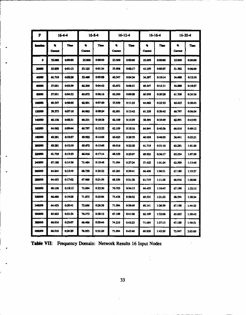
F 16-44 164-4 16-12-4 16-16-4 16-20.43 -•t q Th rsuTrs b Tm Thee I T ime

Camr Cmm cm Caaum t Ckma

O u , O o t& a 2 5 0 0 0 0 0 0 2 5 .0 0 0 0 0 0 :0 0 2 5 .0 0 0 0 .0 0 .0 0 2 5 .0 0 0 0 .0:O 0

20000 si.t 0:01:13 W3.125 0 :01:34 53.06 0.f :17 43.359 00 :07 51 ..5a 00609

40000 61.719 0 2 55.44 0.:020 640.47 0.04:34 54.297 01.10:.14 4.618 0.12.18

60000 57. 631 06 :39 6 0 0:04:42 63.672 0:0f 51 60.547 0.15.2 1 54.61 8 0:18:27

m0000 57.031 0:04:52 G&.672 0:06:16 62.500 0:09:0M 60.938 0.20: . 61.328 0.24:36

100000 60.547 M d6189 1 0.&7:0 55.859 0:.1125 64.062 0:2535 65.625 0.30.45

120000 59.375 0.07:18 64062 000:24 62.391 0:.13:42 61.328 0.30:42 66.797 0:36:54

140000 40.156 0:00:31 69.531 0 O10:56 62.109 0:.15:59 5 8.594 0:35A49 62.891 0:43:03

lo400 64.062 0094 6.797 0.12:32 62.109 0.18:16 64.844 0.40-56 66.016 0.49:12

130000 63.231 0:.10:57 69.922 0:.14.06 65.625 0:.233 60.938 0 .46.03 56.641 0 .55:21

200000 6 ". 81 0: .12:10 63. 67 2 0: .15 0 66.016 0 "22:50 61.719 0:51:10 63.23 1 1:01:30

220000 61.719 0:13:23 M.016 0.17:14 61359 0.25.07 69.922 0:56:17 65.234 1.07:39

240000 67.189 0.14M36 71.484 0 :.13: ' 71.094 0:27:24 57.422 1:01:24 62.500 1:13:48

20000M 64.844 0-15A49 61750 0:20:22 63.231 0:29:41 66.406 1:06:31 67.1 8 1:19.57

23000 64.453 0:17.02 67.969 0-21:56 61359 0:31:58 61.719 1:11:38 66.016 1:26.06

30000 40.156 0.1815 71.094 0.23:30 70.703 0:34:15 64.453 1:16:45 67.188 1:32:15

320000 66.406 0:19:28 71.175 0 ".2.04 73.438 0:36:32 69.531 1:21:52 58.594 1:38:243 4 0 0 0 0 6 4 .4 5 3 0 -.2 0 :4 1 7 '2.6 6 0 . :2 6 "3 8 7 1 .0 9 4 0 . 3 8 :4 9 6 9 .1 4 1 1 . '2 6 -5 9 67 .1 3 8 1 :4 4 "3 3340000 65.625 0. //21:54 76.17 '2 0.25 .12 47 . 118 0. :41: '06 62.109 1:32 206 65.625 1:50.423 8 0 0 0 0 6 6 .0 1 6 0 -. 2 3 :0 7 6 6 .4 0 6 0 -.2 9 -.4 6 7 ,4. 2 1 9 0 . 4 3 : 2 3 7 1 .4 8 4 1 : 3 7 : 1 3 6 7 .1 88 1 : 5 6 : .5 1400 00 0 66.0 16 0 -.2 4 :2 0 76.95 3 0 .31 :2 0 7 1.0 94 0:4 5 :40 60 .9 38 1:42 .-20 73 .04 7 2 .'0 3 '0 0

Table WII: Frequency Domain: Network Results 16 Input Nodes

33

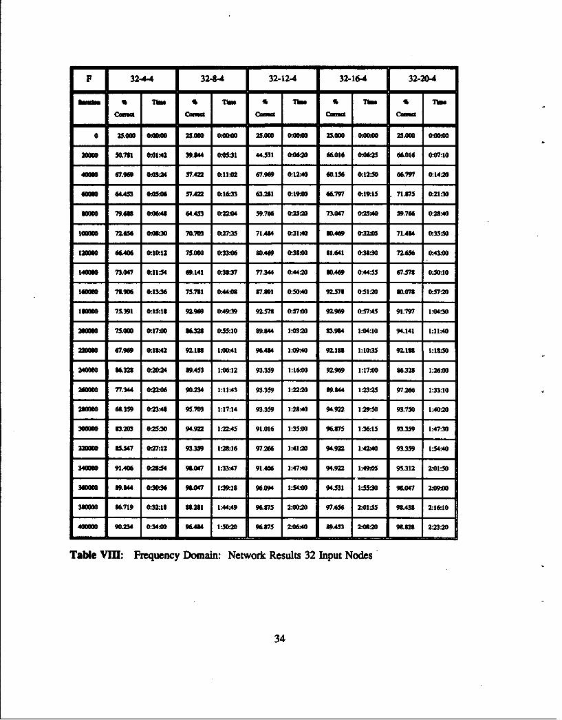
P 32-44 32-8-4 32-12-4 32-164 32-20-4

bItfts S TWO S T m Tro S TIM S IbW

Crat C*mg Cmma (Ct Cwmu

0 25.000 O:00 25.O 0:00300 23.000 o:0o0o 25.000 o0o 25.000 0:00:00

S50.781 0:01242 39.844 0:05.31 44.531 0:062 66.016 0.66 66.016 0:07:10

40000 C7.909 0:03:24 57.422 0.11W0 67.969 0:12.-40 0.156 0:12:50 66.797 0'14:20

am660 64453 0:05:06 57A22 0:16:33 63.281 0:19:00 66.797 0:!9:!5 71.875 0:.21:30

U06M0 79.6A 0:0)64 64.453 0:.22.04 59.766 0.25:20 73.047 0:2540 59.766 0:.2840

100000 72.656 0:66-30 70.703 0:.27.35 71.484 0:31:40 30.469 0:32:05 71.484 0:35:50

12060 6.406 0:1.0:.12 75.000 0:.33:06 0.4"9 0:31.:00 81.641 0:33:30 72.656 0:43.00

140000 73.047 0:11:54 0.141 0.38-37 77.344 0:44:20 30.469 0:44:55 67.57n 0.50:10

1600o0 71.906 0:13:36 75.781 0:.44.0 7.891 0.50:40 92.578 0:.51:20 30.078 0.57:20

130o00 75.391 0:15:18 92.90 0:49.39 92.578 0:57.00 92.969 0.57:45 91.797 1:04.30

200000 75.010 0:17:00 36.32 0-.55:10 39.344 1:03:20 83.984 1.04:10 94.141 IlA1.

220000 67.99 0:.18:42 92.13 1.00:.41 96.484 1.0940 92.183 1:10-.35 92.113 1-18:50

240600 36.328 0.20:24 9.453 106:12 93.359 1:16.'00 92.969 1:17.00 86.328 1:26.00

260M0 77.344 0:22. 90.234 1:11:43 93.359 1:22:20 99.844 1:23:25 97.266 1:33:10

230660 6K359 0:.23:48 95.703 1:17:14 93.359 1:21:40 94.922 1:29.50 93.750 !40:20

300M0 83.203 0.25.30 94.922 1:22:45 91.016 1:35.00 96.875 1:36:15 93.359 1:47:30

320660 85.547 0.27:12 93.359 1:23:16 97.266 1:41:20 94.922 1:42'40 93.359 1:54:40

340000 91.406 0"23.54 9L647 1:3347 91.406 1:47:40 94.922 1:49:05 95.312 2.01:50

34060 39.U44 0.30.36 93.067 139:.18 96.094 1:54:00 94.531 1:55:30 9(L047 2.09:00

331000 36.719 0:32:18 33.281 1:44"A9 96.V75 2:00:20 97.656 2.01:55 9.438 2:16:10

9M - - - -40 0.234 O:.M:W %640 1:.5" Mrs0 98 75 .- :40 89.A 2.'0:W20 MM82 2 212

Table VIII: Frequency Domain: Network Results 32 Input Nodes

34

53 OlMrvatlo.

The experiments show that either type of network can be used successfully to classify

radar signals. However, the acceptability of a network's performance depends on the application

and is usually defined as the ability of the neural network to achieve some threshold of success

over a set of test vectors. It is important to note that in general, neural networks cannot

guarantee a one hundred percent success rate for all possible inputs. (One of the networks in the

experiments (32-25-5) did achieve a success rate of one hundred, but this was on a limited set

of test vectors).

For example, if a 95 percent success rate is considered to acceptable, then the time

domain networks: 16-20-5, 16-25-5, 32-15-5, 32-20-5, and 32-25-5 all pass this criterion based

on the set of test vectors presented to them. In the frequency domain, the networks: 32-8-4, 32-

12-4, 32-16-4, and 32-20-4 meet this criterion. However, if the application calls for a 99 percent

success rate than only the time domain networks 32-15-5, 32-20-5, and 32-25-5 can satisfy this

requiemnenL None of the frequency domain networks meet this standard.

The experimental results concur with Kudrycki's result that the number of nodes in the

hidden layer must be at least three times the number of nodes in the output layer to obtain

adequate performance. Apart from the frequency domain network 32-8-4, the highest rate of

success, for any of the networks having equal or double the number of nodes in the hidden layer

as in the output layer, was 91.406 percent. For the networks with only 16 input nodes, the

highest rating was 76.953 percent. Equal or better performance is obtained from networks whose

hidden layer had four or five times the number of nodes in the output layer. This greater degree

of success, however, was achieved at the cost of additional training time. It should also be noted

that these larger networks cannot execute as fast as the networks with fewer connections, (unless

parallel processing techniques are employed).

The training time was found to be proportional to the number of connections in the

network and in all cases fairly lengthy. The times shown in Tables III, IV, VII, and VIII indicate

only the training time, and yet this alone adds up to more than 30 hours. This total does not

include the time required to generate the training and test vectors, the time to build the networks,

the time to run the tests, nor the time to record the results. The entire process actually required

35

maee than two persm-weeks. However, to achieve the same results using traditional programming

medtods would require many times this effort. Of course, if one decides in advance of the

training process that a certain percent success rate is acceptable, then the training time can be

reduced by stopping the training process when this level of success has been met. One still needs

an upper limit, as the success rate may never reach this level. In the experiments performed in

this project, the number of iterations of training (400,000) was chosen arbitrarily on the

assumption that if the training error function had failed to converge after this amount of training,

then it was unlikely to ever do so. The reader will note that even after 400,000 iterations of

training, 8 of the 20 networks had failed to reach the 95 percent threshold.

In comparing the general performance of the two types of networks it is clear that the

time domain networks were the better performers. Taking a 95 percent success rate as the

acceptable performance criterion, two of the 16 input time domain networks 16-20-5 and 16-25-5

were able to achieve this rate, whereas the highest success rate of all of the 16 input frequency

domain networks was only 76.953. To achieve this level of success in the frequency domain

requires a 32 input network. This is significant because it is generally easier to generate data for

networks with smaller input vectors, and networks with fewer connections result in faster

execution times. The actual time required to obtain the 95 percent rate for the time domain

network 16-20-5 was 55 minutes and 30 seconds, whereas one hour, 17 minutes and 14 seconds

was required to achieve this rating for the frequency domain network 32-8-4. Note also that in

the frequency domain case, additional time is required to perform the required transformations

in generating the training and test vectors. The poorer performance of the frequency domain

networks could be a result of the Blackman window transformation. The distortion of the input

data caused by this transformation could increase the similarity between two modulation pattern

types thereby decreasing the network's ability to distinguish between the two different patterns.

6.0 CONCLUSIONS

This paper has described the fundamentals of neural networks: their construction,

training, and behaviour. Particular attention has been payed to the class of neural networks called

back-propagation networks due to the simplicity of their training algorithm and their

36

effe tiveness in solving classification type problems. Theoretical issues involving the

arcitect, re, training algorithm, the execution algorithm, and several methods for accelerating the

taning process of this class of neural networks were covered. Practical consideration were dealt

with as well. These include the pre-treatment of input datm, initialization of weights, the choice

in the number of training vectors, the number of layers and the number of nodes in each layer.

This background material was then followed by a description of a series of experiments

which investigated the applicability of the neural network technique in classifying the modulation

paterns of pulse-to-pulse frequency agile emitters. The experiments showed that it is possible

to construct a neural network to perform this classification task. They also showed that there are

no clear-cut rules to follow in the construction of a network. It is somewhat of a black art -

one must rely on rules of thumb and "tweaking" to produce a successful network.

As well, the experiments showed that several networks with different architectures could

be trained to perform the same task successfully. In designing a particular neural network for

a specific application, one is generally forced to make a trade-off between network performance,

training time, and execution time. To find the optimal network, the designer must experiment

with different architectures and differnt representations of the input data. This can be a time

consuming task, involving the construction, training and evaluation of multiple networks. These

tasks are relatively simple ones, certainly much simpler than implementing a classification

algorithm in software. The problem of classifying the five signal patterns used in this project,

a problem easily solved by a human, is actually very difficult to solve using traditional software

techniques, particularly when the inputs are allowed to vary as much as they do in this project

(variable number of inputs and periods with arbitary phase).

Finally, neural networks are a promising technology for radar signal classification

problems. However, more experimentation is required. For example, to test performance when

there is a greater variability in the possible signal data. This project also made restrictive

assumptions concerning the nature of the signal data, eg., fixed PRI, a minimum of eight pulses,

and at least one full period of the modulation pattern per illumination. While it is true that any

technique will have difficulty classifying a signal with less than eight pulses and only a fractional

portion of one modulation pattern, an effective classifier must be able to handle signals exhibiting

PRI agility.

37

7.0 REFERENCES

[1] J.A. Andeson, Radar Signal Categorizadox wing a Newal Network, Deparment ofCopitive and Lnguistic Sciences and Department of Psicholo, Brown University,Providence, RL (Septmber 1988).

[2] I.L Coat & P.CJ. Hill, 77e Application of Neural Networks to Radar Class#kction, IEEElectrom Division Colloquium on Elecutnic Waufwe Systems, (January 1991).

[3] A. Brown, Neural Networks in Naval Electronic Warfare Claoficadon Problems,Crleton University, Ottawa (1990).

[4] J.A. Freeman & D.M. Skapura, Neural Networks, Algorithms, Applications, andProgranuning Techniques, Addison-Wesley Publishing Company Inc., Reading, MA(1991).

[5] D. Fukunaga, Introdueion to Statistical Pattern Recognition, Academic Press, New York,NY (1972).

[6] G. Hinton, Neural Networks for Indiist'y, Department of Computer Science, Universityof To•nto, Toronto (December 1991).

[7M V. 0ilmasauskas, J. Guiver & F. Pelton, NeuralWorks Porfessional II: User's Guide,NeuralWare, Inc. Pittsburgh, PA (1989).

[81 R.P. Lipmann, An Inxrodu ton to Computing with Neural Nets, IEEE ASSP Magazine,(April 1987).

[9] R.P. Lipmann, Pattern Classification Using Neural Networks, IEEE CommunicationsMagazine, (November 1989).

[101 A. Maron, C. Hmt & R. Pap, Handbook of Neural Compuing Applications, AcademicPress Inc., San Diego, CA (1990).

[111 A.V. Oppenheim & R.W. Schafer, Discrete-Tbne Signal Processing, Prentice-Hall, Inc.,NJ (1989).

[12] W.IL Press, B.P. Fiannery, S.A. Teudolsky & W.T. Vetterling, Numerical Recipes in C,The Art of Scientific Computing, Cambridge University Press, Cambridge, MA (1988).

[13] D.E. Rumelhart, J.L. McClelland and the PDP Research Group, Parallel DistributedProcessing, Exploration in the Microstructure of Cognition, The MIT Press, Cambridge,

38

MA (1986).

[14] G.B. Wiliaom, Radar Cln using a Neural Network, SPIE Vol 1294 Applicaziomof Ardfca Neural Networks, (1990).

39

Appenix A: Figures of Experimental Results

A-1

Tme 16-5-5 Training time

10000

90-- - -- - -- - --- - - - - -

50 ........40 . . . . . . . . . . . . . . . . . . . . . . . . . . . .

Ow .............................

2000----------------------------1000--------------- -- - - -- -

0

0 100 200 300 4W0Training Iterations (000)

FTmure 5: 165-5 Rrasult

A-2

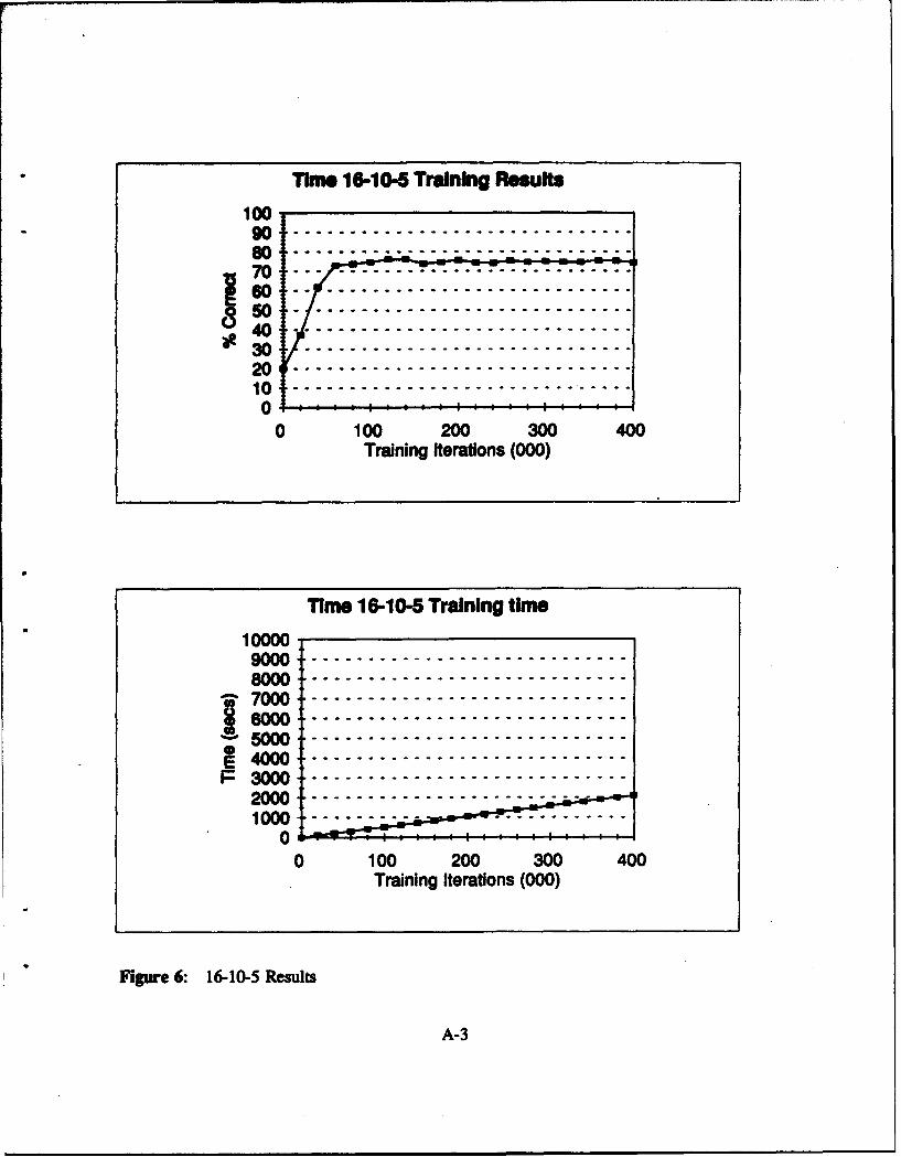
Time 16-10-5 Tradnlng Rsufts

100

s . o e o ... . . .. . .. . ... .. . • o. . •. !.. . . .7 0 . . . . . . . ..-- - ". ..-. ._._ '. .- - " ' _ . . . . .

10 . ........................ "....40 ---- ---------- ---------------- : :

00 100 200 300 400

Training Iterations (000)

Time 16-10-5 TraIning time10000

7000---------- ------7000 -----------------------------

I GO G -o -•-°-. . -- °

5 000 -------------------- --- -----

E 4 00 0 - - - - - - - - - - - - - -P 3000 --- - - - - - - - - - - - -

2000-------------1 0 0 0.....----............-

0 100 200 300 400Training Iterations (000)

Figure 6: 16-10-5 Results

A-3

Time 16-15-5 Training Results

100

0 100 200 300 400Training Iterations (000)

Time 16-15-5 Trainlng time

10000

0... .........................T0i..... .................

70 0----- - ------------------

%5000-------------------------4

~400.. ...........................Sp300--------------------------

1000.......................-------

0 100 200 300 400Training Iterations (000)

~Time 7:-5- Tra15-g Resule

100A04

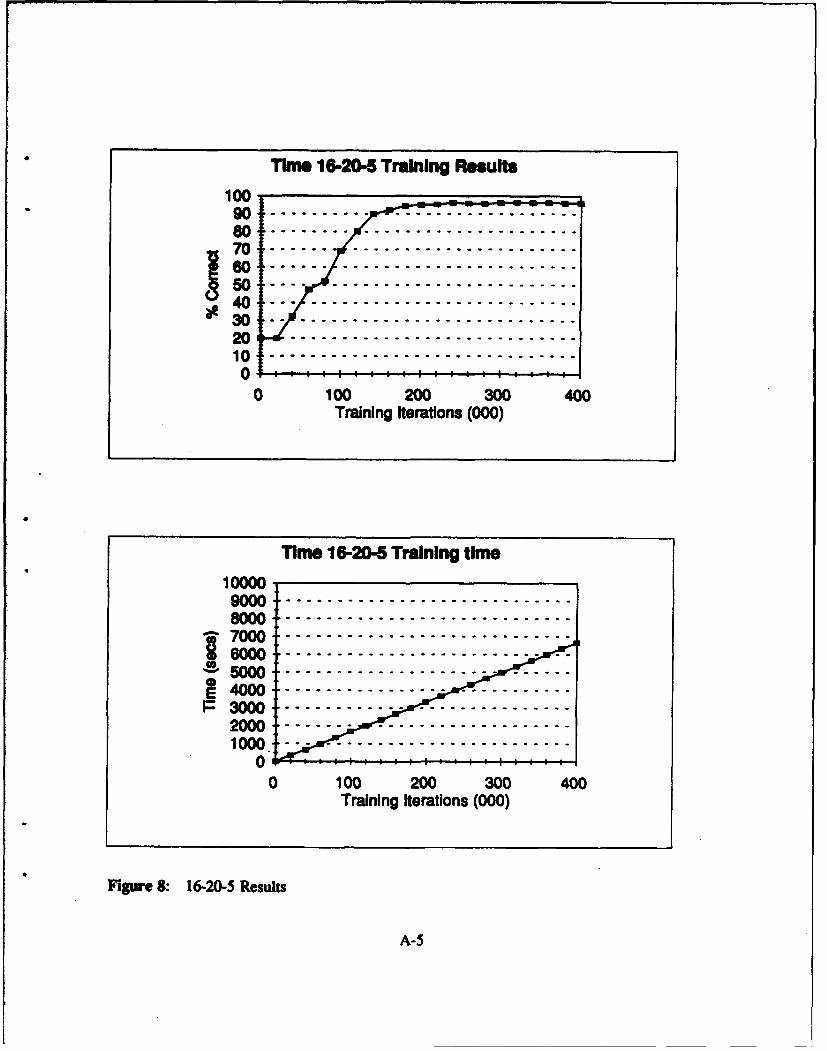
Time 16-20-5 Training Results

100

90 ---- --- : ---------- :

s ...... .......................SO . . . °. . . .. .. ...... ..........

40 - - - - - - - - - - - - - - - - - - - - - - - - - - - - - -. ° . .

30 - - - - - - - - - - - - - - - - - - - - - - - - - - - --° . . . . . .

20 ..............................10 - - - - - - - - - - - - - - - - - - - - - - - - - - -: : :

0 100 200 300 400Training Iterations (000)

Time 16-20-5 Training time

700 ..................... .... ...

10000 0 30 0n I--------------------- ------8000----------------- ----------

P 3M000------------ --------------2M OO--------------------------1000--------------------------

00 100 200 300 400

Training Iterations (000)

Figure 8: 16-20-5 Results

A-5

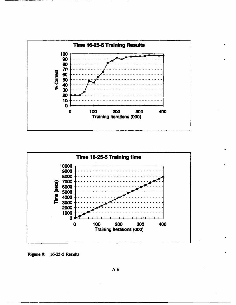
Tim 16-25-5 Training Results

100.190 .. . . . ..... --- - --.--

60 .. .. .. ...... ...... .....7 0 1 0 0 2 0 0 -- -0 0-- - 4 00- -

Training Iterations (000)

Time 16-25-5 Training time

10000

3700----------------------------

160....... g.... •.... •....

2000.........................10 0 0--- - -- - - - - - - - - - -

0 100 200 300 400Training Iterations (000)

Figur-e 9: 16-25-5 Results

A-6

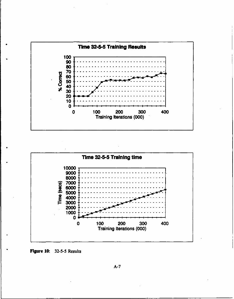
Time 32-5&5 Training Results

10090 - - ----------------------------8 0O --- - - - - - - - - - - - - -70 ---- --- -------°°- °. . .-------------

20so . . . . . . . . . . . . . . . . . . . . . . . . . . . . .

00 100 200 300 400

Training Iterations (000)

Time 32-5-5 Training time

10000

O OO --- - °-- - - - - - - - - - - - - - - - - - - - - - - - - - -

71222.....................000 ----------------------------

2000E24000--------------------------P 3000 -----------------------------

2000-----------------------------1000 . . -. . . . . . . . . . . . . .

00 100 200 300 400

Training iterations (000)

Figure 10: 32-5-5 Results

A-7

Time 32-10-5 Training Results

0 100 200 300 400Training Iterations (000)

Time 32-10-5 Training time

10000

O O O . . - - - - -. . . . . . . . . . .... . . . . . . .900-----------------------------

000 - ----------------------------

7000---------------------------20 60---------------------------lov -------------------------o4000------------------------I

0 100 200 300 400Training Iterations (000)

Figure U1: 32-10-5 Results

A-8

Time 32-15-5 TraIning Results

0100. 20 300-w 400-

1O0009000 - -°- --- .... ............. ....

40-O

20-O

801• .. . . . •...... . . . . . . .

10 --- - - - - - -40 -- I : . I : -- - - - - - - - - - - - -

0 100 200 300 400Training Iterations (000)

Time 32-15-5 Traning time

10000A

63000 ----------------------- ------2000- ----------------- ----------

1000 -- -- - - - - - - - - -0

0 100 200 300 400Training Iterations (000)

FIgure 12: 32-15-5 Results

A-9

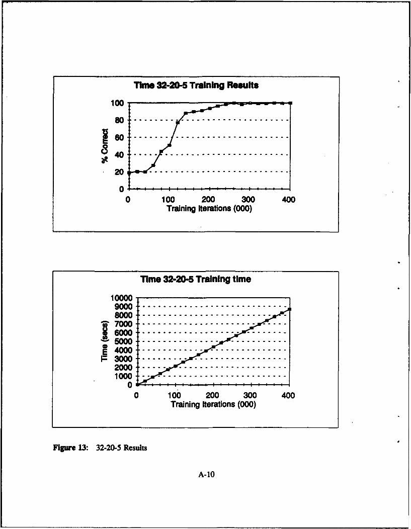
Time 32-20-5 Training Results

100

80-se o -- - - - - - - -- - - - - - - -

40-

20

0 • I: : : I

0 100 200 300 400Training Iterations (000)

Time 32-20-5 Training time

100007000 -.-.- --------- -------- - --...

00 00.......... -Tr000..... .ter.tions (000

20=00............................1000............................-

00 100 200 300 400

Training Iterations (000)

Figure 13: 32-20-5 Results

A-10

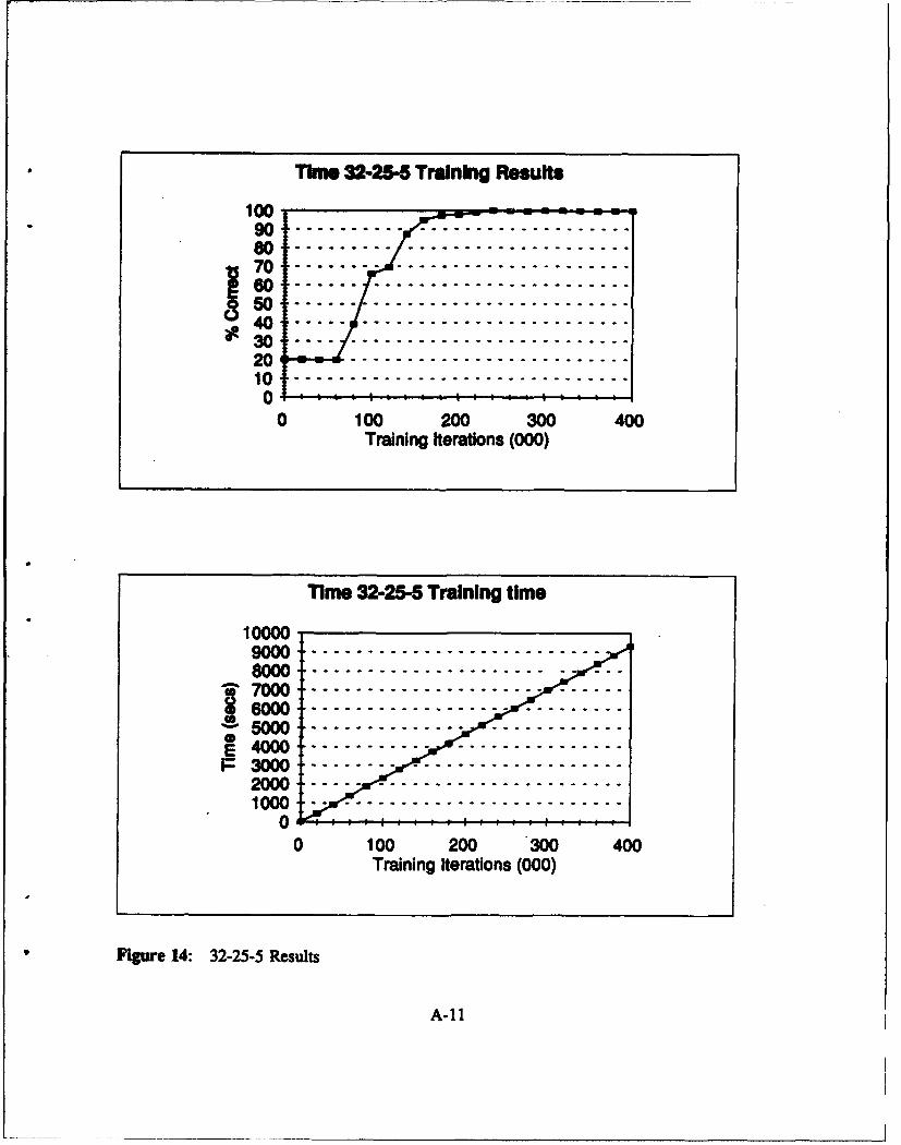
Thne 32-25-5 Training Results

100

o ............................

4 0 ---- --- --- --- --- --- ---

20- - - - - - - - - - - - -10 - - - - - - - - - - - - - - -0 'ti -* ! '

0 100 200 300 400Training Iterations (000)

Time 32-25-5 Training time

10000A

700 100 200-------- 300-400

3000Taiin iteration (000)-------

Figure 14: 32-25-5 Results

A-11

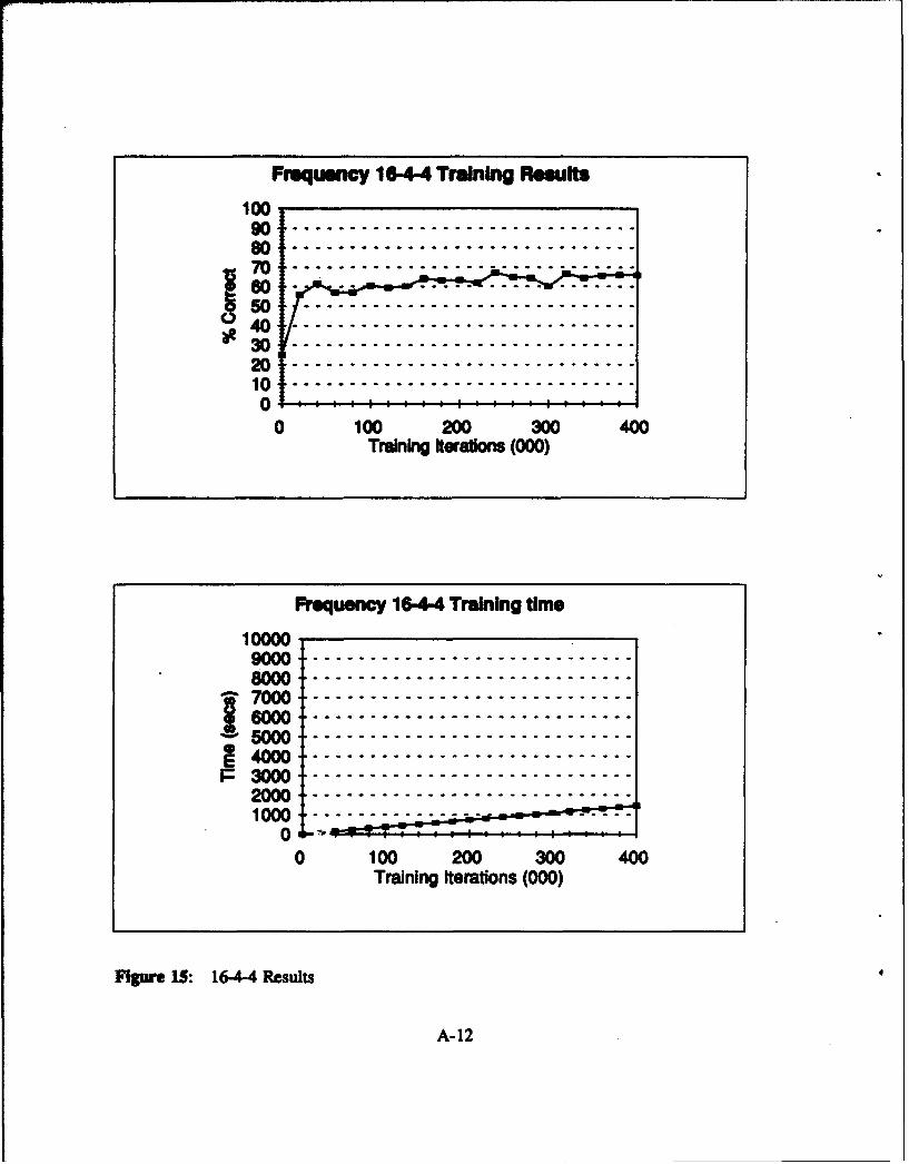
Frequency 16-4-4 Training Result

100

90 ---- ---- ---- ---- ---- ----

70 100-- - - -- - - .00..00 ..0

% 00.............................40 -- e ---------- -------- --------

70 .............................

' 150 0 --- - - - - - - - - -

0 100 200 300 400Training iterations (000)

""1uency 16-4-4Trning4time

10000.9000 -- •--- - --------------- °-------

8000 --------------- --- -----------

7 0 ... ..........................

20 0 --- --- --- --- --- --- ---

Traning Iteratons (000)

Ingre 15: 16-4-4 Reult

A-12

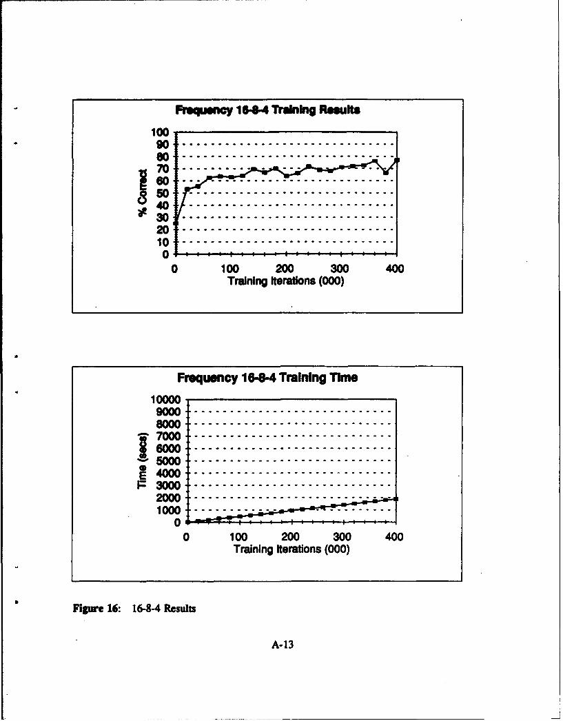
Prequncy 16-84 Training Results

60 .111 .........................

0 100 200 300 400

Traning Ierations (000)

Frequency 16-8-4 Traning Time

10000000 -------- ----- -- ------- --

000 ------ ------------- ---- ----

230 0 --- - - - - - - - - - - - - -

1 0 0 0---- ----------------------

0 100 200 300 400Training Iteratons (000)

Figure 16: 16-8-4 RasulTs

A-13

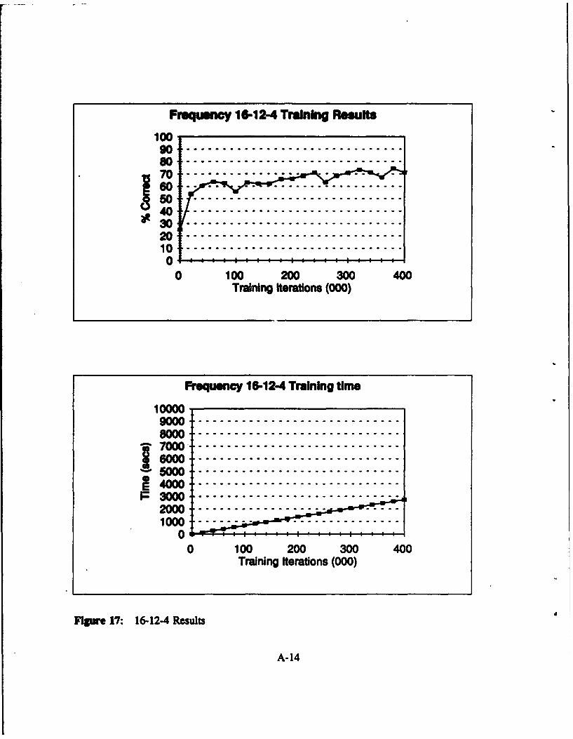
Frequency 16-12-4 Trainig Rsults

100

S................. . . . . . .

50 --u--------- ------------10 ..............................

0 100 200 300 400Training Iterations (000)

Rrequency 16-12-4 TrainIng time

100009000 --------------------------8000--------------------------

24000 ----------------------------

PF3000-----------------------------2000-WO-----------------1000 .p.w

00 100 200 300 400

Training Iterations (000)

Figure 17: 16-12-4 Results

A-14

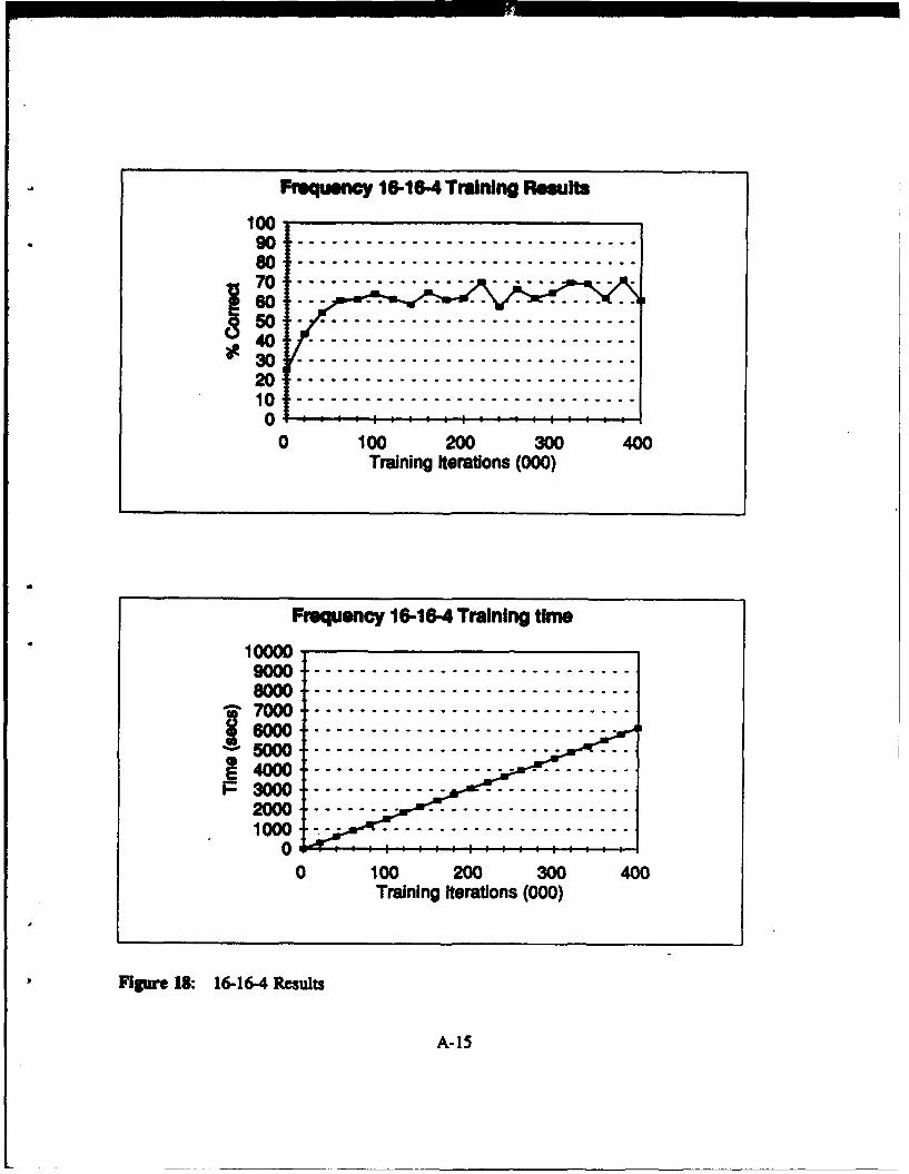
Frequency 16-16-4 Training Results

100

70 m.... ....... . ° ...... q

o o - ° -- - -° - . . . . . . . . .. . . . . .

0 -:: - I-I- :-: - : " : 1- : -- -- ---

0 100 200 300 400Training iterations (000)

Frequency 16-16-4 Training time

80000 ....-.. .... ...... ..........S7000------------------------------

0 0 .-....... ................n5000 ---- .

~4000--- - - -- - - -- - -- - -F3000-

22000 0 --.............1000------ --- - - - - -

00 100 200 300 400

Training Iterations (000)

Fipnme 18: 16-16-4 Results

A-15

Frequeny 16-20,4 Training Results

100

60 - --- - - --- --°-°°°-**- -o*° °- -- - ----°*

50 . .............................

0 ---::-:--: :"::-: "::

0 100 200 300 400Training Iterations (000)

Frequency 16-20-4 Training time

10000

1-500........................... •

1000---- - - - - - - - - - - - - -

2 0 100 20 300 400

Training Iterations (000)

Figre 19. 16-20-4 Results

A-16

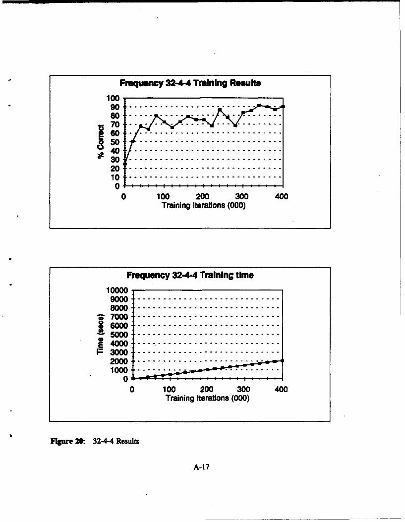
Frequency 324-4 Training Results

100

0 100 200 300 400

Training Iterations (000)

Frequency 32-4-4 Training time

10000

000 . °- - - - --... . - - °-.. . .. ..... . .. . . .. . ..

so .............. ......

4500-----------------------------D300-----------------------------2000----------------------------1000 - - - -- - - - - -- - - - -

0 100 200 300 400Training Iterations (000)

Frqune 20: 32-4-4 Restmts

A-17

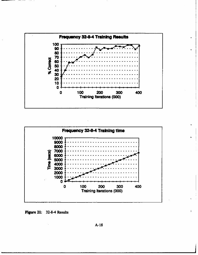
Frequency 32-8-4 Training Results

100

90 ---------•- - .-.....

73 0 --- - - - - - - - - - -

0 : 1: : :. al .i, , , : : : m A A A

0 100 200 300 400Training Iterations (000)

requency 32-4 Training time

10000.9000.............................-- -- -- -- --8000......................... -- - - -- --

7-'000.........................-

~4000............................ - - - -P3000............................ - - - -2=000............................1000 - - ----------------------

0 100 200 300 400Training Iterations (000)

FIgure 21: 32-8-4 Results

A-18

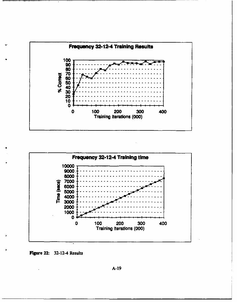
Frequency 32-12-4 Training Results

Training Iterations (000)

Frequency 32-12-4 Training time10000

000o -------- - -----------------

60= .... .................. .. .

s000 .-------------------------

F3000 ----------------------------

2000-----------------------------

1000 -------- ------ ------ ---- .

00 100 200 300 400

Training Iterations (000)

Figure 22: 32-12-4 Results

A-19

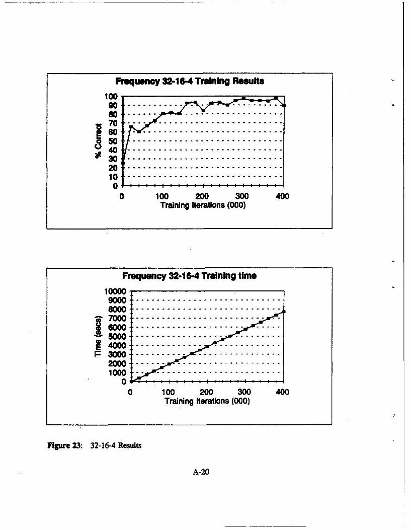
Frequenc 32-16.4 Training Results

8!2

Training Iterations (000)

Frequency 32-16-4 Training time

1O000

8000............... - - °............ -

p000............... - • -............ °

1000ng-trtins(00

Figure 23: 32-16-4 Results

A-20

Frequency 32-20-4 Training Results

100

90................

70 0

3600

850040..............................-*30..............................-

20..............................-10 .............................

0 100 200 300 400Training Iterations (000)

Frequency 32-20-4 Training time

10000

F3000............................---2000............................-1000..........................

600 100-- 200---- 300--400

2000Trinn Itertion (000)-- -- -- -- -

Figure 24: 32-20-4 Results

A-21

UNCLASSIFIED -63-UC ITV CLASIPICATION OF FORM

0hogst classification of Title. Abstract. Keywords)

DOCUMENT CONTROL DATA(Sowiuty eleaolfleakion of tit. lebody of ebstraft nd Wadexing amtot atioe mast be entered whei the overall docunwmw is 0asa4ie*

1. ORIGINATOR te imo and address of the orgaation preoling the document 2. SECURITY CLASSIFICATIONOra n for whom the documem w pelpred. e.. toisuimt sponsoring (overall security classification of the document.a conutul rs roemort tasking wo piy, weI i o in section L)including special wwning terms if applicable)DEFENCE RESEARCH ESTABLISHMENT OTTAWA

NATIONAL DEFENCESHIRLEY BAY, OTTAWA, ONTARIO KlA 0K2 CANADA UNCLASSIFIED

3. TITLE the compIlet document tift as indicated an the title page. Its classification should be indicated by the appropriateibrevinon (S.C or U) in parontheses after the tite.)

NEURAL NETWORKS FOR CLASSIFICATION OF RADAR SIGNALS (U)

4. AUTHORS Last mne, first name, middle Inital)CARTER, CHRISTOPHER, A. AND MASSE, NATHALIE (APPLIED SILICON INC.)

5. DATE OF Pt.UBLICATION bnmont and yer of publication of Ba NO. OF PAGES ftotel 6b. NO. OF REFS (total cited indecnantod containing information. include document)

NOVEMBER 1993 Annexes, Appendices. etc.)14

7. DESCRIPTIVE NOTES (the category of *h document. e.g. technical report, technical note or memorandunm If appropriate, enter type ofreport, e.g. interim. preoress. summry, annual or final. Give the inclusive dates when a specific reporting period is covered.)

DREO TECHNICAL NOTE

S. SPONSORING ACTIVITY (the name of the deportmnt project office or laboratory sponsoring the reserch amd development Include theaddross.)

DEFENCE RESEARCH ESTABLISHMENT OTTAWANATIONAL DEFENCER1ITRT.•V RAY. OTTAWA. ONTARIO KIA OK2 CANADA

9e. PROJECT OR GRANT NO. (if apprpiate, the applicable research 9b. CONTRACT NO. (if appropriate. the applicable number underand developmnt project or gran number under which the document which the document was written)

o0 rmwrit PlanSe specify whether project or gra-)

10a, ORIGINATOR'S DOCUMENT NUMBER (the official document 10b. OTHER DOCUMENT NO& (Any other numbers which maynunmor by which the document is identified by the originating be assigned this document either by the originator or by theactivity. This number must be nique to this docum ) sponsor)

DREO TECHNICAL NOTE 93-33

11. DOCUMENT AVAILABILITY (any iimitaions on further dissemination of the documem, other than those imposed by security classification)

(X) Unlimited distribution( Distribution limited to defence deprtments and defence contractors; further distribution only as approved

Distribution limited to defence deporments and Canadian defence contractors; further distribution only as approved( Distribution limited to government depetments and iencies; further distribution only as approved

D Distribution limited to defence depatments; further distribution only as approved( Other (plese specify):

12. DOCUMENT ANNOUNCEMENT (any limitation to the bibliographic announcement of this document. This will normally correspond tothe Document Avsil ty (11). However, where further distribution (beyond the audience specified in 11) is possible, a widerannouncement audience may be selected.)

UNLIMITED

UNCLASSIFIED

UECURITY CLASWIFICATION OF FORMOCM03 2106187

UNCLASSIFIED-64-__ _ _ _ _ _ _ _ _ _ _ _ _ _ _ _ _ _ _ _ _

UCWITY 0LASSIFICATION OF FORM

13. ABSTRACT I a Inst end ftcui 5vm- of do dbiemn. It my do am elewhere m the dody of the docuent itself. It is hqlydosi tie So *a st of ulasstfled doemients ble uclassified. Each wqrapO of e kbewoct shell beg with an indication of thesoeiy cl•uficoma of the Afoarmo in the pwapah tumless the dcunment itself is uaclauifie represanted as (S) (C). or U.It is net •scowy 0 itucludi here hxrcts i both officl hair s unless the text is bilimpi .

(U) Radar Electronic Support Measures (ESM) systems are faced with increasinglydense and complex electromagnetic environments. Traditional algorithms for signalrecognition and analysis are highly complex, computationally intensive, often relyon heuristics, and require humans to verify and validate the analysis. In this paper,the use of an alternative technique - artificial neural networks - to classifypulse-to-pulse signal modulation patterns is investigated. Neural networks are anattractive alternative because of their potential to solve difficult classificationproblems more effectively and more quickly than conventional techniques. Neuralnetworks adapt to a problem by learning, even in the presence of noise or distortion inthe input data, without the requirement for human programming. In the paper, thefundamentals of network construction, training, behaviour and methods to improve thetraining process and enhance a network's performance are discussed. As well, adescription and the results of the classification experiments are provided.

14. KEYWOROFS DESCRFTORS or IENTIM fteolmknic menmgfu torms or shan otr that ractlernze a dcumet and could behefu m eGuing the Dcument They saud bo seec Pid so de no securt cssiictiomn is requred. Identif•s such As euipmetmodel 401i0 ea1 . trode eiune, miliWY VOeWect cede name. 1eo9grphic location map also be included. If Possible keywords shuild be selectedfrom a published Uhesomi. e.g. Thesmaus of Engineerig and Scientific Terms (TEST) and that thwsmuus-identified. if it is not possible toselect indexing torns which are Unclessified, the clasification of eact should be indicated as with the title.)

NEURAL NETWORKRADARSIGNALPULSEMODULATIONCLASSIFICATION

UNCLASSIFIED

UCURITY CLASSIFICATION OF FORM