- 1 -

Mapping microphytobenthos biomass by non-linear inversion of visible-infraredhyperspectral imagesJean-Philippe Combe1, Patrick Launeau1, Véronique Carrère1, Daniela Despan1, VonaMéléder1,2, Laurent Barillé2, Christophe Sotin11 Laboratoire de Planétologie et Géodynamique, UMR-CNRS 6112, Université de Nantes,Faculté des Sciences et des Techniques, 2 chemin de la Houssinière BP 92208, 44322 Nantescedex 3, France2 Laboratoire d’Écophysiologie Marine Intégrée – ISOMer – UPRES EA 2663, 2 chemin de laHoussinière BP 92208, 44322 Nantes CEDEX 3, FranceE-mail of corresponding author: Jean-Philippe.Combe@chimie.univ-nantes.fr

AbstractThis study presents an innovative approach to map microphytobenthos biomass and fractionalcover in Bourgneuf Bay (French Atlantic coast) using Digital Airborne Imaging Spectrometer(DAIS) hyperspectral data. Microphytobenthos is a microalgae forming a biofilm on themudflat. Its spatial distribution is heterogeneous so it varies on a finer scale than that ofairborne instrument spatial resolution, leading to a “mixed pixel” problem. Moreover, somemicrophytobenthic species form, at low tide, a biofilm deposited at the surface of thesediment substrate. The resulting signal is a highly non-linear combination of spectralendmembers due to microscale intimate mixtures. This prevents the use of classical linearunmixing models to retrieve biomass from reflectance spectra. A Modified Gaussian Model(MGM) is therefore used to remove the effects of surface roughness, shadowing and any otherunknown processes that contribute to the overall shape (continuum) of the reflectance spectra.Then, relationships between microphytobenthos biomass and spectral shapes are derived froma spectral database compiled from laboratory reflectance spectra of microalgal monospecificcultures with different biomasses. Finally, microphytobenthos biomass and fractional coverare retrieved from the DAIS image by comparing the reflectance spectra of each pixel to alibrary of synthetic spectra corresponding to combinations of various biomasses and substratepercent cover. This new approach, when compared to more classically used ones such asindices, linear unmixing or spectral distance analysis, is proven to enable a much morereliable determination of biomass despite the large variety of substrates found in BourgneufBay.

Keywords: imaging spectroscopy, reflectance spectroscopy, microphytobenthos, biomass,Modified Gaussian Model, continuum, spectral library, mapping

1. IntroductionFor many environmental studies, surface material identification is the first step in eitherbiological or geological applications. Observations, quantitative measurements andcomparisons often need to be performed on a large number of samples on areas of severalsquare kilometers. Remote sensing provides synoptic views that are useful tools for suchanalyses. Furthermore, this approach is compatible with mineral and organic surfacecomposition analysis as it can be performed remotely by spectroscopy in the visible andinfrared domains.The objective of the present paper is to estimate the spatial distribution of microphytobenthosbiomass from a hyperspectral image of Bourgneuf Bay (French Atlantic coast) acquired bythe Digital Airborne Imaging Spectrometer (DAIS). This requires the ability both todistinguish vegetation species and to quantify the biomass of a specific taxon or ecologicalgroup such as microphytobenthos. In coastal ecosystems, this is becoming essential to derive

- 2 -

material fluxes (Guarini et al., 2000). It is especially true in the case of Bourgneuf Bay, amacrotidal shellfish ecosystem with a large mudflat, where microphytobenthos is thought tobe a major food source for cultivated oysters (Cognie et al., 2001) (Figure 1 and Figure 2 a).Microphytobenthos is composed of benthic unicellular phototrophic microorganisms, mostlydominated by pennate diatoms (Paterson and Hagerthey, 2001). Studies suggest thattaxonomic discrimination and biomass quantification are possible in situ (Guillaumont et al.,1988; Paterson et al., 1998) in the 400-1000 nm range of spectral absorption of vegetationpigments. However, in the vicinity of rocky areas, the benthic microalgal biomass has to bedetermined in the presence of macroalgae. Imaging spectrometry would therefore provide anopportunity to map the spatial distribution of microphytobenthos biomass: accuratecomponent determination is expected due to high spectral resolution and continuous spectralsampling (Richardson, 1996; Richardson et al., 1994).However, quantification is difficult due to the spatial distribution of microphytobenthos atmacroscale and the non-linearity between biomass and radiometric absorption. The complexinteraction of radiation with biomass is mainly due to surface structure: microphytobenthosdevelops at low tide at the surface of illuminated sediments, forming a partially transparentbiofilm. Such an intimate mixture always results in complex light paths between purecomponents, so they cannot be resolved by a linear model of unmixing (Adams, 1993; Gross& Schott, 1998; Richards & Jia, 1998). Since reflectance does not follow a simple relationshipwith biomass, each pattern of biofilm density can be considered as an endmember.The other key point concerns the spatial distribution of microphytobenthic biomass,characterized by patchiness (Paterson and Hagerthey, 2001; Méléder et al., 2003). Accordingto Saburova et al. (1995), patches extend about ten centimeters and form aggregates, the sizeof which varies up to about ten meters. Consequently, the spatial scale is often finer than thatof the ground instantaneous field of view of the remote sensing instrument (field, airborne orspaceborne). This spatial heterogeneity results in a “mixed pixel” problem. In the literature,Spectral Mixture Analysis (SMA) is often found to be more powerful than indices for mixturedeconvolution (McGwire, 2000; Dennison, 2003). However, in order to obtain coefficientswhich can be assimilated to fractions, accurate endmember selection is required that caneither be intimate mixtures or pure components (Tompkins, 1997). For instance, the spatialdistribution of microphytobenthos biofilms at the surface of the mudflats and their localconcentration are two independent variables. This is the main argument for methodologicaldevelopment.At microscale, surface interactions with light are modeled by radiative transfer theory(Chandrasekhar, 1961) in which atmospheric backscattering, illumination and viewinggeometry, and surface properties (Hapke, 1981) are taken into account. For example, spectralfeatures from adjacent surrounding materials outside the field of view may be added (Sanderset al., 2001) when atmospheric scattering changes the optical path. However, radiativetransfer equations require both measurement of grain sizes and the optical constants of thedifferent materials, and these are not easily available. An alternative and direct method is totake spectra of samples for which the composition and structure are known. In our case, arelationship between biomass and radiometry can be determined by building a spectral librarybased on microalgal monospecific cultures. Moreover, various substrates (e.g. sand, mud,etc.) can be taken into account by field acquisitions. Spatial heterogeneity can then bemodeled by computing spectral mixtures of known biomasses and various substrates.For quantification, only absorptions must be used. This requires the removal of contributionschanging albedo and slopes due to other absorbing (or emitting) materials (Clark et al., 2003).This is commonly described as a part of the continuum that can be modeled by mathematicalfunctions like straight lines, polynomial or Gaussian curves, etc. (Clark and Roush, 1984). Onthe target itself, another part of the continuum may be due to absorption processes that are not

- 3 -

related to the mineralogical composition, like scattering and shadowing by surface structures(Hapke, 1981, Clark and Roush, 1984). As an example, the center of spectral features can beshifted by a tilt of the global slope. Consequently, it is important to remove the continuum toretrieve the true absorptions. This is even more crucial in this study for the comparisonbetween field or image data and library spectra. Commercial software for spectral analysislike ENVI (Environment for Visualizing Image, RSI ©) offers a fast and easy continuumremoval procedure, which divides a straight line inside a user-defined wavelength domain.This has already been used by Carrère (2003) and Carrère et al. (2004) to map and quantifymicrophytobenthos. More generally, on vegetation spectra, de Jong (1998) and Rowan et al.(2000) have presented an application for green canopy in the 600-2500 nm and 550-715 nmrange respectively. Many examples are found in the literature, especially for mineralendmember retrieval by the Tetracorder algorithm (Clark et al., 2003). Although this methodhas been extensively used, this continuum is often sensitive to absorption features. This isbecause it is based on local maxima of reflectance in a given wavelength domain (chosen bythe user). Consequently, reference points often correspond to the shoulders of deep absorptionbands, but that does not mean these locations are free of small absorptions. Moreover, theresulting continuum is composed of linear segments that are difficult to explain physically.Among processes causing a continuum, scattering by rough surfaces or atmospheric particlesgives a monotonic function like a reddening in the visible (Börner, 2001; Erard, 2001; Secker,2001). A better function to model this trend should be derivable, simple (with two or threeparameters) and based on a wavelength range without absorption bands.A decomposition with Gaussian curves fitting all absorption bands in logarithmic reflectanceplus a straight line function in wavenumber (Modified Gaussian Model or MGM, by Sunshineet al., 1990) is able to compute such a single continuum shape, independently of individualabsorptions. In this work, a spectral continuum is estimated by MGM and removed both oneach pixel of the image and on each member of the library, to minimize all spectralcomponents other than absorption features of interest. Quantification from the image is doneby pairing each pixel with a mixture from the library presenting the closest spectral pattern inthe range 496-727 nm and for which the corresponding biomass value is known in detail(effective biomass and patch spatial distribution). Available results provide biomass maps andfractional cover of each component.

2. Site description and image characteristics

2.1. A case study: benthic microalgae in a coastal zoneSpectral analysis of microphytobenthos was the basis for the development of a methodology.Interdisciplinary work with marine biologists and the HySens European program provided theopportunity to acquire a hyperspectral image of a macrotidal bay on the French Atlantic coast.

Site overview

Bourgneuf Bay is located south of the Loire estuary (46-47°N, 1-2°W). It is a shellfishecosystem, where a large part of the tidal flat is used for oyster culture. This bay ischaracterized by high turbidity levels ranging from 4 to 415 mg.L-1 of suspended particulatematter for daily average values (Haure et al., 1996), with maximum values reaching 1 g.L-1

during spring tides. Like in Marennes-Oleron Bay situated 100 km to the south, this turbiditylimits phytotrophic primary production in the water column (Guarini, 1998), which suggeststhat benthic microalgal production has a key role in such ecosystems.

Surface description

At low tide, the sequence of the materials encountered from the beach to the seawater is

- 4 -

representative of the ecosystem. The dry and bright sand at the top level of the beach is thefarthest point with respect to sea level. Most of the fine-grained sand is transported by thewind and not directly by the water. It is an area with low cohesion. The upper limit reached bythe sea at high tide is characterized by a more cohesive surface where waves can build ridgesand runnels. Depending on the time elapsed since the last tide and the local weather, thesurface is either wet or dry. Pieces of macroalgae are often left behind by the tide.Microphytobenthic epipsammic (sand-dwelling) species can sometimes be found at thesediment surface but they do not constitute a biofilm. In Bourgneuf Bay, the extension of thesand is limited by mudflats, which are water-rich sediments with very low cohesion. Epipelic(mud-dwelling) microphytobenthos species are adapted to this substrate and form biofilmsthat represent the largest proportion of the biomass. Sediments typically range from sand (63– 2000 µm) to mud (< 63 µm). A detailed description of the study area and the environmentalconditions can be found in Méléder (2003).To summarize, several kinds of material can be found in Bourgneuf Bay with a centimetricspatial variability while the spatial resolution of the available hyperspectral DAIS image isabout five meters. This difference in spatial scale led to our investigation of how to retrievethe spatial content of a given pixel. This study is presented in section 1.4.

Figure 1. Synoptic view of the intertidal zone of Bourgneuf Bay and the location ofcomponents.

Figure 2. Surface types of Bourgneuf Bay – a. View of the bay: a microphytobenthosbiofilm is in the foreground. A few meters farther away, outcropping rocks correspondto an ancient oyster bed and the sea is in the background. Spectra acquisition and in situbiofilm sampling is illustrated in the foreground – b. Examples of GER 3700 fieldspectra.

2.2. The DAIS hyperspectral data

Data acquisition

The bay was imaged by the Digital Airborne Imaging Spectrometer (DAIS) in 2002 duringthe European Hyperspectral Sensor (HySens) airborne campaign (Figure 3). The instrumenthas 80 channels, covering the 500-12600 nm spectral range: 72 from 496 to 2412 nm, 1 in theMid-Infrared (MIR) and 6 in the Thermal Infrared (TIR). The spectral domain used here,between 496 and 1035 nm, corresponds to 32 channels of the imaging spectrometer DAIS(first spectrometer) and 323 channels of the GER field spectrometer. Flight conditions werechosen for a spatial resolution of around 5 m. In situ reflectance spectra were acquiredconcurrently with the overpass to help validate image calibration with surface reflectance. Abright and a dark target were used: dry sand on the upper beach and water respectively (seeFigure 3 for location). The flight occurred under suitable atmospheric conditions; highvisibility, a stable atmosphere and low humidity.

Figure 3. Bourgneuf Bay DAIS image (RGB colors associated with channels at 496, 675and 798 nm respectively). Green: microphytobenthos; light red: terrestrial vegetation;dark blue: macroalgae; white: sand; gray: mud; blue: water.

Calibration

Atmospheric corrections were performed by DLR (Deutsche Zentrum für Luft-undRaumfahrt), using the ATCOR 4 algorithm (Richter, 1996). Bright and dark reference targetswere used to better adjust the image to field reflectance. With such good atmospheric

- 5 -

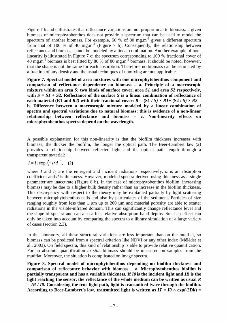
conditions and with no topographic or shadow effects over the area of interest, calibrationprovides good results as can be seen by comparing airborne spectra and field spectra (Figure4). In both cases, the spectrum of dry sand corresponds to the reference homogeneous brighttarget. Since the maximum difference is less than 4.5 %, instrumental calibration andatmospheric corrections are satisfactory.

Figure 4. Validation of the calibration process on a homogeneous sandy area: nosignificant difference is seen between the field GER 3700 spectrum and the airborneDAIS spectrum.

2.3. Reflectance spectraReflectance spectra of every component that can be present within a pixel (Figure 2 b) weremeasured in the field with a GER 3700 hand spectrometer (Figure 2 a). Microphytobenthos,mud, wet sand, macroalgae and water can be mixed together. Dry sand and terrestrialvegetation are not expected to be in close contact with microphytobenthos but are present inthe scene. Surface reflectance was determined by first measuring the light reflected from acalibrated white reference panel (Spectralon) and then the light reflected by the sedimentsurface.In Figure 2 b, microphytobenthos, macroalgae and grass field spectra show a similar red edgebetween 680 nm and 750 nm, characteristic of vegetation, but very different levels of theInfrared (IR) plateau, due to differences in light scattering. Sediment spectra have a simplemonotonic shape with a positive slope because mineralogical absorptions do not occur in thisrange and surface reflectance depends mostly on grain size. Sediment water content affectsthe total level of reflectance because water strongly absorbs light in the IR spectral domain.To avoid the influence of viewing geometry and illumination effects, we chose also to acquirespectra of microphytobenthos cultures in the laboratory.The calibration of the microphytobenthos reflectance spectra to their quantity of biomass wasperformed by Méléder et al. (2003). Microphytobenthos biofilms were simulated by slowlyfiltering diatom cultures on fiberglass filters. Then, reflectance spectra were acquired (Figure5) before diluting pigments in solvents (see Méléder et al., 2003, for details). Among thepigments measured by High-Performance Liquid Chromatography (HPLC), only chlorophylla concentration in mg.L-1 is used to evaluate a biomass in mg.m-2 (amount of chlorophyll afound on each synthetic biofilm). A look-up table of biomasses is then attached to the spectrallibrary of microphytobenthos biofilms.

Figure 5. Microphytobenthos reflectance spectra of 15 monospecific diatom cultures ofincreasing concentrations deposited on a fiberglass filter substrate (Méléder et al., 2003).

The substrate, a fiberglass filter (Figure 5), gives spectra with fundamentally different shapescompared to measurements on natural samples taken on the mud (Figure 2) because thebiofilm is partially transparent. Consequently, further corrections, as explained in section 1.4,are needed in order to compare data from different sources.

2.4. Spectral mixtures

Correction for inter-data comparisons

Any microphytobenthos spectrum (Figure 6 a) is the result of a combination of substrate andbiofilm contributions because incident light is partially transmitted through the total thicknessof the biofilm and then can be reflected by the substrate (Figure 6 b). The measured emergentradiance ITRT is written as:ITRT = I0 × TB

2 × RS (1)

- 6 -

where I0 is the incident radiation, IR the reflected radiation, TB the transmittance through thebiofilm and RS the reflectance on the substrate. One can note the non-linear combination ofbiofilm transmittance TB and substrate reflectance RS in the product TB

2 × RS. Let RM0 be thereflectance of microphytobenthos biofilm on a glass microfiber substrate (with reflectanceRS0) measured in the laboratory then RM0 = IR / I0 = TB

2 × RS0. When the spectrum RS0 of thesubstrate is known (Figure 6 a), the microphytobenthos component TB

2 of the measuredreflectance spectrum RM0 can be retrieved by TB

2 = RM0 / RS0 (Figure 6 c). Inversely, field orimage emergent light is modeled by ITRTn = I0 × TB

2 × RSn, where RSn is the reflectance of thenatural substrate, typically mud or sand in our case study (Figure 6 d). This step is necessarybecause residual chlorophyll a (i.e. not linked to living organisms) is contained in sedimentsand causes a small but significant absorption at 675 nm. In addition, for an absolutequantification, biomass spatial distribution within a pixel and biomass density must be takeninto account as described below.

Figure 6. Principle of an intimate mixture between microphytobenthos biofilm and itsmineral substrate and the obtaining of synthetic microphytobenthos spectra. – a.Measured spectra of microphytobenthos culture in the laboratory and its substratemade of fiberglass – b. Partial transmission through the microphytobenthos biofilm andreflection under the surface The incident light I0 is partially reflected (IR0) withoutabsorption of radiation. This kind of reflection (specular) is neglected here. Therefracted part is transmitted through the biofilm and may interact with matter. Thelight reaching the sensor is transmitted and scattered to the surface. The biofilm isusually thin enough so that part of the light transmitted IT can reach the substrate: IT =I0 × TB, where TB is microphytobenthos biofilm transmittance. Then, interactions mayoccur with the substrate and reflected (non-specularly) light is ITR = IT×RS0, whereRS0 is substrate reflectance. Finally, ITRT = ITR × T is the emergent light aftertransmission through the biofilm. Consequently, ITRT is the energy measured by theinstrument and is written ITRT = I0 × TB × RS0 × TB = I0 × TB 2 × RS0. Thecontribution of substrate reflectance in the measured microphytobenthos spectrum ismultiplicative so the microphytobenthos contribution can be isolated easily – c.Spectrum of microphytobenthos only, retrieved from a spectrum measured on alaboratory culture divided by the spectrum of the filter substrate – d. Synthesizedspectrum of microphytobenthos biofilm deposited on a mud substrate.

Linear relationships between radiometry and microphytobenthos horizontaldistribution

Since the spatial variability of microphytobenthos (a few centimeters, according to Saburovaet al., 1995), is small compared to the spatial resolution of an imaging spectrometer, mixturesof several components always occur within a pixel. Consequently, the average biomass for apixel is a linear combination of the biomass of each microphytobenthos patch within the pixeland the fractional cover of each patch (Figure 7 a).

Non-linear relationships between radiometry and biomass

In situ, namely on the mudflat, relationships between the biomass of microphytobenthosbiofilm and reflectance cannot be modeled easily using physical properties and the structureof materials. In this paragraph, we first describe this complexity over the whole shape ofspectra. Then, we explain why the polynomial regression between any spectral criterion (e.g.NDVI) and biomass obtained in the laboratory by Méléder et al. (2003) cannot be used forimage spectra.

- 7 -

Figure 7 b and c illustrates that reflectance variations are not proportional to biomass: a givenbiomass of microphytobenthos does not provide a spectrum that can be used to model thespectrum of another biomass. For example, 50 % of 80 mg.m-2 gives a different spectrumfrom that of 100 % of 40 mg.m-2 (Figure 7 b). Consequently, the relationship betweenreflectance and biomass cannot be modeled by a linear combination. Another example of non-linearity is illustrated in Figure 7 c: the spectrum corresponding to 100 % fractional cover of40 mg.m-2 biomass is best fitted by 80 % of 80 mg.m-2 biomass. It should be noted, however,that the shape is not the same for each absorption. Therefore, no biomass can be estimated bya fraction of any density and the usual techniques of unmixing are not applicable.

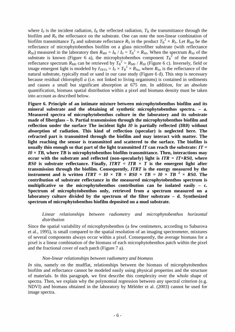
Figure 7. Spectral model of area mixtures with one microphytobenthos component andcomparison of reflectance dependence on biomass – a. Principle of a macroscopicmixture within an area S: two kinds of surface cover, area S1 and area S2 respectively,with S = S1 + S2. Reflectance of the surface S is a linear combination of reflectance ofeach material (R1 and R2) with their fractional cover: R = (S1 / S) × R1+ (S2 / S) × R2 –b. Difference between a macroscopic mixture modeled by a linear combination ofspectra and spectral variations due to natural biomass: this is evidence of a non-linearrelationship between reflectance and biomass – c. Non-linearity effects onmicrophytobenthos spectra depend on the wavelength.

A possible explanation for this non-linearity is that the biofilm thickness increases withbiomass; the thicker the biofilm, the longer the optical path. The Beer-Lambert law (2)provides a relationship between reflected light and the optical path length through atransparent material:

( )dII α−= exp0 , (2)

where I and I0 are the emergent and incident radiations respectively, α is an absorptioncoefficient and d is thickness. However, modeled spectra derived using thickness as a singleparameter are inaccurate (Figure 8 b). In the case of microphytobenthos biofilm, increasingbiomass may be due to a higher bulk density rather than an increase in the biofilm thickness.This discrepancy with respect to the theory may be explained partially by light scatteringbetween microphytobenthos cells and also by particulates of the sediment. Particles of sizeranging roughly from less than 1 µm up to 200 µm and material porosity are able to scatterradiations in the visible-infrared domain. This can significantly change reflectance level andthe slope of spectra and can also affect relative absorption band depths. Such an effect canonly be taken into account by comparing the spectra to a library simulation of a large varietyof cases (section 2.3).

In the laboratory, all these structural variations are less important than on the mudflat, sobiomass can be predicted from a spectral criterion like NDVI or any other index (Méléder etal., 2003). On field spectra, this kind of relationship is able to provide relative quantification.For an absolute quantification in situ, biomass should be measured on samples from themudflat. Moreover, the situation is complicated on image spectra.

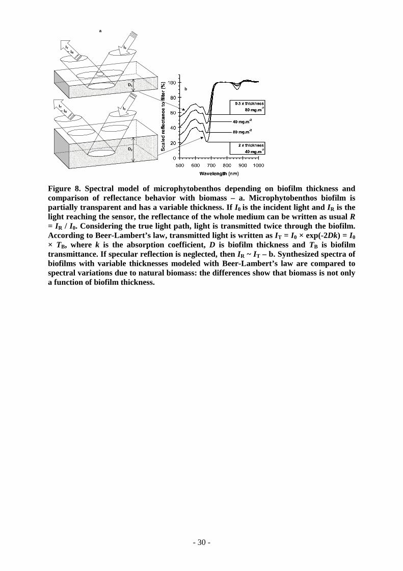
Figure 8. Spectral model of microphytobenthos depending on biofilm thickness andcomparison of reflectance behavior with biomass – a. Microphytobenthos biofilm ispartially transparent and has a variable thickness. If I0 is the incident light and IR is thelight reaching the sensor, the reflectance of the whole medium can be written as usual R= IR / I0. Considering the true light path, light is transmitted twice through the biofilm.According to Beer-Lambert’s law, transmitted light is written as IT = I0 × exp(-2Dk) =

- 8 -

I0 × TB, where k is the absorption coefficient, D is biofilm thickness and TB is biofilmtransmittance. If specular reflection is neglected, then IR ~ IT – b. Synthesized spectra ofbiofilms with variable thicknesses modeled with Beer-Lambert’s law are compared tospectral variations due to natural biomass: the differences show that biomass is not onlya function of biofilm thickness.

Scaling effects

The distance to the target is another key parameter. Scaling effects between fieldmeasurements and remote sensing data are thought to introduce strong deviations (Friedl etal., 1995; Chen, 1999). This is particularly true when an interface between contrastedmaterials occurs within a pixel (Chen, 1999). An empirical solution is to remove thecontinuum as described in section 2.2.

Considering the direct problem

We have found correlations between biomass and radiometry only when all other parameters(fractional cover, substrate, mixture with other materials) are kept constant. Consequently, thenumber of parameters varying together causes a strong non-linearity. The lack of a simplerelationship does not allow the inversion of reflectance spectra to determine biomass: a moreappropriate method is needed. To answer the challenge of an absolute biomass quantification,we have considered the direct problem. The method presented in this paper is based on thecomparison of image and field spectra with a spectral library of mixtures using spectraldistance.

3. Modeling of measured spectra

3.1. Inversion of the spectraTo extract the maximum information from the substrate, the continuum shape should be basedon both physical knowledge and measured reflectances. The Modified Gaussian Model(MGM) developed by Sunshine et al. (1990) allows such decomposition. The MGM sourcecode is available on-line (Sunshine et al., 1998) in IDL (Interactive Data Language) andFortran.The spectral deconvolution by MGM uses a non-linear least-squares analysis. As described inEquation 3, the measured spectrum reflectance R at a given wavelength λk is fitted by asuperposition of n Gaussian distributions (each is defined by three parameters: centralwavelength µ, half-width σ and negative strength s) and a continuum curve (slope a andintercept b for a straight line in wavenumber).

( ) ( ) ( )∑

=

−

−−⋅++=n

i i

ikikk sbaR

12

2

1

2expln

σµλλ . (3)

Classical Gaussian models assume each absorption band is randomly distributed in energyand thus in the wavenumber space. Because MGM was designed for mineral analysis, itassumes Gaussian curves in wavelength (the modified shape) instead of Gaussian curves inenergy (or wavenumber). In the present paper, we also used the MGM source code forspectral decomposition and data reduction capabilities.The solution is obtained by a least-square fit of the actual spectrum and is modeled by solvingthe 3n+2 normal equations, involving the partial derivatives relative to the 3n+2 parameters,which are also the unknowns. Since the synthesized spectrum function is non-linear, the set ofnormal equations is solved iteratively using first order Taylor expansion of Equation 2. The

- 9 -

iterative process, described in Tarantola and Valette (1982), converges to a solution that isaccepted if the residual becomes lower than a defined threshold. The inversion includes aprocess that prevents the strength from becoming positive (Hiroi et al., 2000). If noconvergence is found, the iterative process is stopped.Although the MGM was originally designed for individual spectra, we upgraded it to handlelarge data sets. The inversion process must start with an initial set of parameters that is chosenby observing the spectral shapes and an a priori knowledge about spectra and the continuum(Table 1 a).Concerning absorption features, an initial set of parameters is determined from the a prioriknowledge we have of the surface composition. For microphytobenthos, we used band centersdetermined by laboratory experiments (Méléder et al., 2003). With DAIS spectral resolution,all pigment absorptions cannot be resolved, leading to a non-negligible shift of the MGMcenters. To avoid important fluctuations from experimental measurements, all centers µ arelocked: 2n+2 free parameters remain. Despite these constraints, a good fit is obtained with aminimum number of functions. Bandwidth values are also needed before any iteration buttheir precision does not influence significantly the solution.MGM starts with an initial set of parameters (Table 1 a) that includes absorption band centersand Full-Width at Half-Maximum (FWHM). For each spectrum, a continuum slope isdeduced from reflectance values. Then, each absorption strength is estimated by calculatingthe difference between the continuum and the spectrum. Final Gaussian band strengths,widths and centers plus the continuum slope and intercept constitute the results (Table 1 b).MGM provides parameters on each individual absorption band. These are reliable under theconditions of linear mixture and without saturation. In microphytobenthos spectra, saturationmay distort the 675 nm absorption band at high chlorophyll a concentrations (Méléder et al.,2003) but, in the area we have studied, saturation is never encountered. Intimate mixtures arethe general rule (as mentioned above) and DAIS spectral resolution is not good enough todistinguish individual phytopigment absorptions. Consequently, Gaussian parameters for eachphytopigment absorption are not used directly for an absolute quantification. However, otherlarge features like water absorption at 980 nm and continuum can be exploited.

Table 1. Microphytobenthos absorption band centers and Full-Width Half-Maximum(FWHM) used for MGM parameters associated with photosynthetic and accessorypigments (Méléder et al., 2003), cell structure and water – a. This initial set of Gaussianparameters is valid for all the pixels before computation. The center at 435 nm is outsidethe lower limit of the wavelength range but the red wing of the associated absorption isdetectable by DAIS and can also be fitted. The parameters for the continuum andstrengths are not represented because their estimation varies from one pixel to another –b. Example of final parameters for one pixel. Centers are fixed at their initial value.

3.2. ContinuumFor the continuum, we choose a straight-line function in wavenumber (Sunshine et al., 1990,1993, 1998). The initial intercept and slope are based on the infrared straight line in the range800-900 nm, which is pertinent to the present study because it is free of phytopigmentabsorptions. The continuum is representative of the characteristics of the substrate (Méléder,2003) such as grain size. More generally, no mineral absorption band is predominant atwavelengths lower than 900 nm, so the differences between airborne and groundmeasurements in the smooth reflectance portion might be sensitive essentially to observationconditions, through and above the atmosphere respectively. The substrate varies from onepixel to another and each spectrum has its own continuum.For each pixel, MGM also provides a synthetic spectrum and a spectrum standardized to the

- 10 -

continuum. Graphs in Figure 9 show the main characteristics of a continuum fitted globally.One of the most important results is that the shape and the slope of the final continuum do notperfectly match the spectrum at 500 nm: low reflectances at short wavelengths are explainedby several absorption bands rather than a low continuum. On the other hand, the continuum isslightly above the measured spectrum between 800 and 900 nm. This position is a result ofMGM that shifts the continuum at shorter wavelengths to fit the overall spectrum by Gaussiancurves. This behavior indicates the relevance of the continuum provided by MGM because allabsorptions are explained Gaussian curves thus the continuum varies independently of theseabsorptions.

Figure 9. Example of one DAIS spectrum of microphytobenthos fitted by MGM byseveral Gaussian curves and a continuum represented in different spaces. Note that onthe three figures, the spectrum modeled by MGM is slightly shifted below the spectrumsince the two curves could not be distinguished otherwise. – a. Natural logarithmreflectance versus wavenumber. In this space, the spectrum is fitted by the MGM – b.Natural logarithm reflectance versus wavelength: one can see the shape of thecontinuum – c. Reflectance versus wavelength. Vertical dashed lines point out allpigments and water absorption centers (see Table 1).

Because of the complex relationship between the shape of spectra and biomass, asdemonstrated above, some of these differences are contained in the continuum. Thus, theMGM-derived continuum is removed from both the DAIS and the library spectra. Theremaining absorption bands are assumed to be more representative signatures forquantification. Figure 10 shows a comparison of continuum fitted by MGM on endmemberspectra from DAIS data (Figure 10 a). Spectra after standardization by MGM continuum aredisplayed in Figure 10 b.

Figure 10. DAIS spectra of characteristic surface types of Bourgneuf Bay – a. with theirrespective continuum – b. after continuum removal.

Comparison of DAIS and GER spectra of microphytobenthos shows a rather good match afterreflectance standardization by MGM continuum (Figure 11). Chlorophyll a and chlorophyll cfeatures do not appear as separated absorption bands but quantification is still possible.However, small differences are found systematically in the shape of the chlorophyll aabsorption band at 675 nm. A better match is obtained when GER 3700 resampling to DAISis done by degrading the spectral resolution by 25% with respect to DAIS specification.

Figure 11. –Spectral resampling (after continuum removal) from GER 3700 (darksmooth curve) to DAIS: the laboratory microphytobenthos spectrum (triangles) matchesthe DAIS spectrum (circles) in the range 500-800 nm used for biomass quantification.Absorption around 980 nm is due to water. The DAIS original sampling (crosses) hasbeen slightly modified (triangles) to preserve the slope in the chlorophyll a absorptionband at 675 nm.

3.3. Building a reference libraryThis step provides a spectral database in which each spectrum will represent a mixture of allspectral endmembers within a pixel. This reference library will then be used to find the bestmatch with airborne spectra (cf. section 2.4). Indeed, airborne-measured spectra resultnecessarily in a macroscopic mixture of all spectral components, due to a spatial resolutionoften coarser than natural spatial variations. For microphytobenthos, as described by Saburova(1995) and Méléder (2003), possible patch sizes are in the range of square centimeters tosquare meters. So the spectral library has to be as complete as possible to include spatial

- 11 -

distribution with a special focus on the patchiness of microphytobenthos. The probability of acloser match by minimum distance between image and ground measurements should beimproved by increasing the number of reference spectra. We built synthetic reference spectrato simulate mixtures, assuming linear combinations of homogeneous areas of various knownconcentrations of microphytobenthos.Assuming that similar spectral signatures are due to the same endmember combination,airborne-measured reflectances are then compared to the library. Close spectra are assumed tocorrespond to almost identical biomasses. Because of the non-linearity introduced by theintimate mixture between biofilm and substrate, building mixtures directly and thencomparing them with measurements provides easier and better estimates than resolving theinverse problem of unmixing.The more spectral endmembers within a pixel, the larger the number of solutions of thespectrum built by varying a number of parameters becomes. These parameters aremicrophytobenthos biomass (15 samples), microphytobenthos spatial distribution (10Gaussian profiles), fractional cover for each endmember (10 % precision within a pixel),endmembers for macroscale mixtures (macroalgae, mud, sand and microphytobenthos) andendmembers for microscale or intimate mixtures (mud, sand).Ten profiles of linear mixtures for fifteen biomasses provide 150 synthesized spectra ofmicrophytobenthos biofilm only. Linear mixtures of the four main classes of spectra(macroalgae, mud, sand and microphytobenthos) with 10 % in precision within a pixel resultin 286 mixtures. For a given substrate, the number of modeled spectra is 150 × 286 = 42900.Finally, with two substrates, 2 × 42900 = 85800 spectra are computed.

Choice of endmembers

We have considered two levels of endmembers. In Bourgneuf Bay, the most representativeare contained in four groups: mud, wet sand, macroalgae and microphytobenthos. Because theobjective is to quantify microphytobenthos, and because biomass variations are difficult topredict from any spectral criterion, a second level of endmembers is composed of severalmicrophytobenthos biomasses. Biomasses are selected to be representative of naturalvariability to enable efficient processing. Very high concentrations (>200 mg.m-2) can occurin Bourgneuf Bay on a very small scale (a few cm2 according to Méléder, 2003). After severaltrials on pixels occurring on the relative highest biomass in microphytobenthos, it appears thatspectra corresponding to models including biomass higher than 100 mg.m-2 never find anymatch. Consequently, selected biomasses range from 1 mg.m-2 to 105 mg.m-2.

Sub-pixel fractional cover estimation

Any component may be present with a complex spatial distribution within a pixel thus it isnecessary to build spectra corresponding to different fractional covers. Mixture spectra areobtained by linear combination of fractional covers with endmember spectra. Since there aretwo kinds of endmember, mixtures are computed in two steps.For the group containing the four classes, we have chosen fractional covers ranging from 0 to100 %, by steps of 10 %. For a sub-pixel quantification, 10 % of the pixel area (the bestprecision expected for deconvolving any mixture) is considered as a reasonable value. Alarger part would be of no interest for mixture modeling. Conversely, a more precise modelwould require smaller uncertainties in the signal: although differences due to calibration arebetter than 5% (Figure 4), there are other sources of noise (e.g. instrumental deviation andscaling effects).According to Saburova et al. (1995), microphytobenthos biomass is not homogeneous withina pixel. Thus, we have also computed mixtures. However, patches of various densities areorganized in groups at different scales. As we were not able to predict the exact curve

- 12 -

function, the spatial distribution of microphytobenthos is modeled by Gaussian distributionscentered on biomass values measured in the laboratory (Méléder et al., 2003). For eachcentered biomass, ten profiles with variable widths (Figure 13) were calculated. Modelingspatial distribution in homogeneous patches of microphytobenthos biofilm is built by linearmixing of the fifteen biomasses. This model is assumed to take into account the biomassrange, the spatial distribution of concentrations within a pixel or a general distribution pattern.

Figure 13. Model of linear mixtures of microphytobenthos biomasses to take account ofbiofilm patchiness. Example of random spatial distributions of microphytobenthosbiomasses for an average of 68 mg.m-2 (Gaussian curves). For each of the 15 biomasses(highlighted with vertical dashed lines) measured in the laboratory by Méléder et al.(2003), 10 mixtures have been calculated with the assumption of a Gaussian distribution.

Background substitution and microscale mixture variability

The background of the resulting spectral library is however quite different from the mudflatspectra. It is removed by dividing each spectrum of the library by the spectrum of thefiberglass filter.Since we have to simulate a realistic spectral library of microphytobenthos biofilm lying ontop of various sediments of Bourgneuf Bay, each spectrum of the library is then multiplied bya background of mud or sand. In the field, that background is made of mineral componentsand organic pigments intimately mixed in the sediment. Not taking other organic pigmentsinto account would lead to a systematic biomass overestimation of the microphytobenthosbiofilm. This drawback is avoided by multiplying the spectral library by field spectra ofsubstrates containing residual amounts of chlorophyll like those of Figure 12.Despite their variable brightness, only one spectrum of bright mud (common at the top ofmost mudflats) and one spectrum of wet sand (also common towards the shoreline) are usedto build the spectral library. It has been found that including other substrates does not improvethe spectral diversity.

Figure 12. Different kinds of substratum found in Bourgneuf Bay: dark and brightmuds and sand.

Biomass look-up table

The final look-up table attached to the library includes not only biomasses but also spatialdistributions of microphytobenthos fractional cover of the fifteen reference biomasses. Agood match between image spectrum and synthetic spectrum gives direct access, through thelook-up table, to fractional cover and concentration. As spectral mixtures of the library arebuilt numerically, the exact proportion of each microphytobenthos endmember is known sothe corresponding total biomass is given by Equation 4:

( ) ( )∑=

⋅=15

1i

ibixBiomass (4),

where i is the index of the microphytobenthos endmember, x is the fractional cover and b thebiomass. By spectral comparison, each pixel of the image will be linked to one mixture of thelibrary. When a spectrum of the library is paired with the spectrum of a pixel, that pixel canbe displayed with various look-up tables showing either each component of the mixture or thetotal coverage and the total biomass.

- 13 -

3.4. Biomass quantification from the image

Spectral range of comparison

For an accurate evaluation of the biomass, spectra have to be compared to the library in thespectral range where microphytobenthos pigments dominate reflectance, namely between 496and 727 nm (14 channels). At longer wavelengths, spectra may be sensitive to the presence ofwater at the top of the mud (Figure 14). A thin layer of clear water adds absorption features at950 nm, which induce a negative slope towards shorter wavelengths and change thecontinuum estimation by MGM in the 800-900 nm range. Laboratory experiments by Méléderet al. (2003) give accurate biomass quantification through a water layer up to 5 cm. Beyondthis limit, detection of microphytobenthos is still possible but without absolute quantification.Consequently, on the image, a selection of channels is used as a mask to eliminate deep-waterareas.

Figure 14. Relative water layer thickness at the surface of the mudflat derived from the980 nm absorption band. Depth of this absorption is estimated by MGM – a. Spatialdistribution of water: map derived from the depth of the water absorption bandmeasured by a Gaussian curve from MGM – b. Spectral absorption in the near infrareddomain on microphytobenthos areas covered by a water layer of variable thickness. Ashallow layer (profile 1) mainly affects the 800-1000 nm range: microphytobenthos isstill detectable. Laboratory experiments by Méléder et al. (2003) showed that absolutebiomass quantification is possible through 5 cm of clear water. With a deeper layer(profile 2), spectra lose their microphytobenthos signature. Locally, thickness can reach1 meter.

Spectral distance comparisonA common method of spectral comparison is to consider spectra as vectors, to whichEuclidean geometry can be applied. Two spectra can then be compared based either on angleor on distance (Bakker et al., 2002). The angular separation (McMurty et al., 1974) betweentwo spectra w and v (or two vectors w and v noted conventionally either with bold charactersor with normal characters surmounted by an arrow), later defined as a spectral angle (SA) byKruse et al. (1993), can be calculated with a normalized vector product:

Figure 15. Description of metrics that can be used for comparison between spectra from alibrary and image spectra. Spectral Angle (SA) (Kruse et al., 1993) and Intensity Distance(ID) are commonly used – a. Definition of SA and ID with two-band spectra (v and w)represented as vectors in a 2-D space (Bakker, 2002). With many channels, SA and ID arecalculated in the same way – b. Consequences of SA and ID calculations. Given a set ofairborne spectra (vA, vB) and a set of reference spectra (wA, wB), pairs of vectors (vA, wA),(vB, wB), (vA, wB) and (vB, wA) define the same angle α: SA is insensitive to the mean valueof spectra. On the other hand, ID (vA, wA) < ID (vB, wB) and ID (vB, wA) < ID (vA, wB):the mean value of the spectra is preserved when using distance. ID is more sensitive to thedifference between high level spectra (bright surface) (circle centered on B) than between lowlevel spectra (dark surface) (A). In order to have equivalent distances, one must normalizewith respect to a reference spectrum.

⋅

⋅=−

wv

wvwvSA

1

cos),( . (5)

The spectral angle is independent of the length of the two vectors. In Figure 15 b, spectrafrom dark and bright materials are indexed respectively with subscript a (va, wa) and b (vb,wb). If only spectral angle is used, intensity information is lost.

- 14 -

=

bb

bawvSAwvSA ,, . (6)

This property is interesting to remove albedo variations and topographic effects (e.g. Launeauet al., 2002). In the present study, elevation is constant and the continuum is removed(standardized reflectances, section 1.3). Since albedo variations contain information that isneeded for quantifying the amount of any component present within a pixel, intensity distanceis more pertinent than spectral angle.According to Beer-Lambert’s law, absorption varies exponentially with optical depth (d).Therefore, it seems more appropriate to use the natural logarithm of standardized reflectance.The difference between two vectors v and w becomes the ratio of their respective reflectance.The intensity distance (ID) is calculated as the absolute difference in length of v and w:

wvwvID −=),( . (7)

Because of the exponential dependence of absorption intensity I on the absorption coefficientα and optical depth d (Eq. 2: Beer-Lambert law), the intensity distance has a more physicalsignificance if calculated with natural logarithm reflectances.

With classical percent reflectances ρ, an equivalent formulation of ID is to consider the ratiobetween v and w. The intensity distance (Eq. 7) is still very sensitive to the referencespectrum. This is a key point to determine which spectrum from the library is closest to thatfrom the image. That is why the spectrum to be matched (from the image) is considered as areference, while the matching spectrum to be found (from the library) is the unknown. Wesearch for the library spectrum that minimizes ID. When the brightness of a reference vectorwa increases, it becomes wb: spectral distance SD can reach larger values and the distanceequivalence is lost. Consequently, comparison of an unknown vector v to a reference vector wis more relevant if the intensity distance is divided by the length of the reference vector (Eq.8):

( )( ) ( )( )( )( ) w

wv

nwvSD

w

wv

−=

−= ∑λ λρ

λρλρ2

ln

lnln1),( . (8).

Launeau et al. (2002) used such a distance SD with normalized reflectances to map mineralcomponents. In this study, Eq. 8 was applied with reflectance after continuum removal. Thecalculation of Eq. 8 is more discriminating than the spectral angle: va and vb have the samevalue of α (Eq. 6 and Figure 15 b) while a difference appears in Eq. 9:

>

bb

ba wvSDwvSD ,, . (9)

4. Application to DAIS images

4.1. Endmember mappingComparing the distance between the image and the library provides a classification: eachpixel matches one synthetic spectrum of the library. For this spectrum, sub-pixel proportionsare known for all the endmembers, namely each mineral substrate, macroalgae and eachmicrophytobenthos biomass. To improve the clarity of the map, all the terrestrial areas havebeen masked.

The macroalgae map (Figure 16) is important to check the discrimination withmicrophytobenthos. As it is also a vegetation endmember, confusion is possible due tocommon pigments. This fractional cover map gives a spatial distribution that can be compared

- 15 -

to other endmembers and especially the various microphytobenthos biomasses. Macroalgaeare present at specific locations, mainly outcropping rocks. The maximum fractional cover isalways found at the center of these areas and partial cover, less than 40 %, is found wheremixtures with sediments or biofilms occur.

Figure 16. Map of macroalgae (dominated by the genus Fucus) and terrestrialvegetation (Spartina grass) in Bourgneuf Bay. A white mask delimits the intertidal zone.Most of the remaining area is free of upper vegetation; this occurs on outcropping rocksand is mainly concentrated on the southeastern part of the image (zoom). This selectedzone has been studied in detail because of intense mixtures between microphytobenthosand macroalgae.

Among the various microphytobenthos biomasses retained as references (fifteen valuesbetween 0.5 and 105.8 mg.m-2), Figure 17 shows a selection of spatial distributions for threeendmembers extracted from the synthetic mixtures of the library attached to each pixel.Looking at the whole image, low biomasses cover a larger part of the intertidal zone than highbiomasses (Figure 17 b). However, at some locations, the highest fractional cover is found forintermediate biomass. This indicates that a detailed analysis of the biomass spatial distributionis possible. Final results given by total quantification are displayed in Figure 18.

Figure 17. Examples of maps of microphytobenthos sub-pixel fractional cover derivedfor three biomasses of the library – a. 2 mg.m-2 – b. 14 mg.m-2 – c. 35 mg.m-2.

4.2. Biomass quantificationThe aim is to quantify the total microphytobenthos biomass per pixel (Equation 4),independently of spatial heterogeneity and variable biomass of each microphytobenthos patch.Moreover, the main structure of each endmember (Figure 17) is compared with those of totalbiomass (Figure 18 a) and total fractional cover by microphytobenthos (Figure 18 b) toanalyze the significance of its distribution over the whole intertidal zone. The higher sub-pixelfractional cover is found for low biomass biofilm that is most common on the mudflat. Highbiomass sub-pixels usually appear in smaller areas at the center of low biomass areas wherethe biofilm can reach a higher biomass. Plausible values of biomass and spatial coherence arealso obtained when high variations of phase angle occur, for example on ridges and runnels(Arrow 1, Figure 18). The presence of chlorophyll a is detected in turbid water (Arrow 2,Figure 18) at the lower limit of the intertidal zone but without reliable quantification becauseof the continuum slope change.

Figure 18. Microphytobenthos quantification by minimum distance in the visiblespectral domain (14 channels: 496-727 nm) – a. Total biomass – b. Total fractionalcover. Arrow 1: ridges and runnels. Arrow 2: resuspended microphytobenthos in thewater. Ellipse 3: small patches of high-density biofilm inside a pixel with oyster beds.Ellipse 4: low biomass with high fractional cover by microphytobenthos.

The total fractional cover (Figure 18 b) generally increases with biomass (Figure 18 a). Someareas of low fractional cover display noisy distributions of high biomasses (Arrow 3, Figure18) because microphytobenthos is covered with macroalgae and oyster beds (compare withFigure 19). In effect, this method cannot detect the presence of microphytobenthos underneathany mask. However, if this mask does not entirely cover a surface, like oyster beds ormacroalgae, microphytobenthos can be detected through the interstices.Low biomasses, about 5 mg.m-2, can also be encountered in high fractional cover of sandyareas (Arrow 4, Figure 18). This can be attributed to the presence of differentmicrophytobenthic species, living on a sandy substratum that does not form biofilm, namelyepipsammic species (Méléder, 2003). In our spectral library, sand is considered as a possible

- 16 -

substrate but laboratory reflectance measurements have been performed on species specific toa muddy environment: epipelic species (depending on availability). However, speciesdiscrimination is possible with the GER 3700 spectrometer based on their specific set ofpigments. This is not possible for DAIS spectral resolution.

4.3. Discussion and perspectivesIn Bourgneuf Bay, the understanding of the spatial distribution of microphytobenthos versusmacroalgae has been improved with respect to previous maps based on multispectral data.SPOT images were successfully used by Méléder et al. (2003) to qualitatively mapmicrophytobenthos spatial distribution and its variations with time. However, deriving anabsolute biomass and discriminating between microphytobenthos and macroalgae wasimpossible with only three bands available.In addition, spectral analysis techniques using the full spectral resolution of hyperspectral datagive more accurate results than classical methods like indices. As an example, the closecoexistence of micro- and macroalgae occurs mainly in the southeastern region (Figure 16 b),and is a frequent source of problems for microphytobenthos identification (Méléder et al.,2003 b) and other biomass quantification. With the present method, macroalgae (Figure 16)are well identified: they cover only a small portion of the image and are confined to rockylocations and a few oyster beds as can be seen in the south of Bourgneuf Bay (Figure 19).

Figure 19. Identification and quantification of microphytobenthos on a complex area(benthic diatoms on mudflats, macroalgae on rocks and Spartina grass). Comparison ofdifferent techniques – a. NDVI – b. Specific index for microphytobenthos used byMéléder, 2003 – c. Microphytobenthos biomass from NDVI calibration by Méléder,2003. – d. Microphytobenthos biomass from a comparison of spectral distance with alibrary of synthetic mixtures (present method).

Since microphytobenthos contains chlorophyll, its reflectance (R) presents the standard rededge of vegetation. Méléder (2003) tested a hyperspectral NDVI (R798 nm-R675 nm)/(R798 nm+R675

nm) with DAIS data as a quantification tool (Figure 19 a). This has a higher sensitivity tomacroalgae than to microphytobenthos biofilm, leading to confusion with macroalgae. Amore selective index is obtained by 2×R586 nm/(R496 nm+R675 nm) because reflectance R at 586nm is a local maximum in microphytobenthos reflectance between diadinoxanthin andchlorophyll a absorptions, at 496 nm and 675 nm respectively. This index increases withconcentration in microphytobenthos and is not sensitive to the presence of macroalgae (Figure19 b). However, it is more sensitive to saturation effects and it decreases when the highestbiomasses are encountered, leading to an underestimation (see Méléder et al. 2003 b). Thisindex is however useful to mask the macroalgae on the NDVI map (see 1 in Figure 19 c).Since the NDVI is proportional to the microphytobenthos biomass, a look-up table,established by Méléder et al. (2003 b), could be used to convert the NDVI into biomass(Figure 19c).As a validation, the results of the spectral matching technique (Figure 19 d) are compared toNDVI. Agreement must be found where the presence of microphytobenthos is not ambiguous,namely for high biofilm densities (>25 mg.m-2). Effectively, at large scale, maximumdensities occur at the same locations and have similar values. Improvements are expectedeverywhere the mask has been applied and also at the borders of the mask, near macroalgae.Distributions are quite different where biomasses are below 25 mg.m-2: the present method ismuch more sensitive to low concentrations of microphytobenthos, which is consistent withexpectations. In most places (two in Figure 19c and d), microphytobenthos presents biomassvalues around 20 mg.m-2 higher than in the calibrated NDVI map that gives 4 mg.m-2. This

- 17 -

means that significant biomass values were missed by NDVI + mask but are now detectableusing hyperspectral data with appropriate techniques.

5. ConclusionClassical remote sensing revealed the possibility of detecting and quantifying concentrationson pure surface types. Simple processing methods, like three color composites and bandratios, or more elaborate ones, like Minimum Noise Fraction Transform or Linear Unmixing,are sufficient to obtain valuable results. Nevertheless, they all suffer from a lack ofdiscrimination of multiple mixture compositions, especially when these occur at microscalewith non-linear intimate mixing or when different components present similar spectra.Consequently, resulting concentrations are wrongly estimated. A new approach was needed toavoid such confusion between different types of material inside the same family. At the sametime, sensitivity had to be improved to detect very low levels of biomass.The main principle of the procedure presented here is to solve the direct problem bycomparing a synthesized spectral library with airborne spectra. In order to compare the shapeof spectral features produced by biomass, other contributions have to be removed fromreflectance data sets. One of them is contained in a continuum that is assumed to be linear inwavenumber and estimated by the Modified Gaussian Model. A comparison is made by usingspectral distance metrics. The results give concentration maps and sub-pixel relative fractionalcover of all spectral endmembers and are in good agreement with field observations. The useof hyperspectral data and the procedure presented here provides improvements with respect toresults from multispectral images. The better spectral resolution is able to discriminate moresurface components through their specific signatures. Moreover, spectral analysis techniquesare well adapted to enhance this information. To complete the validation, uncertaintyestimations must be analyzed in further detail.Finally, comparison with computed libraries is a powerful tool to quantify any surfacecomposition under complex mixture conditions. The mudflats of Bourgneuf Bay offer aninteresting opportunity for spectral analysis improvements. New insights for other mineraland biological studies are now conceivable on more complex environments (irregulartopography, a larger diversity of vegetation) and all planetary surfaces observed byhyperspectral instruments with a sufficient number of channels. It is not realistic to choose asmall set of channels to map any material made of complex mixtures, and multispectral dataare clearly under-dimensioned. The development of remote quantification techniques, aspresented in this work, is directly linked to the development of airborne and satellite highspectral resolution mapping spectrometers.

- 18 -

AcknowledgementsWe thank Andreas Müller, HySens project manager at DLR. This airborne campaign wassupported by the European Community (Access to Research Infrastructures action of theImproving Human Potential Program). We also thank the DLR teams for image calibrationquality (German Aerospace Center and German Remote Sensing Data Center) and especiallythose involved in the Hysens program: Stephanie Holzwarth (geocoding), Rolf Richter(atmospheric correction) and Martin Habermeyer (system correction).

- 19 -

References

Adams, J.B., Smith, M.O., Gillespie, A.R. (1993). Imaging spectroscopy: interpretation basedon spectral mixture analysis. In C.M. Pieters & P.A.J. Englert (Eds.). Remote GeochemicalAnalyses: elemental and mineralogical composition, vol. 7 (pp. 145-166). Cambridge, UK:Cambridge University Press

Bakker, W.H., Schmidt, K.S. (2002). Hyperspectral edge filtering for measuring homogeneityof surface cover types. ISPRS Journal of Photogrammetry & Remote Sensing, 56, 246-256

Börner, A., Wiest, L., Keller, P., Reulke, R., Richter, R., Schaepman, M., Schläpfer, D.(2001). SENSOR: a tool for the simulation of hyperspectral remote sensing systems. ISPRSJournal of Photogrammetry & Remote Sensing, vol. 55, issue 5-6, 299-312

Carrère, V., (2003). Mapping microphytobenthos in the intertidal zone of Northern Franceusing high spectral resolution field and airborne data. 3rd EARSeL Workshop on ImagingSpectroscopy, Herrsching, Germany

Carrère, V, Spilmont, N, Davoult, D. (2004). Comparison of simple techniques for estimatingchlorophyll a concentration in the intertidal zone, using high spectral resolution fieldspectrometer data. Marine Ecology Progress Series, in press.

Chandrasekhar, S. (1960). Radiative transfer. Dover, New-York

Chen, J.M., (1999). Spatial scaling of a remotely sensed surface parameter by contexture,Remote Sensing of Environment, 69, 30-42

Clark, R.N. and Roush, T.L. (1984). Reflectance Spectroscopy: quantitative analysistechniques for remote sensing applications. Journal of Geophysical Research, vol. 89, no. B7,6329-6340

Clark, R.N. Swayze, G.A., Livo, K.E., Kokaly, R.F., Sutley, S.J., Dalton, J.B., McDougal,R.R., Gent, C.A. (2003). Imaging spectroscopy: Earth and planetary remote sensing with theUSGS Tetracorder and expert systems. Journal of Geophysical Research, vol. 108, no. E12,5131

Cognie, B., Barillé, L. and Rincé, Y. (2001). Selective feeding of the oyster Crassostrea gigasfed on natural phytobenthos assemblage, Estuaries, 24 (2), 126-131

de Jong, S. (1998). Imaging spectrometer for monitoring tree damage caused by volcanicactivity in the Long Valley caldera, California. ITC Journal, vol. 1, 1-10.

Dennison, Ph.E. and Roberts, D.A. (2003). Endmember selection for multiple endmemberspectral mixture analysis using endmember average RMSE. Remote Sensing of Environment,vol. 87, issues 2-3, 123-135

Erard, S. (2001). A spectro-photometric model of Mars in the near infrared. GeophysicalResearch Letters, vol. 28, no. 7, 1291-1294

Gross, H.N. and Schott, J.R. (1998). Application of spectral mixture analysis and imagefusion techniques for image sharpening, Remote Sensing of Environment, 63, 85-94

Friedl, M.A., Davis, F.W., Michaelsen, J., (1995). Scaling and uncertainty in the relationshipbetween the NDVI and land surface biophysical variables: an analysis using a scenesimulation model and data from FIFE, Remote Sensing of Environment, 54, 233-246

Guarini J-M. (1998). Modélisation de la dynamique du microphytobenthos des vasièresintertidales du bassin de Marennes-Oléron. Ph.D. thesis, Université de la Rochelle, 177 p

- 20 -

Hapke, B.W. (1981). Bidirectional reflectances spectroscopy 1. Theory. Journal ofGeophysical Research, vol. 86, no. B4, 3039-3054

Haure J., Sauriau, P-G., Baud, J-P. (1996). Effets du vent sur la remise en suspensionparticulaire en baie de Bourgneuf: conséquences sur la croissance de Crassostrea gigas, J.Rech. Océanographique, 11, 21-30

Herut, B., Tibor, G., Yacobi, Y.Z., Kress, N. (1999). Synoptic measurements of chlorophyll-aand suspended particulate matter in a transitional zone from polluted to clean seawaterutilizing airborne remote sensing and ground measurements, Haifa Bay (SE Mediterranean).Marine Pollution Bulletin, vol. 38, no. 9, 762-772

Kruse, F.A., Lefkof, A.B., Boardman, J.W., Heidebrecht, K.B., Shapiro, A.T., Barloon, P.J.,Goetz, A.F.H. (1993). The spectral processing system (SPIS) – interactive visualization andanalysis of imaging spectrometer data. Remote Sensing of Environment, 44, 145-163

Launeau, P., Sotin, Ch., Girardeau, J. (2002). Cartography of the Ronda peridotite (Spain) byhyperspectral remote sensing. Bulletin de la Société Géologique de France, vol. 173, no. 6,491-508

McGwire, K., Minor, Th., Fenstermaker, L. (2000). Hyperspectral Mixture Modelling forQuantifying Sparse Vegetation Cover in Arid Environments. Remote Sensing of Environment,vol. 72, issue 3, 360-374

Méléder, V., Barillé, L., Launeau, P., Carrère, V., and Rincé, Y. (2003 a). Spectrometricconstraint in analysis of benthic diatom biomass using monospecific cultures. Remote Sensingof Environment, 88, 386-400.

Méléder, V., Launeau, P., Barillé, L., and Rincé, Y. (2003 b). Cartographie des peuplementsdu microphytobenthos par télédétection spatiale visible-infrarouge dans un écosystèmeconchylicole. Comptes Rendus de l'Académie des Sciences - Biologie. 326, 377-389.

Méléder, V. (2003). Etude de la structure des peuplements intertidaux du microphytobenthos:apport de la télédétection visible infrarouge. Ph.D. Thesis

Paterson, D.M., and Hagerthey, S.E. (2001). Microphytobenthos in contrasting coastalecosystems: Biology and Dynamics. In “Ecological Comparisons of Sedimentary Shores” (K.Reise, Ed.), vol. 151 (pp. 105 – 125). Springer-Verlag, Berlin, Heidelberg

Rainey, M.P., Tyler, A.N., Gilvear, D.J., Bryant, R.G., McDonald, P. (2003). Mappingintertidal estuarine sediment grain size distributions through airborne remote sensing. RemoteSensing of Environment, 86, 480-490

Richards, J.A. and Jia, X. (1998). Remote Sensing Digital Image Analysis: An Introduction.3rd ed. Springer-Verlag Berlin, Heidelberg, New York

Roberts, D.A., Garder, M., Church, R., Ustin, S., Scheer, G., Green, R.O. (1998). MappingChaparral in the Santa Monica Mountains Using Multiple Endmember Spectral MixtureModels. Remote Sensing of Environment, 65, 267-279

Rowan, L.C., Crowley, J.K., Schmidt, R.G., Ager, C.M., Mars, J.C. (2000). Mappinghydrothermally altered rocks by analysing hyperspectral image (AVIRIS) data of forestedareas in the Southeastern United States. Journal of Geochemical Exploration, vol. 68, no. 3,145-166

Saburova, M.A., Polikarpov, I.G., Burkovsky, I.V. (1995). Spatial structure of an intertidalsandflat microphytobenthic community as related to different spatial scales. Marine EcologyProgress Series, 129, 229-239

- 21 -

Sanders, L.C., Schott, J.R., Raqueno, R. (2001). A VNIR/SWIR atmospheric correctionalgorithm for hyperspectral imagery with adjacency effect. Remote Sensing of Environment,78, 3, 252-263

Secker, J., Staenz, K., Gauthier, R.P., Budkewitsch, P. (2001). Vicarious calibration ofairborne hyperspectral sensors in operational environments. Remote Sensing of Environment,76, 81-92

Sunshine, J., Pieters, C.M., Pratt, S.F. (1990). Deconvolution of mineral absorption bands: Animproved approach. Journal of Geophysical Research, vol. 93, no. B5, 6955-6966

Sunshine, J., Pieters, C.M. (1993). Estimating Modal Abundances from the Spectra of Naturaland Laboratory Pyroxene Mixtures Using the Modified Gaussian Model. Journal ofGeophysical Research, vol. 98, no. E5, 9075-9087

Sunshine, J., Pieters, C.M., Pratt, S.F., McNaron-Brown, K.S. (1998). Absorption bandmodeling in reflectance spectra: Availability of the Modified Gaussian Model (atwww.planetary.brown.edu). Proceedings of the 29th Lunar and Planetary Space Conference.

Tarantola A and Valette B. (1982). Generalized nonlinear inverse problems solved using theleast squares criterion, Reviews of Geophysics and Space Physics, vol. 20, no. 2, 219-222.

Tompkins, S., Mustard, J.F., Pieters, C.M., Forsyth, D.W. (1997). Optimization ofendmembers for spectral mixture analysis. Remote Sensing of Environment, 59, 472-489

- 22 -

MGM resulting parameters

a

b

Table 1. Microphytobenthos absorption band centers and Full-Width Half-Maximum(FWHM) used for MGM parameters associated with photosynthetic and accessorypigments (Méléder et al., 2003), cell structure and water – a. This initial set of Gaussianparameters is valid for all the pixels before computation. The center at 435 nm is outsidethe lower limit of the wavelength range but the red wing of the associated absorption isdetectable by DAIS and can also be fitted. The parameters for the continuum andstrengths are not represented because their estimation varies from one pixel to another –b. Example of final parameters for one pixel. Centers are fixed at their initial value.

- 23 -

Figure 1. Synoptic view of the intertidal zone of Bourgneuf Bay and the location ofcomponents.

- 24 -

a b

Figure 2. Surface types of Bourgneuf Bay – a. View of the bay: a microphytobenthosbiofilm is in the foreground. A few meters farther away, outcropping rocks correspondto an ancient oyster bed and the sea is in the background. Spectra acquisition and in situbiofilm sampling is illustrated in the foreground – b. Examples of GER 3700 fieldspectra.

- 25 -

Dry sand (bright target)

Basin water (dark target)

Figure 3. Bourgneuf Bay DAIS image (RGB colors associated with channels at 496, 675and 798 nm respectively). Green: microphytobenthos; light red: terrestrial vegetation;dark blue: macroalgae; white: sand; gray: mud; blue: water.

- 26 -

Figure 4. Validation of the calibration process on a homogeneous sandy area: nosignificant difference is seen between the field GER 3700 spectrum and the airborneDAIS spectrum.

- 27 -

Figure 5. Microphytobenthos reflectance spectra of 15 monospecific diatom cultures ofincreasing concentrations deposited on a fiberglass filter substrate (Méléder et al., 2003).

- 28 -

a

I0 ITRT

(1)

(2)

b

d c

Multiplication by a spectrum of mud

Division by the filter spectrum

R2

R2

R2 = 1

Transmission path length through the

biofilm~10-200 µm

Mud

Residual Chl-a in sediments

Chl-a linked to living organisms

ITR IT

IR0

Figure 6. Principle of an intimate mixture between microphytobenthos biofilm and itsmineral substrate and the obtaining of synthetic microphytobenthos spectra. – a.Measured spectra of microphytobenthos culture in the laboratory and its substratemade of fiberglass – b. Partial transmission through the microphytobenthos biofilm andreflection under the surface The incident light I 0 is partially reflected (IR0) withoutabsorption of radiation. This kind of reflection (specular) is neglected here. Therefracted part is transmitted through the biofilm and may interact with matter. Thelight reaching the sensor is transmitted and scattered to the surface. The biofilm isusually thin enough so that part of the light transmitted IT can reach the substrate: IT =I 0 × TB, where TB is microphytobenthos biofilm transmittance. Then, interactions mayoccur with the substrate and reflected (non-specularly) light is ITR = IT×RS0, where RS0 issubstrate reflectance. Finally, ITRT = ITR × T is the emergent light after transmissionthrough the biofilm. Consequently, ITRT is the energy measured by the instrument and iswritten ITRT = I0 × TB × RS0 × TB = I 0 × TB 2 × RS0. The contribution of substratereflectance in the measured microphytobenthos spectrum is multiplicative so themicrophytobenthos contribution can be isolated easily – c. Spectrum ofmicrophytobenthos only, retrieved from a spectrum measured on a laboratory culturedivided by the spectrum of the filter substrate – d. Synthesized spectrum ofmicrophytobenthos biofilm deposited on a mud substrate.

- 29 -

S2 S1

a

Figure 7. Spectral model of area mixtures with one microphytobenthos component andcomparison of reflectance dependence on biomass – a. Principle of a macroscopicmixture within an area S: two kinds of surface cover, area S1 and area S2 respectively,with S = S1 + S2. Reflectance of the surface S is a linear combination of reflectance ofeach material (R1 and R2) with their fractional cover: R = (S1 / S) × R1+ (S2 / S) × R2 –b. Difference between a macroscopic mixture modeled by a linear combination ofspectra and spectral variations due to natural biomass: this is evidence of a non-linearrelationship between reflectance and biomass – c. Non-linearity effects onmicrophytobenthos spectra depend on the wavelength.

- 30 -

I0 IT ~ IR

I0 IT

~ IR

D1

D2

a

b

Figure 8. Spectral model of microphytobenthos depending on biofilm thickness andcomparison of reflectance behavior with biomass – a. Microphytobenthos biofilm ispartially transparent and has a variable thickness. If I 0 is the incident light and IR is thelight reaching the sensor, the reflectance of the whole medium can be written as usual R= IR / I 0. Considering the true light path, light is transmitted twice through the biofilm.According to Beer-Lambert’s law, transmitted light is written as IT = I 0 × exp(-2Dk) = I 0

× TB, where k is the absorption coefficient, D is biofilm thickness and TB is biofilmtransmittance. If specular reflection is neglected, then IR ~ IT – b. Synthesized spectra ofbiofilms with variable thicknesses modeled with Beer-Lambert’s law are compared tospectral variations due to natural biomass: the differences show that biomass is not onlya function of biofilm thickness.

- 31 -

a

b

c

Figure 9. Example of one DAIS spectrum of microphytobenthos fitted by MGM byseveral Gaussian curves and a continuum represented in different spaces. Note that onthe three figures, the spectrum modeled by MGM is slightly shifted below the spectrumsince the two curves could not be distinguished otherwise. – a. Natural logarithmreflectance versus wavenumber. In this space, the spectrum is fitted by the MGM – b.Natural logarithm reflectance versus wavelength: one can see the shape of thecontinuum – c. Reflectance versus wavelength. Vertical dashed lines point out allpigments and water absorption centers (see Table 1).

- 32 -

(Fucus sp.)

(Spartina sp.)

Figure 10. DAIS spectra of characteristic surface types of Bourgneuf Bay – a. with theirrespective continuum – b. after continuum removal.

- 33 -

Figure 11. –Spectral resampling (after continuum removal) from GER 3700 (darksmooth curve) to DAIS: the laboratory microphytobenthos spectrum (triangles) matchesthe DAIS spectrum (circles) in the range 500-800 nm used for biomass quantification.Absorption around 980 nm is due to water. The DAIS original sampling (crosses) hasbeen slightly modified (triangles) to preserve the slope in the chlorophyll a absorptionband at 675 nm.

- 34 -

Figure 12. Different kinds of substratum found in Bourgneuf Bay: dark and brightmuds and sand.

- 35 -

Figure 13. Model of linear mixtures of microphytobenthos biomasses to take account ofbiofilm patchiness. Example of random spatial distributions of microphytobenthosbiomasses for an average of 68 mg.m-2 (Gaussian curves). For each of the 15 biomasses(highlighted with vertical dashed lines) measured in the laboratory by Méléder et al.(2003), 10 mixtures have been calculated with the assumption of a Gaussian distribution.

- 36 -

Figure 14. Relative water layer thickness at the surface of the mudflat derived from the980 nm absorption band. Depth of this absorption is estimated by MGM – a. Spatialdistribution of water: map derived from the depth of the water absorption bandmeasured by a Gaussian curve from MGM – b. Spectral absorption in the near infrareddomain on microphytobenthos areas covered by a water layer of variable thickness. Ashallow layer (profile 1) mainly affects the 800-1000 nm range: microphytobenthos isstill detectable. Laboratory experiments by Méléder et al. (2003) showed that absolutebiomass quantification is possible through 5 cm of clear water. With a deeper layer(profile 2), spectra lose their microphytobenthos signature. Locally, thickness can reach1 meter.

- 37 -

Figure 15. Description of metrics that can be used for comparison between spectra froma library and image spectra. Spectral Angle (SA) (Kruse et al., 1993) and IntensityDistance (ID ) are commonly used – a. Definition of SA and ID with two-band spectra (vand w) represented as vectors in a 2-D space (Bakker, 2002). With many channels, SAand ID are calculated in the same way – b. Consequences of SA and ID calculations.Given a set of airborne spectra (vA, vB) and a set of reference spectra (wA, wB), pairs ofvectors (vA, wA), (vB, wB), (vA, wB) and (vB, wA) define the same angle α: SA is insensitiveto the mean value of spectra. On the other hand, ID (vA, wA) < ID (vB, wB) and ID (vB, wA)< ID (vA, wB): the mean value of the spectra is preserved when using distance. ID is moresensitive to the difference between high level spectra (bright surface) (circle centered onB) than between low level spectra (dark surface) (A). In order to have equivalentdistances, one must normalize with respect to a reference spectrum.

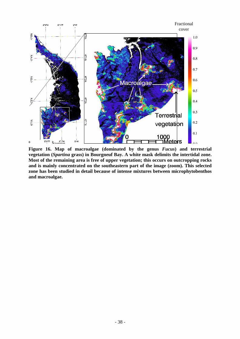
- 38 -

Fractional cover

Figure 16. Map of macroalgae (dominated by the genus Fucus) and terrestrialvegetation (Spartina grass) in Bourgneuf Bay. A white mask delimits the intertidal zone.Most of the remaining area is free of upper vegetation; this occurs on outcropping rocksand is mainly concentrated on the southeastern part of the image (zoom). This selectedzone has been studied in detail because of intense mixtures between microphytobenthosand macroalgae.

- 39 -

2 mg.m-2 14 mg.m-2 Fractional cover for

each biomass

35 mg.m-2

Figure 17. Examples of maps of microphytobenthos sub-pixel fractional cover derivedfor three biomasses of the library – a. 2 mg.m-2 – b. 14 mg.m-2 – c. 35 mg.m-2.

a b c

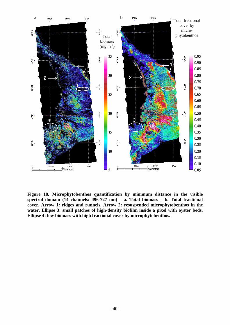
- 40 -

Total biomass (mg.m-2)

Total fractional cover by micro-

phytobenthos

a b

Figure 18. Microphytobenthos quantification by minimum distance in the visiblespectral domain (14 channels: 496-727 nm) – a. Total biomass – b. Total fractionalcover. Arrow 1: ridges and runnels. Arrow 2: resuspended microphytobenthos in thewater. Ellipse 3: small patches of high-density biofilm inside a pixel with oyster beds.Ellipse 4: low biomass with high fractional cover by microphytobenthos.

- 41 -

NDVI : (R(.798)-R(.675))/( R(.798)+R(.675))

Biomass (mg.m-2)

2xR(.586)/(R(.496)+R(.675)) a b

c d Biomass (mg.m-2)

1

1 1

1 1

1

2 2

2 2

1000 Meters 1000 Meters

1000 Meters 1000 Meters

Figure 19. Identification and quantification of microphytobenthos on a complex area(benthic diatoms on mudflats, macroalgae on rocks and Spartina grass). Comparison ofdifferent techniques – a. NDVI – b. Specific index for microphytobenthos used byMéléder, 2003 – c. Microphytobenthos biomass from NDVI calibration by Méléder,2003. – d. Microphytobenthos biomass from a comparison of spectral distance with alibrary of synthetic mixtures (present method).